Abstract

We consider a cosmological model dominated by bulk viscous matter with total bulk viscosity coefficient proportional to the velocity and acceleration of the expansion of the universe in such a way that $\zeta=\zeta_{0}+\zeta_{1}\frac{\dot{a}}{a}+\zeta_{2}\frac{\ddot{a}}{\dot{a}}.$ We show that there exist two limiting conditions in the bulk viscous coefficients, ($\zeta_{0}$, $\zeta_{1}$, $\zeta_{2}$) which corresponds to a universe having a Big-Bang at the origin, followed by an early decelerated epoch and then making a smooth transition into an accelerating epoch. We have constrained the model using the type Ia Supernovae data, evaluated the best estimated values of all the bulk viscous parameters and the Hubble parameter corresponding to the two limiting conditions. We found that even though the evolution of the cosmological parameters are in general different for the two limiting cases, they show identical behavior for the best estimated values of the parameters from both the limiting conditions. A recent acceleration would occur if $\tilde{\zeta}_{0}+\tilde{\zeta}_{1}>1$ for the first limiting conditions and if $\tilde{\zeta}_{0}+\tilde{\zeta}_{1}<1$ for the second limiting conditions. The age of the universe predicted by this model is found to be less than that predicted from the oldest galactic globular clusters. The total bulk viscosity seems to be negative in the past and becomes positive when $z\leq 0.8$. So the model violates the local second law of thermodynamics. However, the model satisfies the generalized second law of thermodynamics at the apparent horizon throughout the evolution of the universe. We also made a statefinder analysis of the model and found that it is distinguishably different from the standard $\Lambda$CDM model at present, but shows a de Sitter type behavior in the far future of the evolution.

1 Introduction

Observational data on type Ia Supernovae have shown that the current universe is accelerating and the acceleration began in the recent past of the universe [1, 2]. This was further supported by the observations on cosmic microwave background radiations (CMBR) [3] and large scale structure [4]. Despite the mounting observational evidence on this recent acceleration, its nature and fundamental origin is still an open question. Many models has been proposed to explain this current acceleration. Basically there are two approaches. The first one is to modify the right hand side of the Einstein’s equation by considering specific forms for the energy-momentum tensor $T_{\mu\nu}$ having a negative pressure, which culminate in the proposal of an exotic energy called dark energy. The simplest candidate for dark energy is the so-called cosmological constant $\Lambda,$ which is characterized by the equation of state, $\omega_{\Lambda}=-1$ and a constant energy density [5]. However, it faced with many drawbacks. Of these, the two main problems are the coincidence problem and the fine tuning problem [6]. Coincidence problem refers to the coincidence of densities of dark matter and dark energy, even though their evolutions are different, and the fine tuning problem refers to the discrepancy between the theoretical and the observational value of the vacuum constant or cosmological constant, which is assumed to drive the accelerated expansion. These discrepancies motivated the consideration of various dynamical dark energy models like quintessence [7, 8], k-essence [9] and perfect fluid models (like Chaplygin gas model) [10]. The second approach for explaining the current acceleration of the universe is to modify the left hand side of the Einstein’s equation, i.e., the geometry of the space time. The models that belong to this class (modified gravity) are the so called $f(R)$ gravity [11], $f(T)$ gravity [12], Gauss-Bonnet theory [13], Lovelock gravity [14], Horava-Lifshitz gravity [15], scalar-tensor theories [16], braneworld models [17] etc.

It was noted by several authors that the bulk viscous fluid can produce acceleration in the expansion of the universe. This was first studied in the context of inflationary phase in the early universe [18, 19]. In the context of late acceleration of the universe, the effect of bulk viscous fluid was studied in references [20, 21, 22, 23, 24]. But a shortcoming in considering the bulk viscous fluid is the problem of finding out a viable mechanism for the origin of bulk viscosity in the expanding universe. From the theoretical point of view, bulk viscosity can arise due to deviations from the local thermodynamic equilibrium [25]. In cosmology, bulk viscosity arises as an effective pressure to restore the system back to its thermal equilibrium, which was broken when the cosmological fluid expands (or contract) too fast. This bulk viscosity pressure generated, ceases as soon as the fluid reaches the thermal equilibrium [26, 27, 28].

In this paper, we analyze matter dominated cosmological model with bulk viscosity with reference to the question whether it can cause the recent acceleration of the universe. We took the bulk viscosity coefficient as proportional to both the velocity and acceleration of the expansion of the universe. The matter is basically a pressureless fluid comprising both baryonic and dark matter components. If the bulk viscous matter produce the recent acceleration of the universe then it would unify the description of both dark matter and dark energy. The advantage is that it automatically solves the coincidence problem because there is no separate dark energy component. A similar model was studied by Avelino et al. [29], but in constraining the parameters, ($\zeta_{0}$, $\zeta_{1}$, $\zeta_{2}$) using the observational data the authors fixed either $\zeta_{1}$ or $\zeta_{2}$ as zero. So it is effectively a two parameter model. In this reference the authors have ruled out the possibility of bulk viscous matter to be a candidate for dark energy. We think that one should study the model by evaluating all the parameters simultaneously, which may lead to a more mature conclusion regarding the status of bulk viscous dark matter as dark energy. In the present work we aim to such an analysis in studying the evolution of all the cosmological parameters by simultaneously evaluating all the constant parameters on which the total bulk viscous coefficient depends.

The paper is organized as follows. In section 2 we present the basic formalism of the bulk viscous matter dominated flat universe. We derive the Hubble parameter in this section. In section 3, we identify two different limiting conditions for the bulk viscous coefficients corresponding to which the universe begins with a Big-Bang, followed by an early decelerated epoch and then entering a phase of recent acceleration. We also present the evolution of the scale factor and age of the universe in this section. In section 4 we study the evolution of the cosmological parameters like deceleration parameter, the equation of state parameter, matter density and curvature scalar. Section 5 consists of the study of the status of local second law and generalized second law of thermodynamics in the model. In section 6 we presents the statefinder analysis of the model to contrast it with other standard models of dark energy. The estimation of parameters using type Ia Supernova data is given in section 7, followed by conclusions in section 8.

2 FLRW Universe dominated with bulk viscous matter

We consider a spatially flat universe described by the Friedmann-Lemaitre-Robertson-Walker (FLRW) metric,

$$ds^{2}=-dt^{2}+a(t)^{2}(dr^{2}+r^{2}d\theta^{2}+r^{2}\sin^{2}\theta d\phi^{2})$$ (1)

where $(r,\theta,\phi)$ are the co-moving coordinates, $t$ is the cosmic time and $a(t)$ is the scale factor of the universe dominated with bulk viscous matter, which can produce an effective pressure [30, 31]

$$P^{*}=P-3\zeta H$$ (2)

where $P$ is the normal pressure, which is zero for non-relativistic matter and $\zeta$ is the coefficient of bulk viscosity, which can be a function of Hubble Parameter and its derivatives in an expanding universe. We have not considered the radiation component, as it is a reasonable simplification as long as we are concerned with late time acceleration. The form of equation (2) was originally proposed by Eckart in 1940 [32]. A similar theory was also proposed by Landau and Lifshitz [33]. However, Eckart theory suffer from pathologies. One of them is that in this theory, dissipative perturbations propagate at infinite speeds [34]. Another one is that the equilibrium states in the theory are unstable [35]. In 1979, Israel and Stewart [36, 37] developed a more general theory which was causal and stable and one can obtain the Eckart theory from it in the first order limit, when the relaxation time goes to zero. So, in the limit of vanishing relaxation time, the Eckart theory is a good approximation to the Israel-Stewart theory.

Even though Eckart theory have drawbacks, it is less complicated than the Israel-Stewart theory. So it has been used widely by many authors to characterize the bulk viscous fluid. For example in references [20, 38, 39, 40], Eckart approach has been used in dealing with the accelerating universe with the bulk viscous fluid. In this context, it is reasonable to point out that Hiscock et. al.[41] have found that pathological Eckart theory and also truncated Israel- Stewart theory (avoiding the non-linear terms) can produce early inflation. However, as pointed out by the same authors, in the truncated version of Israel-Stewart theory, the relaxation time stands to be a constant which is in fact not logically correct in an expanding universe. However, there exist some later studies [42, 43] which deals with the importance of equation of state in such theories inorder to explain the acceleration. But, it should be checked whether these theories will produce the late acceleration of the universe as observed today. One should also note at this juncture that a more general formulation than Israel-Stewart model was proposed by Pavon et al. [44] for irreversible process, especially in dealing with thermodynamic equilibrium of dissipative fluid.

The Friedmann equations describing the evolution of flat universe dominated with bulk viscous matter are,

$$H^{2}=\frac{\rho_{m}}{3}$$ (3)

$$2\frac{\ddot{a}}{a}+\left(\frac{\dot{a}}{a}\right)^{2}=-P^{*}$$ (4)

where we have taken $8\pi G=1$, $\rho_{m}$ is the matter density and overdot represents the derivative with respect to cosmic time $t$. The conservation equation is

$$\dot{\rho}_{m}+3H(\rho_{m}+P^{*})=0.$$ (5)

In this paper we consider a parameterized bulk viscosity of the form [45],

$$\zeta=\zeta_{0}+\zeta_{1}\frac{\dot{a}}{a}+\zeta_{2}\frac{\ddot{a}}{\dot{a}}.$$ (6)

In an expanding universe, the bulk viscosity coefficient may depends on both the velocity and acceleration. The most logical form can be a linear combination of three terms: the first term is a constant $\zeta_{0}$, the second term is proportional to the Hubble parameter, which characterizes the dependence of the bulk viscosity on velocity, and the third is proportional to $\frac{\ddot{a}}{\dot{a}}$, characterizing the effect of acceleration on the bulk viscosity. Moreover, such a form for the bulk viscous coefficient implies the most general form of the equation of state [45]. In terms of Hubble parameter $H=\frac{\dot{a}}{a}$, this can be written as,

$$\zeta=\zeta_{0}+\zeta_{1}H+\zeta_{2}(\frac{\dot{H}}{H}+H)$$ (7)

From Friedmann equations, and from equations (2), (5) and (7), we can obtain a first order differential equation for Hubble parameter by replacing $\frac{d}{dt}$ with $\frac{d}{d\ln a}$ through $\frac{d}{dt}=H\frac{d}{d\ln a}$ as,

$$\frac{dH}{d\ln a}-\left(\frac{\tilde{\zeta}_{1}+\tilde{\zeta}_{2}-3}{2-\tilde{\zeta}_{2}}\right)H-\left(\frac{\tilde{\zeta}_{0}}{2-\tilde{\zeta}_{2}}\right)H_{0}=0$$ (8)

where

$$\tilde{\zeta}_{0}=\frac{3\zeta_{0}}{H_{0}},\ \ \ \ \tilde{\zeta}_{1}=3\zeta_{1},\ \ \ \ \tilde{\zeta}_{2}=3\zeta_{2}$$ (9)

are the dimensionless bulk viscous parameters and $H_{0}$ is the present value of the Hubble parameter. The above equation can be integrated to obtain the Hubble parameter as,

$$H(a)=H_{0}\left[a^{\frac{\tilde{\zeta}_{1}+\tilde{\zeta}_{2}-3}{2-\tilde{\zeta}_{2}}}\left(1+\frac{\tilde{\zeta}_{0}}{\tilde{\zeta}_{1}+\tilde{\zeta}_{2}-3}\right)-\frac{\tilde{\zeta}_{0}}{\tilde{\zeta}_{1}+\tilde{\zeta}_{2}-3}\right]$$ (10)

This equation shows that when $\tilde{\zeta}_{0}$, $\tilde{\zeta}_{1}$ and $\tilde{\zeta}_{2}$ are all zeros, the Hubble parameter, $H=H_{0}a^{-\frac{3}{2}}$ which corresponds to the ordinary matter dominated universe. When $\tilde{\zeta}_{1}=\tilde{\zeta}_{2}=0$, the Hubble parameter reduces to [23]

$$H(a)=H_{0}\left[a^{-\frac{3}{2}}\left(1-\frac{\tilde{\zeta}_{0}}{3}\right)+\frac{\tilde{\zeta}_{0}}{3}\right].$$ (11)

3 Behavior of scale factor and age of the universe

In this section we analyze the behavior of scale factor in a bulk viscous matter dominated universe. Using the definition of Hubble parameter, equation (10) becomes,

$$\frac{1}{a}\frac{da}{dt}=H_{0}\left[a^{\frac{\tilde{\zeta}_{12}-3}{2-\tilde{\zeta}_{2}}}\left(1+\frac{\tilde{\zeta}_{0}}{\tilde{\zeta}_{12}-3}\right)-\frac{\tilde{\zeta}_{0}}{\tilde{\zeta}_{12}-3}\right]$$ (12)

where $\tilde{\zeta}_{12}=\tilde{\zeta}_{1}+\tilde{\zeta}_{2}$. Integrating the above equation to solve for the scale factor we get,

$$a(t)=\left[(\frac{\tilde{\zeta}_{0}+\tilde{\zeta}_{12}-3}{\tilde{\zeta}_{0}})+(\frac{3-\tilde{\zeta}_{12}}{\tilde{\zeta}_{0}})e^{\frac{\tilde{\zeta}_{0}}{2-\tilde{\zeta}_{2}}H_{0}(t-t_{0})}\right]^{\frac{2-\tilde{\zeta}_{2}}{3-\tilde{\zeta}_{12}}}$$ (13)

where $t_{0}$ is the present cosmic time. Assuming, $y=H_{0}(t-t_{0})$ and taking second derivative of the scale factor $a$ (equation (13)) with respect to $y$, we obtain

$$\begin{split}\frac{d^{2}a}{dy^{2}}=&\frac{e^{\frac{\tilde{\zeta}_{0}y}{2-\tilde{\zeta}_{2}}}}{2-\tilde{\zeta}_{2}}\left[\tilde{\zeta}_{0}+\tilde{\zeta}_{12}-3+(2-\tilde{\zeta}_{2})e^{\frac{\tilde{\zeta}_{0}y}{2-\tilde{\zeta}_{2}}}\right]\\ &\left[\frac{\tilde{\zeta}_{0}+\tilde{\zeta}_{12}-3+(3-\tilde{\zeta}_{12})e^{\frac{\tilde{\zeta}_{0}y}{2-\tilde{\zeta}_{2}}}}{\tilde{\zeta}_{0}}\right]^{\frac{2(\tilde{\zeta}_{1}-2)+\tilde{\zeta}_{2}}{3-\tilde{\zeta}_{12}}}.\end{split}$$ (14)

From the behavior of the scale factor and the Hubble parameter, it is possible to identify two limiting conditions on $(\tilde{\zeta}_{0},\tilde{\zeta}_{1},\tilde{\zeta}_{2})$ which corresponds to a universe that would start with a Big-Bang followed by an early decelerated epoch, then making a transition into the accelerated epoch in the later times. These two conditions are,

$$\tilde{\zeta}_{0}>0,\,\tilde{\zeta}_{12}<3,\,\tilde{\zeta}_{2}<2$$ (15)

$$\tilde{\zeta}_{0}<0,\,\tilde{\zeta}_{12}>3,\,\tilde{\zeta}_{2}>2.$$ (16)

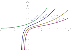
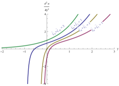
The first condition is to be simultaneously satisfied with $\tilde{\zeta}_{0}+\tilde{\zeta}_{12}<3$ and the second condition with $\tilde{\zeta}_{0}+\tilde{\zeta}_{12}>3$. Instead of these, if the first condition (15) is satisfied simultaneously with $\tilde{\zeta}_{0}+\tilde{\zeta}_{12}>3$ or the second condition (16) with $\tilde{\zeta}_{0}+\tilde{\zeta}_{12}<3$, then the universe will undergo an eternally accelerated expansion, see the curve for $\tilde{\zeta}_{0}+\tilde{\zeta}_{12}=3$ in figures 3 and 4. We have obtained the best estimates of the bulk viscous parameters $(\tilde{\zeta}_{0},\tilde{\zeta}_{1},\tilde{\zeta}_{2})$ corresponding to the cases, equations (15) and (16) separately, using the SCP “Union” SNe Ia data set, about which we will discuss in section 7.

For both the cases of bulk viscous parameters, as given by equations (15) and (16), the Hubble parameter given in equation (10) becomes infinity as the scale factor $a\to 0$, which implies that the density becomes infinity at the origin, indicating the presence of a Big-Bang at the origin. The behavior of the scale factor as given in equation (13) are shown in figures 1 and 2 for the two conditions of parameters respectively. As $(t-t_{0})\rightarrow 0$, the scale factor in both the cases reduces to

$$a(t)\to\left[1+\frac{3-\tilde{\zeta}_{12}}{2-\tilde{\zeta}_{2}}H_{0}(t-t_{0})\right]^{\frac{2-\tilde{\zeta}_{2}}{3-\tilde{\zeta}_{12}}},$$ (17)

which corresponds to an early decelerated expansion. In both the cases of limiting conditions, as $(t-t_{0})\rightarrow\infty$, the scale factor tends to,

$$a(t)\to e^{\frac{\tilde{\zeta}_{0}}{2-\tilde{\zeta}_{2}}H_{0}(t-t_{0})}.$$ (18)

This corresponds to acceleration similar to the de Sitter phase which implies that the bulk viscous dark matter behaves similar to the cosmological constant as $(t-t_{0})\rightarrow\infty$, at least at the background level. An important point to be noted is that the evolution of the scale factor is the same for the best estimates of the bulk viscous coefficient from the two limiting conditions, see figures 1 and 2.

Figure 1: Behavior of the scale factor for the first limiting conditions of parameters, $\tilde{\zeta}_{0}>0$, $\tilde{\zeta}_{0}+\tilde{\zeta}_{12}<3$, $\tilde{\zeta}_{12}<3$, $\tilde{\zeta}_{2}<2$. Solid line corresponds to the best fit parameters $(\tilde{\zeta}_{0},\tilde{\zeta}_{1},\tilde{\zeta}_{2})=(7.83,-5.13,-0.51)$. Dashed line corresponds to parameter values $(5,-4,1)$ and the dotted line corresponds to values $(4,-2,-3)$. The parameter values are selected so that the transition to the accelerated epoch happens in the past.

Figure 2: Behavior of the scale factor for the second limiting conditions of parameters, $\tilde{\zeta}_{0}<0$, $\tilde{\zeta}_{0}+\tilde{\zeta}_{12}>3$, $\tilde{\zeta}_{12}>3$, $\tilde{\zeta}_{2}>2$. Solid line corresponds to the best fit parameters $(\tilde{\zeta}_{0},\tilde{\zeta}_{1},\tilde{\zeta}_{2})=(-4.68,4.67,3.49)$. Dashed line corresponds to parameter values $(-6,4,6)$ and the dotted line corresponds to values $(-5,6,3)$. The parameter values are selected so that the transition to the accelerated epoch happens in the past.

Figure 3: Evolution of the second derivative of the scale factor with respect to $y=H_{0}(t-t_{0})$ for the first limiting conditions of parameters, $\tilde{\zeta}_{0}>0,\,\tilde{\zeta}_{0}+\tilde{\zeta}_{12}<3,\,\tilde{\zeta}_{12}<3,\,\tilde{\zeta}_{2}<2$. The curve corresponding to $\tilde{\zeta}_{0}+\tilde{\zeta}_{12}\geq 3$ represents a universe which is eternally accelerating. If $\tilde{\zeta}_{0}+\tilde{\zeta}_{1}>1$, the transition to the accelerating epoch happens in the past.If $\tilde{\zeta}_{0}+\tilde{\zeta}_{1}<1$ the transition will be in the future. If $\tilde{\zeta}_{0}+\tilde{\zeta}_{1}=1$, the transition occurs at present.

Figure 4: Evolution of the second derivative of the scale factor with respect to $y=H_{0}(t-t_{0})$ for the second limiting conditions of parameters, $\tilde{\zeta}_{0}<0,\,\tilde{\zeta}_{0}+\tilde{\zeta}_{12}>3,\,\tilde{\zeta}_{12}>3,\,\tilde{\zeta}_{2}>2$. The curve corresponding to $\tilde{\zeta}_{0}+\tilde{\zeta}_{12}\leq 3$ represents a universe which is eternally accelerating. If $\tilde{\zeta}_{0}+\tilde{\zeta}_{1}<1$, the transition to the accelerating epoch happens in the past.If $\tilde{\zeta}_{0}+\tilde{\zeta}_{1}>1$ the transition will be in the future. If $\tilde{\zeta}_{0}+\tilde{\zeta}_{1}=1$, the transition occurs at present.

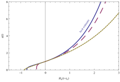
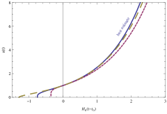
The scale factor and red shift corresponding to the transition from decelerated to accelerated expansion can be obtained as shown below. From the Hubble parameter (equation (10)) the derivative of $\dot{a}$ with respect to $a$ can be obtained as,

$$\frac{d\dot{a}}{da}=H_{0}\left[\left(\frac{\tilde{\zeta}_{1}-1}{2-\tilde{\zeta}_{2}}\right)\left(\frac{\tilde{\zeta}_{0}+\tilde{\zeta}_{12}-3}{\tilde{\zeta}_{12}-3}\right)a^{\frac{\tilde{\zeta}_{12}-3}{2-\tilde{\zeta}_{2}}}-\frac{\tilde{\zeta}_{0}}{\tilde{\zeta}_{12}-3}\right].$$ (19)

Equating this to zero, we obtain the transition scale factor $a_{T}$,

$$a_{T}=\left[\frac{\tilde{\zeta}_{0}\left(2-\tilde{\zeta}_{2}\right)}{\left(\tilde{\zeta}_{1}-1\right)\left(\tilde{\zeta}_{0}+\tilde{\zeta}_{12}-3\right)}\right]^{\frac{2-\tilde{\zeta}_{2}}{\tilde{\zeta}_{12}-3}}$$ (20)

and the corresponding transition red shift $z_{T}$ is,

$$z_{T}=\left[\frac{\tilde{\zeta}_{0}\left(2-\tilde{\zeta}_{2}\right)}{\left(\tilde{\zeta}_{1}-1\right)\left(\tilde{\zeta}_{0}+\tilde{\zeta}_{12}-3\right)}\right]^{-{\frac{2-\tilde{\zeta}_{2}}{\tilde{\zeta}_{12}-3}}}-1.$$ (21)

From equations (20) and (21), it is clear that if $\tilde{\zeta}_{0}+\tilde{\zeta}_{1}=1$, the transition from decelerated phase to accelerated phase occurs at $a_{T}=1$ and $z_{T}=0$, which corresponds to the present time of the universe. For the first case of limiting conditions of parameters with $\tilde{\zeta}_{0}>0$, the transition would takes place in the past if $\tilde{\zeta}_{0}+\tilde{\zeta}_{1}>1$ and in the future if $\tilde{\zeta}_{0}+\tilde{\zeta}_{1}<1$. For the second case of limiting conditions of parameters, that corresponds to $\tilde{\zeta}_{0}<0$, the above conditions are reversed such that transition would takes place in the future if $\tilde{\zeta}_{0}+\tilde{\zeta}_{1}>1$ and in the past if $\tilde{\zeta}_{0}+\tilde{\zeta}_{1}<1$. These are shown in figures 3 and 4 respectively, where we have plotted $\frac{d^{2}a}{dy^{2}}$ (equation 14) with $y$.

Age of the universe can be deduced from the scale factor equation (13) by equating it to zero. The time elapsed since the Big-Bang is,

$$t_{B}=t_{0}+\left(\frac{2-\tilde{\zeta}_{2}}{H_{0}\tilde{\zeta}_{0}}\right)\ln\left(1-\frac{\tilde{\zeta}_{0}}{3-\tilde{\zeta}_{12}}\right).$$ (22)

Hence, the age of the universe since Big-Bang is

$$Age\equiv t_{0}-t_{B}=-\left(\frac{2-\tilde{\zeta}_{2}}{H_{0}\tilde{\zeta}_{0}}\right)ln\left(1-\frac{\tilde{\zeta}_{0}}{3-\tilde{\zeta}_{12}}\right).$$ (23)

Figure 5: Plot of the age of the universe in Gyr with $H_{0}$ in units of $kms^{-1}Mpc^{-1}$ for the best fit values of the bulk viscous parameters. The plots are identical for the best estimated values of the parameters from both the limiting conditions. The point located in the figure corresponds to an age 10.5 Gyr for the best estimate value of $H_{0}$, obtained as $70.49kms^{-1}Mpc^{-1}$. The shaded region corresponds to the interval $H_{0}(55,75)kms^{-1}Mpc^{-1}$ and age $(10,15.8)$ Gyr, which are the permitted intervals for $H_{0}$ and age, derived using observations on Galactic globular clusters from the Hipparcos parallaxes [47].

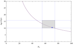
A plot of the age of the universe with $H_{0}$ for the best estimates of the bulk viscous parameters is shown in figure 5 (the evolution is the same for the best estimates from the two limiting conditions). The age of the universe corresponding to the best estimates of the present Hubble parameter is found to be $10.90$ Gyr and is marked in the plot. This value is less compared to the age deduced from CMB anisotropy data [46] and also that from the oldest globular clusters [47], which is around $12.9\pm 2.9$ Gyr. For comparison, we have also extracted the value of the Hubble parameter for the $\Lambda$CDM model using the same data set (see Table LABEL:tab:1 in section 7) from which the age of the universe is found to be around 13.85 Gyr. So compared to the age of the universe from globular clusters and the standard $\Lambda$CDM model, the present model, where the bulk viscous matter replaces the dark energy, predicts relatively a low age.

4 Cosmological parameters

4.1 Deceleration parameter

The results regarding the transition of the universe into the accelerated epoch discussed in the above section can be further verified by studying the evolution of the deceleration parameter $q,$ which is defined as,

$$q(a)=-\frac{\ddot{a}a}{\dot{a}^{2}}=-\frac{\ddot{a}}{a}\frac{1}{H^{2}}.$$ (24)

For the bulk viscous matter dominated universe, one can obtain using Friedmann equations,

$$\frac{\ddot{a}}{a}=-\frac{1}{6}\left[\rho_{m}-9H\left(\zeta_{0}+\zeta_{1}H+\zeta_{2}\left(\frac{\dot{H}}{H}+H\right)\right)\right].$$ (25)

Using the dimensionless bulk viscous parameters as defined in equation (9) and using equations (3) and (25), the deceleration parameter becomes,

$$q=\frac{1}{2}\left[1-\left(\frac{H_{0}}{H}\tilde{\zeta}_{0}+\tilde{\zeta}_{1}+\frac{\tilde{\zeta}_{2}}{H}\left(\frac{\dot{H}}{H}+H\right)\right)\right].$$ (26)

Substituting equations(8) and (10), we can obtain the deceleration parameter in terms of $a$, $\tilde{\zeta}_{0}$, $\tilde{\zeta}_{1}$ and $\tilde{\zeta}_{2}$ as,

$$q(a)=\frac{1}{2-\tilde{\zeta}_{2}}\left[1-\tilde{\zeta}_{1}-\frac{\tilde{\zeta}_{0}}{a^{\frac{\tilde{\zeta}_{12}-3}{2-\tilde{\zeta}_{2}}}\left[1+\frac{\tilde{\zeta}_{0}}{\tilde{\zeta}_{12}-3}\right]-\frac{\tilde{\zeta}_{0}}{\tilde{\zeta}_{12}-3}}\right].$$ (27)

In terms of red shift, the above equation becomes,

$$q(z)=\frac{1}{2-\tilde{\zeta}_{2}}[1-\tilde{\zeta}_{1}-\frac{\tilde{\zeta}_{0}}{(1+z)^{-\frac{\tilde{\zeta}_{12}-3}{2-\tilde{\zeta}_{2}}}[1+\frac{\tilde{\zeta}_{0}}{\tilde{\zeta}_{12}-3}]-\frac{\tilde{\zeta}_{0}}{\tilde{\zeta}_{12}-3}}].$$ (28)

Figure 6: Evolution of the deceleration parameter with red shift for the first limiting conditions of viscous parameters, $\tilde{\zeta}_{0}>0,\,\tilde{\zeta}_{0}+\tilde{\zeta}_{12}<3,\,\tilde{\zeta}_{12}<3,\,\tilde{\zeta}_{2}<2$. $q$ enters the negative region in the recent past if $\tilde{\zeta}_{0}+\tilde{\zeta}_{1}>1$, at present if $\tilde{\zeta}_{0}+\tilde{\zeta}_{1}=1$ and in the future if $\tilde{\zeta}_{0}+\tilde{\zeta}_{1}<1.$ Evolution of $q$ for the best estimated values of the bulk viscous parameters is also shown. The redshift at which the $q$ enters the negative region for the best estimated values of the bulk viscous parameters corresponds to $z_{T}=0.49^{+0.075}_{-0.057}.$

Figure 7: Evolution of the deceleration parameter with red shift for the second limiting conditions of viscous parameters, $\tilde{\zeta}_{0}<0,\,\tilde{\zeta}_{0}+\tilde{\zeta}_{12}>3,\,\tilde{\zeta}_{12}>3,\,\tilde{\zeta}_{2}>2.$ $q$ enters the negative region in the recent past if $\tilde{\zeta}_{0}+\tilde{\zeta}_{1}<1$, at present if $\tilde{\zeta}_{0}+\tilde{\zeta}_{1}=1$ and in the future if $\tilde{\zeta}_{0}+\tilde{\zeta}_{1}>1.$ Evolution of $q$ for the best estimated values of the bulk viscous parameters is also shown. The redshift at which the $q$ enters the negative region for the best estimated values of the bulk viscous parameters corresponds to $z_{T}=0.49^{+0.064}_{-0.066}.$

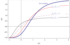
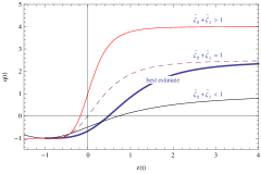
The variation of $q$ with $z$ for the two sets of limiting conditions of the viscous parameters are shown in figures 6 and 7. The evolution corresponding to the best estimates from both limiting conditions are identical as it is clear from the figures. When all the bulk viscous parameters are zero, the deceleration parameter $q=1/2$, which corresponds to a decelerating matter dominated universe with null bulk viscosity.

The present value of the deceleration parameter corresponds to $z=0$ or $a=1$ is,

$$q_{0}=q(a=1)=\frac{1-(\tilde{\zeta}_{0}+\tilde{\zeta}_{1})}{2-\tilde{\zeta}_{2}}.$$ (29)

This equation shows that for $\tilde{\zeta}_{0}+\tilde{\zeta}_{1}=1$, the deceleration parameter $q=0$. This implies that the transition into the accelerating phase would occur at the present time and is true for both the cases of the parameters.

For the first case of limiting conditions of the parameters (15) with $\tilde{\zeta}_{0}>0$ and $\tilde{\zeta}_{2}<2$, the current deceleration parameter $q_{0}<0$ if $\tilde{\zeta}_{0}+\tilde{\zeta}_{1}>1,$ implying that the present universe is in the accelerating epoch and it entered this epoch at an early stage. But $q_{0}>0$ if $\tilde{\zeta}_{0}+\tilde{\zeta}_{1}<1,$ implying that the present universe is decelerating and it will be entering the accelerating phase at a future time, see figure 6 which shows the behavior of $q$ with $z.$ For the best estimate of the bulk viscous parameters, the behavior of $q$ (figure 6) shows that the universe transit from decelerated to accelerated epoch at a recent past. The best estimate of the bulk viscous parameters corresponding to the first limiting case, equation 15 were extracted using the Supernova data and are $(\tilde{\zeta}_{0}=7.83,\tilde{\zeta}_{1}=-5.13,\tilde{\zeta}_{2}=-0.51)$ (see Table LABEL:tab:1), which indicate that $\tilde{\zeta}_{0}+\tilde{\zeta}_{1}>1.$ So the model predicts a universe which is accelerating at present and has entered this phase of accelerating expansion at a recent past.

For the second case of limiting conditions of the viscous parameters (16) with $\tilde{\zeta}_{0}<0$ and $\tilde{\zeta}_{2}>2$, the current deceleration parameter $q_{0}>0$ if $\tilde{\zeta}_{0}+\tilde{\zeta}_{1}>1,$ implies that the present universe is in the decelerating epoch and it will be entering the accelerating phase at a future time, see figure 7 which shows the behavior of $q$ with $z.$ But $q_{0}<0$ if $\tilde{\zeta}_{0}+\tilde{\zeta}_{1}<1,$ implying that the present universe is accelerating and it entered this phase at an early time. From the behavior of $q$ (figure 7) for the best estimate of the bulk viscous parameters corresponding to the second limiting condition, equation 16, it is clear that the transition of the universe from the decelerated to accelerated epoch was in the recent past. The best estimate of the bulk viscous parameters in this case are $(\tilde{\zeta}_{0}=-4.68,\tilde{\zeta}_{1}=4.67,\tilde{\zeta}_{2}=3.49)$ (see Table LABEL:tab:1), which indicate that $\tilde{\zeta}_{0}+\tilde{\zeta}_{1}<1.$ So, for this case also, the model predicts a universe which is accelerating at present and has entered this phase of accelerating expansion at a recent past.

These results confirm the earlier conclusion with respect to the behavior of $d^{2}a/dy^{2}$. For the best estimated values of the bulk viscous parameters, the present value of the deceleration parameter is found to be about $-0.68\pm 0.06$ and $-0.68^{+0.066}_{-0.05}$ corresponding to the first and second limiting conditions respectively (see equation (29)). This is comparable with the observational results on the present value of q, which is around $-0.64\pm 0.03$ [46, 48]. The transition red shift, at which $q$ enters the negative value region, corresponding to an accelerating epoch, is found to be $z_{T}=0.49^{+0.075}_{-0.057}$ for the first case of limiting conditions of the bulk viscous parameters and $z_{T}=0.49^{+0.064}_{-0.066}$ for the second case of limiting conditions of the bulk viscous parameters (see equation (21) and figures 6 and 7). An analysis of the $\Lambda$CDM model with combined SNe+CMB data gives the transition red shift range as $z_{T}=0.45-0.73$ [54]. So the transition red shift predicted by the present model is agreeing only with the lower limit of the corresponding $\Lambda$CDM range, and hence can be hardly considered as a good agreement.

4.2 Equation of state

An accelerated expansion of the universe is possible only if the effective equation of state parameter, $\omega<-1/3,$ or equivalently, $3\omega+1<0$. The equation of state can be obtained using [49],

$$\omega=-1-\frac{1}{3}\frac{d\ln h^{2}}{dx}$$ (30)

where $x=\ln a$ and $h=\frac{H}{H_{0}}$. Using equation (10) we get the equation of state as,

$$\omega=-1-\frac{2}{3(2-\tilde{\zeta}_{2})}\left[\tilde{\zeta}_{1}+\tilde{\zeta}_{2}-3+\frac{\tilde{\zeta}_{0}}{h}\right]$$ (31)

The present value of the equation of state parameter $\omega_{0}$, can be obtained by taking $h=1$. The condition for acceleration of the present universe can then be represented as,

$$3\omega_{0}+1=-2\left(\frac{\tilde{\zeta}_{0}+\tilde{\zeta}_{1}-1}{2-\tilde{\zeta}_{2}}\right)<0$$ (32)

For the first case of parameters with $\tilde{\zeta}_{0}>0$, $\tilde{\zeta}_{2}<2$, this condition is satisfied if $\tilde{\zeta}_{0}+\tilde{\zeta}_{1}>1$ and for the second case with $\tilde{\zeta}_{0}<0$, $\tilde{\zeta}_{2}>2$, this will be satisfied if $\tilde{\zeta}_{0}+\tilde{\zeta}_{1}<1$. These conditions are compatible with that arrived in the analysis of deceleration parameter in section 4.1.

Figure 8: Evolution of the equation of state parameter with red shift for the best estimates of the bulk viscous parameters. It is found that the evolution of $\omega$ are identical for the best estimates from both the limiting conditions.

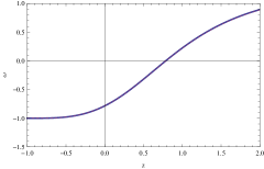
The evolution of the equation of state parameter with red shift for both the sets of the best fit values of the bulk viscous parameters are found to be identical and is shown in figure 8. It is clear from the figure that as $z\rightarrow-1$ ($a\rightarrow\infty$), $\omega\rightarrow-1$ in the future which corresponds to the de Sitter universe and also coincides with that of the future behavior of the $\Lambda$CDM model [50], and also resembles the behavior of some scalar field models [6]. Since it is not crossing the phantom divide $\omega\leq-1$, the model is free from big rip singularity or little rip [51]. The present value of the equation of state parameter is around $\omega_{0}\sim-0.78^{+0.03}_{-0.045}$ and $\omega_{0}\sim-0.78^{+0.037}_{-0.043}$ for the best estimate of viscosity parameters corresponding to the first and second limiting conditions, respectively. This value is comparatively higher than that predicted by the joint analysis of WMAP+BAO+$H_{0}$+SN data, which is around $-0.93$ [52, 53].

4.3 Evolution of matter density

From the Friedmann equation (3) and the Hubble parameter (10) we obtain the mass density parameter $\Omega_{m}$ as,

$$\Omega_{m}(a)=\left[a^{\frac{\tilde{\zeta}_{12}-3}{2-\tilde{\zeta}_{2}}}\left[1+\frac{\tilde{\zeta}_{0}}{\tilde{\zeta}_{12}-3}\right]-\frac{\tilde{\zeta}_{0}}{\tilde{\zeta}_{12}-3}\right]^{2}$$ (33)

Figure 9: Evolution of the mass density parameter with scale factor for the best estimated values of the bulk viscous parameters. It is found that the variation of the mass density coincides for the best estimated values from the two limiting conditions.

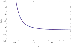
where, $\Omega_{m}=\frac{\rho_{m}}{\rho_{crit}}$ and $\rho_{crit}=3H_{0}^{2}$ is the critical density. If $\tilde{\zeta}_{0}=\tilde{\zeta}_{1}=\tilde{\zeta}_{2}=0$, the mass density parameter reduces to $\Omega_{m}\sim a^{-3}$, which corresponds to the matter dominated universe with null bulk viscosity. The evolution of the mass density parameter for the best estimated values corresponding to the two limiting conditions are shown in figure 9 and it is clear that their evolutions are coinciding with each other. As $a\rightarrow 0$, the matter density diverges. Figure 9 also indicating the same, which is a clear indication of the existence of the Big-Bang at the origin of the universe.

4.4 The curvature scalar

The curvature scalar is the parameter used to confirm the presence of singularities in the model. For a flat universe, the curvature scalar is defined as,

$$R=6\left[\frac{\ddot{a}}{a}+H^{2}\right].$$ (34)

Using equations (8), (9), (10) and (25), we obtain the curvature scalar as,

$$\begin{split}R(a)=&\frac{6H_{0}^{2}}{(2-\tilde{\zeta}_{2})(\tilde{\zeta}_{12}-3)^{2}}[2\tilde{\zeta}_{0}^{2}(2-\tilde{\zeta}_{2})+(\tilde{\zeta}_{0}+\tilde{\zeta}_{12}-3)\\ &a^{\frac{\tilde{\zeta}_{12}-3}{2-\tilde{\zeta}_{2}}}[(\tilde{\zeta}_{1}-\tilde{\zeta}_{2}+1)(\tilde{\zeta}_{0}+\tilde{\zeta}_{12}-3)a^{\frac{\tilde{\zeta}_{12}-3}{2-\tilde{\zeta}_{2}}}-\\ &\tilde{\zeta}_{0}(\tilde{\zeta}_{1}-3\tilde{\zeta}_{2}+5)]].\end{split}$$ (35)

Figure 10: Evolution of the curvature scalar with scale factor for the best estimate parameters. It is found that the evolution of the curvature scalar are identical for the best estimated values from the two limiting conditions.

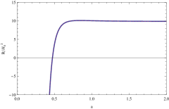
From the above equation it is clear that as $a\rightarrow 0$, $R\rightarrow\infty.$ The evolution of the curvature scalar for both the cases of best fit of the parameters coincides with each other as shown in figure 10. The behavior of $R$ shows that the curvature scalar diverges as $a\to 0.$ This indicates the existence of Big-Bang at the origin of the universe.

5 Entropy and second law of thermodynamics

In the FLRW space-time, the law of generation of the local entropy is given as [30]

$$T\nabla_{\nu}s^{\nu}=\zeta(\nabla_{\nu}u^{\nu})^{2}=9H^{2}\zeta$$ (36)

where $T$ is the temperature and $\nabla_{\nu}s^{\nu}$ is the rate of generation of entropy in unit volume. The second law of thermodynamics will be satisfied if,

$$T\nabla_{\nu}s^{\nu}\geq 0$$ (37)

which implies from equation (36) that

$$\zeta\geq 0.$$ (38)

Using equations (8) and (10), the total dimensionless bulk viscous parameter (equation (6)), can be obtained as

$$\tilde{\zeta}(a)=\frac{1}{2-\tilde{\zeta}_{2}}\left[2\tilde{\zeta}_{0}+\left(2\tilde{\zeta}_{1}-\tilde{\zeta}_{2}\right)\frac{H}{H_{0}}\right],$$ (39)

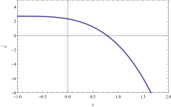
where $\tilde{\zeta}=\frac{3\zeta}{H_{0}}$, the total dimensionless bulk viscous parameter. We have studied the evolution of $\tilde{\zeta}$ using the best estimated values for both cases of parameters and found that the evolution of the total bulk viscous parameter are coinciding for both the cases as shown in figure 11. The figure also shows that the total bulk viscous coefficient is evolving continuously from the negative value region to a positive region. When $z\leq 0.8$, the total bulk viscous parameter becomes positive. This means that the rate of entropy production is negative in the early epoch and positive in the later epoch. Hence the local second law is violated in the early epoch and is obeyed in the later epoch. This seems to be a drawback of the present model. However, it can be considered as a theoretical possibility [55]. In an absolute way the status of the second law of thermodynamics should be considered along with the accounting of the entropy generation from the horizon. In that circumstances, the second law becomes the generalized second law of thermodynamics, which state that the total entropy of the fluid components of the universe plus that of the horizon should never decrease [56, 57]. In the present model this means the rate of entropy change of the bulk viscous matter and that of the horizon must be greater than zero.

$$\frac{d}{dt}\left(S_{m}+S_{h}\right)\geq 0$$ (40)

where, $S_{m}$ is the entropy of the matter and $S_{h}$ is that of the horizon. For a flat FLRW universe, the apparent horizon radius is given as [58]

$$r_{A}=\frac{1}{H}.$$ (41)

The entropy associated to the apparent horizon is [60],

$$S_{h}=2\pi A=8\pi^{2}r_{A}^{2}$$ (42)

where $A=4\pi r_{A}^{2}$ is the area of the apparent horizon and we have assumed $8\pi G=1$. Using the first Friedmann equation and equations (2), (5), (7) and (41), we obtain,

$$\dot{r}_{A}=\frac{1}{2}r_{A}^{3}H\left[-H(\tilde{\zeta}_{0}H_{0}+\tilde{\zeta}_{1}H+\tilde{\zeta}_{2}(\frac{\dot{H}}{H}+H))+\rho_{m}\right]$$ (43)

The temperature of the apparent horizon can be defined as [59]

$$T_{h}=\frac{1}{2\pi r_{A}}\left(1-\frac{\dot{r}_{A}}{2Hr_{A}}\right).$$ (44)

Using equations (42), (43) and (44), we arrive

$$\begin{split}T_{h}\dot{S}_{h}=4\pi r_{A}^{3}H\left[\rho_{m}-H(\tilde{\zeta}_{0}H_{0}+\tilde{\zeta}_{1}H+\tilde{\zeta}_{2}(\frac{\dot{H}}{H}+H))\right]\\ \left[1-\frac{\dot{r}_{A}}{2Hr_{A}}\right].\end{split}$$ (45)

Figure 11: Evolution of the total dimensionless bulk viscous parameter with respect to the red shift for the best estimated values corresponding to the two limiting conditions. $\tilde{\zeta}$ is positive for $z\leq 0.8.$

The change in entropy of the viscous matter inside the apparent horizon can be obtained using the Gibbs equation,

$$T_{m}dS_{m}=d(\rho_{m}V)+P^{*}dV$$ (46)

where $T_{m}$ is the temperature of the bulk viscous matter, $V=\frac{4}{3}\pi r_{A}^{3}$ is the volume enclosed by the apparent horizon. Using equations (2) and (7), the Gibbs equation becomes

$$T_{m}dS_{m}=Vd\rho_{m}+(\rho_{m}-H(\tilde{\zeta}_{0}H_{0}+\tilde{\zeta}_{1}H+\tilde{\zeta}_{2}(\frac{\dot{H}}{H}+H)))dV.$$ (47)

Under equilibrium conditions, the temperature $T_{m}$ of the viscous matter and that of the horizon $T_{h}$ are equal, $T_{m}=T_{h}$. Then the Gibbs equation (47) becomes

$$\begin{split}T_{h}\dot{S}_{m}=4\pi r_{A}^{3}H\left[H(\tilde{\zeta}_{0}H_{0}+\tilde{\zeta}_{1}H+\tilde{\zeta}_{2}(\frac{\dot{H}}{H}+H)-\rho_{m})\right]\\ +4\pi r_{A}^{2}\dot{r}_{A}\left[\rho_{m}-H(\tilde{\zeta}_{0}H_{0}+\tilde{\zeta}_{1}H+\tilde{\zeta}_{2}(\frac{\dot{H}}{H}+H))\right].\end{split}$$ (48)

Adding equations (45) and (48), we get

$$T_{h}(\dot{S}_{h}+\dot{S}_{m})=\frac{A}{4}Hr_{A}^{3}[\rho_{m}-H(\tilde{\zeta}_{0}H_{0}+\tilde{\zeta}_{1}H+\tilde{\zeta}_{2}({\dot{H}\over H}+H))]^{2}.$$ (49)

$A$, the area of the apparent horizon, $H$, the Hubble parameter and the radius $r_{A}$ are always positive, therefore, $\dot{S}_{h}+\dot{S}_{m}\geq 0$ for a given temperature. This means that the generalized second law (GSL) is always valid. Hence the decrease in the entropy of the viscous matter is compensated by the increase in the entropy of the horizon. Even though the violation of the local second law of thermodynamics can be considered as a draw back of this model, the validity of the Generalized second law for the entire causal region of the universe may safe guard the model.

6 Statefinder analysis

In this section, we present our analysis on comparing the present model with other standard models of dark energy. We have used the statefinder parameter diagnostic introduced by Sahni et al [63]. The statefinder is a geometrical diagnostic tool which allows us to characterize the properties of dark energy in a model-independent manner. The statefinder parameters $\{r,s\}$ are defined as,

$$r=\frac{\dddot{a}}{aH^{3}},\ \ \ \ \ \ s=\frac{r-1}{3\left(q-\frac{1}{2}\right)}.$$ (50)

In terms of $h=\frac{H}{H_{0}}$, $r$ and $s$ can be written as

$$r=\frac{1}{2h^{2}}\frac{d^{2}h^{2}}{dx^{2}}+\frac{3}{2h^{2}}\frac{dh^{2}}{dx}+1$$ (51)

$$s=-\frac{\frac{1}{2h^{2}}\frac{d^{2}h^{2}}{dx^{2}}+\frac{3}{2h^{2}}\frac{dh^{2}}{dx}}{\frac{3}{2h^{2}}\frac{dh^{2}}{dx}+\frac{9}{2}}.$$ (52)

Using the expression for $h$ from equation (10), these parameters become,

$$\begin{split}r=\frac{(\tilde{\zeta}_{0}+\tilde{\zeta}_{12}-3)(\tilde{\zeta}_{12}-3)}{h^{2}(2-\tilde{\zeta}_{2})^{2}}a^{\frac{\tilde{\zeta}_{12}-3}{2-\tilde{\zeta}_{2}}}[2h+\frac{\tilde{\zeta}_{0}}{\tilde{\zeta}_{12}-3}]+\\ \frac{3(\tilde{\zeta}_{0}+\tilde{\zeta}_{12}-3)}{h(2-\tilde{\zeta}_{2})}a^{\frac{\tilde{\zeta}_{12}-3}{2-\tilde{\zeta}_{2}}}+1\end{split}$$ (53)

$$s=\frac{\frac{(\tilde{\zeta}_{0}+\tilde{\zeta}_{12}-3)(\tilde{\zeta}_{12}-3)}{h^{2}(2-\tilde{\zeta}_{2})^{2}}a^{\frac{\tilde{\zeta}_{12}-3}{2-\tilde{\zeta}_{2}}}[2h+\frac{\tilde{\zeta}_{0}}{\tilde{\zeta}_{12}-3}]+\frac{3(\tilde{\zeta}_{0}+\tilde{\zeta}_{12}-3)}{h(2-\tilde{\zeta}_{2})}a^{\frac{\tilde{\zeta}_{12}-3}{2-\tilde{\zeta}_{2}}}}{\frac{3(\tilde{\zeta}_{0}+\tilde{\zeta}_{12}-3)}{h(2-\tilde{\zeta}_{2})}a^{\frac{\tilde{\zeta}_{12}-3}{2-\tilde{\zeta}_{2}}}+\frac{9}{2}}.$$ (54)

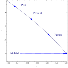
The above equations show that in the limit $a\to\infty$, the statefinder parameters $\{r,s\}\to\{1,0\}$, a value corresponding to the $\Lambda$CDM model of the universe. So the present model resembles the $\Lambda$CDM model in the future. The $\{r,s\}$ plane trajectory of the model is shown in figure 12. The trajectories are coinciding with each other for the best estimates from both the sets of the limiting conditions of the parameters. The trajectory in the $\{r,s\}$ plane are lying in the region $r>1,s<0$, a feature similar to the generalized Chaplygin gas model of dark energy [64]. The present model can also be discriminated from the Holographic dark energy model with event horizon as the I.R. cut off, in which the $r-s$ evolution starts from a region $r\sim 1,s\sim 2/3$ and end on the $\Lambda$CDM point [61]. The present position of the universe dominated by the bulk viscous matter is noted in the plot and it corresponds to $\{r_{0},s_{0}\}=\{1.25,-0.07\}$. This means that the present model is distinguishably different from the $\Lambda$CDM model.

Figure 12: The evolution of the model in the r-s plane for the best estimates of the parameters. The curves are coinciding with each other for the best estimated values of the parameters from both the limiting conditions.

7 Parameter estimation using type Ia Supernovae data

In this section we have obtained best fit of the parameters, $\tilde{\zeta}_{0}$, $\tilde{\zeta}_{1}$, $\tilde{\zeta}_{2}$ and $H_{0}$ using the type Ia Supernovae observations. The goodness-of-fit of the model is obtained by the $\chi^{2}$-minimization. We did the statistical analysis using the Supernova Cosmology Project (SCP) “Union” SNe Ia data set [62], composed of 307 type Ia Supernovae from 13 independent data sets.

In a flat universe, the luminosity distance $d_{L}$ is defined as

$$d_{L}(z,\tilde{\zeta}_{0},\tilde{\zeta}_{1},\tilde{\zeta}_{2},H_{0})=c(1+z)\int_{0}^{z}\frac{dz^{\prime}}{H(z^{\prime},\tilde{\zeta}_{0},\tilde{\zeta}_{1},\tilde{\zeta}_{2},H_{0})}$$ (55)

where $H(z,\tilde{\zeta}_{0},\tilde{\zeta}_{1},\tilde{\zeta}_{2},H_{0})$ is the Hubble parameter and $c$ is the speed of light. The theoretical distance moduli $\mu_{t}$ for the k-th Supernova with redshift $z_{k}$ is given as,

$$\begin{split}\mu_{t}(z_{k},\tilde{\zeta}_{0},\tilde{\zeta}_{1},\tilde{\zeta}_{2},H_{0})&=m-M\\ &=5\log_{10}[\frac{d_{L}(z_{k},\tilde{\zeta}_{0},\tilde{\zeta}_{1},\tilde{\zeta}_{2},H_{0})}{Mpc}]+25\end{split}$$ (56)

where, $m$ and $M$ are the apparent and absolute magnitudes of the SNe respectively. Then we can construct $\chi^{2}$ function as,

$$\chi^{2}(\tilde{\zeta}_{0},\tilde{\zeta}_{1},\tilde{\zeta}_{2},H_{0})\equiv\sum^{n}_{k=1}\frac{\left[\mu_{t}(z_{k},\tilde{\zeta}_{0},\tilde{\zeta}_{1},\tilde{\zeta}_{2},H_{o})-\mu_{k}\right]^{2}}{\sigma_{k}^{2}}$$ (57)

where $\mu_{k}$ is the observational distance moduli for the k-th Supernova, $\sigma_{k}^{2}$ is the variance of the measurement and $n$ is the total number of data, here $n=307$. The $\chi^{2}$ function, thus obtained is then minimized to obtain the best estimate of the parameters, $\tilde{\zeta}_{0}$, $\tilde{\zeta}_{1}$, $\tilde{\zeta}_{2}$ and $H_{0}$. From the behavior of scale factor and other cosmological parameters, we found that there exists two possible sets of conditions which describes a universe having a Big-Bang at the origin, then entering an early stage of decelerated expansion followed by acceleration. These two sets of conditions are mentioned in section 3. We have used these two conditions separately in minimizing the $\chi^{2}$ function. This leads to two sets of values for the best estimates of the parameters $\tilde{\zeta}_{0}$, $\tilde{\zeta}_{1}$, $\tilde{\zeta}_{2}$ but $H_{0}$ is same in both the cases. In addition to $H_{0}$, the other cosmological parameters, scale factor, deceleration parameter, equation of state parameter, matter density and curvature scalar are all showing identical behavior for both the sets of best fit of parameters. The values of the parameters are given in Table LABEL:tab:1. Inorder to compare the results of the present model, we have also estimated the values for $\Lambda$CDM model using the same data set and the results are also shown in Table LABEL:tab:1. We find that the values of $H_{0}$ and Goodness-of-fit $\chi^{2}_{d.o.f}$ for $\Lambda$CDM model are very close to those obtained from the present bulk viscous model. The value of the present Hubble parameter, $H_{0}$ for both the cases of parameters are found to be $70.49$ $kms^{-1}Mpc^{-1}$, which is in close agreement with the corresponding WMAP value ($H_{0}=70.5\pm 1.3$ $kms^{-1}Mpc^{-1}$) [48].

Table 1: Best estimates of the Bulk viscous parameters and $H_{0}$ and also $\chi^{2}$ minimum value for the two cases of the bulk viscous matter dominated universe. $\chi^{2}_{d.o.f}=\frac{\chi^{2}_{min}}{n-m}$, where $n=307$, the number of data and $m=3$, the number of parameters in the model. For the best estimation we have use SCP “Union” 307 SNe Ia data sets. We have also shown the best estimates for the $\Lambda$CDM model for comparison, where $\Omega_{m0}$ is the present mass density parameter. The subscript d.o.f stands for degrees of freedom.

Model $\rightarrow$	Bulk viscous model with $\tilde{\zeta}_{0}>0,\tilde{\zeta}_{0}+\tilde{\zeta}_{12}<3,\tilde{\zeta}_{12}<3,\tilde{\zeta}_{2}<2$	Bulk viscous model with $\tilde{\zeta}_{0}<0,\tilde{\zeta}_{0}+\tilde{\zeta}_{12}>3,\tilde{\zeta}_{12}>3,\tilde{\zeta}_{2}>2$	$\Lambda$CDM
$\tilde{\zeta}_{0}$	7.83	-4.68	-
$\tilde{\zeta}_{1}$	$-5.13^{+0.056}_{-0.060}$	$4.67^{+0.04}_{-0.03}$	-
$\tilde{\zeta}_{2}$	$-0.51^{+0.13}_{-0.14}$	$3.49^{+0.089}_{-0.071}$	-
$\Omega_{m0}$	1	1	0.316
$H_{0}$	70.49	70.49	70.03
$\chi^{2}_{min}$	310.54	310.54	311.93
$\chi^{2}_{d.o.f}$	1.02	1.02	1.02

Figure 13: Confidence intervals for the parameters $(\tilde{\zeta}_{1},\tilde{\zeta}_{2})$, for the first set of limiting conditions, for the bulk viscous matter dominated universe using the SCP “Union” data set composed of 307 data points. The best estimated values of the parameters are $\tilde{\zeta}_{1}=-5.13^{+0.056}_{-0.06}$ and $\tilde{\zeta}_{2}=-0.51^{+0.13}_{-0.14}$ and are indicated by the point. The confidence intervals shown corresponds to 68.3%, 95.4%, 99.73% and 99.99% of probabilities.

Figure 14: Confidence intervals for the parameters $(\tilde{\zeta}_{1},\tilde{\zeta}_{2})$, for the second set of limiting conditions, for the bulk viscous matter dominated universe using the SCP “Union” data set composed of 307 data points. The best estimated values of the parameters are $4.67^{+0.04}_{-0.03}$ and $3.49^{+0.089}_{-0.071}$ and are indicated by the point. The confidence intervals shown corresponds to 68.3%, 95.4%, 99.73% and 99.99% of probabilities.

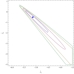
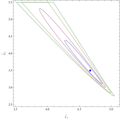
We have constructed the confidence interval plane for the bulk viscous parameters $(\tilde{\zeta}_{1},\tilde{\zeta}_{2})$ by keeping $\tilde{\zeta}_{0}$ as a constant equal to its best estimated value obtained by minimizing the $\chi^{2}$ function. From figure 13, corresponding to the first set of limiting conditions, and figure 14, corresponding to the second set of limiting conditions, it is seen that the fitting of the confidence intervals corresponding to $99.73\%$ and $99.99\%$ probabilities are poor. But the confidence intervals corresponding to $68.3\%$ and $95.4\%$ probabilities are showing a fairly good behavior. From the equation of the total bulk viscous coefficient (equation (39)) it can be easily verified that the present value of the total viscosity coefficient is positive in the region of confidence interval.

For the first case of parameters with $\tilde{\zeta}_{0}>0$, it is found that $\tilde{\zeta}_{1}=-5.13^{+0.056}_{-0.06}$ and $\tilde{\zeta}_{2}=-0.51^{+0.13}_{-0.14}$, for $\tilde{\zeta}_{0}=7.83$ with $68.3\%$ probability. In the second case with $\tilde{\zeta}_{0}<0$, the values of $\tilde{\zeta}_{1}$ and $\tilde{\zeta}_{2}$ are obtained as $4.67^{+0.04}_{-0.03}$ and $3.49^{+0.089}_{-0.071}$, respectively, for $\tilde{\zeta}_{0}=-4.68$ with $68.3\%$ probability.

8 Conclusions

In this paper, we have carried out a study of the bulk viscous matter dominated universe with bulk viscosity of the form $\zeta=\zeta_{0}+\zeta_{1}\frac{\dot{a}}{a}+\zeta_{2}\frac{\ddot{a}}{\dot{a}}.$ This model automatically solves the coincidence problem because the bulk viscous matter simultaneously represents dark matter and dark energy and causes recent acceleration. We have identified two possible limiting conditions for bulk viscous parameters where the universe begins with a Big-Bang, followed by decelerated expansion in the early times and then making a transition to the accelerated epoch at recent past. These conditions corresponds to $(\tilde{\zeta}_{0}>0,\tilde{\zeta}_{0}+\tilde{\zeta}_{12}<3,\tilde{\zeta}_{12}<3,\tilde{\zeta}_{2}<2)$ and $(\tilde{\zeta}_{0}<0,\tilde{\zeta}_{0}+\tilde{\zeta}_{12}>3,\tilde{\zeta}_{12}>3$, $\tilde{\zeta}_{2}>2).$

In constraining the parameter we have used SCP “Union” type Ia Supernova data set. We have computed the minimum values of $\chi^{2}$ function by degrees of freedom ($\chi^{2}_{d.o.f}$) for both cases of limiting conditions of the bulk viscous parameters and are found to be very near to one, indicating a reasonable goodness-of-fit. We have evaluated the best fit values of the three parameters, $(\tilde{\zeta}_{0},\tilde{\zeta}_{1},\tilde{\zeta}_{2})$ simultaneously for both cases of limiting conditions of the parameters and are shown in Table LABEL:tab:1.

For both cases of the best estimate of the bulk viscous parameters, the evolution of the cosmological parameters: the scale factor, deceleration parameter, the equation of state parameter, matter density, curvature scalar are all found to be identical. So these two sets of best estimated values for the parameters cannot be distinguished by using the conventional cosmological parameters. By doing a phase space analysis, it may be possible to distinguish between these two limiting conditions so as to remove the apparent degeneracy in the best estimated values of bulk viscous coefficient, such a work is in progress and will be reported else where.

From the evolution of scale factor, it is found that for the first limiting conditions of bulk viscous parameters, the transition into the accelerating epoch would be in the recent past if $\tilde{\zeta}_{0}+\tilde{\zeta}_{1}>1$. On the other hand if $\tilde{\zeta}_{0}+\tilde{\zeta}_{1}<1$, the transition takes place in the future and if, $\tilde{\zeta}_{0}+\tilde{\zeta}_{1}=1$, the transition takes place at the present time. For the second limiting conditions of parameters the above conditions are getting reversed such that when $\tilde{\zeta}_{0}+\tilde{\zeta}_{1}>1$, the transition will takes place in the future, when $\tilde{\zeta}_{0}+\tilde{\zeta}_{1}<1$, the transition would occur in the recent past and when $\tilde{\zeta}_{0}+\tilde{\zeta}_{1}=1$, the transition takes place at the present time.

We have also estimated the present age of the universe and found to be around $10.90$ Gyr for the best estimates of the parameters. Compared to the age predicted from oldest galactic globular clusters ($12.9\pm 2.9$ Gyr), the present value is relatively less, but just within the concordance limit.

The evolution of the deceleration parameter shows that the transition from the decelerated to the accelerated epoch occurs at the present time, corresponding to $q=0$ if $\tilde{\zeta}_{0}+\tilde{\zeta}_{1}=1$, for both sets of limiting conditions of the parameters. The transition would be in the recent past, corresponds to $q<0$ at present, if $\tilde{\zeta}_{0}+\tilde{\zeta}_{1}>1$ for the first set of limiting conditions and $\tilde{\zeta}_{0}+\tilde{\zeta}_{1}<1$, for the second set. The transition into the accelerating epoch will be in the future, corresponds to $q>0$ at present if $\tilde{\zeta}_{0}+\tilde{\zeta}_{1}<1$ for the first set of limiting conditions of the parameters and $\tilde{\zeta}_{0}+\tilde{\zeta}_{1}>1$ for the second set. However, for the best estimates of viscous parameters from both the limiting conditions, the behavior of the deceleration parameters are identical. It is found that for the best estimates, the universe entered the accelerating phase in the recent past at a red shift $z_{T}=0.49^{+0.075}_{-0.057}$ for the first limiting conditions and $z_{T}=0.49^{+0.064}_{-0.066}$ for the second limiting conditions. This is found to be agreeing only with the lower limit of the corresponding $\Lambda$CDM range, $z_{T}=0.45-0.73$ [54]. The present value of the deceleration parameter is found to be about $-0.68^{+0.06}_{-0.06}$ and $-0.68^{+0.066}_{-0.05}$ for the two cases respectively and is comparable with the observational results which is around $-0.64\pm 0.03.$

We have analyzed the equation of state parameter for the best estimates of the bulk viscous parameters only. The equation of state parameter $\omega\to-1$ as $z\to-1,$ which means that the bulk viscous matter dominated universe behaves like the de Sitter universe in future. It is also clear that the equation of state parameter of this model doesn’t cross the phantom divide and thereby, free from big rip singularity. The present value of the equation of state parameter is around $-0.78^{+0.03}_{-0.045}$ and $-0.78^{+0.037}_{-0.043}$ for the best fit of viscosity parameters corresponding to the two limiting conditions respectively. This value is comparatively higher than that predicted by the joint analysis of WMAP+BAO+H0+SN data, which is around -0.93 [52, 53].

From the expression for matter density, it is clear that it diverges as the scale factor tends to zero, which indicates the existence of Big-Bang at the origin. This is further confirmed by obtaining the curvature scalar which also becomes infinity at the origin.

The evolution of the total bulk viscous parameter is studied for the best estimates of the bulk viscous parameter corresponding to equations (15) and (16). In the initial epoch of expansion, the total bulk viscosity is found to be negative and hence violating the local second law of thermodynamics. But it become positive from $z\leq 0.8$, from there onwards the local second law is satisfied. However we found that the generalized second law is satisfied throughout the evolution of the universe.

Since the model predicts the late acceleration of the universe as like the standard forms of dark energy, we have analyzed the model using statefinder parameters to distinguish it from other standard dark energy models especially from $\Lambda$CDM model. The evolution of the present model in the $\{r,s\}$ plane is shown in figure 12 and it shows that the evolution of the {r,s} parameter is in such a way that $r>1,s<0$, a feature similar to the Chaplygin gas model. The present position of the bulk viscous model in the r-s plane corresponds to $\{r_{0},s_{0}\}=\{1.25,-0.07\}$. Hence the model is distinguishably different from the $\Lambda$CDM model.

Even though the model predicts the late acceleration, it failed particularly in predicting the age of the universe and equation of state parameter. It also fails with regard to the validity of the local second law of thermodynamics even though the generalized second law is satisfied. A similar model was studied in reference [29], where the authors have ruled out the possibility of bulk viscous dark matter as a candidate of dark energy. But their analysis is essentially a two parameter one since they took either $\tilde{\zeta}_{1}$ or $\tilde{\zeta}_{2}$ as zero with $\tilde{\zeta}_{0}>0.$ In the present work we have evaluated $\tilde{\zeta}_{0}$, $\tilde{\zeta}_{1}$ and $\tilde{\zeta}_{2}$ simultaneously and found that there is a possibility for $\tilde{\zeta}_{0}<0$ which gives a similar evolution of the cosmological parameters as with $\tilde{\zeta}_{0}>0$. A crucial test of this model is whether it predict the conventional radiation dominated phase in the early universe. For this, one has to study the phase space structure of this model and that will be a subject of our future study. Such a study may also remove the apparent degeneracy in the best estimated values of the bulk viscous parameters.

In reference [21], the authors have considered a unified model for the dark sectors with a single component universe consisting of bulk viscous dark matter, with the viscosity coefficient as a function of density alone. They have found that in the background level the model predicts an early deceleration and a late acceleration. They also have analyzed the evolution of the first order density perturbation. Regarding the density perturbation growth, the authors have shown that for $\zeta(\rho)=\alpha\rho^{m}$, with $m=-0.4$ and $\alpha\propto 0.236$, the density perturbations behave drastically different from that of cold dark matter in such a way that the presence of the viscosity becomes significant and rapidly damped out the density perturbations at small scales. This also causes the decay of gravitational potential and hence modifies the large scale CMB spectrum. The authors have pointed out that if $\zeta$ becomes a function of $H$ and $\dot{H}$, like our case, the situation becomes more complex and would enhance the damping of the perturbation growth. A similar study was also carried out in reference [66]. In this, the authors have considered the ansatz $\zeta\propto\rho^{\nu}$ for the coefficient of bulk viscosity and with $\nu=\frac{1}{2}$, the model mimics the $\Lambda$CDM background evolution. They have shown that the viscous dark fluids contribute to ISW Effect and thereby suppressing the structure growth at small scales.

An important effect with which the model is to be contrasted is the Integrated Sachs-Wolfe effect(ISW). The ISW Effect is the change in the energy of a CMB photon as it passes through the evolving gravitational potential wells [65]. For large time, the behaviour of $a$ tends to that of the $\Lambda$CDM model for which $\phi\sim 1+z$. So compared to the time of decoupling ($z\sim 1090$), the potential will be diluted at later times which consequentially causes the ISW effect. In the appendix below, we have presented a brief argument regarding the ISW effect in the present model.

Acknowledgment
The authors are thankful to the referee for the critical comments which helped to improve the manuscript. The authors are also thankful to Prof. Sahni for the valuable discussions. One of the authors (TKM) is thankful to IUCAA, Pune for the hospitality, where part of the work has been carried out. The author (AS) is thankful to DST for giving financial support through INSPIRE fellowship.

Appendix
ISW effect
Viscous dark matter will, in general, resist to the density perturbations. Consequently it will dilute the gravitational potential at the perturbed regions. This will subsequently affect the CMB radiation and leads to ISW effect.

The ISW Effect is the change in the energy of a CMB photon as it passes through the evolving gravitational potential wells. It is obtained as

$$(\frac{\Delta T}{T})_{ISW}=2\int^{\eta_{0}}_{\eta_{r}}\Phi^{\prime}[(\eta_{0}-\eta)\bf{\hat{n}},\eta]d\eta$$ (58)

where $\hat{n}$ is the photon trajectory and $\eta_{0}$ is the conformal time today and $\eta_{r}$ is the conformal time at recombination, $\Phi$ is the gravitational potential and prime represents derivative with respect to the conformal time.

So the first step towards the calculation of the ISW Effect is to obtain the evolution of gravitational potential in an expanding universe. This can be obtained from Einstein’s equation by taking care of the perturbations. Viscous dark matter may cause a fast decay of gravitational potential which modifies the CMB spectrum.

In Fourier space, the gravitational potential takes the form [67]

$$\Phi=\frac{3}{2}\frac{\Omega_{mo}}{a}(\frac{H_{0}}{k})^{2}\delta(k,\eta)$$ (59)

where density perturbation, $\delta(k,\eta)=G(\eta)\delta(k,0)$. $G(\eta)$ is the growth factor which is related to the Hubble parameter as,

$$G(\eta)\propto\frac{H(\eta)}{H_{0}}\int_{z(\eta)}^{\infty}dz^{\prime}(1+z^{\prime})(\frac{H_{0}}{H(z^{\prime})})^{3}$$ (60)

In matter dominated universe, $G\propto a$, so $\Phi$ remains a constant, hence no ISW effect.

In our model, by considering the bulk viscous coefficient $\zeta=\zeta_{0}+\zeta_{1}\frac{\dot{a}}{a}+\zeta_{2}\frac{\ddot{a}}{\dot{a}}$, the Hubble parameter evolves as equation (10). By using this relation, the integral in the growth factor becomes hypergeometric function. For simplification, let us consider the case when $a$ is large, then $H\propto a^{\frac{\tilde{\zeta}_{1}+\tilde{\zeta}_{2}-3}{2-\tilde{\zeta}_{2}}}$. Then the growth factor becomes,

$$G\propto(1+z)^{\frac{\tilde{\zeta}_{1}+\tilde{\zeta}_{2}-3}{2-\tilde{\zeta}_{2}}}\left(\frac{(2-\tilde{\zeta}_{2})z^{\frac{-3\tilde{\zeta}_{1}+\tilde{\zeta}_{2}+5}{2-\tilde{\zeta}_{2}}}}{-3\tilde{\zeta}_{1}-\tilde{\zeta}_{2}+5}\right)$$ (61)

So, potential becomes $\Phi\propto z^{8.34}(1+z)^{4.45}$ (by using extracted parameter values). From the last scattering surface, which corresponds to $z=1091$, to the present epoch $z=0$, the potential will be rarefied. This causes ISW effect. However, only with an exact calculations and by obtaining the correlation function, one can get the total ISW effect and its effect on the structure formation.

References

- [1] A. G. Riess et al., Astron. J. 116, 1009 (1998)
- [2] S. Perlmutter et al., Astrophys. J. 517 565 (1999)
- [3] C. L. Bennet et al., Astrophys. J. Suppl. 148 1 (2003)
- [4] M. Tegmark et al., Phys. Rev. D 69 103501 (2004)
- [5] S. Weinberg, Rev. Mod. Phys. 61 1 (1989)
- [6] E. J. Copeland, M. Sami and S. Tsujikawa, Int. J. Mod. Phys. D 15 1753 2006
- [7] Y. Fujii, Phys. Rev. D 26 2580 (1982)
- [8] S. M. Carroll, Phys. Rev. Lett. 81 3067 (1998)
- [9] T. Chiba,T. Okabe and M. Yamaguchi, Phys. Rev. D 62 023511 (2000)
- [10] A. Y. Kamenshchik, U. Moschella, and V. Pasquier, Phys. Lett. B 511 265 (2001)
- [11] S. Capozziello, Int. J. Mod. Phys. D 11 483 (2002)
- [12] R. Ferraro and F. Fiorini, Phys. Rev. D 75 084031 (2007)
- [13] S. Nojiri, S. D. Odintsov and M. Sasaki, Phys. Rev. D 71 123509 (2005)
- [14] T. Padmanabhan and D. Kothawala, Phys. Rept. 531 115 (2013)
- [15] P. Horava, Phys. Rev. D 79 084008 (2009)
- [16] L. Amendola, Phys. Rev. D 60 043501 (1999)
- [17] G. R. Dvali, G. Gabadadze, and M. Porrati, Phys. Lett. B 485 208 (2000)
- [18] T. Padmanabhan and S. M. Chitre, Phys. Lett. A 120 443 (1987)
- [19] I. Waga, R. C. Falcao and R. Chanda, Phys. Rev. D 33 1839 (1986)
- [20] J.C. Fabris, S.V.B. Goncalves and R. de Sá Ribeiro, Gen. Rel. Grav. 38 495 (2006)
- [21] B. Li and J. D. Barrow, Phys. Rev D 79 103521 (2009)
- [22] W. S. Hipólito-Ricaldi, H. E. S. Velten and W. Zimdahl, Phys Rev D 82 063507 (2010).
- [23] A. Avelino and U. Nucamendi, JCAP 04 006 (2009)
- [24] A. Avelino and U. Nucamendi, JCAP 08 009 (2010)
- [25] W. Zindahl, D. J. Schwarz, A. B. Balakin and D. Pavón , Phys. Rev D 64 063501 (2001)
- [26] J. R. Wilson, G. J. Mathews and G. M. Fuller, Phys. Rev. D 75 043521 (2007)
- [27] H. okumura and F. Yonezawa, Physica A 321 207 (2003)
- [28] P. Ilg and H. C. Ottinger, Phys. Rev. D 61 023510 (2000)
- [29] A. Avelino et al., JCAP 8 012 (2013)
- [30] S. Weinberg, Gravitation and cosmology: principles and applications of the general theory of relativity, John Wiley & sons Inc., New york U.S.A. (1972).
- [31] C. W. Misner, K. S. Thorne and J. A. Wheeler, Gravitation, W.H. Freemann and Company, U.S.A. (1973).
- [32] C. Eckart, Phys. Rev. 58 919 (1940)
- [33] L. D. Landau and E. M. Lifshitz, Fluid Mechanics Addison-Wesley, Reading U.S.A. (1959).
- [34] W. Israel, Ann. Phys. (N.Y.) 100 310 (1976)
- [35] W. A. Hiscock and L. Lindblom, Phys. Rev. D 31 725 (1985)
- [36] W. Israel and J. M. Stewart, Ann. Phys. (N.Y.) 118 341 (1979)
- [37] W. Israel and J. M. Stewart, Proc. R. Soc. Lond. A 365 43 (1979)
- [38] G. M. Kremer and F. P. Devecchi, Phys. Rev. D 67 047301 (2003)
- [39] M. Cataldo, N. Cruz and S. Lepe, Phys. Lett. B 619 5 (2005)
- [40] M. G. Hu and X. H. Meng, Phys. Lett. B 635 186 (2006)
- [41] W. A. Hiscock and J. Salmonson, Phys. Rev. D 43 3249 (1991)
- [42] W. Zimdahl, Phys. Rev. D, 53 5483 (1996)
- [43] M. Zakari and D. Jou, Phys. Rev. D, 48 1597 (1993)
- [44] D. Pavón, D. Jou and J. Casas-Vázquez, Ann. Inst. Henri Poincaré 36 79 (1982)
- [45] J. Ren and Xin-He Meng, Phys. Lett. B 633 1 (2006)
- [46] M. Tegmark et al., Phys. Rev. D 74 123507 (2006)
- [47] E. Carretta, R. G. Gratton, G. Clementini and F. Fusi Pecci, AstroPhys. J. 533 215 (2000)
- [48] WMAP Colabration,G. Hinshaw et. al., AstroPhys. J. Suppl. 180 225 (2009)
- [49] P. Praseetha and T. K. Mathew, Int. J. Mod. Phys. D 23 1450024 (2014)
- [50] J. S. Alcaniz and J. A. S. Lima, Astrophs. J. 521 L87 (1999)
- [51] I. Brevik, E. Elizalde, S. Nojiri and S.D. Odintsov, Phys.Rev. D 84 103508 (2011)
- [52] E. Komatsu et. al, WMAP Colabration, AstroPhys. J. Suppl. 192 18 (2011)
- [53] L.P. Chimanto and M. G. Richarte, Phys. Rev. D 84 123507 (2011)
- [54] U. Alam, V. Sahni and A. A. Starobinsky, JCAP 0406 008 (2004)
- [55] I. Brevik O. Grøn, Astrophys. Space Sci. 347 399 (2013)
- [56] G. W. Gibbons, S. W. Hawking, Phys. Rev. D 15 2738 (1997)
- [57] T. K. Mathew, R. Aiswarya and K. S. Vidya, Eur. Phys. J. C 73 2619 (2013)
- [58] A. Sheykhi, Class. Quantum Grav. 27 025007 (2010)
- [59] M. R. Setare and A. Sheykhi, Int. J. Mod. Phys. D 19 1205 (2010)
- [60] P. C. W. Davis, Class. Quantum Grav. 4 L225 (1987)
- [61] D. J. Liu and W. Z. Liu, Phys. Rev. D 77 027301 (2008)
- [62] M. Kowalski et al., Astrophys. J. 686 749 (2008)
- [63] V. Sahni, T. D. Saini, A. A. Starobinsky, and U. Alam, JETP Lett. 77 201 (2003)
- [64] B. Wu Ya, S. Li, M. H. Fu and J. He, Gen. Relativ. Gravity 39 653 (2007)
- [65] R.K. Sachs and A.M. Wolfe, Astrophys. J. 147 73 (1967)
- [66] Hermano Velten and Dominik J. Schwarz, JCAP 09 016 (2011)
- [67] Asantha Cooray, Phys. Rev. D 65 103510 (2002)