Robust exponential memory in Hopfield networks
Abstract
The Hopfield recurrent neural network hopfield1982 is a classical auto-associative model of memory, in which collections of symmetrically-coupled McCulloch-Pitts mcculloch1943 neurons interact to perform emergent computation hopfield1986computing . Although previous researchers have explored the potential of this network to solve combinatorial optimization problems hopfield1985 ; koch1986analog and store memories as attractors of its deterministic dynamics mceliece1987 ; amari1989characteristics , a basic open problem is to design a family of Hopfield networks with a number of noise-tolerant memories that grows exponentially with neural population size. Here, we discover such networks by minimizing probability flow sohl2011 , a recently proposed objective for estimating parameters in discrete maximum entropy models. By descending the gradient of the convex probability flow, our networks adapt synaptic weights to achieve robust exponential storage, even when presented with vanishingly small numbers of training patterns. In addition to providing a new set of error-correcting codes that achieve Shannon’s channel capacity bound Shan48a , these networks also efficiently solve a variant of the hidden clique problem alon1998finding in computer science, opening new avenues for real-world applications of computational models originating from biology.
Introduction. Discovered first by Pastur and Figotin figotin1977 as a simplified spin glass edwards1975 in statistical physics, the Hopfield model hopfield1982 is a recurrent network of linear threshold McCulloch-Pitts mcculloch1943 neurons that can store binary patterns as distributed memories mceliece1987 . This model and its variants have been studied intensely in theoretical neuroscience and statistical physics talagrand2003 , but investigations into its utility for memory and coding have mainly focused on storing collections of patterns using a “one-shot” outer-product rule (OPR) for learning, which essentially assigns weights between neurons to be their correlation, an early idea in neuroscience hebb49 . Independent of learning, at most randomly-generated dense patterns can be simultaneous memories in a Hopfield network with neurons cover1965 .
Despite this restriction, super-linear capacity in Hopfield networks is possible for special pattern classes and connectivity structures. For instance, if patterns to memorize contain many zeroes, it is possible to store nearly a quadratic number amari1989characteristics . Other examples are random networks, which have memories asymptotically tanaka1980analytic , and networks storing all permutations platt1986 . In both examples of exponential storage, however, memories have vanishingly small basins of attraction, making these networks ill-suited for noise-tolerant pattern storage. Interestingly, the situation is even worse for networks storing permutations: any Hopfield network storing permutations will not recover the derangements (more than a third of all permutations) from asymptotically vanishing noise (see Supplemental Material).
In this letter, we design a family of sparsely-connected -node Hopfield networks with
| (1) |
robust memories, asymptotically, by minimizing probability flow sohl2011 . To our knowledge, this is the first rigorous demonstration of super-polynomial noise-tolerant storage in recurrent networks of simple linear threshold elements. The approach also provides a normative, convex, biologically plausible learning mechanism for discovering these networks from small amounts of data and reveals new connections between binary McCulloch-Pitts neural networks, Shannon optimal error-correcting codes, and computational graph theory.
Background. The underlying probabilistic model of data in the Hopfield network is the non-ferromagnetic Lenz-Ising model ising25 from statistical physics, more generally called a Markov random field in the literature, and the model distribution in a fully observable Boltzmann machine ackley1985learning from artificial intelligence. The states of this discrete distribution are length binary column vectors each having probability , in which is the energy of a state, is a symmetric matrix with zero diagonal (the weight matrix), the vector is a threshold term, and is the partition function, the normalizing factor ensuring that represents a probability distribution. In theoretical neuroscience, rows of the matrix are interpreted as abstract “synaptic” weights connecting neuron to other neurons .
The pair determines an asynchronous deterministic (“zero-temperature”) dynamics on states by replacing each in with the value:
| (2) |
in a random, but fixed, order through all neurons . The quantity in (2) is often called the feedforward input to neuron and may be computed by linearly combining discrete input signals from neurons with connections to . Let (resp. ) be the energy (resp. bit) change when applying (2) at neuron . The relationship guarantees that network dynamics does not increase energy. Thus, each initial state will converge in a finite number of steps to its attractor (also fixed-point, memory, or metastable state); e.g., see Fig. 1. The biological plausibility and potential computational power of the update (2) inspired early theories of neural networks mcculloch1943 ; rosenblatt1962principles .
We now formalize the notion of robust memory storage for families of Hopfield networks. The -corruption of is the random pattern obtained by replacing each by with probability , independently. The -corruption of a state differs from the original by bit flips on average so that for larger it is more difficult to recover the original binary pattern; in particular, is independent of . Given a Hopfield network, the memory has -tolerance for a -corruption if the dynamics can recover from with probability at least . The -robustness for a set of states is the most -corruption every state -tolerates. Finally, we say that a sequence of Hopfield networks robustly stores states with robustness index if the following limit exists and equals :
| (3) |
If is the robustness index of a family of networks then the chance that dynamics does not recover an -corrupted memory can be made as small as desired by devoting more neurons.
To determine parameters in our Hopfield networks from a set of training patterns , we minimize the following instantiation of the probability flow sohl2011 objective function:
| (4) |
where are those neighboring states differing from by a single flipped bit. It is elementary that a Hopfield network has memories if and only if the probability flow (4) can be arbitrarily close to zero, motivating the application of minimizing (4) to finding such networks HS-DK201 . The probability flow is convex, consists of a number of terms linear in and the size of , and avoids the exponentially large partition function .
Results. Let be a positive integer and set . A state in a Hopfield network on nodes represents a simple undirected graph on vertices by interpreting a binary entry in as indicating whether edge is in () or not (). A -clique is one of the graphs consisting of fully connected nodes and other isolated nodes. We design Hopfield networks that have all -cliques on (or ) vertices as robust memories. For large , the count approaches (1) by Stirling’s approximation. Fig. 1a depicts a network with neurons storing -cliques in graphs on vertices.
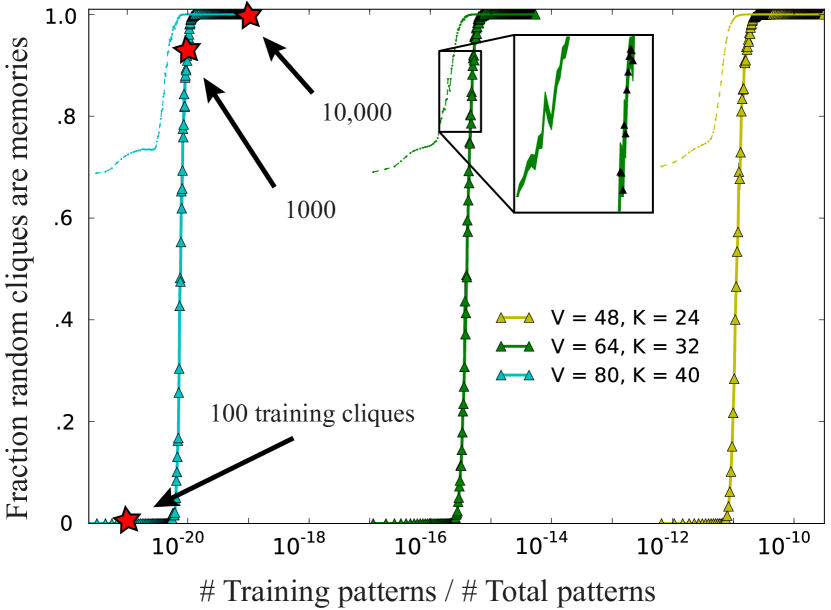
Our first result is that numerical minimization of probability flow over a vanishingly small critical number of training cliques determines linear threshold networks with exponential memory. We fit all-to-all connected networks on neurons (; ) with increasing numbers of randomly generated -cliques as training data by minimizing (4) using the limited-memory Broyden–Fletcher–Goldfarb–Shanno (L-BFGS) algorithm nocedal1980 . In Fig. 2, we plot the percentage of 1000 random new -cliques that are memories in these networks after training as a function of the ratio of training set size to total number of -cliques. Each triangle in the figure represents the average of this fraction over 50 networks, each given the same number of randomly generated (but different) training data. The finding is that a critical amount of training data gives storage of all -cliques. Moreover, this count is significantly smaller than the total number of patterns to be learned.
In Fig. 3a, we display a portion of the weight matrix with minimum probability flow representing a network (4,994,380 weight and threshold parameters) given (1e-21% of all -cliques), (1e-20%), or (1e-19%) randomly generated -cliques as training data; these are the three special red points marked in Fig. 2. In Fig. 3b, we plot histograms of the network parameters at these three training set sizes and find that the weights and thresholds become highly peaked and symmetric about three quantities. Below, we shall analytically minimize the flow objective to obtain critical symmetric parameters.
Next, we derive a biologically plausible learning rule for adapting these network parameters. Given a training pattern , the minimum probability flow (MPF) learning rule moves weights and thresholds in the direction of steepest descent of the probability flow objective function (4) evaluated at . Specifically, for the rule takes the form:
| (5) |
After learning, the weights between neurons and are symmetrized to: , which preserves the energy function and guarantees that dynamics terminates in memories. As update directions (5) descend the gradient of an infinitely differentiable convex function, learning rules based on them have good convergence rates hazan2007logarithmic . Moreover, when neurons and are both active in (5), weights increase, while when they are different they decrease, consistent with Hebb’s postulate hebb49 , a basic hypothesis about neural synaptic plasticity. In fact, approximating the exponential function with unity in (5) gives a variant of classical OPR learning. Adaptation (5) is also local in that updating weights between 2 neurons only requires their current state/threshold and feedforward input from nearby active neurons.
We now analytically minimize probability flow to determine explicit networks achieving robust exponential storage. To simplify matters, we first observe by a symmetrizing argument (see Supplementary Material) that there is a network storing all -cliques if and only if there is one with constant threshold and satisfying for each pair , ether (whenever and share one vertex) or (when and are disjoint). Weight matrices approximating this symmetry can be seen in Fig. 3a. In this case, the energy of a graph with edges is the following linear function of :
| (6) |
in which and are the number of edge pairs in the graph with exactly one or zero shared vertices, respectively.
Consider the minimization of (4) over a training set consisting of all -cliques on vertices (this simplifies the mathematics), restricting networks to our -parameter family . When , these networks are sparsely-connected, having a vanishing number of connections between neurons relative to total population size. Using single variable calculus and formula (6), it can be shown that for any fixed positive threshold , the minimum value of (4) is achieved uniquely at the parameter setting , where
| (7) |
This elementary calculation gives our first main theoretical contribution.
Theorem 1. McCulloch-Pitts networks minimizing probability flow can achieve robust exponential memory.
We prove Theorem 1 using the following large deviation theory argument; this approach also allows us to design networks achieving Shannon’s bound for low-density error-correcting codes. Fix (or ) and consider a -corrupted clique. Using Bernstein’s concentration inequality for sums of bounded random variables bernstein1924 , it can be shown that an edge in the clique has neighboring edges at least, on average, with standard deviation of order (see Supplemental Material). This gives the fixed-point requirement from (2):
On the other hand, a non-clique edge sharing a vertex with the clique has neighbors at most, on average, with standard deviation of order . Therefore, for a -clique to be a memory, this forces again from (2):
and any other edges will disappear when this holds. (Here, we use “little-o” notation .)
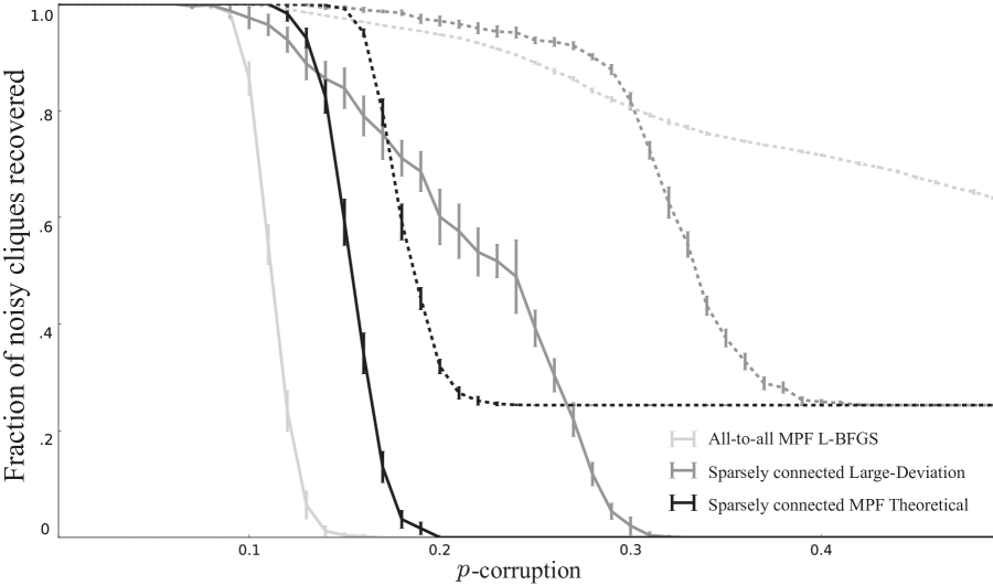
It follows that the optimal setting (7) for minimizing probability flow gives robust storage (with a single parallel dynamics update) of all -cliques for . This proves Theorem 1. It is possible to do better than robustness index by setting , which satisfies the above fixed-point requirements with probability approaching 1 for any fixed and increasing . We have thus also demonstrated:
Theorem 2. There is a family of Hopfield networks on neurons that robustly store memories with robustness index .
In Fig. 4, we show robust storage of the () -cliques in graphs on vertices using three parameter specializations designed here.
Discussion. The biologically-inspired networks introduced in this work constitute a new nonlinear error-correcting scheme that is simple to implement, parallelizable, and achieves the Shannon bound Shan48a for low-density codes over a binary symmetric channel (). There have been several other approaches to optimal error-correcting codes derived from a statistical physics perspective; for a comprehensive account, we refer the reader to vicente2002low . See also gripon2011sparse ; kumar2011exponential ; karbasi2013iterative ; curto2013combinatorial for related recent work on neural network architectures with large memory.
Although we have focused on minimizing probability flow to learn parameters in our discrete neural networks, several other strategies exist. For instance, one could maximize the (Bayesian) likelihood of cliques given network parameters, though any strategy involving a partition function over graphs will run into challenging algorithmic complexity issues jerrum1993polynomial . Contrastive divergence ackley1985learning is another popular method to estimate parameters in discrete maximum entropy models. While this approach avoids the partition function, it requires a nontrivial sampling procedure that precludes exact determination of optimal parameters.
In addition to classical coding theory and memory modeling in neuroscience, our networks also apply to a basic question in computational graph theory called the “Hidden clique problem” alon1998finding . The essential goal of this task is to find a clique that has been hidden in a graph by adding and removing edges at random. Phrased in this language, we have discovered discrete recurrent neural networks that learn to use their cooperative McCulloch-Pitts dynamics to solve hidden clique problems efficiently. For example, in Fig. 1b we show the adjacency matrices of three corrupted -cliques on vertices returning to their original configuration by one iteration of the network dynamics through all neurons.
Acknowledgements. We thank Kilian Koepsell and Sarah Marzen for helpful comments that enhanced the quality of this work. Support was provided, in part, by NSF grants IIS-0917342, IIS-1219199, IIS-1219212 (CH) and DARPA Deep Learning Program FA8650-10-C-7020 (NT). *Hillar and *Tran are listed alphabetically and contributed equally.
References
- (1) J. Hopfield, Proc. Nat. Acad. Sci. U.S.A. 79, 2554 (1982)
- (2) W. McCulloch and W. Pitts, Bull. Math. Bio. 5, 115 (1943)
- (3) J. Hopfield and D. Tank, Science 233, 625 (1986)
- (4) J. Hopfield and D. Tank, Biological cybernetics 52, 141 (1985)
- (5) C. Koch, J. Marroquin, and A. Yuille, Proc. Nat. Acad. Sci. U.S.A. 83, 4263 (1986)
- (6) R. McEliece, E. Posner, E. Rodemich, and S. Venkatesh, IEEE Trans. Info. Thry. 33, 461 (1987)
- (7) S.-I. Amari, Neural Networks 2, 451 (1989)
- (8) J. Sohl-Dickstein, P. Battaglino, and M. DeWeese, Phys. Rev. Lett. 107, 220601 (2011)
- (9) C. Shannon, Bell Sys. Tech. J. 27, 379 (1948)
- (10) N. Alon, M. Krivelevich, and B. Sudakov, Random Structures and Algorithms 13, 457 (1998)
- (11) L. Pastur and A. Figotin, Sov. J. Low Temp. Phys 3, 378 (1977)
- (12) S. Edwards and P. Anderson, J. Phys. F: Met. Phys. 5, 965 (1975)
- (13) M. Talagrand, Spin Glasses: A Challenge for Mathematicians, Vol. 46 (Springer, 2003)
- (14) D. Hebb, The Organization of Behavior (Wiley, New York, 1949)
- (15) T. Cover, IEEE Trans. Comput., 326(1965)
- (16) F. Tanaka and S. Edwards, J. Phys. F: Met. Phys. 10, 2769 (1980)
- (17) J. Platt and J. Hopfield, in Neural Networks for Computing, Vol. 151 (AIP Publishing, 1986) pp. 364–369
- (18) E. Ising, Z. Phys. 31, 253 (1925)
- (19) D. Ackley, G. Hinton, and T. Sejnowski, Cognit. Sci. 9, 147 (1985)
- (20) F. Rosenblatt, Principles of Neurodynamics: Perceptrons and the Theory of Brain Mechanisms (Spartan Books, Washington, D.C., 1961)
- (21) C. Hillar, J. Sohl-Dickstein, and K. Koepsell, in 4th Neural Information Processing Systems (NIPS) workshop on Discrete Optimization in Machine Learning (DISCML) (2012)
- (22) J. Nocedal, Math. Comp. 35, 773 (1980)
- (23) E. Hazan, A. Agarwal, and S. Kale, Machine Learning 69, 169 (2007)
- (24) S. Bernstein, Ann. Sci. Inst. Sav. Ukraine, Sect. Math 1, 38 (1924)
- (25) R. Vicente, D. Saad, and Y. Kabashima, Advances in Imaging and Electron Physics 125, 232 (2002)
- (26) V. Gripon and C. Berrou, IEEE Trans. Neural Netw. 22, 1087 (2011)
- (27) K. Kumar, A. Salavati, and A. Shokrollahi, in Information Theory Workshop (ITW), IEEE (2011) pp. 80–84
- (28) A. Karbasi, A. H. Salavati, and A. Shokrollahi, in Proceedings of The 30th International Conference on Machine Learning (2013) pp. 445–453
- (29) C. Curto, V. Itskov, K. Morrison, Z. Roth, and J. Walker, Neural Comput. 25, 1891 (2013)
- (30) M. Jerrum and A. Sinclair, SIAM Journal on Computing 22, 1087 (1993)
a) 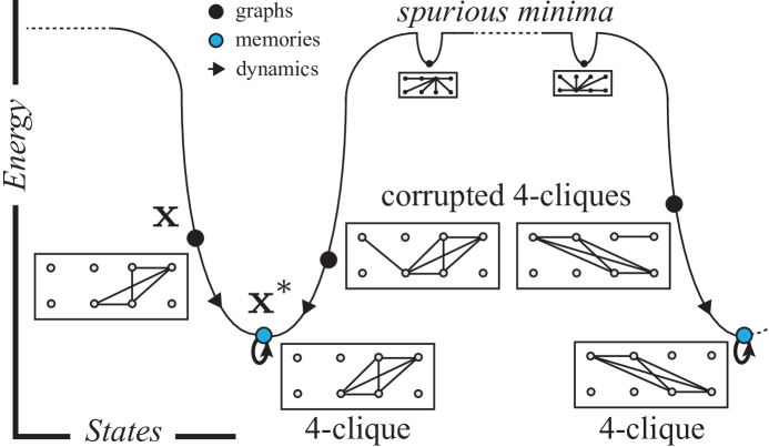
b) 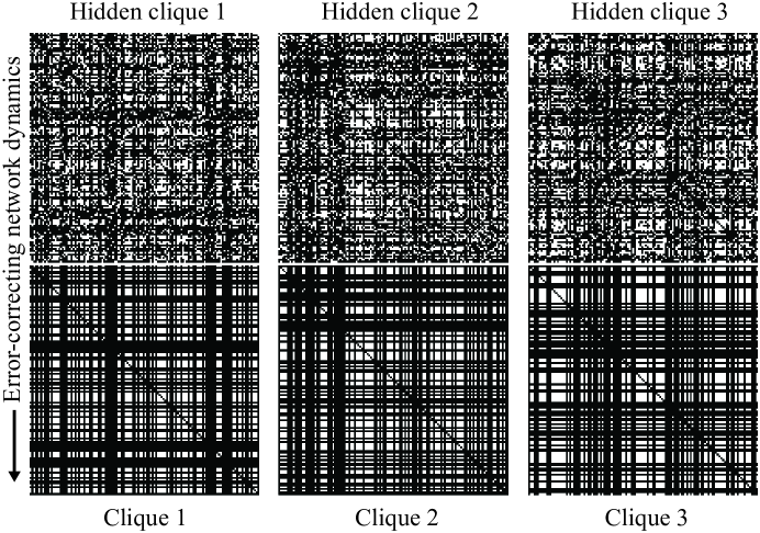
a)  b)
b) 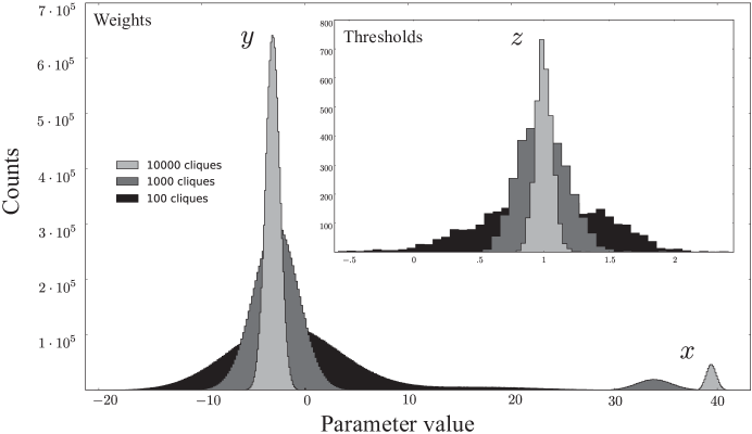
Supplementary Info
I Symmetric -parameter networks
The first step of our construction is to exploit symmetry in the following set of linear inequalities:
| (8) |
where runs over -cliques and over vectors differing from by a single bit flip. The space of solutions to (8) is the convex polyhedral cone of networks having each clique as a strict local minimum of the energy function, and thus a fixed-point of the dynamics.
The permutations of the vertices act on a network by permuting the rows/columns of the weight matrix () and thresholds (), and this action on a network satisfying property (8) preserves that property. Consider the average of a network over the group : , , and note that if satisfies (8) then so does the highly symmetric object . To characterize , observe that and .
These strong symmetries imply there are such that and for each pair of all possible edges:
where is the number of vertices that and share.
Our next demonstration is an exact setting for weights in these Hopfield networks.
II Exponential storage
For an integer , we say that state is -stable if it is an attractor for all states with Hamming distance at most from . Thus, if a state is -stably stored, the network is guaranteed to converge to when exposed to any corrupted version not more than bit flips away.
For positive integers and , is there a Hopfield network on nodes storing all -cliques -stably? We necessarily have , since is greater than or equal to the Hamming distance between two -cliques that share a -subclique. In fact, for any , this upper bound is achievable by a sparsely-connected three-parameter network.
Proposition 1. There exists a family of three-parameter Hopfield networks with , storing all -cliques as -stable states.
The proof relies on the following lemma, which gives the precise condition for the three-parameter Hopfield network to store -cliques as -stable states for fixed .
Lemma 1. Fix and . The Hopfield network stores all -cliques as -stable states if and only if the parameters satisfy
where
Furthermore, a pattern within Hamming distance of a -clique converges after one iteration of dynamics.
Proof: For fixed and -clique , there are possible patterns within Hamming distance of . Each of these patterns defines a pair of linear inequalities on the parameters . However, only the inequalities from the following two extreme cases are active constraints. All the other inequalities are convex combinations of these.
-
1.
edges in the clique with a common node are removed.
-
2.
edges are added to a node not in the clique.
In the first case, there are two types of edges at risk of being mislabeled. The first are those of the form for all nodes in the clique. Such an edge has neighbors and non-neighbors. Thus, each such edge will correctly be labeled as after one network update if and only if , , and satisfy
| (9) |
The other type are those of the form for all nodes in the clique, and not in the clique. Assuming , such an edge has at most neighbors and non-neighbors. Thus, each such edge will be correctly labeled as if and only if
| (10) |
Rearranging equations (9) and (10) yield the first two rows of the matrix in the lemma. A similar argument applies for the second case, giving the last two inequalities.
From the derivation, it follows that if a pattern is within Hamming distance of a -clique, then all spurious edges are immediately deleted by case 1, all missing edges are immediately added by case 2, and thus the clique is recovered in precisely one iteration of the network dynamics.
Proof of Proposition 1: The matrix inequalities in Lemma 1 define a cone in , and the cases or correspond to two separate components of this cone. For the proof of Theorem 1 in the main article, we shall use the cone with . We further assume to achieve a sparsely-connected matrix . In this case, the second and fourth constraints are dominated by the first and third. Thus, we need that solves:
There exists such a solution if and only if
| (11) |
The above equation is feasible if and only if .
III Proofs of Theorems 1, 2
Fix and . We now tune such that asymptotically the -robustness of our set of Hopfield networks storing -cliques tends to as . By symmetry, it is sufficient to prove robustness for one fixed -clique , say, the one with vertices . For , let be the -corruption of . For each node , let denote the number of edges from to other clique and non-clique nodes, respectively. With an abuse of notation, we write to mean a vertex in the clique, that is, . We need the following inequality originally due to Bernstein [24].
Lemma 2 (Bernstein’s inequality). Let be independent Bernoulli random variables taking values and each with probability . For any , the following holds:
The following fact is a fairly direct consequence of Lemma 2.
Lemma 3. Let be an symmetric matrix with zero diagonal, . For each , let be the -th row sum. Let , and . Then for any constant , as , we have:
and
In particular, .
Proof: Fix . As a direct corollary of Bernstein’s inequality, for each and for any , we have
It follows that
and thus from a union bound with , we have
Since this last bound converges to with , we have proved the claim for . Since is symmetric about , a similar inequality holds for .
Corollary 1. Let , , , , and . Then , , , , and are all of order as almost surely.
Proofs of Theorem 1, 2 (robustness): Let be the number of neighbors of edge . For each in the clique:
To guarantee that all edges in the clique are labeled 1 after one dynamics update, we need ; that is,
| (12) |
If is an edge with exactly one clique vertex, then
To guarantee that for all such edges after one iteration of the dynamics, we need ; that is,
| (13) |
In particular, if for some small , then taking would guarantee that for large , both equations (12) and (13) are simultaneous satisfied. In this case, , and thus the family of two-parameter Hopfield networks with , , has robustness index .
IV Clique range storage
In this section, we give precise conditions for the existence of a Hopfield network on nodes that stores all -cliques for in an interval , . We do not address the issue of robustness as the qualitative trade-off is clear: the more memories the network is required to store, the less robust it is. The trade-off can be analyzed by large deviation principles as in Theorem 2.
Theorem 3. Fix such that . For , there exists a Hopfield network on nodes which stores all -cliques in the range if and only if solves the implicit equation , where
Proof of Theorem 3: Fix and in Lemma 1. (We do not impose the constraint ). Then the cone defined by the inequalities in Lemma 1 is in bijection with the polyhedron cut out by inequalities:
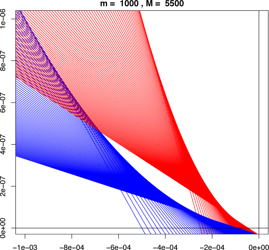
Let be the line , and be the line . By symmetry, there exists a Hopfield network which stores all -cliques in the range if and only if . For a point , write for its -coordinate. Note that for , the points lie on the following curve implicitly parametrized by :
When the polytope is nonempty, its vertices are the following points: , for , and the points . This defines a nonempty convex polytope if and only if
Direct computation gives the formulae for in Theorem 3. See Fig 6 for a visualization of the constraints of the feasible region.
Fixing the number of nodes and optimizing the range in Theorem 3, we obtain the following result.
Theorem 4. For large , there is a Hopfield network on nodes that stores all cliques of size as memories, where is in the range:
for constants , . Moreover, this is the largest possible range of for any Hopfield network.
Proof of Theorem 4: From Theorem 3, for large and , we have the approximations , . Hence when . Asymptotically for large , the most cliques are stored when and contains . Consider so that , and thus . Next, set and so that storing the most cliques becomes the problem of maximizing over admissible the quantity:
One can now check that gives the best value, producing the range in the statement of the theorem.
Next, note that is the fraction of -cliques in all cliques on vertices, which is also the probability of a variable equaling . For large , approximating this variable with a normal distribution and then using Mill’s ratio to bound its tail c.d.f. , we see that the proportion of cliques storable tends to
for some constant .
V Hopfield-Platt networks
We prove the claim in the main text that the Hopfield-Platt network will not robustly store derangements (permutations without fixed-points). For large , the fraction of permutations that are derangements is known to be . Fix a derangement on , represented as a binary vector in for . For each ordered pair , , , we construct a pattern that differs from by exactly two bit flips:
-
1.
Add the edge .
-
2.
Remove the edge .
There are such pairs , and thus different patterns . For each such pattern, we flip two more bits to obtain a new permutation as follows:
-
1.
Remove the edge .
-
2.
Add the edge .
It is easy to see that is a permutation on letters with exactly two cycles determined by . Call the set of edges modified the critical edges of the pair . Note that are all distinct and have disjoint critical edges.
Each is exactly two bit flips away from and , both permutations on letters. Starting from , there is no binary Hopfield network storing all permutations that always correctly recovers the original state. In other words, for a binary Hopfield network, is an indistinguishable realization of a corrupted version of and .
We now prove that for each derangement , with probability at least , its -corruption is indistinguishable from the -corruption of some other permutation. This implies the statement in the main text.
For each pair as above, recall that and are two random variables in obtained by flipping each edge of (resp. ) independently with probability . We construct a coupling between them as follows: define the random variable via
-
•
For each non-critical edge, flip this edge on and with the same .
-
•
For each critical edge, flip them on and with independent .
Then have the same distribution, and and only differ in distribution on the four critical edges. Their marginal distributions on these four edges are two discrete variables on states, with total variation distance . Thus, there exists a random variable such that , and
In other words, given a realization of , with probability , this is equal to a realization from the distribution of , and therefore no binary Hopfield network storing both and can correctly recover the original state from such an input. An indistinguishable realization occurs when two of the four critical edges are flipped in a certain combination. For fixed , there are such where the critical edges are disjoint. Thus, the probability of being an indistinguishable realization from a realization of one of the is at least
completing the proof of the claim.
VI Examples of clique storage robustness
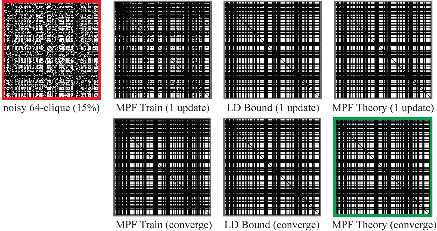
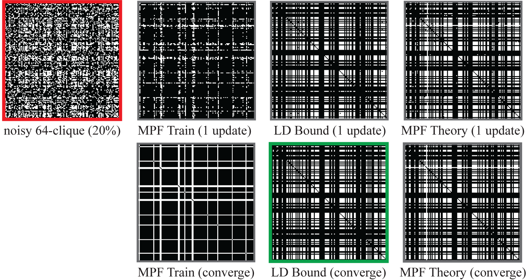
Finally, in Fig 5 below we present examples of robust storage of cliques for the networks in Fig. 4 of the main text.
a 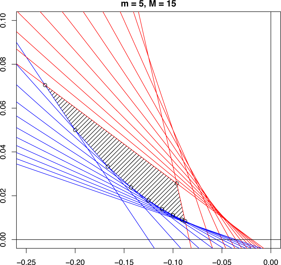
b 