Optimal Reduction of Multivariate
Dirac Mixture Densities

Abstract

This paper is concerned with the optimal approximation of a given multivariate Dirac mixture, i.e., a density comprising weighted Dirac distributions on a continuous domain, by an equally weighted Dirac mixture with a reduced number of components. The parameters of the approximating density are calculated by minimizing a smooth global distance measure, a generalization of the well-known Cramér-von Mises Distance to the multivariate case. This generalization is achieved by defining an alternative to the classical cumulative distribution, the Localized Cumulative Distribution (LCD), as a characterization of discrete random quantities (on continuous domains), which is unique and symmetric also in the multivariate case. The resulting approximation method provides the basis for various efficient nonlinear state and parameter estimation methods.

1 Introduction

1.1 Motivation

We consider point sets ${\cal P}_{x}=\{\underline{x}_{1},\underline{x}_{2},\ldots,\underline{x}_{L}\}$ where the points $\underline{x}_{i}$, $i=1,\ldots,L$ are arbitrarily placed in $\mathbb{R}^{N}$, i.e., $\underline{x}_{i}\in\mathbb{R}^{N}$, $i=1,\ldots,L$. The points can be of arbitrary origin, e.g., be samples from a Probability density function, and can be interpreted as being equally weighted or be equipped with weights. When they are weighted, we assume the weights $w_{i}$ associated with point $\underline{x}_{i}$ for $i=1,\ldots,L$ to be positive and sum up to one.

The point sets are interpreted as discrete Probability density functions over a continuous domain, where the individual points correspond to locations of Dirac distributions with associated weights. The point set will be called a Dirac mixture density. Dirac mixture densities are a popular representation of densities in stochastic nonlinear filters such as particle filters. They characterize random vectors in a similar way as sets of sample points by having a large number of components with large weights in regions of high density and a small number of components with small weights in regions of low density. Hence, approximating one Dirac mixture density by another one while maintaining the information content is equivalent to maintaining its probability mass distribution.

Reducing the size of a point set while maintaining its information content as much as possible is a fundamental problem occurring in many flavors in different contexts. One example is a large number of noisy samples from an underlying unknown probability density function. The goal is to represent the underlying density by a reduced set of well-placed Dirac components while removing the noise. The need for reduction also occurs, when the given point set is too complex for further processing. During the recursive processing of Dirac mixtures, for example in a nonlinear filter, the number of components often explodes. A typical example is the propagation of Dirac mixture densities through a discrete-time dynamic system, which requires a kind of generalized convolution with the noise density. After one processing step, the number of components is given by the product of the given number of components times the number of components used for representing the noise density, which results in an exponential increase with the number of processing steps. Hence, the goal is to keep the number of components at a manageable level by performing regular reductions.

1.2 Related Work

We will now take a look at different methods that have been devised in the general context of reduction of point sets or densities.

Random Selection

The most common technique for reducing the number of components of a given Dirac mixture density is the random selection of certain components. It is commonly used in the prediction step of Particle Filters, where each prior sample is perturbed with a single sample from the noise distribution before propagation thorough the system model. The perturbation can be viewed as generating the noise samples at once with a subsequent random selection from the Cartesian product of prior samples and noise samples.

Intermediate Continuous Densities

Another common technique is to replace the given Dirac mixture by a suitable continuous density in a first step. In a second step, the desired number of samples is drawn from the continuous density. With this technique, it is also possible to increase the number of components as required. However, the first step is equivalent to density estimation from samples, which is by itself a complicated task and an active research topic. Furthermore, this reduction technique introduces undesired side information via the choice of the continuous smoothing density.

Clustering or Vector Quantization Methods

Clustering or vector quantization methods also aim at representing a point set by a smaller set of representatives. For optimization purposes, a distortion measure is typically used, which sums up the (generalized) distances between the points and their representatives. Minimizing the distortion measure results in two conditions: 1. Points are associated to their closest representative. 2. The representative is calculated as the average of all its associated points. As no closed-form solution for performing the minimization of the distortion measure exist, robust iterative procedures have been devised starting with Lloyd’s algorithm proposed in 1957 and published later in lloyd_least_1982 , first called k-means algorithm in macqueen_methods_1967 , and its extension in the form of the Linde-Buzo-Gray-algorithm linde_algorithm_1980 . Obviously, the representatives fulfilling the above two conditions do not necessarily maintain the form of the density, which will also be shown by some examples in Sec. 7 of this paper. An additional problem of clustering or vector quantization methods is that the iterative minimization procedures typically get stuck in local minima. Intuitively, the resulting samples are only influenced by samples in the corresponding part of the Voronoi diagram, while the proposed method is based upon a global distance measure.

Reapproximating Continuous Mixtures with Continuous Mixtures

As Dirac mixture reduction is a special case of general mixture reduction techniques. As these techniques are usually focused on continuous densities such as Gaussian mixtures, e.g., see crouse_look_2011 , it is worthwhile to discuss the differences. First, when continuous mixtures are re-approximated with continuous mixtures, the densities or parts of the densities can be directly compared in terms of the integral squared difference williams_cost-function-based_2003 or the Kullback-Leibler divergence runnalls_kullback-leibler_2007 . Directly comparing densities with an integral measure is not possible when at least one of the densities is a Dirac mixture density MFI08_Hanebeck-LCD . Instead, cumulative distributions can be used in the scalar case or appropriate generalizations for the multivariate case MFI08_Hanebeck-LCD . Second, for continuous mixtures two or more critical components can be merged in order to locally reduce the number of components west_approximating_1993 , where different criteria for identifying components are possible such as small weights. These components are then replaced by a new component with appropriate parameters, e.g., maintaining mean and covariance. Locally replacing components is not straightforward for Dirac mixture densitys as it is i) difficult to identify potential merging candidates and ii) a single replacement component does not capture the extent covered by the original components. Hence, a replacement of several Dirac components by a smaller set of Dirac components with a cardinality larger than one would be in order.

Reapproximating Continuous Mixtures with Discrete Mixtures

The reduction problem can be viewed as approximating a given (potentially continuous) density with a Dirac mixture density. Several options are available for performing this approximation. Moment-based approximations have been proposed in the context of Gaussian densities and Linear Regression Kalman Filters (LRKFs), see lefebvre_linear_2005 . Examples are the Unscented Kalman Filter (UKF) in julier_new_2000 and its scaled version in julier_scaled_2002 , its higher-order generalization in tenne_higher_2003 , and a generalization to an arbitrary number of deterministic samples placed along the coordinate axes introduced in IFAC08_Huber . For Circular probability density functions, a first approach to Dirac mixture approximation in the vein of the UKF is introduced in ACC13_Kurz for the Von Mises distribution and the Wrapped Normal distribution. Three components are systematically placed based on matching the first Circular moment. This Dirac mixture approximation of continuous Circular probability density functions has already been applied to sensor scheduling based on bearings-only measurements Fusion13_Gilitschenski . In IPIN13_Kurz , the results are used to perform recursive circular filtering for tracking an object constrained to an arbitrary one-dimensional manifold. For the case that only a finite set of moments of a random vector is given and the underlying density is unknown, an algorithm is proposed in arXiv14_Hanebeck for calculating multivariate Dirac mixture densities with an arbitrary number of arbitrarily placed components maintaining these moments while providing a homogeneous coverage of the state space. This method could also be used for the reduction problem by calculating the moments of the given point set. Methods that are based on distance measures between the given density and its Dirac mixture approximation have been proposed for the case of scalar continuous densities in CDC06_Schrempf-DiracMixt ; MFI06_Schrempf-CramerMises . They are based on distance measures between cumulative distribution functions. These distance-based approximation methods are generalized to the multi-dimensional case by defining an alternative to the classical cumulative distribution, the Localized Cumulative Distribution (LCD) MFI08_Hanebeck-LCD , which is unique and symmetric. Based on the LCD, multi-dimensional Gaussian densities are approximated by Dirac mixture densities in CDC09_HanebeckHuber . A more efficient method for the case of standard Normal distributions with a subsequent transformation is given in ACC13_Gilitschenski .

The LCD-based methods will be extended to the reduction of Dirac mixture densities in this paper. A variant of the reduction problem, the optimal approximation of the Cartesian product of marginal Dirac mixture densities is considered in ACC10_Eberhardt and a solution is proposed that does not require the explicit calculation of all combinations of marginal components.

1.3 Key Ideas and Results of the Paper

The key idea of this paper is the systematic reapproximation of Dirac mixture densities by minimization of a novel distance measure. The distance measure compares the probability masses of both densities under certain kernels for all possible kernel locations and widths, which allows the use of integral measures for the mass functions. This approximation method is similar to the approximation of multivariate Gaussian densities by Dirac mixtures in CDC09_HanebeckHuber . However, calculating the distance measure between multivariate Gaussians and Dirac mixture densities in CDC09_HanebeckHuber requires a one-dimensional numerical approximation, while the distance measure for comparing Dirac mixture densities with Dirac mixture densities proposed in this paper is given in closed from.

The resulting distance measure is smooth and does not suffer from local minima, so that standard optimization methods can be used for calculating the desired Dirac mixture approximation. As no randomness is involved, the optimization results are completely deterministic and reproducible, which is in contrast to random selection procedures and most clustering methods.

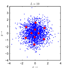
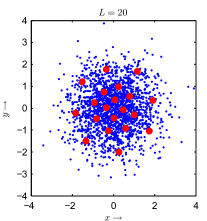
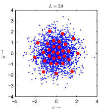
The results for approximating $2000$ samples from a standard Normal distribution by a Dirac mixture approximation with $L=10$, $L=20$, and $L=30$ components are shown in Fig. 1.

Figure 1: Dirac mixture approximation of $2000$ samples from a standard Normal distribution with $L=10$, $L=20$, and $L=30$. Blue: Random samples representing the standard Normal distribution. Red: Reduced point set.

1.4 Organization of the Paper

In the next section, a rigorous formulation of the considered approximation problem is given. For comparing Dirac mixture densities, an alternative to the classical cumulative distribution, the so called Localized Cumulative Distribution (LCD) is introduced in Sec. 3. Based on this LCD, a generalization of the Cramér-von Mises Distance, which is the squared integral difference between the LCD of the given density and the LCD of the approximate density is given in Sec. 4. This new distance measure is used for analysis purposes, i.e., for comparing the approximate Dirac mixture to the given one. The synthesis problem, i.e., determining the parameters of the approximate Dirac mixture in such a way that it is as close as possible to the given Dirac mixture according to the new distance measure is the topic of Sec. 5. Minimization is performed with a quasi-Newton method. The required gradient is derived in Appendix A, which also gives necessary conditions for a minimum distance in the form of a set of nonlinear equations. The complexity of both calculating the distance measure and its gradient in practical situations is derived in Sec. 6. Examples of using the new reduction method on specific point sets are given in Sec. 7. The new approach is discussed in Sec. 8 and an outlook to future work is given.

2 Problem Formulation

We consider an $N$–dimensional Dirac mixture density with $M$ components given by

$$\tilde{f}(\underline{x})=\sum_{i=1}^{M}w_{i}^{y}\,\delta(\underline{x}-\underline{y}_{i})\enspace,$$

with positive weights $w_{i}^{y}>0$, i.e., $w_{i}^{y}>0$, for $i=1,\ldots,M$, that sum up to one and $M$ locations $\underline{y}_{i}=\begin{bmatrix}y_{i}^{(1)},y_{i}^{(2)},\ldots,y_{i}^{(N)}\end{bmatrix}^{T}$ for $i=1,\ldots,M$. This density is approximated by another $N$–dimensional Dirac mixture density with $L$ components given by

$$f(\underline{x})=\sum_{i=1}^{L}w_{i}^{x}\,\delta(\underline{x}-\underline{x}_{i})\enspace,$$ (1)

with positive weights $w_{i}^{x}$, i.e., $w_{i}^{x}>0$, for $i=1,\ldots,L$, that sum up to one and $L$ locations $\underline{x}_{i}=\begin{bmatrix}x_{i}^{(1)},x_{i}^{(2)},\ldots,x_{i}^{(N)}\end{bmatrix}^{T}$ for $i=1,\ldots,L$, where we typically assume $L\leq M$.

The goal is to select the location parameters $\underline{x}_{i}$, $i=1,\ldots,L$ of the approximating density $f(\underline{x})$ in such a way that a distance measure $D$ between the true density $\tilde{f}(\underline{x})$ and its approximation $f(\underline{x})$ is systematically minimized. The weights $w_{i}^{x}$, $i=1,\ldots,L$ are assumed to be given and are typically set to be equal. An extension to given unequal weights or to even optimizing the weights of $f(\underline{x})$ is a simple extension that is not pursued in this paper.

The true Dirac mixture density might already have equally weighted components, so that the information is solely stored in the component locations. In this case, the goal of the approximation is a pure reduction of the number of components. On the other hand, the components of the true Dirac mixture density might have different weights. This could be the result of, e.g., weighting a prior Dirac mixture density by a likelihood function in a Bayesian filtering setup. In that case, the approximation replaces an arbitrarily weighted Dirac mixture density by an equally weighted one. In the latter case, an equal number of components, i.e., $L=M$, can be useful.

3 Localized Cumulative Distribution

For the systematic reduction of the number of components of a given Dirac mixture density, a distance measure for comparing the original density and its approximation is required. However, Dirac mixture densities cannot be directly compared as they typically do not even share a common support. Typically, their corresponding cumulative distributions are used for comparison purposes, as is the case in certain statistical tests such as the Kolmogov-Smirnov test (press_numerical_1992, , p. 623). However, it has been shown in MFI08_Hanebeck-LCD that although the cumulative distribution is well suited for comparing scalar densities, it exhibits several problems in higher-dimensional spaces: It is non-unique and non-symmetric. In addition, integral measures for comparing two cumulative distributions do not converge over infinite integration domains when the underlying Dirac mixture densities differ.

As an alternative transformation of densities, the Localized Cumulative Distribution (LCD) introduced in MFI08_Hanebeck-LCD is employed here in a generalized form. An LCD is an integral measure proportional to the mass concentrated in a region with a size parametrized by a vector $\underline{b}$ around test points $\underline{m}$. These regions are defined by kernels $K(\underline{x}-\underline{m},\underline{b})$ centered around $\underline{m}$ with size $\underline{b}$.

Definition 3.1.

Let $\underline{\boldsymbol{x}}$ be a random vector with $\underline{\boldsymbol{x}}\in\mathbb{R}^{N}$, which is characterized by an $N$–dimensional probability density function $f:\mathbb{R}^{N}\!\!\rightarrow\!\!\mathbb{R}_{+}$. The corresponding Localized Cumulative Distribution (LCD) is defined as

$$F(\underline{m},\underline{b})=\int_{\mathbb{R}^{N}}f(\underline{x})\,K(\underline{x}-\underline{m},\underline{b})\,d\underline{x}$$

with $\underline{b}\in\mathbb{R}_{+}^{N}$ and $F(.,.):\Omega\rightarrow[0,1],\Omega\subset\mathbb{R}^{N}\times\mathbb{R}_{+}^{N}$.

Definition 3.2.

As a shorthand notation, we will denote the relation between the density $f(\underline{x})$ and its LCD $F(\underline{x},\underline{b})$ by

$$f(\underline{x})\;\laplace\;F(\underline{m},\underline{b})\enspace.$$

In this paper, we focus attention on separable kernels of the type

$$K(\underline{x}-\underline{m},\underline{b})=\prod_{k=1}^{N}K(x^{(k)}-m^{(k)},b^{(k)})\enspace.$$

Furthermore, we consider kernels with equal width in every dimension, i.e., $b_{i}=b$ for $i=1,\ldots,N$, which gives

$$K(\underline{x}-\underline{m},b)=\prod_{i=k}^{N}K(x^{(k)}-m^{(k)},b)\enspace.$$

Rectangular, axis-aligned kernels as used in MFI08_Hanebeck-LCD are the obvious choice as they yield the probability mass of the considered density in a rectangular region centered around $\underline{m}$. Rectangular kernels are a good choice for analysis purposes and are used, e.g., when assessing the discrepancy of a point set from a uniform distribution.

However, for synthesizing a suitable approximation for a given (nonuniform) Dirac mixture with a smaller number of components, smooth kernels lead to simpler optimization problems. Here, we consider kernels of Gaussian type according to

$$K(\underline{x}-\underline{m},b)=\prod_{k=1}^{N}\exp\left(-\frac{1}{2}\frac{\left(x^{(k)}-m^{(k)}\right)^{2}}{b^{2}}\right)\enspace.$$

Based on a Gaussian kernel, an N-dimensional Dirac component $\delta(\underline{x}-\hat{\underline{x}})$ at location $\hat{\underline{x}}$ corresponds to its LCD $\Delta(\underline{m},b)$

$$\delta(\underline{x}-\hat{\underline{x}})\;\laplace\;\Delta(\underline{m},b)$$

with

$$\begin{split}\Delta(\underline{m},b)&=\int_{\mathbb{R}^{N}}\delta(\underline{x}-\hat{\underline{x}})\,K(\underline{x}-\underline{m},\underline{b})\,d\underline{x}\\ &=\prod_{k=1}^{N}\exp\left(-\frac{1}{2}\frac{\left(\hat{x}^{(k)}-m^{(k)}\right)^{2}}{b^{2}}\right)\enspace.\end{split}$$

With this LCD of a single Dirac component, the LCD of the Dirac mixture in (1) is given by

$$F(\underline{m},b)=\sum_{i=1}^{L}w_{i}^{x}\,\prod_{k=1}^{N}\exp\left(-\frac{1}{2}\frac{\left(x_{i}^{(k)}-m^{(k)}\right)^{2}}{b^{2}}\right)\enspace.$$

A similar result holds for the original Dirac mixture $\tilde{f}(\underline{x})$.

4 A Modified Cramér-von Mises Distance

The Localized Cumulative Distribution (LCD) defined previously can now be used to derive a modified version of the Cramér-von Mises Distance suitable for comparing Dirac Mixtures. This new distance is defined as the integral of the square of the difference between the LCD of the true density $\tilde{f}(\underline{x})$ and the LCD of its approximation $f(\underline{x})$.

Definition 4.1 (Modified Cramér-von Mises Distance).

The distance $D$ between two densities $\tilde{f}(\underline{x}):\mathbb{R}^{N}\rightarrow\mathbb{R}_{+}$ and $f(\underline{x}):\mathbb{R}^{N}\rightarrow\mathbb{R}_{+}$ is given in terms of their corresponding LCDs $\tilde{F}(\underline{x},b)$ and $F(\underline{x},b)$ as

$$D=\int_{\mathbb{R}_{+}}w(b)\int_{\mathbb{R}^{N}}\left(\tilde{F}(\underline{m},b)-F(\underline{m},b)\right)^{2}\,d\underline{m}\,db\enspace,$$

where $w(b):\mathbb{R}_{+}\rightarrow[0,1]$ is a suitable weighting function.

A weighting function $w(b)$ has been introduced that controls how kernels of different sizes influence the resulting distance, which provides some degrees of freedom during the design of an approximation algorithm. Alternatively, a unit weighting function could be used while modifying the kernels accordingly.

Theorem 4.1.

By inserting the LCDs

$$\tilde{F}(\underline{m},b)=\sum_{i=1}^{M}w_{i}^{y}\prod_{k=1}^{N}\exp\left(-\frac{1}{2}\frac{(y_{i}^{(k)}-m^{(k)})^{2}}{b^{2}}\right)$$

and

$$F(\underline{m},b)=\sum_{i=1}^{L}w_{i}^{x}\prod_{k=1}^{N}\exp\left(-\frac{1}{2}\frac{(x_{i}^{(k)}-m^{(k)})^{2}}{b^{2}}\right)\enspace,$$

and by using the weighting function

$$w(b)=\begin{cases}\frac{1}{b^{N-1}}&b\in[0,b_{\text{max}}]\\ 0&\text{elsewhere}\end{cases}$$

the following expressions for the distance $D$

$$\begin{split}D=\sum_{i=1}^{M}\sum_{j=1}^{M}w_{i}^{y}w_{j}^{y}&\,\gamma\left(\displaystyle\sum_{k=1}^{N}\left(y_{i}^{(k)}-y_{j}^{(k)}\right)^{2}\right)\\ -2\sum_{i=1}^{L}\sum_{j=1}^{M}w_{i}^{x}w_{j}^{y}&\,\gamma\left(\displaystyle\sum_{k=1}^{N}\left(x_{i}^{(k)}-y_{j}^{(k)}\right)^{2}\right)\\ +\sum_{i=1}^{L}\sum_{j=1}^{L}w_{i}^{x}w_{j}^{x}&\,\gamma\left(\displaystyle\sum_{k=1}^{N}\left(x_{i}^{(k)}-x_{j}^{(k)}\right)^{2}\right)\end{split}$$

with

$$\gamma(z)=\frac{\pi^{\frac{N}{2}}}{8}\left\{4\,b_{\text{max}}^{2}\,\exp\left(-\frac{1}{2}\frac{z}{2\,b_{\text{max}}^{2}}\right)+z\,\operatorname{Ei}\left(-\frac{1}{2}\frac{z}{2\,b_{\text{max}}^{2}}\right)\right\}\enspace,$$

are obtained, where $\operatorname{Ei}(z)$ denotes the exponential integral.

Proof.

For the given specific weighting function $w(b)$, the distance measure is given by

$$D=\int_{0}^{b_{\text{max}}}\frac{1}{b^{N-1}}\int_{\mathbb{R}^{N}}\left(\tilde{F}(\underline{m},b)-F(\underline{m},b)\right)^{2}\,d\underline{m}\,db\enspace.$$ (2)

Inserting the LCDs $\tilde{F}(\underline{m},b)$ and $F(\underline{m},b)$ leads to

$$\begin{split}D=\int_{0}^{b_{\text{max}}}\frac{1}{b^{N-1}}\int_{\mathbb{R}^{N}}\sum_{i=1}^{M}\sum_{j=1}^{M}w_{i}^{y}w_{j}^{y}&\prod_{k=1}^{N}\exp\left(-\frac{1}{2}\frac{(y_{i}^{(k)}-m^{(k)})^{2}}{b^{2}}\right)\\ &\prod_{k=1}^{N}\exp\left(-\frac{1}{2}\frac{(y_{j}^{(k)}-m^{(k)})^{2}}{b^{2}}\right)\\ -2\sum_{i=1}^{L}\sum_{j=1}^{M}w_{i}^{x}w_{j}^{y}&\prod_{k=1}^{N}\exp\left(-\frac{1}{2}\frac{(x_{i}^{(k)}-m^{(k)})^{2}}{b^{2}}\right)\\ &\prod_{k=1}^{N}\exp\left(-\frac{1}{2}\frac{(y_{j}^{(k)}-m^{(k)})^{2}}{b^{2}}\right)\\ +\sum_{i=1}^{L}\sum_{j=1}^{L}w_{i}^{x}w_{j}^{x}&\prod_{k=1}^{N}\exp\left(-\frac{1}{2}\frac{(x_{i}^{(k)}-m^{(k)})^{2}}{b^{2}}\right)\\ &\prod_{k=1}^{N}\exp\left(-\frac{1}{2}\frac{(x_{j}^{(k)}-m^{(k)})^{2}}{b^{2}}\right)\,d\underline{m}\,db\enspace.\end{split}$$

Exchanging integration and summation gives

$$\begin{split}D=\sum_{i=1}^{M}\sum_{j=1}^{M}w_{i}^{y}w_{j}^{y}&\int_{0}^{b_{\text{max}}}\frac{1}{b^{N-1}}\prod_{k=1}^{N}\int_{\mathbb{R}}\exp\left(-\frac{1}{2}\frac{(y_{i}^{(k)}-m^{(k)})^{2}}{b^{2}}\right)\exp\left(-\frac{1}{2}\frac{(y_{j}^{(k)}-m^{(k)})^{2}}{b^{2}}\right)dm^{(k)}\,db\\ -2\sum_{i=1}^{L}\sum_{j=1}^{M}w_{i}^{x}w_{j}^{y}&\int_{0}^{b_{\text{max}}}\frac{1}{b^{N-1}}\prod_{k=1}^{N}\int_{\mathbb{R}}\exp\left(-\frac{1}{2}\frac{(x_{i}^{(k)}-m^{(k)})^{2}}{b^{2}}\right)\exp\left(-\frac{1}{2}\frac{(y_{j}^{(k)}-m^{(k)})^{2}}{b^{2}}\right)dm^{(k)}\,db\\ +\sum_{i=1}^{L}\sum_{j=1}^{L}w_{i}^{x}w_{j}^{x}&\int_{0}^{b_{\text{max}}}\frac{1}{b^{N-1}}\prod_{k=1}^{N}\int_{\mathbb{R}}\exp\left(-\frac{1}{2}\frac{(x_{i}^{(k)}-m^{(k)})^{2}}{b^{2}}\right)\exp\left(-\frac{1}{2}\frac{(x_{j}^{(k)}-m^{(k)})^{2}}{b^{2}}\right)dm^{(k)}\,db\end{split}$$

For further simplification, the following closed-form expression for the occurring integrals

$$\int_{\mathbb{R}}\exp\left(-\frac{1}{2}\frac{(z_{i}-m)^{2}}{b^{2}}\right)\exp\left(-\frac{1}{2}\frac{(z_{j}-m)^{2}}{b^{2}}\right)dm=\sqrt{\pi}\,b\,\exp\left(-\frac{1}{2}\frac{(z_{i}-z_{j})^{2}}{2\,b^{2}}\right)\enspace,$$ (3)

is used. This gives

$$\begin{split}D=\sum_{i=1}^{M}\sum_{j=1}^{M}w_{i}^{y}w_{j}^{y}&\int_{0}^{b_{\text{max}}}b\,\pi^{\frac{N}{2}}\prod_{k=1}^{N}\exp\left(-\frac{1}{2}\frac{\left(y_{i}^{(k)}-y_{j}^{(k)}\right)^{2}}{2\,b^{2}}\right)\,db\\ -2\sum_{i=1}^{L}\sum_{j=1}^{M}w_{i}^{x}w_{j}^{y}&\int_{0}^{b_{\text{max}}}b\,\pi^{\frac{N}{2}}\prod_{k=1}^{N}\exp\left(-\frac{1}{2}\frac{\left(x_{i}^{(k)}-y_{j}^{(k)}\right)^{2}}{2\,b^{2}}\right)\,db\\ +\sum_{i=1}^{L}\sum_{j=1}^{L}w_{i}^{x}w_{j}^{x}&\int_{0}^{b_{\text{max}}}b\,\pi^{\frac{N}{2}}\prod_{k=1}^{N}\exp\left(-\frac{1}{2}\frac{\left(x_{i}^{(k)}-x_{j}^{(k)}\right)^{2}}{2\,b^{2}}\right)\,db\enspace.\end{split}$$

or

$$\begin{split}D=\sum_{i=1}^{M}\sum_{j=1}^{M}w_{i}^{y}w_{j}^{y}&\int_{0}^{b_{\text{max}}}b\,\pi^{\frac{N}{2}}\exp\left(-\frac{1}{2}\frac{\displaystyle\sum_{k=1}^{N}\left(y_{i}^{(k)}-y_{j}^{(k)}\right)^{2}}{2\,b^{2}}\right)\,db\\ -2\sum_{i=1}^{L}\sum_{j=1}^{M}w_{i}^{x}w_{j}^{y}&\int_{0}^{b_{\text{max}}}b\,\pi^{\frac{N}{2}}\exp\left(-\frac{1}{2}\frac{\displaystyle\sum_{k=1}^{N}\left(x_{i}^{(k)}-y_{j}^{(k)}\right)^{2}}{2\,b^{2}}\right)\,db\\ +\sum_{i=1}^{L}\sum_{j=1}^{L}w_{i}^{x}w_{j}^{x}&\int_{0}^{b_{\text{max}}}b\,\pi^{\frac{N}{2}}\exp\left(-\frac{1}{2}\frac{\displaystyle\sum_{k=1}^{N}\left(x_{i}^{(k)}-x_{j}^{(k)}\right)^{2}}{2\,b^{2}}\right)\,db\enspace.\end{split}$$

With

$$\int_{0}^{b_{\text{max}}}b\,\exp\left(-\frac{1}{2}\frac{z}{2\,b^{2}}\right)\,db=\frac{1}{8}\left\{4\,b_{\text{max}}^{2}\,\exp\left(-\frac{1}{2}\frac{z}{2\,b_{\text{max}}^{2}}\right)+z\,\operatorname{Ei}\left(-\frac{1}{2}\frac{z}{2\,b_{\text{max}}^{2}}\right\}\right)$$

for $z>0$, the final result is obtained. ∎

Remark 4.1.

The exponential integral $\operatorname{Ei}(z)$ is defined as

$$\operatorname{Ei}(z)=\int_{-\infty}^{z}\frac{e^{t}}{t}dt\enspace.$$

For $z>0$, $\operatorname{Ei}(z)$ is related to the incomplete gamma function $\Gamma(0,z)$ according to

$$\operatorname{Ei}(-z)=-\Gamma(0,z)\enspace.$$

Theorem 4.2.

For large $b_{\text{max}}$, the distance $D$ is described by

$$D=\frac{\pi^{\frac{N}{2}}}{8}\left(D_{\underline{y}}-2D_{\underline{x}\underline{y}}+D_{\underline{x}}\right)+\frac{\pi^{\frac{N}{2}}}{4}\,C_{b}\,D_{E}\enspace,$$ (4)

with the constant $C_{b}=\log(4\,b_{\text{max}}^{2})-\Gamma$. Here only the last term depends upon $b_{\text{max}}$ and

$$D_{\underline{y}}=\sum_{i=1}^{M}\sum_{j=1}^{M}w_{i}^{y}w_{j}^{y}\,\operatorname{xlog}\left(\sum_{k=1}^{N}\left(y_{i}^{(k)}-y_{j}^{(k)}\right)^{2}\right)\enspace,$$

$$D_{\underline{x}\underline{y}}=\sum_{i=1}^{L}\sum_{j=1}^{M}w_{i}^{x}w_{j}^{y}\,\operatorname{xlog}\left(\sum_{k=1}^{N}\left(x_{i}^{(k)}-y_{j}^{(k)}\right)^{2}\right)\enspace,$$

$$D_{\underline{x}}=\sum_{i=1}^{L}\sum_{j=1}^{L}w_{i}^{x}w_{j}^{x}\,\operatorname{xlog}\left(\sum_{k=1}^{N}\left(x_{i}^{(k)}-x_{j}^{(k)}\right)^{2}\right)\enspace,$$

with $\operatorname{xlog}(z)=z\cdot\log(z)$ and

$$D_{E}=\sum_{k=1}^{N}\left(\sum_{i=1}^{L}w_{i}^{x}x_{i}^{(k)}-\sum_{i=1}^{M}w_{i}^{y}y_{i}^{(k)}\right)^{2}\enspace.$$

Proof.

For small $z>0$, the exponential integral can be approximated by

$$\operatorname{Ei}(-z)\approx\Gamma+\log(z)-z\enspace,$$ (5)

where $\Gamma\approx 0.5772$ is the Euler gamma constant. As a result, the function $\gamma(z)$ can be approximated according to

$$\begin{split}\gamma(z)&\approx\frac{\pi^{\frac{N}{2}}}{8}\left\{4\,b_{\text{max}}^{2}\,\exp\left(-\frac{1}{2}\frac{z^{2}}{2\,b_{\text{max}}^{2}}\right)\right.\\ &\left.+z\,\left(\Gamma+\log\left(\frac{1}{2}\frac{z}{2\,b_{\text{max}}^{2}}\right)-\frac{1}{2}\frac{z}{2\,b_{\text{max}}^{2}}\right)\right\}\\ &\approx\frac{\pi^{\frac{N}{2}}}{8}\left\{4\,b_{\text{max}}^{2}+z\,\left(\Gamma-\log(4\,b_{\text{max}}^{2})+\log(z)\right)\right\}\\ &=\frac{\pi^{\frac{N}{2}}}{8}\left\{4\,b_{\text{max}}^{2}-C_{b}\,z+\operatorname{xlog}(z)\right\}\enspace.\end{split}$$

Inserting the first term into the distance measure $D$ in Theorem 4.1 cancels due to the fact that

$$\begin{gathered}\frac{\pi^{\frac{N}{2}}}{2}b_{\text{max}}^{2}\left\{\sum_{i=1}^{M}\sum_{j=1}^{M}w_{i}^{y}w_{j}^{y}-2\sum_{i=1}^{L}\sum_{j=1}^{M}w_{i}^{x}w_{j}^{y}+\sum_{i=1}^{L}\sum_{j=1}^{L}w_{i}^{x}w_{j}^{x}\right\}\\ =\frac{\pi^{\frac{N}{2}}}{2}b_{\text{max}}^{2}\left\{\sum_{i=1}^{M}w_{i}^{y}-\sum_{i=1}^{L}w_{i}^{x}\right\}^{2}=0\enspace.\end{gathered}$$

Inserting the second term according to

$$\begin{split}-\frac{\pi^{\frac{N}{2}}}{8}C_{b}\sum_{k=1}^{N}\Bigg{\{}&\sum_{i=1}^{M}\sum_{j=1}^{M}w_{i}^{y}w_{j}^{y}\left(y_{i}^{(k)}-y_{j}^{(k)}\right)^{2}\\ -2&\sum_{i=1}^{L}\sum_{j=1}^{M}w_{i}^{x}w_{j}^{y}\left(x_{i}^{(k)}-y_{j}^{(k)}\right)^{2}\\ +&\sum_{i=1}^{L}\sum_{j=1}^{L}w_{i}^{x}w_{j}^{x}\left(x_{i}^{(k)}-x_{j}^{(k)}\right)^{2}\Bigg{\}}\enspace,\end{split}$$

can be written as

$$\begin{split}-\frac{\pi^{\frac{N}{2}}}{8}C_{b}\sum_{k=1}^{N}\Bigg{\{}&\sum_{i=1}^{M}w_{i}^{y}\left(y_{i}^{(k)}\right)^{2}-2\sum_{i=1}^{M}\sum_{j=1}^{M}w_{i}^{y}w_{j}^{y}y_{i}^{(k)}y_{j}^{(k)}+\sum_{i=1}^{M}w_{i}^{y}\left(y_{i}^{(k)}\right)^{2}\\ -2\Bigg{[}&\sum_{i=1}^{L}w_{i}^{x}\left(x_{i}^{(k)}\right)^{2}-2\sum_{i=1}^{L}\sum_{j=1}^{M}w_{i}^{x}w_{j}^{y}x_{i}^{(k)}y_{j}^{(k)}+\sum_{i=1}^{M}w_{i}^{y}\left(y_{i}^{(k)}\right)^{2}\Bigg{]}\\ +&\sum_{i=1}^{L}w_{i}^{x}\left(x_{i}^{(k)}\right)^{2}-2\sum_{i=1}^{L}\sum_{j=1}^{L}w_{i}^{x}w_{j}^{x}x_{i}^{(k)}x_{j}^{(k)}+\sum_{i=1}^{L}w_{i}^{x}\left(x_{i}^{(k)}\right)^{2}\Bigg{\}}\enspace.\end{split}$$

Canceling corresponding terms finally gives

$$\frac{\pi^{\frac{N}{2}}}{4}C_{b}\sum_{k=1}^{N}\left(\sum_{i=1}^{M}w_{i}^{y}y_{i}^{(k)}-\sum_{i=1}^{L}w_{i}^{x}x_{i}^{(k)}\right)^{2}\enspace.$$

Inserting the third term gives the remaining expressions. ∎

Remark 4.2.

For equal expected values of the densities $\tilde{f}(\underline{x})$ and $f(\underline{x})$, the distance measure in Theorem 4.2 does not depend upon $b_{\text{max}}$ anymore.

5 Reduction

The goal is to find the optimal $L$ locations $\underline{x}_{i}$, $i=1,\ldots,L$ of the approximating Dirac mixture density such that the distance measure $D$ in (4) in Theorem 4.2 is minimized. For optimization, we use a quasi-Newton method, the Broyden-Fletcher-Goldfarb-Shanno (BFGS) algorithm. The required gradient $G$ is given in closed form in Appendix A.

The final expressions for the distance measure $G$ in (4) in Theorem 4.2 and its gradient $G$ in (7) in Theorem A.2 do not depend on the maximum kernel width $b_{\text{max}}$, when the means of the original Dirac mixture and its reduction are equal. To enforce equal means during the optimization with an unconstrained optimization method, $b_{\text{max}}$ is set to a large value in these expressions. Alternatively, $b_{\text{max}}$ could be set to zero in the expressions (4) and (7) so that they are independent of $b_{\text{max}}$, while the constraint of equal means is handled by a constrained optimization method.

Unless prior knowledge about the locations $\underline{x}_{i}$, $i=1,\ldots,L$ of the approximating Dirac mixture density is available, the locations are initialized with random samples before starting the optimization.

6 Complexity

Finding the the minimum of the distance $D$ in (4) either with or without employing the gradient $G$ or the direct solution of the system of nonlinear equations in (8) requires numerical optimization routines with the time complexity depending on the specific routine employed for that purpose. For that reason, the focus will be on analyzing the complexity of performing one evaluation of the distance $D$ in (4) and the corresponding gradient $G$ in (7) or the equations in (8).

The evaluation of the distance $D$ in (4) requires $\mathcal{O}\left((M^{2}+M\cdot L+L^{2})\cdot N\right)$ operations, with $M$ the number of Dirac components in the original Dirac mixture, $L$ the number of Dirac components used for the approximation. $N$ is the number of dimensions. As the first term does not depend upon the desired component locations, it can often be neglected, for example during optimization where only changes of the distance are needed. It is only required when the absolute value of the distance is of interest, e.g., when comparing different approximations. As a result, calculating changes of the distance with respect to changes in locations costs $\mathcal{O}\left((M\cdot L+L^{2})\cdot N\right)$ operations. When the number of components $L$ of the approximation is much smaller than the number of Dirac mixture components $M$ of the given original density, i.e., we have $L\ll M$, the complexity of calculating the third term in (4) can be neglected. In that case, we obtain a complexity of $\mathcal{O}\left(M\cdot L\cdot N\right)$ operations, which is linear in $M$, $L$, and $N$.

Evaluating the necessary conditions for the desired minimum in (8) requires $\mathcal{O}\left((M\cdot L+L^{2})\cdot N\right)$ operations. Again assuming $L\ll M$, this results in a complexity of $\mathcal{O}\left(M\cdot L\cdot N\right)$ operations as for the distance.

7 Numerical Evaluation

The proposed method for the optimal reduction of Dirac mixture densities will now be evaluated and compared to a standard clustering technique, the k-means algorithm macqueen_methods_1967 .

The results of approximating random samples from a standard Normal distribution have already been shown in Fig. 1 in the introduction. We now consider the reduction of deterministic samples from a standard Normal distribution corrupted by a single outlier.

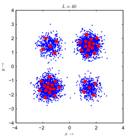
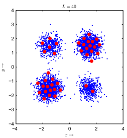
In the next step, we approximate samples from a Gaussian mixture density. For that purpose, we generated samples from a Gaussian mixture density with four components, see Fig. 2. It is important to note that we have a total of $M=4000$ samples, but the number of samples differs for each component: We have $500$ samples for components $(1,1)$ and $(2,2)$ and $1500$ samples for components $(1,2)$ and $(2,1)$. After the reduction from $M=4000$ samples down to $L=40$ samples, we would expect that the probability masses for each component of the Gaussian mixture density are maintained. This is exactly the case for the proposed LCD reduction as can be seen in Fig. 2 on the left side, where we end up with $5$ samples for components $(1,1)$ and $(2,2)$ and $15$ samples for components $(1,2)$ and $(2,1)$. For k-means clustering, shown on the right side in Fig. 2, this is not the case, so the original distribution is not maintained. In addition, the results of k-means clustering are not reproducible and change with every run.

Figure 2: Reduction of a Gaussian mixture density with four components and a varying number of samples per component from $4000$ points to $40$ points. Blue: Random samples representing the Gaussian mixture density. Red: Reduced point set. (left) LCD reduction. (right) Result of k-means clustering.

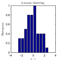
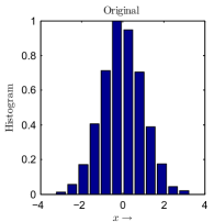
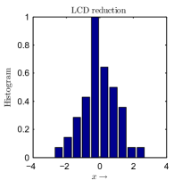
Another way to demonstrate that the proposed reduction method maintains the probability mass distribution is to compare histograms of the samples before and after reduction. To simplify visualization, histograms are calculated for the marginals in $x$-direction. Fig. 3 shows the histogram of the originals samples on the left side. The histogram after reduction with the proposed LCD reduction method is shown in the middle, while the histogram of the results obtained with k-means are shown on the right side. It is obvious that the histogram of the LCD reduction is much closer to the original histogram than the histogram of k-means.

Figure 3: Normalized histograms of projections onto $x$-axis for reducing $M=5000$ samples of a two-dimensional standard normal distribution to $L=50$ samples. (left) Marginal of original samples. (middle) Marginal of LCD reduction result. (right) Marginal of result of k-means clustering.

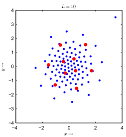
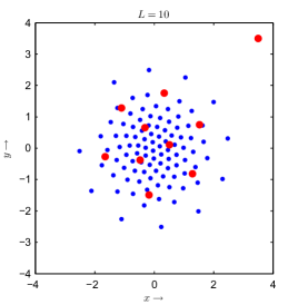
We now consider $M=100$ deterministic samples of a standard Normal distribution shown in Fig. 4. The samples are calculated with the method from CDC09_HanebeckHuber . One sample is replaced with an outlier located at $[3.5,3.5]^{T}$. The point set is reduced to $L=10$ samples. The left side shows the result of the LCD reduction. The samples are well placed and only slightly shifted due to the outlier. On the right side, k-means clustering produces a result heavily disturbed by the outlier. In fact, one sample of the reduced point set is placed directly on the outlier, which significantly changes the mass distribution. Instead of representing $1$ % of the distribution as before the reduction, the outlier now allocates $10$ %.

Figure 4: Blue: Deterministic samples representing a standard Normal distribution. One sample is replaced by an outlier at $[3.5,3.5]^{T}$. Red: Reduced point set. (left) LCD reduction. (right) k-means clustering.

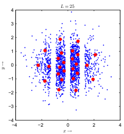
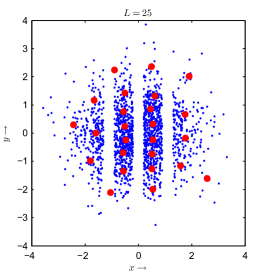
Finally, we investigate the robustness of the reduction methods with respect to missing data. For that purpose, we generate $2500$ samples and remove samples located within three vertical strips, see Fig. 5. The remaining samples are reduced down to $L=25$ samples. Fig. 5 left shows the result of the LCD reduction, which almost gives the same results as before. The right side shows the result of k-means clustering, where it is obvious that samples are more or less placed along lines and the original mass distribution is not well maintained.

Figure 5: Blue: Random samples representing a standard Normal distribution with some samples removed along three vertical lines. Red: Reduced point set. (left) LCD reduction. (right) k-means clustering.

8 Discussion

A systematic approach for approximating a given Dirac mixture density by another one with less components has been introduced that is radically different from current clustering or vector quantization approaches. The (weights and) locations of the approximating density are calculated by minimizing a global distance measure, a generalization of the well-known Cramér-von Mises Distance to the multivariate case. This generalization is obtained by defining an alternative to the classical cumulative distribution, the Localized Cumulative Distribution (LCD), as a characterization of discrete random quantities, which is unique and symmetric also in the multivariate case.

Although kernels are used to define the LCD, this is not a kernel method. The distance measure is obtained by integrating over all possible kernels with all locations and widths, so that the final expression does not contain any kernel.

The given Dirac mixture might be the result from random sampling or from certain processing steps involving analytic Dirac mixtures. In any case, the resulting approximating Dirac mixture is fully deterministic and the optimization process gives reproducible results.

Compared to clustering methods that find cluster heads minimizing the distance to their nearest neighbors, which is a local method, the LCD reduction globally matches the mass distributions of the given point set and its approximation. This leads to a smooth distance measure with almost no local minima that can be efficiently minimized with standard optimization procedures. However, it is important to note that due to its operating principle the proposed reduction method does not provide a mapping from old components to new components.

Constraints on the state variables can easily be considered when performing the approximation of the given density. An obvious application is the explicit avoidance of certain regions in the state space in order to obey certain physical constraints. However, an even more interesting application is the interpretation of the measurement equation in the Bayesian filtering step as an equality constraint for the state variables once an actual observation is available. This opens the way for more advanced filtering techniques in the case of Dirac mixture densities other than reweighing the individual component by the likelihood function.

Large data sets occur when performing Dirac mixture based state estimation in high–dimensional spaces or when considering product spaces of Dirac mixture densities. For a very large number of components, the computational effort for performing a direct reduction might be too large. For coping with this complexity issue, the proposed approach offers the unique feature of hierarchical approximation. For that purpose, the data set is decomposed into several smaller sets that are individually approximated. The resulting Dirac components of the individual approximations are then collected into a single approximating Dirac mixture, which subsequently is further approximated to yield the desired number of components. Of course, this approximation hierarchy may consist of more intermediate approximation steps.

Appendix A Gradient of Distance Measure

Taking the derivative of the distance measure in (2) with respect to a location $x_{\xi}^{(\eta)}$ gives

$$G_{\xi}^{(\eta)}=\frac{\partial D}{\partial x_{\xi}^{(\eta)}}=-2\int_{0}^{b_{\text{max}}}\frac{1}{b^{N-1}}\int_{\mathbb{R}^{N}}\left(\tilde{F}(\underline{m},b)-F(\underline{m},b)\right)\frac{\partial F(\underline{m},b)}{\partial x_{\xi}^{(\eta)}}\,d\underline{m}\,db\enspace,$$

with

$$\frac{\partial F(\underline{m},b)}{\partial x_{\xi}^{(\eta)}}=-w_{\xi}^{x}\,\frac{x_{\xi}^{(\eta)}-m^{(\eta)}}{b^{2}}\prod_{k=1}^{N}\exp\left(-\frac{1}{2}\frac{\left(x_{\xi}^{(k)}-m^{(k)}\right)^{2}}{b^{2}}\right)\enspace.$$

In the following, the two parts of $G_{\xi}^{(\eta)}$ will be treated seperatly according to

$$G_{\xi}^{(\eta)}=G_{\xi}^{(\eta,1)}-G_{\xi}^{(\eta,2)}\enspace{.}$$ (6)

The first part is given by

$$G_{\xi}^{(\eta,1)}=-2\int_{0}^{b_{\text{max}}}\frac{1}{b^{N-1}}\int_{\mathbb{R}^{N}}\tilde{F}(\underline{m},b)\frac{\partial F(\underline{m},b)}{\partial x_{\xi}^{(\eta)}}\,d\underline{m}\,db\enspace.$$

By using the expressions for $\tilde{F}(\underline{m},b)$ and $\frac{\partial F(\underline{m},b)}{\partial x_{\xi}^{(\eta)}}$, we obtain

$$\begin{split}G_{\xi}^{(\eta,1)}=2w_{\xi}^{x}\,\int_{0}^{b_{\text{max}}}\frac{1}{b^{N-1}}\int_{\mathbb{R}^{N}}\frac{x_{\xi}^{(\eta)}-m^{(\eta)}}{b^{2}}&\prod_{k=1}^{N}\exp\left(-\frac{1}{2}\frac{\left(x_{\xi}^{(k)}-m^{(k)}\right)^{2}}{b^{2}}\right)\\ \sum_{i=1}^{M}w_{i}^{y}&\prod_{k=1}^{N}\exp\left(-\frac{1}{2}\frac{(y_{i}^{(k)}-m^{(k)})^{2}}{b^{2}}\right)d\underline{m}\,db\end{split}\enspace.$$

Combining the product terms gives

$$\begin{split}G_{\xi}^{(\eta,1)}=2\,w_{\xi}^{x}\sum_{i=1}^{M}w_{i}^{y}\int_{0}^{b_{\text{max}}}\frac{1}{b^{N-1}}\int_{\mathbb{R}}\frac{x_{\xi}^{(\eta)}-m^{(\eta)}}{b^{2}}&\exp\left(-\frac{1}{2}\frac{\left(x_{\xi}^{(\eta)}-m^{(\eta)}\right)^{2}}{b^{2}}\right)\\ &\exp\left(-\frac{1}{2}\frac{(y_{i}^{(\eta)}-m^{(\eta)})^{2}}{b^{2}}\right)dm^{(\eta)}\\ \prod_{\stackrel{{\scriptstyle k=1}}{{k\neq\eta}}}^{N}\int_{\mathbb{R}}&\exp\left(-\frac{1}{2}\frac{\left(x_{\xi}^{(k)}-m^{(k)}\right)^{2}}{b^{2}}\right)\\ &\exp\left(-\frac{1}{2}\frac{(y_{i}^{(k)}-m^{(k)})^{2}}{b^{2}}\right)dm^{(k)}db\end{split}\enspace.$$

For further simplification, the equality

$$\begin{gathered}\int_{\mathbb{R}}\frac{z_{i}-m}{b^{2}}\exp\left(-\frac{1}{2}\frac{(z_{i}-m)^{2}}{b^{2}}\right)\exp\left(-\frac{1}{2}\frac{(z_{j}-m)^{2}}{b^{2}}\right)dm\\ =\sqrt{\pi}\,\frac{z_{i}-z_{j}}{2\,b}\exp\left(-\frac{1}{2}\frac{(z_{i}-z_{j})^{2}}{2\,b^{2}}\right)\end{gathered}$$

is used together with the equality (3), which leads to

$$\begin{split}G_{\xi}^{(\eta,1)}=&\pi^{\frac{N}{2}}\,w_{\xi}^{x}\sum_{i=1}^{M}w_{i}^{y}\left(x_{\xi}^{(\eta)}-y_{i}^{(\eta)}\right)\\ &\int_{0}^{b_{\text{max}}}\frac{1}{b}\prod_{k=1}^{N}\exp\left(-\frac{1}{2}\frac{\left(x_{\xi}^{(k)}-y_{i}^{(k)}\right)^{2}}{2\,b^{2}}\right)db\end{split}$$

or equivalently to

$$\begin{split}G_{\xi}^{(\eta,1)}=&\pi^{\frac{N}{2}}\,w_{\xi}^{x}\sum_{i=1}^{M}w_{i}^{y}\left(x_{\xi}^{(\eta)}-y_{i}^{(\eta)}\right)\\ &\int_{0}^{b_{\text{max}}}\frac{1}{b}\exp\left(-\frac{1}{2}\frac{\displaystyle\sum_{k=1}^{N}\left(x_{\xi}^{(k)}-y_{i}^{(k)}\right)^{2}}{2\,b^{2}}\right)db\end{split}\enspace.$$

With

$$\int_{0}^{b_{\text{max}}}\frac{1}{b}\,\exp\left(-\frac{1}{2}\frac{z}{2\,b^{2}}\right)\,db=-\frac{1}{2}\,\operatorname{Ei}\left(-\frac{1}{2}\frac{z}{2\,b_{\text{max}}^{2}}\right)$$

for $z>0$, the expression

$$\frac{\partial D}{\partial x_{\xi}^{(\eta)}}=\frac{\pi^{\frac{N}{2}}}{2}w_{\xi}^{x}\sum_{i=1}^{L}w_{i}^{x}\left(x_{\xi}^{(\eta)}-x_{i}^{(\eta)}\right)\operatorname{Ei}\left(-\frac{1}{2}\frac{\displaystyle\sum_{k=1}^{N}\left(x_{\xi}^{(k)}-y_{i}^{(k)}\right)^{2}}{2b_{\text{max}}^{2}}\right)$$

is obtained for component index $\xi=1,\ldots,L$ and dimension index $k=1,\ldots,N$.

The second part is given by

$$G_{\xi}^{(\eta,2)}=-2\int_{0}^{b_{\text{max}}}\frac{1}{b^{N-1}}\int_{\mathbb{R}^{N}}F(\underline{m},b)\frac{\partial F(\underline{m},b)}{\partial x_{\xi}^{(\eta)}}\,d\underline{m}\,db\enspace.$$

By using the expressions for $F(\underline{m},b)$ and $\frac{\partial F(\underline{m},b)}{\partial x_{\xi}^{(\eta)}}$, we obtain

$$\begin{split}G_{\xi}^{(\eta,2)}=2w_{\xi}^{x}\,\int_{0}^{b_{\text{max}}}&\frac{1}{b^{N-1}}\int_{\mathbb{R}^{N}}\\ \frac{x_{\xi}^{(\eta)}-m^{(\eta)}}{b^{2}}&\prod_{k=1}^{N}\exp\left(-\frac{1}{2}\frac{\left(x_{\xi}^{(k)}-m^{(k)}\right)^{2}}{b^{2}}\right)\\ \sum_{i=1}^{L}w_{i}^{x}&\prod_{k=1}^{N}\exp\left(-\frac{1}{2}\frac{(x_{i}^{(k)}-m^{(k)})^{2}}{b^{2}}\right)d\underline{m}\,db\end{split}\enspace.$$

Combining the product terms gives

$$\begin{split}G_{\xi}^{(\eta,2)}=2\,w_{\xi}^{x}\sum_{i=1}^{L}w_{i}^{x}\int_{0}^{b_{\text{max}}}\frac{1}{b^{N-1}}\int_{\mathbb{R}}\frac{x_{\xi}^{(\eta)}-m^{(\eta)}}{b^{2}}&\exp\left(-\frac{1}{2}\frac{\left(x_{\xi}^{(\eta)}-m^{(\eta)}\right)^{2}}{b^{2}}\right)\\ &\exp\left(-\frac{1}{2}\frac{(x_{i}^{(\eta)}-m^{(\eta)})^{2}}{b^{2}}\right)dm^{(\eta)}\\ \prod_{\stackrel{{\scriptstyle k=1}}{{k\neq\eta}}}^{N}\int_{\mathbb{R}}&\exp\left(-\frac{1}{2}\frac{\left(x_{\xi}^{(k)}-m^{(k)}\right)^{2}}{b^{2}}\right)\\ &\exp\left(-\frac{1}{2}\frac{(x_{i}^{(k)}-m^{(k)})^{2}}{b^{2}}\right)dm^{(k)}db\end{split}\enspace.$$

For further simplification, we use

$$\int_{\mathbb{R}}\frac{z_{i}-m}{b^{2}}\exp\left(-\frac{1}{2}\frac{(z_{i}-m)^{2}}{b^{2}}\right)\exp\left(-\frac{1}{2}\frac{(z_{j}-m)^{2}}{b^{2}}\right)dm=\sqrt{\pi}\,\frac{z_{i}-z_{j}}{2\,b}\exp\left(-\frac{1}{2}\frac{(z_{i}-z_{j})^{2}}{2\,b^{2}}\right)$$

and (3), which leads to

$$G_{\xi}^{(\eta,2)}=\pi^{\frac{N}{2}}\,w_{\xi}^{x}\sum_{i=1}^{L}w_{i}^{x}\left(x_{\xi}^{(\eta)}-x_{i}^{(\eta)}\right)\int_{0}^{b_{\text{max}}}\frac{1}{b}\prod_{k=1}^{N}\exp\left(-\frac{1}{2}\frac{\left(x_{\xi}^{(k)}-x_{i}^{(k)}\right)^{2}}{2\,b^{2}}\right)db\enspace.$$

or equivalently

$$G_{\xi}^{(\eta,2)}=\pi^{\frac{N}{2}}\,w_{\xi}^{x}\sum_{i=1}^{L}w_{i}^{x}\left(x_{\xi}^{(\eta)}-x_{i}^{(\eta)}\right)\int_{0}^{b_{\text{max}}}\frac{1}{b}\exp\left(-\frac{1}{2}\frac{\displaystyle\sum_{k=1}^{N}\left(x_{\xi}^{(k)}-x_{i}^{(k)}\right)^{2}}{2\,b^{2}}\right)db\enspace.$$

With

$$\int_{0}^{b_{\text{max}}}\frac{1}{b}\,\exp\left(-\frac{1}{2}\frac{z}{2\,b^{2}}\right)\,db=-\frac{1}{2}\,\operatorname{Ei}\left(-\frac{1}{2}\frac{z}{2\,b_{\text{max}}^{2}}\right)$$

for $z>0$, we obtain

$$G_{\xi}^{(\eta,2)}=\frac{\pi^{\frac{N}{2}}}{2}w_{\xi}^{x}-\sum_{i=1}^{M}w_{i}^{y}\left(x_{\xi}^{(\eta)}-y_{i}^{(\eta)}\right)\operatorname{Ei}\left(-\frac{1}{2}\frac{\displaystyle\sum_{k=1}^{N}\left(x_{\xi}^{(k)}-x_{i}^{(k)}\right)^{2}}{2b_{\text{max}}^{2}}\right)$$

for component index $\xi=1,\ldots,L$ and dimension index $k=1,\ldots,N$.

By combining the two results for $G_{\xi}^{(\eta,1)}$ and $G_{\xi}^{(\eta,2)}$ according to (6), we obtain the following Theorem.

Theorem A.1.

The gradient of the general distance measure in Theorem 4.1 with respect to the locations of the Dirac components is given by

$$\begin{split}\frac{\partial D}{\partial x_{\xi}^{(\eta)}}=\frac{\pi^{\frac{N}{2}}}{2}w_{\xi}^{x}\Bigg{\{}\sum_{i=1}^{L}&w_{i}^{x}\left(x_{\xi}^{(\eta)}-y_{i}^{(\eta)}\right)\operatorname{Ei}\left(-\frac{1}{2}\frac{\displaystyle\sum_{k=1}^{N}\left(x_{\xi}^{(k)}-y_{i}^{(k)}\right)^{2}}{2b_{\text{max}}^{2}}\right)\\ -\sum_{i=1}^{M}&w_{i}^{y}\left(x_{\xi}^{(\eta)}-x_{i}^{(\eta)}\right)\operatorname{Ei}\left(-\frac{1}{2}\frac{\displaystyle\sum_{k=1}^{N}\left(x_{\xi}^{(k)}-x_{i}^{(k)}\right)^{2}}{2b_{\text{max}}^{2}}\right)\Bigg{\}}\end{split}$$

for component index $j=1,\ldots,L$ and dimension index $k=1,\ldots,N$.

For large $b_{\text{max}}$, the $\operatorname{Ei}$–function in Theorem A.1 can be approximated according to (5). Hence, we have

$$\begin{split}\operatorname{Ei}\left(-\frac{z}{4\,b_{\text{max}}^{2}}\right)&\approx\Gamma-\frac{z}{4\,b_{\text{max}}^{2}}+\log\left(\frac{z}{4\,b_{\text{max}}^{2}}\right)\\ &\approx\Gamma-\log\left(4\,b_{\text{max}}^{2}\right)+\log(z)\\ &=-C_{b}+\log(z)\end{split}$$

for $z>0$. With

$$\begin{gathered}-C_{b}\left\{\sum_{i=1}^{L}w_{i}^{x}\left(x_{\xi}^{(\eta)}-x_{i}^{(\eta)}\right)-\sum_{i=1}^{M}w_{i}^{y}\left(x_{\xi}^{(\eta)}-y_{i}^{(\eta)}\right)\right\}\\ =C_{b}\left(\sum_{i=1}^{L}w_{i}^{x}x_{i}^{(\eta)}-\sum_{i=1}^{M}w_{i}^{y}y_{i}^{(\eta)}\right)\enspace,\end{gathered}$$

we obtain the next Theorem.

Theorem A.2.

For large $b_{\text{max}}$, the gradient of the distance measure with respect to the locations of the Dirac components is given by

$$\begin{split}\frac{\partial D}{\partial x_{\xi}^{(\eta)}}=\frac{\pi^{\frac{N}{2}}}{2}w_{\xi}^{x}&\left\{\sum_{i=1}^{L}w_{i}^{x}\left(x_{\xi}^{(\eta)}-x_{i}^{(\eta)}\right)\log\left(\sum_{k=1}^{N}\left(x_{\xi}^{(k)}-x_{i}^{(k)}\right)^{2}\right)\right.\\ -&\sum_{i=1}^{M}w_{i}^{y}\left(x_{\xi}^{(\eta)}-y_{i}^{(\eta)}\right)\log\left(\sum_{k=1}^{N}\left(x_{\xi}^{(k)}-y_{i}^{(k)}\right)^{2}\right)\\ +&C_{b}\cdot\left.\left(\sum_{i=1}^{L}w_{i}^{x}x_{i}^{(\eta)}-\sum_{i=1}^{M}w_{i}^{y}y_{i}^{(\eta)}\right)\right\}\enspace,\end{split}$$ (7)

for component index $\xi=1,\ldots,L$ and dimension index $\eta=1,\ldots,N$.

Corollary A.3.

For equal expected values, the optimal locations $\underline{x}_{i}=\begin{bmatrix}x_{i},y_{i}\end{bmatrix}^{T}$ of the components $i=1,\ldots,L$ of the approximating Dirac mixture density are obtained by solving the following $N\cdot L$ equations (necessary conditions)

$$\begin{split}&\sum_{i=1}^{M}w_{i}^{y}\left(x_{\xi}^{(\eta)}-y_{i}^{(\eta)}\right)\log\left(\sum_{k=1}^{N}\left(x_{\xi}^{(k)}-y_{i}^{(k)}\right)^{2}\right)\\ =&\sum_{i=1}^{L}w_{i}^{x}\left(x_{\xi}^{(\eta)}-x_{i}^{(\eta)}\right)\log\left(\sum_{k=1}^{N}\left(x_{\xi}^{(k)}-x_{i}^{(k)}\right)^{2}\right)\enspace,\end{split}$$ (8)

for component index $\xi=1,\ldots,L$ and dimension index $\eta=1,\ldots,N$.

References

• (1) S.Β Lloyd, β€œLeast squares quantization in PCM,” IEEE Transactions on Information Theory, vol.Β 28, no.Β 2, pp. 129–137, Mar. 1982.
• (2) J.Β MacQueen, β€œSome methods for classification and analysis of multivariate observations.”   The Regents of the University of California, 1967. [Online]. Available: http://projecteuclid.org/euclid.bsmsp/1200512992
• (3) Y.Β Linde, A.Β Buzo, and R.Β Gray, β€œAn Algorithm for Vector Quantizer Design,” IEEE Transactions on Communications, vol.Β 28, no.Β 1, pp. 84–95, Jan. 1980.
• (4) D.Β Crouse, P.Β Willett, K.Β Pattipati, and L.Β Svensson, β€œA look at Gaussian mixture reduction algorithms,” in 2011 Proceedings of the 14th International Conference on Information Fusion (FUSION), Jul. 2011, pp. 1–8.
• (5) J.Β Williams and P.Β Maybeck, β€œCost-Function-Based Gaussian Mixture Reduction for Target Tracking,” in Proceedings of the Sixth International Conference of Information Fusion, 2003, vol.Β 2, Jul. 2003, pp. 1047–1054.
• (6) A.Β Runnalls, β€œKullback-Leibler Approach to Gaussian Mixture Reduction,” IEEE Transactions on Aerospace and Electronic Systems, vol.Β 43, no.Β 3, pp. 989–999, Jul. 2007.
• (7) U.Β D. Hanebeck and V.Β Klumpp, β€œLocalized Cumulative Distributions and a Multivariate Generalization of the CramΓ©r-von Mises Distance,” in Proceedings of the 2008 IEEE International Conference on Multisensor Fusion and Integration for Intelligent Systems (MFI 2008), Seoul, Republic of Korea, Aug. 2008, pp. 33–39.
• (8) M.Β West, β€œApproximating Posterior Distributions by Mixture,” Journal of the Royal Statistical Society. Series B (Methodological), vol.Β 55, no.Β 2, pp. 409–422, Jan. 1993. [Online]. Available: http://www.jstor.org/stable/2346202
• (9) T.Β Lefebvre, H.Β Bruyninckx, and J.Β DeΒ Schutter, β€œThe Linear Regression Kalman Filter,” in Nonlinear Kalman Filtering for Force-Controlled Robot Tasks, ser. Springer Tracts in Advanced Robotics, 2005, vol.Β 19.
• (10) S.Β Julier, J.Β Uhlmann, and H.Β F. Durrant-Whyte, β€œA New Method for the Nonlinear Transformation of Means and Covariances in Filters and Estimators,” IEEE Transactions on Automatic Control, vol.Β 45, no.Β 3, pp. 477–482, Mar. 2000.
• (11) S.Β J. Julier, β€œThe Scaled Unscented Transformation,” in Proceedings of the 2002 IEEE American Control Conference (ACC 2002), vol.Β 6, Anchorage, Alaska, USA, May 2002, pp. 4555– 4559.
• (12) D.Β Tenne and T.Β Singh, β€œThe Higher Order Unscented Filter,” in Proceedings of the 2003 IEEE American Control Conference (ACC 2003), vol.Β 3, Denver, Colorado, USA, Jun. 2003, pp. 2441–2446.
• (13) M.Β F. Huber and U.Β D. Hanebeck, β€œGaussian Filter based on Deterministic Sampling for High Quality Nonlinear Estimation,” in Proceedings of the 17th IFAC World Congress (IFAC 2008), vol.Β 17, no.Β 2, Seoul, Republic of Korea, Jul. 2008.
• (14) G.Β Kurz, I.Β Gilitschenski, and U.Β D. Hanebeck, β€œRecursive Nonlinear Filtering for Angular Data Based on Circular Distributions,” in Proceedings of the 2013 American Control Conference (ACC 2013), Washington D. C., USA, Jun. 2013.
• (15) I.Β Gilitschenski, G.Β Kurz, and U.Β D. Hanebeck, β€œBearings-Only Sensor Scheduling Using Circular Statistics,” in Proceedings of the 16th International Conference on Information Fusion (Fusion 2013), Istanbul, Turkey, Jul. 2013.
• (16) G.Β Kurz, F.Β Faion, and U.Β D. Hanebeck, β€œConstrained Object Tracking on Compact One-dimensional Manifolds Based on Directional Statistics,” in Proceedings of the Fourth IEEE GRSS International Conference on Indoor Positioning and Indoor Navigation (IPIN 2013), Montbeliard, France, Oct. 2013.
• (17) U.Β D. Hanebeck, β€œTruncated Moment Problem for Dirac Mixture Densities with Entropy Regularization,” arXiv preprint: Systems and Control (cs.SY), Aug. 2014. [Online]. Available: http://arxiv.org/abs/1408.7083
• (18) O.Β C. Schrempf, D.Β Brunn, and U.Β D. Hanebeck, β€œDensity Approximation Based on Dirac Mixtures with Regard to Nonlinear Estimation and Filtering,” in Proceedings of the 2006 IEEE Conference on Decision and Control (CDC 2006), San Diego, California, USA, Dec. 2006.
• (19) β€”β€”, β€œDirac Mixture Density Approximation Based on Minimization of the Weighted CramΓ©r-von Mises Distance,” in Proceedings of the 2006 IEEE International Conference on Multisensor Fusion and Integration for Intelligent Systems (MFI 2006), Heidelberg, Germany, Sep. 2006, pp. 512–517.
• (20) U.Β D. Hanebeck, M.Β F. Huber, and V.Β Klumpp, β€œDirac Mixture Approximation of Multivariate Gaussian Densities,” in Proceedings of the 2009 IEEE Conference on Decision and Control (CDC 2009), Shanghai, China, Dec. 2009.
• (21) I.Β Gilitschenski and U.Β D. Hanebeck, β€œEfficient Deterministic Dirac Mixture Approximation,” in Proceedings of the 2013 American Control Conference (ACC 2013), Washington D. C., USA, Jun. 2013.
• (22) H.Β Eberhardt, V.Β Klumpp, and U.Β D. Hanebeck, β€œOptimal Dirac Approximation by Exploiting Independencies,” in Proceedings of the 2010 American Control Conference (ACC 2010), Baltimore, Maryland, USA, Jun. 2010.
• (23) W.Β H. Press, S.Β A. Teukolsky, W.Β T. Vetterling, and B.Β P. Flannery, Numerical Recipes in C (2Nd Ed.): The Art of Scientific Computing.Β Β Β New York, NY, USA: Cambridge University Press, 1992.