TaxMan: an online facility for the coding of continuous characters for cladistic analysis

¹ Centre for Research in Evolutionary Anthropology,
School of Human and Life Sciences, Roehampton University,
Holybourne Avenue, London SW15 4JD,
UNITED KINGDOM;
t.rae@roehampton.ac.uk
² School of Physics & Astronomy,
University of Glasgow, Glasgow G12 7QQ,
UNITED KINGDOM;
formerly at
Centre for Particle Theory, Department of Physics,
Durham University, South Road, Durham DH1 3LE,
UNITED KINGDOM;

1 Introduction

Human nature is, above all things, lazy.

— Harriet Beecher Stowe,
         — Household Papers and Stories, 1864, ch. 6

It is generally agreed that the bulk of morphological variation in organisms is quantitative, even if it is described at times as if it were meristic or qualitative (Pogue and Mickevich, 1990; Stevens, 1991). Although objections to the use of quantitative traits in phylogenetic systematics have been raised in the past (Crisp and Weston, 1987; Pimentel and Riggins, 1987), these have been shown to be spurious (Rae, 1998). There is an emerging consensus that quantitative variation can (and should) be used in cladistics (Garcia-Cruz and Sosa, 2006), but there is no agreement on the method(s) that should be used to translate numerical data into data matrices amenable to computer-based analysis, and several different methods have been suggested (Simon, 1983; Thiele, 1993; Strait et al., 1996; Goloboff et al., 2004).

To a greater or lesser extent, however, the bulk of the methods proposed to date for coding quantitative data for cladistic analysis include arbitrary aspects (Rae, 1998), which limits their applicability to scientific enquiry. This objection applies to all forms of segment- or gap-coding, where there is no objective a priori criterion for deciding segment size or gap size threshold. All previously published “tests” of the efficacy of different methods of coding rely on comparisons between topologies produced by various coding methods (or continuous vs. “non-continuous” data); that the choice of coding method can affect the resulting cladograms is a given, but comparing trees does not reveal whether any particular coding method accurately reflects variation. For example, while results of comparisons between identical data coded using different systems may reveal that one method produces a “small number of well-resolved trees with strong bootstrap support” (Garcia-Cruz and Sosa, 2006: 302), this does necessarily mean that the results reflect the evolution of the organisms accurately; the resultant “good” behaviour may be simply an incidental by-product of the method. For example, it may be that a particular method simply creates more character states (and hence more apparent resolution) because the number of states created is arbitrarily equal to the maximum number of states allowed by the tree-searching software used (Thiele, 1993); thus, there could be more distinctions between taxa, and perhaps even fewer equally parsimonious minimum-length trees, but the distinctions would be illusory. In addition, it has been shown (Mickevich and Farris, 1981) that methods which add an element of scaling to the coding procedure treat every character as if it has changed by the same (arbitrary) degree as every other trait, a situation not likely to have occurred many times in the course of the evolution of life.

Coding methods based on statistical tests between taxa suffer from no such drawbacks. There is no arbitrary (and thus infinitely variable) gap size threshold and the number of character states is determined by the statistical differences between taxa, not by the limitations of phylogenetic software (Rae, 1998). Surprisingly, however, these techniques are rarely used, probably because they are difficult to implement using existing computer programs.

On the other hand, gap-weighting (Thiele and Ladiges, 1988) is a popular method for coding quantitative characters (e.g., Torres-Carvajal, 2007), despite the objections against it (see above). This may be due to the fact that there is software (Morphocode) that is specifically designed to translate metric data into Nexus-format files (Schols et al., 2004). A recent implementation of a modified version of gap-coding method is now available in TNT, as well (Goloboff et al., 2004); this method, although touted as treating “continuous characters as such” (Goloboff et al., 2004: 589), simply assigns a step (or part thereof) corresponding to the distance between means or where the “ranges” of taxa do not overlap. In this case, the arbitrary element is not introduced by gap size, but by the characterisation of the range, which is “up to the user” (Goloboff et al., 2004: 591). If the advent of computer algorithms has taught us nothing else, it is that the available software will be applied to a problem regardless of whether it is appropriate; hence the continued reporting of majority-rule consensus trees (e.g., Belfiore et al., 2008) long after they have been shown to be suspect from first principles (Sharkey and Leathers, 2001).

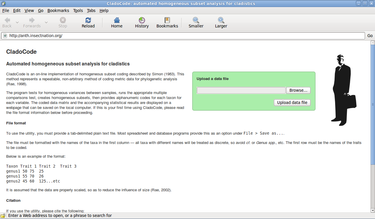
To address this shortcoming, the present contribution outlines a new Web-based package that can be used to code numerical data for phylogenetic analysis. TaxMan (http://anth.insectnation.org) is an implementation of the Homogeneous Subset Coding (HSC) method (Simon, 1983) that can be run via any Web browser (Figure 1). Analogous to ClustalW (Higgins et al., 1994), the Web-based sequence alignment site (http://www.ebi.ac.uk/Tools/clustalw2/), TaxMan allows the entry of data from which the algorithm will produce a data matrix amenable to tree-searching computer software such as PAUP* (Swofford, 2003) or TNT (Goloboff et al., 2003; Goloboff et al., 2008).

2 Methods

TaxMan proceeds by evaluating the data using standard statistical methods (Sokal and Rohlf, 1981). For each trait, homogeneity of variances is determined with Bartlett’s test. Traits with homogeneous variances are then subjected to the parametric GT2 multiple comparisons test. Characters demonstrating non-homogeneous variances are evaluated using the non-parametric Games and Howell procedure. As the multiple comparisons procedures are post-hoc, two-tailed tests are used throughout. The standard critical value of $p<0.05$ is utilised for all of the calculations. Taxa are sorted into homogeneous subsets (i.e., those taxa that do not differ significantly from each other), and all taxa belonging to exactly the same subsets are assigned the same code. The procedure is identical to that of Simon (1983), with the exception that codes are represented by single alphanumeric characters only (0-9, a-z, and A-Z). The resulting data matrix is sorted with taxa arranged vertically and characters positioned along the horizontal axis. Details of the statistical algorithms and their implementation are given in the Appendix.

3 Worked example

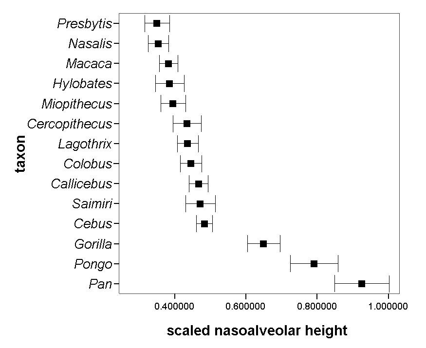
To illustrate the applicability of TaxMan, a linear measurement of the facial skeleton of anthropoids (Mammalia: Primates), previously utilised in phylogenetic analysis of the group (Rae, 1993), is analysed below. The length of the nasoalveolar clivus (measured from prosthion to the anterior nasal spine) has been hypothesised to distinguish great apes (Hominidae, including the extant genera Pongo, Pan, Gorilla, and Homo) from other anthropoid primates (Harrison, 1982; Rae, 1997; Rae, 1999). Data from 19–20 individuals each from 15 extant genera were taken with digital sliding callipers accurate to $0.01\text{\,}\mathrm{mm}$. The individual variates were scaled by dividing each value by a grand mean of 12 measurements taken from the same individual (Jungers et al., 1995). The scaled variates (Figure 2) were coded via TaxMan, and compared with codings and treatments from both Morphocode, which implements a gap-weighting coding algorithm (Thiele, 1993), and the continuous data option (Goloboff et al., 2004) of TNT. Morphocode allows the number of character states in the coding to vary between the two default settings (10, 26); only these two settings were used. The “cont” algorithm of TNT (Goloboff et al., 2003) does not code data as such, so two alternative ways of entering continuous data allowed by the program (means, ranges) were implemented. These were added to an identical string of identical dummy variables, so that the resulting cladograms (and character weightings) differ only due to the influence of the single continuous character. Descriptive statistics were derived using SPSS for Windows, version 15.0 (SPSS Inc., Chicago).

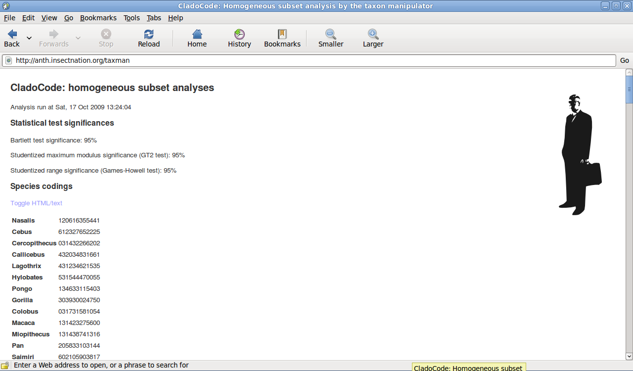
The coding of the scaled data by the various methods is given in Table 1. The results from TaxMan consist of a single set of codes for the taxa analysed. There are six states (0–5) and the hominids are characterised by an elevated value. The mean values were analysed with Morphocode, using the $n=10$ states and $n=26$ states settings. As Morphocode uses non-alphanumeric characters as codes between the integers and letters, to facilitate the comparison with TaxMan all states greater than 9 were translated into their alphanumeric equivalents. It is obvious that the number of states chosen affects the resulting states directly; whereas Callicebus and Cebus were deemed to be the “same” in the $n=10$ states coding (both state 2), they are “different” in $n=26$ states analysis (states 5 and 6, respectively). Similarly, Cercopithecus, Colobus, Hylobates, Lagothrix, Macaca, and Miopithecus are indistinguishable in the first run and spread across three states in the second. Other alternative codings can be obtained by choosing intermediate values for the number of states. All of these distinctions are arbitrary and have nothing to do with the morphometric qualities of the organisms.

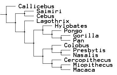
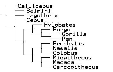
Two additional tests were conducted by adding alternatively a) taxon means and b) 68% confidence intervals (mean $\pm$ one standard deviation) to an artificial matrix (Table 2) for analysis in TNT using the “nstates cont” option (Figure 3). This method does not allow a direct comparison to TaxMan, as there are no codings per se to contrast, but the two options used produce different topologies and numbers of steps produced for the one continuous character. The “means” run showed more resolution, splitting several polytomies seen in the “ranges” run, implying that the former strategy produces synapomorphies not discovered in the latter. Also, the continuous character introduced more steps (or fractions thereof) in the “means” run (0.877 steps) than the “range” run (0.358 steps). Thus, although the data had not changed, both the Morphocode and the “analyzing continuous characters as such” methods produce results that differ, depending on the arbitrary choice of number of states or method of entry.

4 Discussion

Much has been made, by workers advocating coding methods for phylogenetics, of the observation that including measurement data in phylogenetic analyses increases information content (Chappill, 1989). While this is undoubtedly true, it is probably trivial; the inclusion of any additional data could also increase the resolution/support for various clades. As was found with PTP tests (Slowinski and Corhter, 1998) and other measures of “phylogenetic content”, there are likely to be very few observations of organisms that cannot provide phylogenetic information of some sort. The central issue of coding should be that it provides a way of including metric data without resorting to arbitrary thresholds or ranges.

One objection that has been raised with respect to coding methods is that they may allow the separation of taxa with mean values for a particular character that are not significantly different from one another (Farris, 1990). In HSC, this is implemented via the coding of intermediates: if the means of taxa A and C are significantly different for a trait, but taxon B has a mean that lies between those of A and C, but is not significantly different from either, taxon B is coded as intermediate. As pointed out previously (Swiderski et al., 1998), this is exactly the distribution that would be expected in a trait changing via gradualism; to argue that this “creates non-existent differences” is to ignore the obvious power of selection on populations. The alternative in multiple comparisons is to place all three in the same category, even though demonstrable differences occur within. The default assumption should be that any information on distinctions between taxa is relevant for phylogeny and should be included, rather than ignored.

A second but related issue in cladistic coding for involves the scaling of metric traits. An organism’s size is one of its most fundamental adaptations (Jungers, 1985). A good deal of variance in any metric assessment of a group of organisms will be directly attributable to size alone. Raw (or even incorrectly scaled) measurements will introduce an element of non-independence in cladistic analysis (Rae, 2002), violating one of the fundamental assumptions of the methods of phylogenetic systematics (Farris, 1983) and resulting in what amount to single-trait phylogenies. Spurious conclusions (Collard and Wood, 2000) can result from failing to take into account the effect of size properly (Gilbert and Rossie, 2007). TaxMan assumes that scaling of the data has already taken place, using a method consistent with character independence.

At the heart of the phylogenetic systematics is the assumption that the characters utilised consist of heritable states that can be differentiated in an accurate and replicable manner, such that, for the same data, the same information is conveyed. In addition, history teaches us that methods that are easy to use will be, regardless of their appropriateness; a child with a hammer views the whole world as a nail. As the methods implemented in TaxMan perform character coding in a theoretically justifiable, consistent, and non-arbitrary way, it should provide the means for the inclusion of valuable data in cladistic analysis in a way that is relatively simple, which in turn will increase our understanding of the pattern of the tree of life.

Table 1: Alternative coding schemes for scaled nasoalveolar height in anthropoid primates.

Taxon	Mean	68% conf. interval	TaxMan	Morphocode
				$n=10$	$n=26$
Callicebus	0.47	0.41–0.53	1	2	5
Cebus	0.48	0.44–0.53	2	2	6
Cercopithecus	0.44	0.35–0.52	1	1	4
Colobus	0.45	0.38–0.51	1	1	4
Gorilla	0.65	0.56–0.75	3	5	d
Hylobates	0.39	0.30–0.47	1	1	2
Lagothrix	0.44	0.38–0.50	1	1	4
Macaca	0.38	0.33–0.44	1	1	1
Miopithecus	0.40	0.32–0.47	1	1	2
Nasalis	0.35	0.29–0.42	0	0	0
Pan	0.93	0.77–1.08	5	9	p
Pongo	0.79	0.66–0.93	4	7	j
Presbytis	0.35	0.28–0.43	0	0	0
Saimiri	0.47	0.38–0.56	1	2	5

Table 2: Artificial character matrix used to evaluate different data input methods for the “nstates cont” option in TNT.

Taxon
Callicebus	0	0	0	0	0	0	0	0	0	0	0	0	0	0
Cebus	0	0	0	0	0	0	0	0	0	0	0	0	0	0
Cercopithecus	1	1	1	1	1	1	0	0	0	0	0	0	0	0
Colobus	1	1	1	1	0	0	1	1	0	0	0	0	0	0
Gorilla	1	1	0	0	0	0	0	0	1	1	1	1	1	1
Hylobates	1	1	0	0	0	0	0	0	1	1	0	0	0	0
Lagothrix	0	0	0	0	0	0	0	0	0	0	0	0	0	0
Macaca	1	1	1	1	1	1	0	0	0	0	0	0	0	0
Miopithecus	1	1	1	1	1	1	0	0	0	0	0	0	0	0
Nasalis	1	1	1	1	0	0	1	1	0	0	0	0	0	0
Pan	1	1	0	0	0	0	0	0	1	1	1	1	1	1
Pongo	1	1	0	0	0	0	0	0	1	1	1	1	0	0
Presbytis	1	1	1	1	0	0	1	1	0	0	0	0	0	0
Saimiri	0	0	0	0	0	0	0	0	0	0	0	0	0	0

Figure 1: Screen shots of a) the TaxMan main screen, b) the main results screen from the analysis of data from anthropoid primates (see text) and c) specific results for one trait in the above data, nasoalveolar height. In shot a), tab-delimited plain text files are selected by clicking on the “Browse” button and highlighting the relevant local file; the file is then analysed by clicking on the “Upload” data file button. The output describes the tests utilised, provides a coded matrix (HTML or plain text), and gives a detailed breakdown of the implementation for each character.

Figure 2: Distribution of nasoalveolar height in a sample of anthropoid primates scaled by grand mean. For each taxon, the mean is represented by the filled square, and the horizontal line gives the 95% confidence interval of the mean.

Figure 3: Topologies and character steps for nasoalveolar height data analysed as continuous data in TNT., using a) mean values only, and b) ranges of the mean one standard deviation. The topology shown in b) is identical to the most parsimonious arrangement of the matrix when analysed excluding the metric trait. The one continuous character contributes alternately 0.877 steps in a) and 0.358 steps in b). Thus, the (arbitrary) choice of how to characterise the continuous data has a discernable effect on the resulting weight of the trait across the topology and on the resolution of the resulting most parsimonious topology.

Appendix A Classification algorithm

Encoding an informally specified procedure in strict algorithmic form is an error-prone process, hence we present here a formal description of the TaxMan classification algorithm. Since the TaxMan procedure treats each trait in isolation, it is sufficient to describe the procedure for a single trait, with the understanding that this will be repeated for each of the $T$ traits.

1. Data entry

For each taxon $s$ of $S$ taxa with measurements for trait $t$, record the $N^{(s)}$ trait measurements, $x^{(s)}_{\_}{i}$.

2. Compute Bartlett statistic

Initially, we must characterise the set of datasets according to comparison of the variances of trait data for the different taxa. To do this, we calculate the Bartlett statistic, defined as

$$B=\frac{1}{f}\left[\left(\sum_{\_}sn^{(s)}\right)\log\left(\frac{\sum_{\_}sn^{(s)}\sigma^{2}_{\_}{(s)}}{\sum_{\_}sn^{(s)}}\right)-\sum_{\_}sn^{(s)}\log\sigma^{2}_{\_}{(s)}\right]$$ (1)

where the degrees of freedom $n^{(s)}=N^{(s)}-1$, and the correction factor $f$ is defined as

$$f=1+\frac{1}{3(S-1)}\left(\sum_{\_}{s}\frac{1}{n^{(s)}}-\frac{1}{\sum_{\_}{s}n^{(s)}}\right)$$ (2)

3. Test for homogeneity of variances

The Bartlett statistic is then compared to the $\chi^{2}$ distribution to determine whether the datasets are to be considered to have homogeneous variances. This is the case if $B<\chi^{2}(\mathcal{C}_{\_}B,S-1)$.

4. Calculate distance matrix

We now build a matrix of the statistical distances between each taxon’s mean trait value, i.e.

$$d_{\_}{ij}=|\langle x^{(i)}\rangle-\langle x^{(j)}\rangle|$$ (3)

for all taxa $i,j$ in $\{s\}$. Note that by construction this matrix is symmetric ($d_{\_}{ij}=d_{\_}{ji}$) and the diagonal elements $\mathcal{D}_{\_}{ii}$ are all zero.

5. Calculate critical distance matrix

Given a distance matrix, we require a corresponding definition of a critical distance above which to consider two taxa as being statistically separated (for this particular trait). Such a critical distance must depend on the number of samples for each dataset, and hence is itself a matrix, $D$, with elements $D_{\_}{ij}$ corresponding to distances $d_{\_}{ij}$. The choice of critical distance also depends on the result of the previously computed variance homogeneity: datasets with homogeneous variances are treated as in 5(a), while inhomogeneous variances require the treatment in 5(b).

5 (a) Homogeneous case

We compute the Hochberg GT2 critical distances, defined as

$$D_{\_}{ij}^{\,\text{homo}}=\text{SMM}(k^{\star},\textstyle\sum_{\_}sn^{(s)},\mathcal{C}^{\text{SMM}})\sqrt{\langle\sigma^{2}\rangle^{\prime}\left(\frac{1}{N^{(i)}}+\frac{1}{N^{(j)}}\right)}$$ (4)

where $\text{SMM}(k,d,\mathcal{C})$ is the Studentised maximum modulus distribution for $k$ samples, $d$ degrees of freedom, and confidence level $\mathcal{C}$; $k^{\star}=S(S-1)/2$; and the “pooled variance”, $\langle\sigma^{2}\rangle^{\prime}$, is defined as

$$\langle\sigma^{2}\rangle^{\prime}=\frac{\sum_{\_}sn^{(s)}\sigma^{2}_{\_}{(s)}}{\sum_{\_}sn^{(s)}}$$ (5)

5 (b) Inhomogeneous case

We compute the Games–Howell critical distances, expressed in terms of the squared standard errors of the means, $\hat{\sigma}^{2}_{\_}{(s)}=\sigma^{2}_{\_}{(s)}/N^{(s)}$:

$$D_{\_}{ij}^{\,\text{inhomo}}=\text{SR}(S,\nu^{\star},\mathcal{C}^{\text{SR}})\sqrt{\hat{\sigma}^{2}_{\_}{(i)}+\hat{\sigma}^{2}_{\_}{(j)}}$$ (6)

where $\text{SR}(k,d,\mathcal{C})$ is the Studentised range distribution for $k$ samples, $d$ degrees of freedom, and confidence level $\mathcal{C}$; and

$$\nu^{\star}=\frac{\left(\hat{\sigma}^{2}_{\_}{(i)}+\hat{\sigma}^{2}_{\_}{(j)}\right)^{2}}{(\hat{\sigma}^{2}_{\_}{(i)})^{2}/n^{(i)}+(\hat{\sigma}^{2}_{\_}{(j)})^{2}/n^{(j)}}.$$ (7)

It is useful to note that both treatments produce critical distance measures $D_{\_}{ij}$ with terms which are qualitatively average standard errors on the means of sample sets $i$ and $j$. This would drive the criteria for sample set distinguishability to become more demanding (produce smaller $D$ values) as $N^{(i)}$ and/or $N^{(j)}$ increase, were it not for the tempering influence of the SMM and SR distributions. Accordingly the critical distance measures should be sample-size invariant, provided the samples are large enough to be safe from small sample fluctuations.

6. Calculate binary separation matrix

We now build a matrix of binary values by comparing the distances $d_{\_}{ij}$ with the critical distances $D_{\_}{ij}$, such that

$$\mathcal{D}_{\_}{ij}=\begin{cases}1&\text{if $d_{\_}{ij}<D_{\_}{ij}$}\\ 0&\text{otherwise}\end{cases}$$ (8)

This matrix hence encodes a pair of taxa whose distributions for this trait are statistically indistinguishable with a 1, and a pair whose traits are significantly different with a 0. Of course, the particular symbols used are unimportant.

Note that by the symmetry of the distance and critical distance measures under exchange of $i$ and $j$ indices, both $d_{\_}{ij}$ and $D_{\_}{ij}$ are symmetric matrices and hence so is $\mathcal{D}_{\_}{ij}$. As a consequence of the null diagonal elements of $d_{\_}{ij}$, the diagonal elements of the binary matrix are all 1, i.e. $\mathcal{D}_{\_}{ii}=1$.

7. Identify trait subsets

We are now at the point where we can attempt to identify trait subsets by grouping blocks of the binary matrix $\mathcal{D}_{\_}{ij}$ together. First, we order the indices of the matrix by increasing corresponding mean, such that $\langle x^{(1)}\rangle\leq\langle x^{(2)}\rangle\leq\dotsb\leq\langle x^{(S)}\rangle$. The motivation for this is that homogeneous subsets will usually have similar means and thus ordering in $\langle x^{(s)}\rangle$ will optimally separate the subsets, so that they form “block-diagonal” rectangles in the $\mathcal{D}_{\_}{ij}$ matrix with as little overlap as possible between each rectangular block.

The algorithm for extracting unique subsets from a matrix with this block structure is relatively intricate, compared to what has come before. The general aim is that for a row $i$ in $\mathcal{D}_{\_}{ij}$, we expect that a subset will include all taxa between $i$ and some $i_{\_}{\text{max}}\geq i$, and hence the first step is to identify $i_{\_}{\text{max}}$. We do this by starting with a proposed $i_{\_}{\text{max}}^{\prime}=S$, i.e. the taxon with the largest trait mean, and then incrementing $i_{\_}{\text{max}}^{\prime}$ back towards $i$ until $\mathcal{D}_{\_}{ii_{\_}{\text{max}}}$ = 1. All elements between $i$ and $i_{\_}{\text{max}}$ are then added to the new homogeneous subset $H_{\_}i$.

A complication is that the block diagonal structure may be imperfect, since the critical distances $D_{\_}{ij}$ depend on the variances of $i$ and $j$. For example, in a potential subset of 3 elements the outside members (1 and 3) could have variances much larger than that of taxon 2. It is then possible for $\mathcal{D}_{\_}{13}=\mathcal{D}_{\_}{31}=1$, while the overlaps of either 1 or 3 with 2 are not significant, $\mathcal{D}_{\_}{21}=\mathcal{D}_{\_}{12}=0$ and/or $\mathcal{D}_{\_}{32}=\mathcal{D}_{\_}{23}=0$. These “gaps” must be handled by the subset identification algorithm, and the approach we have chosen to take is to treat them as if they had been “1”s, but to mark the corresponding taxon as an “exceptional” member of $H_{\_}i$. This is only justified on the basis that such gaps are likely to be due to insufficient sample data, rather than a true statistical deviation, and accordingly subsets with exceptional members should be used to indicate where data should be re-checked, or more measurements taken.

Figure 4: An example of how subset block matrix structure arises from a boolean distance matrix with exceptional “gap” elements. Note that the exceptional “$*$” elements are really “0” elements whose position is anomalous, so they are treated as “1”s and corresponding taxon is marked in the final subset #2. The dashed lines indicate the invalid degenerate subsets.

Finally, we must ensure that the identified subsets are non-degenerate. By this we mean that no subset can be entirely contained within another — only the maximal subsets are counted as distinct. This rule can be enforced either as the subsets are being constructed, or by a post-hoc checking procedure.

The procedure described in this step is illustrated in Figure 4, which includes both exceptional entries and removal of degenerate subsets, and an implementation is discussed in section B.3.

8. Trait-specific subset coding

For each trait, a given taxon will lie in between one and $N_{\_}h$ homogeneous subsets. The particular pattern of sets in which it lies can be used to define a unique identifier code such that any two taxa with the same code lie in the same subsets. The form of this code is then a matter of implementation — inside a programmatic implementation, retaining the full information about which subsets a taxon lies in is feasible and useful, but for human comprehension a more intuitive and compact representation is desirable.

9. Taxon subset coding

In this step we finally combine the results of each trait-wise subset encoding into a single code per taxon. This is a matter of simply concatenating each of the $T$ trait-wise encodings together, and is again implementation dependent.

Appendix B Implementation details

The procedure described above has been implemented as a program in the Python programming language, called TaxMan (for taxon manipulator), with both Web and command line interfaces. The program is currently accessible via the Web at http://anth.insectnation.org.

B.1 Data input

The user provides a plain text file to TaxMan for subset coding. The first (“header”) line in the file is the set of $T$ trait names, separated by tab characters (spaces are allowed in the names). All subsequent rows have $T+1$ columns, again tab-separated, with the first column containing the taxon name and the remaining $T$ columns being the scaled trait values corresponding to those in the first row. These data are then read into a nested Python dictionary structure and held in memory during processing.

B.2 Statistical distributions

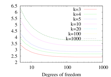
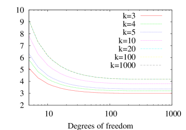
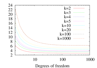
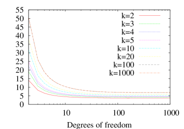
The $\chi^{2}$ distribution is obtained from the implementation in the Python “SciPy” library for all confidence levels. The SMM and SR distributions, however, are not available in any existing code library, and cannot be computed from a closed form algebraic expression. Accordingly, rather than attempt to invert a complex expression with the corresponding numerical pitfalls, we use an interpolation for these two distributions, based on tables from Rohlf and Sokal, 1981.

In both cases, the available tables are for $\mathcal{C}=95\%\text{ and }99\%$, and indexed in sample size $k$ and degrees of freedom $d$. Since the distributions are asymptotic for large $k$ and $d$, we use harmonic interpolation in each direction, i.e. in one dimension for a function $f(x)$ with $x$ lying between anchor points $x_{\_}1$ and $x_{\_}2$,

$$f(x)\sim\left[(1-a)\frac{1}{f(x_{\_}1)}+a\frac{1}{f(x_{\_}2)}\right]^{-1}$$ (9)

where $a=(x-x_{\_}1)/(x_{\_}2-x_{\_}1)$. In two dimensions we need to compute extra pseudo-anchor points. For $k_{\_}1\geq k\geq k_{\_}2$ and $d_{\_}1\geq d\geq d_{\_}2$, we can first interpolate in $k$ twice to get the new anchors $f(k,d_{\_}1)$ and $f(k,d_{\_}2)$, then interpolate between these in $d$ to obtain $f(k,d)$. Or we could swap the order, so that $f(k_{\_}1,d)$ and $f(k_{\_}2,d)$ are the intermediate points. As it happens, the order is unimportant, yielding

$$f(k,d)\sim\left[\frac{(1-a_{\_}k)(1-a_{\_}d)}{f(k_{\_}1,d_{\_}1)}+\frac{(1-a_{\_}k)\,a_{\_}d}{f(k_{\_}1,d_{\_}2)}+\frac{a_{\_}k(1-a_{\_}d)}{f(k_{\_}2,d_{\_}1)}+\frac{a_{\_}k\,a_{\_}d}{f(k_{\_}2,d_{\_}2)}+\right]^{-1}$$ (10)

where $a_{\_}k$ and $a_{\_}d$ are defined as for $a$ in equation (9), with $x$ replaced by $k$ or $d$ as appropriate.

The final implementation detail is the treatment of boundaries. The tables available to us contained $k\in[3,20]$ and $d\in[5,\infty]$ for the SMM, and $k\in[2,100]$, $d\in[1,\infty]$ for SR. As the distributions diverge for low $k$ and $d$ values, we do not attempt to “plug the gaps” at the low ends, but the asymptotic behaviour at high $k$ means that it is acceptable to lock the value at that of the last anchor points. Hence, $\text{SR}(k=200,d=4.5)$ ($d^{\,\text{SR}}=\nu^{\star}$ is not usually an integer) will actually be treated as $\text{SR}(k=100,d=4.5)$, with negligible error.

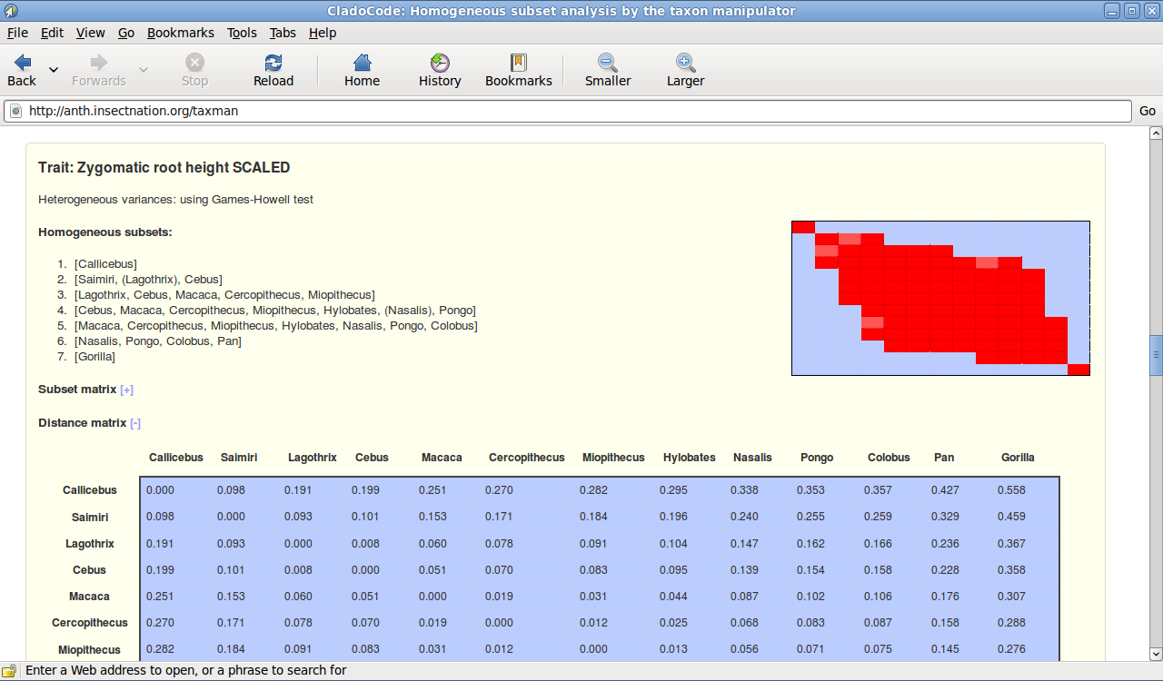
As these distributions are not to our knowledge coded in any other programs or code libraries, we have provided small programs in the TaxMan distribution which can be used to obtain harmonic interpolations automatically. These may be useful outside the context of TaxMan. The distributions themselves are plotted against $d$ for various values of $k$ in Figures 5 and 6.

Figure 5: Studentised maximum modulus distributions for confidence levels of 95% and 99% respectively

Figure 6: Studentised range distributions for confidence levels of 95% and 99% respectively

B.3 Subset identification

Identification of the subsets from the binary distance matrix, including handling of exceptional set members, is performed as described in paragraph 7 of Appendix A. However, since the procedure is relatively complex, we include here a specific implementation in pseudo-code:

highestindex $:=S$
for $i$ in $\{1\ldots S\}$:
xxx $H_{\_}i:=[\ ]$
xxx foundmatch := False
xxx highindex := 0
xxx Count backwards until a match is found, then look for exceptions
xxx for $j$ in $\{S\ldots i\}$:
xxxxxx if foundmatch = False and $\mathcal{D}_{\_}{ij}=1$:
xxxxxxxxx highindex := $j$
xxxxxxxxx foundmatch := True
xxxxxx if foundmatch:
xxxxxxxxx add $j$ to $H_{\_}i$
xxxxxx if $\mathcal{D}_{\_}{ij}=0$ and (foundmatch or $j\leq$ highestindex):
xxxxxxxxx mark $j$ as an exceptional $H_{\_}i$ member
xxxxxxxxx $\mathcal{D}_{\_}{ij}:=\mathcal{D}_{\_}{ji}:=*$

xxx Removing degenerate subsets
xxx if highindex $\leq$ highestindex:
xxxxxx discard $H_{\_}i$
xxx else:
xxxxxx highestindex := highindex

B.4 Subset and species coding scheme

We now consider the implementation of a concrete coding scheme. As described, there are two stages: the assignment of per trait subset codes and the combination of these into an overall species code.

The trait code is a case where it is tempting to think that a binary code will work well, since a binary digit can be used per subset, which is “0” if a taxon is not in the subset, and “1” if it is. However, this quickly leads to large codes, since 10 subsets gives a code with 10 binary symbols: concatenating such codes is unwieldy, even with conversion to base 10. A sequential numbering scheme is more efficient, allowing single-character representations of subsets in typical datasets. Sequential code numbers can be assigned using a simple algorithm, such as the following:

highestindex $:=S$
for $s$ in $\{1\ldots S\}$:
xxx $H_{\_}s:=[\ ]$; $C_{\_}s:=[\ ]$
for $t$ in $\{1\ldots T\}$:
xxx code = -1
xxx membership $:=[\ ]$
xxx for $s$ in $\{1\ldots S\}$:
xxxxxx prevmembership := membership
xxxxxx membership $:=[\ ]$
xxxxxx for $h$ in $\{1\ldots N_{\_}{\text{sets}}\}$:
xxxxxxxxx if $s$ is in $H_{\_}h$:
xxxxxxxxxxxx add setnum to membership
xxxxxx if membership is not prevmembership:
xxxxxxxxx code := code + 1
xxxxxx append code to $C_{\_}s$

Having generated an ordered list of code numbers for each taxon, we convert this list to a one-character-per-trait symbolic representation. We use an extension of decimal digits to alphabetic characters, as for hexadecimal, such that every code number maps to a single character in the 62-element list $[0,1,2,\dots,9,\text{a},\text{b},\dots,\text{A},\text{B},\dots]$, so that, e.g. character #18 = “h”. Each taxon’s code list is thus converted into a character string of length $T$, which is presented to the user at the end of processing. Any user who wishes to program an extension to TaxMan will have the full code objects available, rather than the string representation since the latter is fundamentally just a presentation detail.

References

- [1] Belfiore, N., Liu, L., Moritz, C. 2008. Multilocus phylogenetics of a rapid radiation in the genus Thomomys (Rodentia : Geomyidae). Syst. Biol. 57, 294–310.
- [2] Chappill, J. 1989. Quantitative characters in phylogenetic analysis. Cladistics 5, 217–234.
- [3] Collard, M., Wood, B. 2000. How reliable are human phylogenetic hypotheses? Proc. Natl. Acad. Sci. USA 97, 5003–5006.
- [4] Crisp, M., Weston, P. 1987. Cladistics and legume systematics, with an analysis of the Bossiaeeae, Brongniartieae and Mirbelieae. In: Stirton, C. (Ed.) Advances in legume systematics, part 3. Royal Botanical Gardens, Kew, pp. 65–130.
- [5] Farris, J. 1983. The logical basis of phylogenetic analysis. In: Platnick, N., Funk, V. (Eds.), Advances in cladistics, vol. 2. Columbia Univ. Press, New York, pp. 7–36.
- [6] Farris, J. 1990. Phenetics in camouflage. Cladistics 6, 91–100.
- [7] Garcia-Cruz, J., Sosa, V. 2006. Coding quantitative character data for phylogenetic analysis: a comparison of five methods. Syst. Bot. 31, 302–309.
- [8] Gilbert, C. C., Rossie, J. B. 2007. Congruence of molecules and morphology using a narrow allometric approach. Proc. Natl. Acad. Sci. USA 104, 11910–11914.
- [9] Goloboff, P. A., Farris, J. S., Nixon, K. C. 2003. T.N.T.: Tree Analysis Using New Technology. program and documentation, available from the authors, and at http://www.zmuc.dk/public/phylogeny.
- [10] Goloboff, P. A., Farris, J. S., Nixon, K. C. 2008. TNT, a free program for phylogenetic analysis. Cladistics 24, 774–786.
- [11] Goloboff, P. A., Mattoni, C. I., Quinteros, A. S. 2004. Continuous characters analyzed as such. Cladistics 20, 595–595.
- [12] Harrison, T. 1982. Small-bodied apes from the Miocene of East Africa. Ph.D. thesis, University College, London.
- [13] Higgins, D., Thompson, J., Gibson, T., Thompson, J., Higgins, D., Gibson, T. 1994. CLUSTAL W: improving the sensitivity of progressive multiple sequence alignment through sequence weighting, position-specific gap penalties and weight matrix choice. Nucleic Acids Research 22, 4673–4680.
- [14] Jungers, W. 1985. Size and scaling in primate biology. Plenum, New York.
- [15] Jungers, W., Falsetti, A., Wall, C. 1995. Shape, relative size, and size-adjustments in morphometrics. Yearb. Phys. Anthropol. 38, 137–161.
- [16] Mickevich, M., Farris, J. 1981. The implications of congruence in Menidia. Syst. Zool. 30, 351–370.
- [17] Pimentel, R., Riggins, R. 1987. The nature of cladistic data. Cladistics 3, 201–209.
- [18] Pogue, M., Mickevich, M. 1990. Character definitions and character state delineation: the bête noire of phylogenetic inference. Cladistics 6, 319–361.
- [19] Rae, T. 1993. Phylogenetic analysis of proconsulid facial morphology. Ph.D. thesis, S.U.N.Y. at Stony Brook.
- [20] Rae, T. 1997. The early evolution of the hominoid face. In: Begun, D., Ward, C., Rose, M. (Eds.), Function, phylogeny, and fossils: Miocene hominoid evolution and adaptations. Plenum, New York, pp. 59–77.
- [21] Rae, T. 1998. The logical basis for the use of continuous characters in phylogenetic systematics. Cladistics 14, 221–228.
- [22] Rae, T. 1999. Mosaic evolution in the origin of the Hominoidea. Folia Primatol. 70, 125–135.
- [23] Rae, T. 2002. Scaling, polymorphism, and cladistic analysis. In: Forey, P., MacLeod, N. (Eds.), Morphology, Shape & Phylogenetics. Taylor & Francis, London, pp. 45–52.
- [24] Rohlf, F.J., Sokal, R.R. 1981. Statistical Tables. 2nd ed. W.F. Freeman, New York.
- [25] Schols, P., Dhondt, C., Geuten, K., Merckx, V., Janssens, S., Smets, E. 2004. MorphoCode: coding quantitative data for phylogenetic analysis. Phyloinfomatics 1, 4–4.
- [26] Sharkey, M., Leathers, J. 2001. Majority does not rule: the trouble with majority-rule consensus trees. Cladistics 17, 282–284.
- [27] Simon, C. 1983. A new coding procedure for morphometric data with an example from periodical cicada wing veins. In: Felsenstein, J. (Ed.) Numerical taxonomy. Springer-Verlag, Berlin, pp. 378–382.
- [28] Slowinski, J., Corhter, B. 1998. Is the PTP test useful? Cladistics 14, 297–302.
- [29] Sokal, R., Rohlf, F. 1981. Biometry. Second edition. W.H. Freeman, New York.
- [30] Stevens, P. 1991. Character states, morphological variation, and phylogenetic analysis: a review. Syst. Bot. 16, 553–583.
- [31] Strait, D., Moniz, M., Strait, P. 1996. Finite mixture coding: a new approach to coding continuous characters. Syst. Biol. 45, 67–78.
- [32] Swiderski, D. L., Zeldich, M. L., Fink, W. L. 1998. Why morphometrics is not special: coding quantitative data for phylogenetic analysis. Syst. Biol. 47, 508–519.
- [33] Swofford, D. 2003. PAUP*. Phylogenetic Analysis Using Parsimony (*and Other Methods). Sinauer Associates, Sunderland, Massachusetts.
- [34] Thiele, K. 1993. The Holy Grail of the perfect character: the cladistic treatment of morphometric data. Cladistics 9, 275–304.
- [35] Thiele, K., Ladiges, P. 1988. A cladisitic analysis of Angophora cav. (Myrtaceae). Cladistics 4, 23–42.
- [36] Torres-Carvajal, O. 2007. Phylogeny and biogeography of a large radiation of Andean lizards (Iguania, Stenocercus). Zool. Scripta 36, 311–326.