Angular Power Spectra with Finite Counts

SheldonΒ S.Β Campbell
Center for Cosmology and AstroParticle Physics (CCAPP) and Department of Physics, The Ohio State University
191 W. Woodruff Ave., Columbus, OH 43210
(In original form 2014 October 23)
Abstract

Angular anisotropy techniques for cosmic diffuse radiation maps are powerful probes, even for quite small data sets. A popular observable is the angular power spectrum; we present a detailed study applicable to any unbinned source skymap S​(𝐧)𝑆𝐧S(\mathbf{n}) from which N𝑁N random, independent events are observed. Its exact variance, which is due to the finite statistics, depends only on S​(𝐧)𝑆𝐧S(\mathbf{n}) and N𝑁N; we also derive an unbiased estimator of the variance from the data. First-order effects agree with previous analytic estimates. Importantly, heretofore unidentified higher-order effects are found to contribute to the variance and may cause the uncertainty to be significantly larger than previous analytic estimatesβ€”potentially orders of magnitude larger. Neglect of these higher-order terms, when significant, may result in a spurious detection of the power spectrum. On the other hand, this would indicate the presence of higher-order spatial correlations, such as a large bispectrum, providing new clues about the sources. Numerical simulations are shown to support these conclusions. Applying the formalism to an ensemble of Gaussian-distributed skymaps, the noise-dominated part of the power spectrum uncertainty is significantly increased at high multipoles by the new, higher-order effects. This work is important for harmonic analyses of the distributions of diffuse high-energy γ𝛾\gamma-rays, neutrinos, and charged cosmic rays, as well as for populations of sparse point sources such as active galactic nuclei.

keywords:
methods: data analysis – methods: statistical – methods: analytical – cosmology: diffuse radiation – gamma-rays: diffuse background – neutrinos.

1 Introduction

An important experiment in astronomy is measuring the angular distribution of points on the sky from the arrival directions of incident radiation. When distance information for sources is unavailable (or too unreliable), then techniques for quantifying their two-dimensional angular distribution become essential. These methods are important for analyzing distributions of point sources, as well as incident radiation from diffuse sources (or those that appear to be, due to insufficient angular resolution).

The information contained in angular distributions depends on the application. Temperature anisotropies of the cosmic microwave background (CMB) contains information about primordial fluctuations at the epoch of last-scattering, as well as the distribution of matter and ionized gas at subsequent epochs that affected the propagation of the microwaves (e.g., WMAP Collaboration, 2013; Planck Collaboration, 2014). The distribution of galaxies (e.g., Hayes, Brunner, & Ross, 2012; Ho et al., 2012) or quasars (Leistedt et al., 2013; Ho et al., 2013) probes the large scale structure of matter. High-energy messengers, the focus of this article, have special challenges: charged cosmic rays are deflected, γ𝛾\gamma-rays can be attenuated, and neutrinos are detected only in small numbers. Directional detection of these messengers allows inferences about their sources and propagation effects.

One popular measure of the angular distribution is its power spectrum Cβ„“subscript𝐢ℓC_{\ell}, the mean-square-amplitudes of fluctuations with wavelength Ο€/β„“πœ‹β„“\pi/\ell radians, specified with a basis of spherical harmonics Yβ„“msuperscriptsubscriptπ‘Œβ„“π‘šY_{\ell}^{\,m}. These are particularly convenient observables because they characterize the angular scales of anisotropy and they are statistically orthogonal, ⟨Cℓ​Cβ„“β€²βŸ©βˆ’βŸ¨Cβ„“βŸ©β€‹βŸ¨Cβ„“β€²βŸ©βˆΞ΄β„“β€‹β„“β€²proportional-todelimited-⟨⟩subscript𝐢ℓsubscript𝐢superscriptβ„“β€²delimited-⟨⟩subscript𝐢ℓdelimited-⟨⟩subscript𝐢superscriptβ„“β€²subscript𝛿ℓsuperscriptβ„“β€²\left\langle C_{\ell}C_{\ell^{\prime}}\right\rangle-\left\langle C_{\ell}\right\rangle\left\langle C_{\ell^{\prime}}\right\rangle\propto\delta_{\ell\ell^{\prime}}, for full-sky Gaussian-distributed skymaps. Since the Cβ„“subscript𝐢ℓC_{\ell} are 2-point functions, they represent the lowest order deviations from isotropy. Such harmonic analyses are also applied to the clustering of three-dimensional cosmological data in thin spherical shells to simplify redshift distortion effects (e.g., Fisher, Schar, & Lahav, 1994; Percival et al., 2004).

One intent for analyses of galaxy surveys is to determine the statistical properties of the large scale structure in terms of their typical spatial correlations. These correlations contain information about the physics of the early Universe, the expansion history of the Universe, and the gravitational collapse of matter.

Rather than measure the statistical properties of the spatial distribution, the intent of this paper is to focus on the particular spatial distribution of observations at our particular position in the Universe we live in. We treat the power spectrum as an observable property of the source skymap itself, instead of a measurement of its statistical properties. One reason to do this is because it provides potentially important information: as the number of detected events increases, the power spectrum of high-energy gamma-rays and neutrinos will converge precisely to the flux power spectrum of their sources. In general, harmonic decompositions are a convenient way to express information about the spatial structure of astrophysical observations.

A crucial step in extracting the information contained in these measurements is assessing their uncertainty. In general, the statistical variance must be determined from the data itself.

In some cases, one can determine the variance directly from the mean or from other measurements, due to theoretical considerations. One important example is the variance of the primordial CMB temperature power spectrum, which is strongly constrained to be Gaussian-distributed, is measured with incredibly large photon counts, and where the goal is to constrain cosmological parameters. In this case, the limiting statistical uncertainty of the power spectrum is the cosmic variance over the ensemble of Universes with the same cosmology and different initial conditions. Proportional to Cβ„“2superscriptsubscript𝐢ℓ2C_{\ell}^{2}, this uncertainty is estimated with the theoretical power spectrum that best fits the data. If we didn’t have a cosmological theory of the CMB (but still knew it to be Gaussian-distributed), then the cosmic variance would need to be approximated from an estimate of Cβ„“2superscriptsubscript𝐢ℓ2C_{\ell}^{2} using the data alone. When determining the statistical uncertainty from the data in this way, one must ensure there is enough data to guarantee that the power spectrum’s error estimate is sufficiently precise.

If one wants to know the CMB power spectrum in our specific sky, perhaps to compare with the power spectrum of another related distribution such as known X-ray galaxies, its statistical uncertainty is smaller than the cosmic variance, and the limiting uncertainty is instrument noise.

Error analyses that require spatial modelling of the data (such as assuming Gaussianity, for example) may not be applicable or be easy to properly apply to data that is not well understood. There are many examples of this. The sources of ultra-high energy cosmic rays are unknown and their propagation has uncertainties that make modeling the expected signal difficult. As such, quantifying the statistical significance of observed features, such as hotspots (Telescope Array Collaboration, 2014), or dipole phase transitions (e.g., Giaccari, 2013; Ivanov et al., 2014), require a spatial-model independent approach (such as in Linsley, 1975). Likewise for anisotropy features in high-energy astrophysical ensembles of observed charged cosmic rays (e.g., Westerhoff, 2013; Santander, 2013; Desiati, 2014; Tamburro, 2014), neutrinos (IceCube Collaboration, 2013, 2014a, 2014b, 2014c), and diffuse γ𝛾\gamma-rays (Fermi-LAT Collaboration, 2012). Spatial-model independent approaches are also useful for verifying the applicability of more efficient model-dependent techniques, and providing a fall-back standard to apply in regimes where those models prove inadequate. A current example of such a modeling challenge is non-Gaussianities in the galaxy distribution induced at small distance scales (including the baryon acoustic oscillation scale) by non-linear gravitational collapse (e.g., SDSS Collaboration, 2006; Harnois-DΓ©raps & Pen, 2013).

Thus, there is a need for statistical uncertainty estimates of the power spectrum using data alone, independent of information about the radiation’s source. In particular, there has been less development of power spectrum measurements for experiments with a relatively small number of counts. Such experiments do not require data compression techniques to be appliedβ€”the low counts of high energy data may allow exact methods to be computationally tractable, without the need to bin the data into sky-pixels. For these experiments, new techniques are now needed, including methods to determine the variance of observables such as the power spectrum.

A first precise formulation of this kind is presented in this paper for the angular power spectrum of finite counts. The statistical framework is minimal and widely applicable, containing only two postulates:

  1. 1.

    stationarityβ€”the data consists of point events on a sphere sourced from a stationary skymap distribution S​(𝐧)𝑆𝐧S(\mathbf{n}), and

  2. 2.

    independenceβ€”each observed event is statistically independent of the other events (Poisson process), with its spatial probability density function proportional to S𝑆S.

The stationarity postulate is only broken when the data contains significant contributions from transients on time scales of the order of the experiment livetime. The independence postulate is broken for any beams that exhibit quantum boson bunching (such as for the CMB) or fermion antibunching (as expected in the cosmic neutrino background), known as the HBT effect (Hanbury Brown & Twiss, 1957; Zmuidzinas, 2003; Jeltes et al., 2007). Such effects are left for future studies.

With this framework, we show how to estimate the power spectrum without bias111It is worth pointing out that the presented estimators in this work are unbiased with respect to a fixed number of observed events, instead of a fixed exposure. Indeed, it is unclear how to determine an unbiased estimator of power spectrum from fixed exposure as long as there is a finite probability of receiving less than two events, in which case the estimate of the power spectrum is undefined. for any finite set of data with at least two events, and show how its variance depends on the source distribution. In particular, we find new contributions to the statistical variance of the power spectrum, due to the source distribution’s power spectrum, bispectrum, and trispectrum. We provide new unbiased estimates of the variance derived from the data, applicable for any distribution of sources. This work is immediately important for the high-energy γ𝛾\gamma-ray anisotropy analyses carried out with Fermi-LAT data (Fermi-LAT Collaboration, 2012).

For simplicity of presentation in this first paper, the analysis is presented for uniform-exposure full-sky observations.

The rest of this paper is organized as follows. In Sec.Β 2, we briefly discuss some of the current methods of power spectrum estimation, review previous analytic uncertainty estimates of the power spectrum and preview the new results of this paper for comparison. Sec.Β 3 contains the detailed derivation of the new results. Arguments are given for the specific case of a γ𝛾\gamma-ray analysis. In Sec.Β 4, we present a detailed discussion of the results, and verify the new effects in some initial numerical simulations. A discussion for the applicability of the results to other experiments appears in Sec.Β 5. We conclude in Sec.Β 6.

The error analysis of Cβ„“subscript𝐢ℓC_{\ell} is most easily expressed in terms of rotation-invariant spherical tensors of higher order than the angular power spectrum. A study of these new higher order spectra is provided in App.Β A. Despite many searches, we are unaware of any previous description of these tensors. The maximum likelihood analysis of the angular power spectrum of a Gaussian distribution on a sphere is reviewed in App.Β B, and the derivation of central moments of Gaussian fields is reviewed in App.Β C.

Some notations consistently appear in this paper. An unbiased estimator X^^𝑋\hat{X}, dependent on random data, of some physical quantity X𝑋X is denoted with a β€˜^^absent\hat{\ \ }’. Measurements of spherical-mean-normalized angular distributions are indicated throughout with a β€˜~~absent\tilde{\ \ }’.

2 Angular Power Spectra: From High to Low Statistics, From Sky Ensembles to a Single Sky

This section will briefly discuss the existing methods for power spectrum estimation, and preview the main results of this paper for comparison. The derivation of these results and detailed comparison with the existing methods are then carried out in the next section.

We will see that the current methods are suitable when data sets are very large, such as for galaxy surveys, where the goal is to ascertain the statistical correlations of the spatial distribution of the observations. Galaxy surveys are often analyzed to measure the parameters of a pre-stated cosmological model. As such, the power spectrum measurements in this context are estimators for the cosmic mean angular spectrum over an ensemble of skies that are realizations of the same distribution (i.e. produced by the fiducial cosmology). Because, of course, the experiments are limited to sample only the single sky they have access to, the analysis can never reach a statistical precision better than the cosmic variance of the measurement over the theoretical ensemble of possible skies. This cosmic variance represents a fundamental statistical limit to the precision that cosmological parameters can be determined for a given cosmological model.

In contrast, detection of high-energy cosmic radiation (such as γ𝛾\gamma-rays) have motivations of determining the sources of the radiation and learning about the high-energy processes that govern the Universe. Until a model of sources is established, experiments benefit by first focusing on measurements of the radiation distribution for our specific sky. In this context, the precision of these measurements is not bounded by cosmic variance; in fact, the distribution of a static sky can, in principle, be measured to any statistical precision, bounded only by the sky transience and irreducible experimental systematics. Matching the angular distribution of diffuse γ𝛾\gamma-rays to the distribution of potential sources is an important technique for resolving the γ𝛾\gamma-ray sky.

The additional precision achieved by measuring the power spectrum of the actual sky (rather than a cosmic mean power spectrum) is useful for searches of energy modulation features in the power spectrum from dark matter annihilation (Siegal-Gaskins & Pavlidou, 2009). Not only is the power spectrum of dark matter annihilation predicted to be significantly different from other γ𝛾\gamma-ray sources (Ando & Komatsu, 2006; Ando et al., 2007), but it is sensitive to the abundance and profile of dark matter subhalos (Campbell & Beacom, 2013; Calore et al., 2014), as well as the velocity-dependence of extragalactic annihilations (Campbell, Dutta, & Komatsu, 2010; Campbell & Dutta, 2011).

Now that the Fermi-LAT has determined a diffuse component to the cosmic γ𝛾\gamma-rays and measured a positive power spectrum, this information is already being used to constrain models of the sources (e.g., Fermi-LAT Collaboration, 2012; Cuoco, Komatsu, & Siegal-Gaskins, 2012; Harding & Abazajian, 2012; GΓ³mez-Vargas et al., 2013; Ando & Komatsu, 2013; Broderick et al., 2013b; Calore, Di Mauro, & Donato, 2014; Di Mauro et al., 2014). For example, blazars that are relatively sparse in the sky would generate a large intensity anisotropy if they were too bright, thus limiting their possible contribution to the net diffuse background (Harding & Abazajian, 2012).

This pioneering work by the Fermi-LAT collaboration had the foresight to estimate the uncertainty of the power spectrum using methods similar to the cosmological experimentsβ€”these correctly estimated the primary sources of uncertainty. The strategy applied by the Fermi-LAT working group was to analyze the earliest data set with the assumption that it is Gaussian-distributed, and to test these assumptions with subsequent data (Komatsu, private communication).

However, we will see that neglected higher order terms due to finite count effects and non-Gaussianities can produce non-negligible contributions to the variance of the power spectrum, and can be determined reliably from the data, allowing the assumption of Gaussianity to be tested immediately. Neglecting the higher order terms can cause the power spectrum variance to be biased, though whether the bias is positive or negative depends on the properties of the skymap.

It was pointed out in Broderick et al. (2013a) that the power spectrum in the highest energy bin 10.4Β GeV<E<50.0Β GeVtimes10.4GeV𝐸times50.0GeV$10.4\text{\,}\mathrm{G}\mathrm{e}\mathrm{V}$<E<$50.0\text{\,}\mathrm{G}\mathrm{e}\mathrm{V}$ was measured to be inconsistently small because subsequent resolved point sources that were not masked in the original analysis appear to produce a larger intensity power spectrum than the original measurement (an estimated 3ΟƒπœŽ\sigma discrepancy). This could indicate that the uncertainty in that energy bin was underestimated. Significant non-Gaussianities in the distribution of that energy bin would resolve this apparent discrepancy.

We now review the error analysis that is appropriate for the cosmological experiments measuring the statistics of large scale structure and formed the basis for the Fermi-LAT analysis. We then compare this technique to the new exact methods derived in this paper for measuring the power spectrum of our particular sky, which we will preview in this section without derivation. The results reveal the conditions under which the original analysis applies. A full derivation is presented in Sec.Β 3, and the consequences for inferencing the power spectrum known to be sourced from a Gaussian sky is discussed in Sec.Β 3.5.

Perhaps the most famous angular power spectrum is of the temperature fluctuations of the CMB. The Gaussianity of these fluctuations implies that their statistical properties are fully specified by their power spectrum. The method of estimating the power spectrum of the temperature field T​(𝐧)𝑇𝐧T(\mathbf{n}) via the harmonic amplitudes

cℓ​m=∫d𝐧​Yℓ​mβˆ—β€‹(𝐧)​[T​(𝐧)βˆ’T0],subscriptπ‘β„“π‘šdifferential-d𝐧subscriptsuperscriptπ‘Œβ„“π‘šπ§delimited-[]𝑇𝐧subscript𝑇0c_{\ell m}=\int\mathrm{d}\mathbf{n}\,Y^{*}_{\ell m}(\mathbf{n})\left[T(\mathbf{n})-T_{0}\right], (1)

where T0subscript𝑇0T_{0} is the mean CMB temperature, is often called the pseudo-spectrum in the CMB literature (Hivon et al., 2002)

Cβ„“=12​ℓ+1β€‹βˆ‘m=βˆ’β„“β„“|cℓ​m|2=𝒩ℓ+C^β„“.subscript𝐢ℓ12β„“1superscriptsubscriptπ‘šβ„“β„“superscriptsubscriptπ‘β„“π‘š2subscript𝒩ℓsubscript^𝐢ℓC_{\ell}=\frac{1}{2\ell+1}\sum_{m=-\ell}^{\ell}\left|c_{\ell m}\right|^{2}=\mathscr{N}_{\ell}+\hat{C}_{\ell}. (2)

The pseudo-spectrum estimator is biased by photon shot noise, sky pixelation noise, and instrument noise with spectrum 𝒩ℓsubscript𝒩ℓ\mathscr{N}_{\ell}, which is modeled and subtracted to determine the unbiased estimator C^β„“subscript^𝐢ℓ\hat{C}_{\ell} of the CMB power spectrum. For example, the instrument noise experienced by the High Frequency Instrument on the Planck Satellite is due to its bolometers’ detector noise (designed to be smaller than the photon noise produced from the cosmic background), thermal emission from the cooled telescope, and also from the cryogenic filter stages in the telescope (Holmes et al., 2008; Planck Collaboration, 2014).

While early CMB experiments made use of the pseudo-spectrum estimator, realistic implementations of the pseudo-spectrum analysis must also consider effects due to sky pixelation, masking, non-uniform exposure, and instrument resolution (Hivon et al., 2002). Computational limitations require the sky to be pixelized as an effective way to reduce the large volume of data without loss of information (Tegmark, 1997; Tegmark, Taylor, & Heavens, 1997). Modern analyses tend to also use more general quadratic maximum likelihood estimator methods on large data sets, which can be made more computationally feasible (Tegmark, 1997) and more precise for certain applications (Molinari et al., 2014). Hybrid methods also exist (Efstathiou, 2004; HAWC Collaboration, 2014). Maximum likelihood estimators generally assume the data are spatially Gaussian-distributed in order to write down a likelihood function.

It may be possible to generalize maximum-likelihood methods for non-Gaussian skymaps. In principle, it is possible to derive the probability density function (PDF) of any estimator of Cβ„“subscript𝐢ℓC_{\ell} for any set of random event data of size N𝑁N from either a fixed skymap S​(𝐧)𝑆𝐧S(\mathbf{n}) or statistical ensemble of skymaps. This PDF can then be used to determine the likelihood function for the actual value for Cβ„“subscript𝐢ℓC_{\ell}, given a particular set of data, from which the maximum likelihood estimator and minimum variance estimate can be made. The dependence on S​(𝐧)𝑆𝐧S(\mathbf{n}), though, requires careful theoretical modeling of the skymap. When a reliable model of the skymap is unavailable, methods that do not use prior information about the spatial distribution of the skymap may be more desirable. Such a method is what is presented in this paper.

When the power spectrum of fluctuations is produced by a Gaussian random process, it will differ between different realizations of the random process. When Cβ„“subscript𝐢ℓC_{\ell}, derived with Eqn.Β (2), is interpreted as an estimator of the cosmic mean power spectrum over all possible realizations of the Gaussian process, then the variance of Cβ„“subscript𝐢ℓC_{\ell} from realization to realization, i.e., the cosmic variance, is given by (see App.Β B)

𝒱​ar​[Cβ„“]=22​ℓ+1​Cβ„“2,𝒱ardelimited-[]subscript𝐢ℓ22β„“1superscriptsubscript𝐢ℓ2\mathscr{V}\!\!\text{\it ar}\,[C_{\ell}]=\frac{2}{2\ell+1}C_{\ell}^{2}, (3)

explained in App.Β B to be minimal for the estimator in Eqn.Β (2). Likewise, the variance of noise contributing to multipole β„“β„“\ell is

𝒱​ar​[𝒩ℓ]=22​ℓ+1​𝒩ℓ2.𝒱ardelimited-[]subscript𝒩ℓ22β„“1superscriptsubscript𝒩ℓ2\mathscr{V}\!\!\text{\it ar}\,[\mathscr{N}_{\ell}]=\frac{2}{2\ell+1}\mathscr{N}_{\ell}^{2}. (4)

It was demonstrated in Knox (1995) that if Gaussian fluctuations are pixelized, the determination of Cβ„“subscript𝐢ℓC_{\ell} contains a pixel noise due to fluctuation correlations within a single pixel, and then the estimator Cβ„“^^subscript𝐢ℓ\hat{C_{\ell}} is Ο‡2​ℓ+12subscriptsuperscriptπœ’22β„“1\chi^{2}_{2\ell+1} distributed with cosmic variance

𝒱​ar​[C^β„“]=22​ℓ+1​(𝒩ℓ+Cβ„“)2.𝒱ardelimited-[]subscript^𝐢ℓ22β„“1superscriptsubscript𝒩ℓsubscript𝐢ℓ2\mathscr{V}\!\!\text{\it ar}\,[\hat{C}_{\ell}]=\frac{2}{2\ell+1}\left(\mathscr{N}_{\ell}+C_{\ell}\right)^{2}. (5)

That is, it is a fundamental property of the statistical distribution of Cβ„“subscript𝐢ℓC_{\ell} that the standard deviations of Cβ„“subscript𝐢ℓC_{\ell} and 𝒩ℓsubscript𝒩ℓ\mathscr{N}_{\ell} are added to each other, not the variances (see also App.Β B for justification). This simple prescription, properly applied, was shown to give a precise characterization of the variance of Boomerang CMB data (Hivon et al., 2002). We refer to this prescription as cosmic variance with noise.

The WMAP measurement of the CMB temperature power spectrum was presented with this uncertainty separated into two contributions (WMAP Collaboration, 2013). The measured values of C^β„“subscript^𝐢ℓ\hat{C}_{\ell} had an uncertainty due to those terms containing the noise,

𝒱​ar​[C^β„“]=22​ℓ+1​𝒩ℓ​(𝒩ℓ+2​(Cth)β„“),𝒱ardelimited-[]subscript^𝐢ℓ22β„“1subscript𝒩ℓsubscript𝒩ℓ2subscriptsubscript𝐢thβ„“\mathscr{V}\!\!\text{\it ar}\,[\hat{C}_{\ell}]=\frac{2}{2\ell+1}\mathscr{N}_{\ell}\left(\mathscr{N}_{\ell}+2(C_{\text{th}})_{\ell}\right), (6)

with appropriate adjustments for binning in multipole and partial sky coverage, and where (Cth)β„“subscriptsubscript𝐢thβ„“(C_{\text{th}})_{\ell} is the best-fit theoretical power spectrum from a ΛΛ\LambdaCDM cosmology. For reasons that will become apparent, we refer to this variance as Cβ„“subscript𝐢ℓC_{\ell}-only. It represents the statistical uncertainty of the measurement, accounting for differences of the measurement from the actual power spectrum of the sky due to randomness in the data. The remaining contribution is simply the cosmic variance. It gives the magnitude that the power spectrum of our sky’s realization of the CMB fluctuations can randomly differ from the theoretical cosmic mean power spectrum. It is shown as an uncertainty band on (Cth)β„“subscriptsubscript𝐢thβ„“(C_{\text{th}})_{\ell}, representing its status as a theoretical uncertainty.

The success of this analytic variance to capture so well the simulated variances of CMB experiments motivated the use of Eqn.Β (5) in the error estimate for an early measurement of the angular power spectrum of the diffuse gamma-ray background by the Fermi-LAT collaboration (Fermi-LAT Collaboration, 2012). In this application, the noise 𝒩ℓsubscript𝒩ℓ\mathscr{N}_{\ell} corresponds to multipole-independent photon shot noise, which is the variance of the power spectrum for a Poisson point process where events are equally likely from each position in the sky. This approach was suitable for early γ𝛾\gamma-ray data sets for which the uncertainty is dominated by the shot noise. Since the shot noise term is well understood and was estimated to dominate the error bar, inaccuracies in the signal contribution to the variance were not a source of concern. Since the diffuse background appears isotropic on large angular scales, it was presumed to be dominantly from extragalactic sources. Thus, cosmic variance was included in the error estimate to aid the constraint of theoretical models of extragalactic sources on linear distance scales; however, its contribution to the error bars was negligible in that analysis.

The main goal of this paper is to carry out a detailed analytic study of the statistical uncertainty of measurements of angular power spectra derived from a finite number of independent random events, where the probability of each individual event observation is weighted according to the source’s intrinsic skymap. We focus on the case where the observed events are high-energy γ𝛾\gamma-rays, with probability weighted by the apparent flux skymap of sources with intensity power spectrum Cβ„“subscript𝐢ℓC_{\ell}. Application to other experiments is discussed in Sec.Β 5. We also focus in this paper on the measurement on our particular sky-realization’s power spectrum, for which there is no cosmic variance. In Sec.Β 3.5, we will show how to apply our results to the case of measuring the cosmic mean power spectrum of a Gaussian distribution, for which cosmic variance is an important effect.

The photon shot noise has magnitude (see Sec.Β 3.1)

𝒩=4​π​NΞ΅2𝒩4πœ‹π‘superscriptπœ€2\mathscr{N}=\frac{4\pi N}{\varepsilon^{2}} (7)

after N𝑁N γ𝛾\gamma-rays are observed over the full sky with uniform exposure Ξ΅πœ€\varepsilon. Then Eqn.Β (2) predicts that the unbiased estimator C^β„“,Nsubscript^𝐢ℓ𝑁\hat{C}_{\ell,N} of the power spectrum of the signal source is related to the power spectrum Cβ„“,Nsubscript𝐢ℓ𝑁C_{\ell,N} of the N𝑁N observed events by

Cβ„“,N=4​π​NΞ΅2+C^β„“,N.subscript𝐢ℓ𝑁4πœ‹π‘superscriptπœ€2subscript^𝐢ℓ𝑁C_{\ell,N}=\frac{4\pi N}{\varepsilon^{2}}+\hat{C}_{\ell,N}. (8)

In contrast, our analysis finds that Eqn.Β (2) is modified at low counts to

Cβ„“,N=4​π​NΞ΅2+(1βˆ’1N)​C^β„“,Nsubscript𝐢ℓ𝑁4πœ‹π‘superscriptπœ€211𝑁subscript^𝐢ℓ𝑁\boxed{C_{\ell,N}=\frac{4\pi N}{\varepsilon^{2}}+\left(1-\frac{1}{N}\right)\hat{C}_{\ell,N}} (9)

and we find that C^β„“,Nsubscript^𝐢ℓ𝑁\hat{C}_{\ell,N} can be determined directly as a sum of Legendre polynomials of the β€˜distances’ between events

C^β„“,N=4​π​N2Ξ΅2​[1N​(Nβˆ’1)β€‹βˆ‘i=1Nβˆ‘j=1jβ‰ iNPℓ​(𝐧i⋅𝐧j)βˆ’Ξ΄β„“,0].subscript^𝐢ℓ𝑁4πœ‹superscript𝑁2superscriptπœ€2delimited-[]1𝑁𝑁1superscriptsubscript𝑖1𝑁superscriptsubscript𝑗1𝑗𝑖𝑁subscript𝑃ℓ⋅subscript𝐧𝑖subscript𝐧𝑗subscript𝛿ℓ0\hat{C}_{\ell,N}=\frac{4\pi N^{2}}{\varepsilon^{2}}\Bigg{[}\frac{1}{N(N-1)}\sum_{i=1}^{N}\sum_{\begin{subarray}{c}j=1\\ j\neq i\end{subarray}}^{N}P_{\ell}(\mathbf{n}_{i}\cdot\mathbf{n}_{j})-\delta_{\ell,0}\Bigg{]}. (10)

As usual, the inner product 𝐧1⋅𝐧2β‹…subscript𝐧1subscript𝐧2\mathbf{n}_{1}\cdot\mathbf{n}_{2} is defined as the cosine of the angular distance between the positions. While this modification does not affect previous estimates of the power spectrum when N≫1much-greater-than𝑁1N\gg 1, the corrections to the measurement’s variance are potentially more important.

The variance estimate that provided the starting point for Fermi-LAT’s error analysis is the cosmic variance with shot noise variance from Eqn.Β (5),

[𝒱​ar​[C^β„“,N]]CV=22​ℓ+1​(4​π​NΞ΅2+Cβ„“)2,subscriptdelimited-[]𝒱ardelimited-[]subscript^𝐢ℓ𝑁CV22β„“1superscript4πœ‹π‘superscriptπœ€2subscript𝐢ℓ2\Big{[}\mathscr{V}\!\!\text{\it ar}\,[\hat{C}_{\ell,N}]\Big{]}_{\text{CV}}=\frac{2}{2\ell+1}\left(\frac{4\pi N}{\varepsilon^{2}}+C_{\ell}\right)^{\!\!2}, (11)

in terms of the true power spectrum Cβ„“subscript𝐢ℓC_{\ell}. The strategy to estimate this variance is to substitute Cβ„“subscript𝐢ℓC_{\ell} either with the measured spectrum C^β„“,Nsubscript^𝐢ℓ𝑁\hat{C}_{\ell,N}, or with a modeled spectrum that best fits the data. Since, as we just explained, the measurement of our particular sky does not contain cosmic variance, we remove the cosmic variance for our analysis, as in Eqn.Β (6). Thus, the analytic estimate leaves us with the Cβ„“subscript𝐢ℓC_{\ell}-only variance

𝒱​ar^​[C^β„“,N]=22​ℓ+1​4​π​NΞ΅2​(4​π​NΞ΅2+2​C^β„“,N).^𝒱ardelimited-[]subscript^𝐢ℓ𝑁22β„“14πœ‹π‘superscriptπœ€24πœ‹π‘superscriptπœ€22subscript^𝐢ℓ𝑁\widehat{\mathscr{V}\!\!\text{\it ar}}\,[\hat{C}_{\ell,N}]=\frac{2}{2\ell+1}\frac{4\pi N}{\varepsilon^{2}}\left(\frac{4\pi N}{\varepsilon^{2}}+2\hat{C}_{\ell,N}\right). (12)

Our analysis finds that the exact variance of C^β„“,Nsubscript^𝐢ℓ𝑁\hat{C}_{\ell,N} is 𝒱​ar​[C^β„“,N]𝒱ardelimited-[]subscript^𝐢ℓ𝑁\displaystyle\mathscr{V}\!\!\text{\it ar}\,[\hat{C}_{\ell,N}] =11βˆ’1N[22​ℓ+1(4​π​NΞ΅2)2\displaystyle=\frac{1}{1-\frac{1}{N}}\Bigg{[}\!\frac{2}{2\ell+1}\left(\frac{4\pi N}{\varepsilon^{2}}\right)^{\!\!2} (13) +42​ℓ+1​4​π​(Nβˆ’2)Ξ΅2​Cβ„“+32​π2Ξ΅2​Cβ„“(2)42β„“14πœ‹π‘2superscriptπœ€2subscript𝐢ℓ32superscriptπœ‹2superscriptπœ€2superscriptsubscript𝐢ℓ2\displaystyle\quad+\frac{4}{2\ell+1}\frac{4\pi(N-2)}{\varepsilon^{2}}C_{\ell}+\frac{32\pi^{2}}{\varepsilon^{2}}\,C_{\ell}^{(2)} +(1βˆ’2N)16​πΡCβ„“(3)βˆ’4​Nβˆ’6N2Cβ„“2],\displaystyle\quad+\left(1-\frac{2}{N}\right)\frac{16\pi}{\varepsilon}\,C_{\ell}^{(3)}-\frac{4N-6}{N^{2}}\,C_{\ell}^{2}\Bigg{]}, where Cβ„“(2)superscriptsubscript𝐢ℓ2C_{\ell}^{(2)} is a new 2-point spectrum that can be written as a linear combination of components of Cβ„“subscript𝐢ℓC_{\ell}, and Cβ„“(3)superscriptsubscript𝐢ℓ3C_{\ell}^{(3)} is a new 3-point spectrum that is a linear combination of components of the angular bispectrum (see App.Β A for definitions and details).

The first two terms of Eqn.Β (13) are slight corrections of Eqn.Β (12). The remaining three terms of Eqn.Β (13) are new corrections to the statistical variance of the power spectrum. Cβ„“(2)superscriptsubscript𝐢ℓ2C_{\ell}^{(2)} provides a correction to the shot noise term of the spectrum (at Nβˆ’2superscript𝑁2N^{-2}), and contributes a dependence on the power spectrum’s neighboring β„“β„“\ell components. Cβ„“(3)superscriptsubscript𝐢ℓ3C_{\ell}^{(3)} enters at the same order as the signal term (asymptotically Nβˆ’1superscript𝑁1N^{-1}), accounting for effects from the signal’s bispectrum. The Cβ„“2superscriptsubscript𝐢ℓ2C_{\ell}^{2} term provides trispectrum effects that appear to reduce both the shot and signal terms of the variance. This reduction of the power spectrum variance by the presence of a significant trispectrum is not clearly understood.

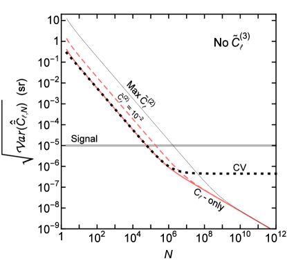
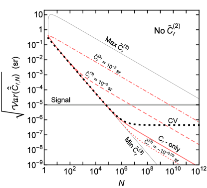
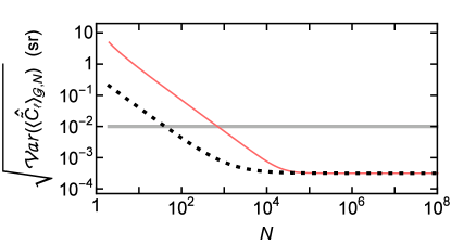
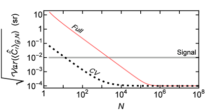
The effects of the new terms in the variance are shown in Fig.Β 1 in terms of the fluctuation power spectrum C~ℓ≑(Ξ΅/N)2​Cβ„“subscript~𝐢ℓsuperscriptπœ€π‘2subscript𝐢ℓ\tilde{C}_{\ell}\equiv(\varepsilon/N)^{2}C_{\ell} for varying magnitudes of C~β„“(2)≑(Ξ΅/N)2​Cβ„“(2)superscriptsubscript~𝐢ℓ2superscriptπœ€π‘2superscriptsubscript𝐢ℓ2\tilde{C}_{\ell}^{(2)}\equiv(\varepsilon/N)^{2}C_{\ell}^{(2)} and C~β„“(3)≑(Ξ΅/N)3​Cβ„“(3)superscriptsubscript~𝐢ℓ3superscriptπœ€π‘3superscriptsubscript𝐢ℓ3\tilde{C}_{\ell}^{(3)}\equiv(\varepsilon/N)^{3}C_{\ell}^{(3)}. For comparison, the cosmic variance with noise is also shown. A complete discussion of these effects is in Sec.Β 4.1.

Refer to caption
(a)
Refer to caption
(b)
Figure 1: Statistical uncertainty of the power spectrum of N𝑁N points at β„“=500β„“500\ell=500 when C~500=10βˆ’5Β srtimessubscript~𝐢500superscript105sr\tilde{C}_{500}=10^{-5}\text{\,}\mathrm{s}\mathrm{r}. The magnitude of C~500subscript~𝐢500\tilde{C}_{500} is indicated by the horizontal gray band. The red solid line shows the β€˜Cβ„“subscript𝐢ℓC_{\ell}-only’ variance, when the new effects from C~β„“(2)superscriptsubscript~𝐢ℓ2\tilde{C}_{\ell}^{(2)} and C~β„“(3)superscriptsubscript~𝐢ℓ3\tilde{C}_{\ell}^{(3)} are negligible. For comparison, the cosmic variance with noise scenarioβ€”which is used for probing extragalactic source modelsβ€”is shown with the black dotted curve labelled β€˜CV’. Left: The effect of a non-negligible C~β„“(2)superscriptsubscript~𝐢ℓ2\tilde{C}_{\ell}^{(2)} increases the shot-dominated portion of the uncertainty, as shown by the dashed red curve, though never enough to reach the β€˜max’ thin black line. Right: A significant positive bispectrum produces an early signal transition (red dashed curve) slowing the rate at which the uncertainty decreases with additional counts. This produces a much larger statistical error. The dot-dashed curve shows the effect for a very large C~β„“(3)superscriptsubscript~𝐢ℓ3\tilde{C}_{\ell}^{(3)}, becoming up to 1000 times larger than the Cβ„“subscript𝐢ℓC_{\ell}-only error, and showing that it may be possible for the signal term to always exceed the shot term. The signal term cannot be as large as the β€˜max’ thin black line. A negative bispectrum is possible (red dotted curve), and is the only way for this variance to be significantly below the Cβ„“subscript𝐢ℓC_{\ell}-only estimate for this small value of C~β„“subscript~𝐢ℓ\tilde{C}_{\ell}, though not below the β€˜min’ thin black line. For comparison, the Fermi-LAT analysis measured a similar power spectrum with N∼105βˆ’106similar-to𝑁superscript105superscript106N\sim 10^{5}-10^{6} events per energy bin over ∼1/3similar-toabsent13\sim 1/3 of the sky (Fermi-LAT Collaboration, 2012). See Sec.Β 4.1 for a complete discussion of these results.

In addition, we derived an unbiased estimator for the variance from the N𝑁N data points, presented in Sec.Β 3.4. Importantly, it allows the uncertainty to be estimated from the data, independent of any simulations or assumed models of the sources. There are simple estimators for the shot term and signal term separately, but their sum simplifies further to the total estimator

𝒱​ar^​[C^β„“,N]=C^β„“,N2βˆ’C^β„“,N(4)^𝒱ardelimited-[]subscript^𝐢ℓ𝑁superscriptsubscript^𝐢ℓ𝑁2superscriptsubscript^𝐢ℓ𝑁4\boxed{\widehat{\mathscr{V}\!\!\text{\it ar}}\,[\hat{C}_{\ell,N}]=\hat{C}_{\ell,N}^{2}-\hat{C}_{\ell,N}^{(4)}} (14)

using Eqn.Β (10) and the estimator of the trispectrum term

C^β„“,N(4)=(4​π​N2Ξ΅2)2[1N​(Nβˆ’1)​(Nβˆ’2)​(Nβˆ’3)βˆ‘i1βˆ‘i2β‰ i1\displaystyle\hat{C}_{\ell,N}^{(4)}=\!\left(\!\frac{4\pi N^{2}}{\varepsilon^{2}}\!\right)^{\!\!2}\Bigg{[}\frac{1}{N(N-1)(N-2)(N-3)}\sum_{i_{1}}\sum_{i_{2}\neq i_{1}}
βˆ‘i3βˆ‰{i1,i2}βˆ‘i4βˆ‰{i1,i2,i3}Pβ„“(𝐧1⋅𝐧2)Pβ„“(𝐧3⋅𝐧4)βˆ’Ξ΄β„“,0].\displaystyle\!\!\!\!\!\!\!\!\!\!\sum_{\ \ \ \ \ i_{3}\notin\{i_{1},i_{2}\}}\!\!\!\!\!\!\!\!\!\!\!\!\sum_{\ \ \ \ \ \ \ i_{4}\notin\{i_{1},i_{2},i_{3}\}}P_{\ell}(\mathbf{n}_{1}\cdot\mathbf{n}_{2})P_{\ell}(\mathbf{n}_{3}\cdot\mathbf{n}_{4})-\delta_{\ell,0}\Bigg{]}. (15)

The simplicity of Eqns.Β (10) and (14) suggest that it is practical for sufficiently small counts to consider the events point-by-point as opposed to binned in pixels. This would have the additional benefit of not having to account for artificial pixel effects in the results.

The complete derivation of all these results is carried out in the following section.

3 Angular Power Spectra of Cosmic Events

The new error analysis technique is now described. The problem statement for this analysis can be given in a general way. In this section, we will apply it specifically to high-energy γ𝛾\gamma-ray events, and will briefly discuss other experiments in Sec.Β 5.

A position on the sky (i.e. on a sphere) is given by a unit vector 𝐧𝐧\mathbf{n} pointing from the sphere’s center. If a spherical coordinate system is defined on the sphere, then 𝐧=(ΞΈ,Ο•)π§πœƒitalic-Ο•\mathbf{n}=(\theta,\phi) may be specified by polar angle ΞΈπœƒ\theta and azimuthal angle Ο•italic-Ο•\phi.

We identify a class of events to be analyzed, and identify their positions in the sky 𝐧1,𝐧2,𝐧3,…subscript𝐧1subscript𝐧2subscript𝐧3…\mathbf{n}_{1},\mathbf{n}_{2},\mathbf{n}_{3},\ldots . For the case of γ𝛾\gamma-ray events, these could be a particular class of event reconstruction in some specified energy range.

Let S​(𝐧)𝑆𝐧S(\mathbf{n}) be the actual angular distribution of the signal’s intrinsic β€˜skymap’: the rate of events at each position, as would be observed in the limit of infinite N𝑁N. For γ𝛾\gamma-rays, S​(𝐧)𝑆𝐧S(\mathbf{n}) is the apparent γ𝛾\gamma-ray flux over the energy range of interest.

Note that no effects due to the instrument’s point spread function (PSF) are being applied to S​(𝐧)𝑆𝐧S(\mathbf{n}). However, we will explicitly derive in Sec.Β 3.2 that the only effect of the PSF is to convolve with S​(𝐧)𝑆𝐧S(\mathbf{n}), and that the measured spectrum is an estimator of the convolved skymap. We will thereafter assume that S​(𝐧)𝑆𝐧S(\mathbf{n}) refers to the intrinsic skymap convolved with the instrument PSF.

If S​(𝐧)𝑆𝐧S(\mathbf{n}) is non-negative and non-trivial (i.e., not zero everywhere), then a very useful quantity is the normalized skymap

S~​(𝐧)≑S​(𝐧)∫d​𝐧′4​π​S​(𝐧′),~𝑆𝐧𝑆𝐧dsuperscript𝐧′4πœ‹π‘†superscript𝐧′\tilde{S}(\mathbf{n})\equiv\frac{S(\mathbf{n})}{\int{\frac{\mathrm{d}\mathbf{n}^{\prime}}{4\pi}}\,S(\mathbf{n}^{\prime})}, (16)

which fluctuates around 1 on the sphere. Note that d​𝐧=d​ϕ​d​(cos⁑θ)d𝐧ditalic-Ο•dπœƒ\mathrm{d}\mathbf{n}=\mathrm{d}\phi\,\mathrm{d}(\cos\theta) denotes the usual sphere measure.

The power spectrum and fluctuation power spectrum of the skymap are

Cβ„“=12​ℓ+1β€‹βˆ‘m=βˆ’β„“β„“|cℓ​m|2,subscript𝐢ℓ12β„“1superscriptsubscriptπ‘šβ„“β„“superscriptsubscriptπ‘β„“π‘š2\displaystyle C_{\ell}=\frac{1}{2\ell+1}\sum_{m=-\ell}^{\ell}\left|c_{\ell m}\right|^{2}, (17)
C~β„“=12​ℓ+1β€‹βˆ‘m=βˆ’β„“β„“|c~ℓ​m|2,subscript~𝐢ℓ12β„“1superscriptsubscriptπ‘šβ„“β„“superscriptsubscript~π‘β„“π‘š2\displaystyle\tilde{C}_{\ell}=\frac{1}{2\ell+1}\sum_{m=-\ell}^{\ell}\left|\tilde{c}_{\ell m}\right|^{2}, (18)

where cℓ​msubscriptπ‘β„“π‘šc_{\ell m} is the spherical transform of Sβˆ’βˆ«S​d𝐧/(4​π)𝑆𝑆differential-d𝐧4πœ‹S-\int{S\,\mathrm{d}\mathbf{n}/(4\pi)}, and c~ℓ​msubscript~π‘β„“π‘š\tilde{c}_{\ell m} is the spherical transform of S~βˆ’1~𝑆1\tilde{S}-1. The values of cℓ​msubscriptπ‘β„“π‘šc_{\ell m} are not invariant under rotations of the sphere and depend on the definition of the spherical coordinate system applied to the sphere, but Cβ„“subscript𝐢ℓC_{\ell} is a rotation-invariant tensor.

The problem is to consider N𝑁N points received from random locations on the sphere with probability distribution specified by S~​(𝐧)~𝑆𝐧\tilde{S}(\mathbf{n}), and determine the mean and variance of the power spectrum of these events.

For the observation of radiation events, it is useful to determine the intensity power spectrum. Let π’œβ€‹(𝐧,t)π’œπ§π‘‘\mathcal{A}(\mathbf{n},t) be the effective area of the instrument to events from position 𝐧𝐧\mathbf{n} at time t𝑑t. Then the total exposure of the instrument is

Ρ​(t)=∫dπ§β€‹βˆ«0tdtβ€²β€‹π’œβ€‹(𝐧,tβ€²)πœ€π‘‘differential-d𝐧superscriptsubscript0𝑑differential-dsuperscriptπ‘‘β€²π’œπ§superscript𝑑′\varepsilon(t)=\int{\mathrm{d}\mathbf{n}}\int_{0}^{t}{\mathrm{d}t^{\prime}}\,\mathcal{A}(\mathbf{n},t^{\prime}) (19)

integrated over the field of observation in the sky, and instrument livetime. Let N​(t)𝑁𝑑N(t) be the number of detected events with this exposure. Then the total observed intensity is

I​(𝐧,t)=d​N​(𝐧,t)d​Ω​dβ€‹π’œβ€‹d​t=4​πΡ​(t)β€‹βˆ‘i=1N​(t)wi​(t)​δ​(π§βˆ’π§i),𝐼𝐧𝑑d𝑁𝐧𝑑dΞ©dπ’œd𝑑4πœ‹πœ€π‘‘superscriptsubscript𝑖1𝑁𝑑subscript𝑀𝑖𝑑𝛿𝐧subscript𝐧𝑖I(\mathbf{n},t)=\frac{\mathrm{d}N(\mathbf{n},t)}{\mathrm{d}\Omega\,\mathrm{d}\mathcal{A}\,\mathrm{d}t}=\frac{4\pi}{\varepsilon(t)}\sum_{i=1}^{N(t)}w_{i}(t)\,\delta(\mathbf{n}-\mathbf{n}_{i}), (20)

where ΩΩ\Omega is the solid angle of observation, and

wi​(t)≑Ρ​(t)4β€‹Ο€β€‹βˆ«0tdtβ€²β€‹π’œβ€‹(𝐧i,tβ€²)subscriptπ‘€π‘–π‘‘πœ€π‘‘4πœ‹superscriptsubscript0𝑑differential-dsuperscriptπ‘‘β€²π’œsubscript𝐧𝑖superscript𝑑′w_{i}(t)\equiv\frac{\varepsilon(t)}{4\pi\int_{0}^{t}\mathrm{d}t^{\prime}\,\mathcal{A}(\mathbf{n}_{i},t^{\prime})} (21)

is the exposure weighting for event i𝑖i.

The work in this paper will restrict to the simple experiment where the full sky is being observed with uniform exposure. In this case, wi=1subscript𝑀𝑖1w_{i}=1 for all events. These results can be generalized in future work to account for partial sky coverage with a non-uniform exposure map.

Denote cℓ​m,Nsubscriptπ‘β„“π‘šπ‘c_{\ell m,N} as the central spherical transform of the intensity from N𝑁N events

cℓ​m,Nsubscriptπ‘β„“π‘šπ‘\displaystyle c_{\ell m,N} =∫d𝐧​Yℓ​mβˆ—β€‹(𝐧)​[I​(𝐧)βˆ’βˆ«d​𝐧′4​π​I​(𝐧′)]absentdifferential-d𝐧subscriptsuperscriptπ‘Œβ„“π‘šπ§delimited-[]𝐼𝐧dsuperscript𝐧′4πœ‹πΌsuperscript𝐧′\displaystyle=\int\mathrm{d}\mathbf{n}\,Y^{*}_{\ell m}(\mathbf{n})\left[I(\mathbf{n})-\int\frac{\mathrm{d}\mathbf{n}^{\prime}}{4\pi}I(\mathbf{n}^{\prime})\right]
=4β€‹Ο€Ξ΅β€‹βˆ‘i=1NYℓ​mβˆ—β€‹(𝐧i)βˆ’4​π​NΡ​δℓ,0​δm,0,absent4πœ‹πœ€superscriptsubscript𝑖1𝑁subscriptsuperscriptπ‘Œβ„“π‘šsubscript𝐧𝑖4πœ‹π‘πœ€subscript𝛿ℓ0subscriptπ›Ώπ‘š0\displaystyle=\frac{4\pi}{\varepsilon}\sum_{i=1}^{N}Y^{*}_{\ell m}(\mathbf{n}_{i})-\frac{\sqrt{4\pi}\,N}{\varepsilon}\delta_{\ell,0}\delta_{m,0}, (22)

with the intensity power spectrum of the detected events being

Cβ„“,N=12​ℓ+1β€‹βˆ‘m=βˆ’β„“β„“|cℓ​m,N|2.subscript𝐢ℓ𝑁12β„“1superscriptsubscriptπ‘šβ„“β„“superscriptsubscriptπ‘β„“π‘šπ‘2C_{\ell,N}=\frac{1}{2\ell+1}\sum_{m=-\ell}^{\ell}\left|c_{\ell m,N}\right|^{2}. (23)

A useful alternative expression for the power spectrum can be found by using the spherical harmonic addition theorem in Eqn.Β (143),

Cβ„“,N=4​πΡ2β€‹βˆ‘i=1Nβˆ‘j=1NPℓ​(𝐧i⋅𝐧j)βˆ’4​π​N2Ξ΅2​δℓ,0.subscript𝐢ℓ𝑁4πœ‹superscriptπœ€2superscriptsubscript𝑖1𝑁superscriptsubscript𝑗1𝑁subscript𝑃ℓ⋅subscript𝐧𝑖subscript𝐧𝑗4πœ‹superscript𝑁2superscriptπœ€2subscript𝛿ℓ0C_{\ell,N}=\frac{4\pi}{\varepsilon^{2}}\sum_{i=1}^{N}\sum_{j=1}^{N}P_{\ell}(\mathbf{n}_{i}\cdot\mathbf{n}_{j})-\frac{4\pi N^{2}}{\varepsilon^{2}}\delta_{\ell,0}. (24)

The fluctuation power spectrum, which also applies to counts of celestial objects, is found by normalizing the spherical transform by the mean intensity N/Ξ΅π‘πœ€N/\varepsilon:

c~ℓ​m,N​(𝐧1,…,𝐧N)=4​πNβ€‹βˆ‘i=1NYℓ​mβˆ—β€‹(𝐧i)βˆ’4​π​δℓ,0​δm,0,subscript~π‘β„“π‘šπ‘subscript𝐧1…subscript𝐧𝑁4πœ‹π‘superscriptsubscript𝑖1𝑁subscriptsuperscriptπ‘Œβ„“π‘šsubscript𝐧𝑖4πœ‹subscript𝛿ℓ0subscriptπ›Ώπ‘š0\displaystyle\tilde{c}_{\ell m,N}(\mathbf{n}_{1},\ldots,\mathbf{n}_{N})=\frac{4\pi}{N}\sum_{i=1}^{N}Y^{*}_{\ell m}(\mathbf{n}_{i})-\sqrt{4\pi}\delta_{\ell,0}\delta_{m,0}, (25)
C~β„“,N​(𝐧1,…,𝐧N)=4​πN2β€‹βˆ‘i=1Nβˆ‘j=1NPℓ​(𝐧i⋅𝐧j)βˆ’4​π​δℓ,0.subscript~𝐢ℓ𝑁subscript𝐧1…subscript𝐧𝑁4πœ‹superscript𝑁2superscriptsubscript𝑖1𝑁superscriptsubscript𝑗1𝑁subscript𝑃ℓ⋅subscript𝐧𝑖subscript𝐧𝑗4πœ‹subscript𝛿ℓ0\displaystyle\tilde{C}_{\ell,N}(\mathbf{n}_{1},\ldots,\mathbf{n}_{N})=\frac{4\pi}{N^{2}}\sum_{i=1}^{N}\sum_{j=1}^{N}P_{\ell}(\mathbf{n}_{i}\cdot\mathbf{n}_{j})-4\pi\delta_{\ell,0}. (26)

Statistical properties of these observables will now be considered. The results will be presented in terms of the fluctuation power spectrum, but can be converted to the intensity power spectrum by multiplying C~β„“subscript~𝐢ℓ\tilde{C}_{\ell} by the mean intensity squared N2/Ξ΅2superscript𝑁2superscriptπœ€2N^{2}/\varepsilon^{2}.

In the limit that the uncertainty in Ξ΅πœ€\varepsilon is negligible, the use of Cβ„“subscript𝐢ℓC_{\ell} or C~β„“subscript~𝐢ℓ\tilde{C}_{\ell} are equivalent. Since the fluctuation spectra are independent of Ξ΅πœ€\varepsilon, they are not affected by any systematics present in the estimate of the exposure.

3.1 Shot Noise and Point Spread: Angular Power Spectrum of Events from an Isotropic Sky

The analysis is begun by considering the case of an isotropic skymap, such that S~​(𝐧)=1~𝑆𝐧1\tilde{S}(\mathbf{n})=1. This is both instructive as a review of results for a Poisson point process, and useful by providing some necessary intermediate formulae involving the effect of an instrument’s PSF.

Define the point spread function as F​(𝐧s,𝐧)𝐹subscript𝐧𝑠𝐧F(\mathbf{n}_{s},\mathbf{n}) as the probability density function (PDF) of observing (or reconstructing) an event at 𝐧𝐧\mathbf{n} given that it was sourced from position 𝐧ssubscript𝐧𝑠\mathbf{n}_{s}. In general, this function can depend on other parameters that categorize the events and can affect the angular precision of observation. As a PDF, F𝐹F is normalized over all possible reconstruction positions such that

∫d​𝐧4​π​F​(𝐧s,𝐧)=1.d𝐧4πœ‹πΉsubscript𝐧𝑠𝐧1\int\frac{\mathrm{d}\mathbf{n}}{4\pi}F(\mathbf{n}_{s},\mathbf{n})=1. (27)

Let ψ=cosβˆ’1⁑(𝐧s⋅𝐧)πœ“superscript1β‹…subscript𝐧𝑠𝐧\psi=\cos^{-1}(\mathbf{n}_{s}\cdot\mathbf{n}) be the angle of misreconstruction. If the PSF angular dependence is isotropic (depending on Οˆπœ“\psi alone), then it is a symmetric PSF with F​(𝐧s,𝐧)=F​(𝐧,𝐧s)𝐹subscript𝐧𝑠𝐧𝐹𝐧subscript𝐧𝑠F(\mathbf{n}_{s},\mathbf{n})=F(\mathbf{n},\mathbf{n}_{s}), and it follows that F𝐹F is also normalized to 111 over the skymap positions 𝐧ssubscript𝐧𝑠\mathbf{n}_{s}. However, this need not be the case in general.

For good angular resolution, the PSF is sometimes well-described in the flat-sky limit as a Gaussian beam, often expressed as

Fflat​(ψ)=12​π​σb2​exp⁑[βˆ’Οˆ22​σb2],subscript𝐹flatπœ“12πœ‹superscriptsubscriptπœŽπ‘2superscriptπœ“22superscriptsubscriptπœŽπ‘2F_{\text{flat}}(\psi)=\frac{1}{2\pi\sigma_{b}^{2}}\exp\left[-\frac{\psi^{2}}{2\sigma_{b}^{2}}\right], (28)

with width ΟƒbsubscriptπœŽπ‘\sigma_{b} expressed in radians. One finds that the fraction f​(p)𝑓𝑝f(p) of events observed within angles ψ<p​σbπœ“π‘subscriptπœŽπ‘\psi<p\sigma_{b} is f​(p)=1βˆ’eβˆ’p2/2𝑓𝑝1superscript𝑒superscript𝑝22f(p)=1-e^{-p^{2}/2}. The fraction of events within ψ<Οƒbπœ“subscriptπœŽπ‘\psi<\sigma_{b} is f​(1)≃0.393similar-to-or-equals𝑓10.393f(1)\simeq 0.393, and the 68% containment angle (i.e., the angular radius that contains 68% of events from a point source) is ψ68≃1.51​σbsimilar-to-or-equalssubscriptπœ“681.51subscriptπœŽπ‘\psi_{68}\simeq 1.51\sigma_{b}. One simple extension of this to the sphere is the Fisher distribution (Fisher, 1953)

FF​(𝐧s,𝐧)=Οƒbβˆ’2​csch​(Οƒbβˆ’2)​exp⁑[𝐧s⋅𝐧σb2].subscript𝐹𝐹subscript𝐧𝑠𝐧superscriptsubscriptπœŽπ‘2cschsuperscriptsubscriptπœŽπ‘2β‹…subscript𝐧𝑠𝐧superscriptsubscriptπœŽπ‘2F_{F}(\mathbf{n}_{s},\mathbf{n})=\sigma_{b}^{-2}\,\text{csch}\!\left(\sigma_{b}^{-2}\right)\exp\!\left[\frac{\mathbf{n}_{s}\cdot\mathbf{n}}{\sigma_{b}^{2}}\right]. (29)

Armed with our two postulates of stationarity of S𝑆S and independence of the N𝑁N events, the determination of statistical moments of the power spectrum is divided into two parts. The first calculation is to determine, for fixed source positions 𝐧s​1,𝐧s​2,…subscript𝐧𝑠1subscript𝐧𝑠2…\mathbf{n}_{s1},\mathbf{n}_{s2},\ldots, the moment averaged over the PSF, which will be denoted with an overbar

X¯​(𝐧s​1,…,𝐧s​N)β‰‘βˆ«[∏id​𝐧i4​π​F​(𝐧s​i,𝐧i)]​X​(𝐧1,…​𝐧N).¯𝑋subscript𝐧𝑠1…subscript𝐧𝑠𝑁delimited-[]subscriptproduct𝑖dsubscript𝐧𝑖4πœ‹πΉsubscript𝐧𝑠𝑖subscript𝐧𝑖𝑋subscript𝐧1…subscript𝐧𝑁\overline{X}(\mathbf{n}_{s1},\ldots,\mathbf{n}_{sN})\equiv\int\left[\prod_{i}\frac{\mathrm{d}\mathbf{n}_{i}}{4\pi}F(\mathbf{n}_{si},\mathbf{n}_{i})\right]X(\mathbf{n}_{1},\ldots\mathbf{n}_{N}). (30)

With that result, the second step is to take an ensemble average of the N𝑁N observed event positions over the sphere, giving the full moment of the measurement denoted with angle brackets,

⟨XβŸ©β‰‘βˆ«[∏id​𝐧s​i4​π​S~​(𝐧s​i)]​X¯​(𝐧s​1,…,𝐧s​N),delimited-βŸ¨βŸ©π‘‹delimited-[]subscriptproduct𝑖dsubscript𝐧𝑠𝑖4πœ‹~𝑆subscript𝐧𝑠𝑖¯𝑋subscript𝐧𝑠1…subscript𝐧𝑠𝑁\left\langle X\right\rangle\equiv\int\left[\prod_{i}\frac{\mathrm{d}\mathbf{n}_{si}}{4\pi}\tilde{S}(\mathbf{n}_{si})\right]\overline{X}(\mathbf{n}_{s1},\ldots,\mathbf{n}_{sN}), (31)

written for an isotropic source as

⟨X⟩0β‰‘βˆ«[∏id​𝐧s​i4​π]​X¯​(𝐧s​1,…,𝐧s​N).subscriptdelimited-βŸ¨βŸ©π‘‹0delimited-[]subscriptproduct𝑖dsubscript𝐧𝑠𝑖4πœ‹Β―π‘‹subscript𝐧𝑠1…subscript𝐧𝑠𝑁\left\langle X\right\rangle_{0}\equiv\int\left[\prod_{i}\frac{\mathrm{d}\mathbf{n}_{si}}{4\pi}\right]\overline{X}(\mathbf{n}_{s1},\ldots,\mathbf{n}_{sN}). (32)

This last step in Eqn.Β (31) is where the independence postulate of the received events is applied.

Consider the spherical transform c~ℓ​m,N​(𝐧1,…,𝐧N)subscript~π‘β„“π‘šπ‘subscript𝐧1…subscript𝐧𝑁\tilde{c}_{\ell m,N}(\mathbf{n}_{1},\ldots,\mathbf{n}_{N}) of the observed events, which is an interesting property of the distribution in its own right, and consider the mean of its measurement. Let 𝐧s​isubscript𝐧𝑠𝑖\mathbf{n}_{si} be the actual skymap position of the observed/reconstructed event position 𝐧isubscript𝐧𝑖\mathbf{n}_{i}. Averaging over the PSF of each event gives

c~ℓ​m,NΒ―Β―subscript~π‘β„“π‘šπ‘\displaystyle\overline{\tilde{c}_{\ell m,N}} (𝐧s​1,…,𝐧s​N)subscript𝐧𝑠1…subscript𝐧𝑠𝑁\displaystyle(\mathbf{n}_{s1},\ldots,\mathbf{n}_{sN})
=∫[∏id​𝐧i4​π​F​(𝐧s​i,𝐧i)]​c~ℓ​m,N​(𝐧1,…,𝐧N)absentdelimited-[]subscriptproduct𝑖dsubscript𝐧𝑖4πœ‹πΉsubscript𝐧𝑠𝑖subscript𝐧𝑖subscript~π‘β„“π‘šπ‘subscript𝐧1…subscript𝐧𝑁\displaystyle=\int\left[\prod_{i}\frac{\mathrm{d}\mathbf{n}_{i}}{4\pi}F(\mathbf{n}_{si},\mathbf{n}_{i})\right]\tilde{c}_{\ell m,N}(\mathbf{n}_{1},\ldots,\mathbf{n}_{N})
=1Nβ€‹βˆ‘i=1NFℓ​m​(𝐧s​i),absent1𝑁superscriptsubscript𝑖1𝑁subscriptπΉβ„“π‘šsubscript𝐧𝑠𝑖\displaystyle=\frac{1}{N}\sum_{i=1}^{N}F_{\ell m}(\mathbf{n}_{si}), (33)

where the spherical transform of the PSF is defined as

Fℓ​m​(𝐧s)β‰‘βˆ«d𝐧​Yℓ​mβˆ—β€‹(𝐧)​[F​(𝐧s,𝐧)βˆ’1].subscriptπΉβ„“π‘šsubscript𝐧𝑠differential-d𝐧superscriptsubscriptπ‘Œβ„“π‘šπ§delimited-[]𝐹subscript𝐧𝑠𝐧1F_{\ell m}(\mathbf{n}_{s})\equiv\int\mathrm{d}\mathbf{n}\,Y_{\ell m}^{*}(\mathbf{n})\Big{[}F(\mathbf{n}_{s},\mathbf{n})-1\Big{]}. (34)

Averaging over all source positions for an isotropic skymap, a symmetric PSF produces the usual result

⟨c~ℓ​m,N⟩0=∫[∏id​𝐧s​i4​π]​c~ℓ​m,N¯​(𝐧s​1,…,𝐧s​N)=0.subscriptdelimited-⟨⟩subscript~π‘β„“π‘šπ‘0delimited-[]subscriptproduct𝑖dsubscript𝐧𝑠𝑖4πœ‹Β―subscript~π‘β„“π‘šπ‘subscript𝐧𝑠1…subscript𝐧𝑠𝑁0\left\langle\tilde{c}_{\ell m,N}\right\rangle_{0}=\int\left[\prod_{i}\frac{\mathrm{d}\mathbf{n}_{si}}{4\pi}\right]\overline{\tilde{c}_{\ell m,N}}(\mathbf{n}_{s1},\ldots,\mathbf{n}_{sN})=0. (35)

This tells us the mean of the spherical transform measurement of isotropy is 0, but does not tell us the level of statistical fluctuation we expect. To determine this variance, calculate

|c~ℓ​m,N|2Β―Β―superscriptsubscript~π‘β„“π‘šπ‘2\displaystyle\overline{\left|\tilde{c}_{\ell m,N}\right|^{2}} =4​πN(1βˆ’Ξ΄β„“,0Ξ΄m,0)+4​πN2[βˆ‘iFℓ​mm(𝐧s​i)\displaystyle=\frac{4\pi}{N}\left(1-\delta_{\ell,0}\delta_{m,0}\right)+\frac{4\pi}{N^{2}}\Bigg{[}\sum_{i}F_{\ell m}^{\ \ \,m}(\mathbf{n}_{si})
+14β€‹Ο€βˆ‘iβˆ‘jβ‰ iFℓ​m(𝐧s​i)Fβ„“m(𝐧s​j)].\displaystyle\quad+\frac{1}{4\pi}\sum_{i}\sum_{j\neq i}F_{\ell m}(\mathbf{n}_{si})F_{\ell}^{\,m}(\mathbf{n}_{sj})\Bigg{]}. (36)

This result produces a rank 2 spherical transform (see AppendixΒ A),

Fℓ​mm​(𝐧s)=∫d𝐧​|Yβ„“m​(𝐧)|2​[F​(𝐧s,𝐧)βˆ’1],superscriptsubscriptπΉβ„“π‘šπ‘šsubscript𝐧𝑠differential-d𝐧superscriptsuperscriptsubscriptπ‘Œβ„“π‘šπ§2delimited-[]𝐹subscript𝐧𝑠𝐧1F_{\ell m}^{\ \ \,m}(\mathbf{n}_{s})=\int\mathrm{d}\mathbf{n}\left|Y_{\ell}^{\,m}(\mathbf{n})\right|^{2}\Big{[}F(\mathbf{n}_{s},\mathbf{n})-1\Big{]}, (37)

from the 1-event contributions, the terms where the contribution from each factor of c~ℓ​m,Nsubscript~π‘β„“π‘šπ‘\tilde{c}_{\ell m,N} is from the same event. The other β€˜2-event’ terms generate a product of rankΒ 1 transforms. This leads for isotropic sky and symmetric PSF to a mean square of

⟨|c~ℓ​m,N|2⟩0=4​πN​(1βˆ’Ξ΄β„“,0​δm,0),subscriptdelimited-⟨⟩superscriptsubscript~π‘β„“π‘šπ‘204πœ‹π‘1subscript𝛿ℓ0subscriptπ›Ώπ‘š0\left\langle\left|\tilde{c}_{\ell m,N}\right|^{2}\right\rangle_{0}=\frac{4\pi}{N}\left(1-\delta_{\ell,0}\,\delta_{m,0}\right), (38)

which in this case is the expected variance 𝒱​ar​[c~ℓ​m,N]𝒱ardelimited-[]subscript~π‘β„“π‘šπ‘\mathscr{V}\!\!\text{\it ar}\,[\tilde{c}_{\ell m,N}]. Thus, a lack of signal produces spherical transforms of the data that randomly distribute about zero with a variance of 4​π/N4πœ‹π‘4\pi/N (for β„“>0β„“0\ell>0).

Carrying out this calculation with the power spectrum of the data produces a PSF average

C~β„“,N¯​(𝐧s​1,…,𝐧s​N)=12​ℓ+1β€‹βˆ‘m|c~ℓ​m,N|2Β―Β―subscript~𝐢ℓ𝑁subscript𝐧𝑠1…subscript𝐧𝑠𝑁12β„“1subscriptπ‘šΒ―superscriptsubscript~π‘β„“π‘šπ‘2\displaystyle\overline{\tilde{C}_{\ell,N}}(\mathbf{n}_{s1},\ldots,\mathbf{n}_{sN})=\frac{1}{2\ell+1}\sum_{m}\overline{\left|\tilde{c}_{\ell m,N}\right|^{2}}
=4​πN​(1βˆ’Ξ΄β„“,0)+1N2β€‹βˆ‘iβˆ‘jβ‰ i𝒲ℓ​(𝐧s​i,𝐧s​j),absent4πœ‹π‘1subscript𝛿ℓ01superscript𝑁2subscript𝑖subscript𝑗𝑖subscript𝒲ℓsubscript𝐧𝑠𝑖subscript𝐧𝑠𝑗\displaystyle=\frac{4\pi}{N}\left(1-\delta_{\ell,0}\right)+\frac{1}{N^{2}}\sum_{i}\sum_{j\neq i}\mathscr{W}_{\ell}(\mathbf{n}_{si},\mathbf{n}_{sj}), (39)

in terms of the power spectrum of the PSF

𝒲ℓ​(𝐧s​1,𝐧s​2)=12​ℓ+1β€‹βˆ‘mFℓ​m​(𝐧s​1)​Fβ„“m​(𝐧s​2)subscript𝒲ℓsubscript𝐧𝑠1subscript𝐧𝑠212β„“1subscriptπ‘šsubscriptπΉβ„“π‘šsubscript𝐧𝑠1superscriptsubscriptπΉβ„“π‘šsubscript𝐧𝑠2\displaystyle\mathscr{W}_{\ell}(\mathbf{n}_{s1},\mathbf{n}_{s2})=\frac{1}{2\ell+1}\sum_{m}F_{\ell m}(\mathbf{n}_{s1})F_{\ell}^{\,m}(\mathbf{n}_{s2}) (40)
=4β€‹Ο€β€‹βˆ«d​𝐧14​π​d​𝐧24​π​[F​(𝐧s​1,𝐧1)βˆ’1]​Pℓ​(𝐧1⋅𝐧2)​[F​(𝐧s​2,𝐧2)βˆ’1]absent4πœ‹dsubscript𝐧14πœ‹dsubscript𝐧24πœ‹delimited-[]𝐹subscript𝐧𝑠1subscript𝐧11subscript𝑃ℓ⋅subscript𝐧1subscript𝐧2delimited-[]𝐹subscript𝐧𝑠2subscript𝐧21\displaystyle\!\!=\!4\pi\!\!\int\!\!\frac{\mathrm{d}\mathbf{n}_{1}}{4\pi}\frac{\mathrm{d}\mathbf{n}_{2}}{4\pi}\Big{[}F(\mathbf{n}_{s1},\mathbf{n}_{1})\!-\!1\Big{]}P_{\ell}(\mathbf{n}_{1}\!\cdot\!\mathbf{n}_{2})\Big{[}F(\mathbf{n}_{s2},\mathbf{n}_{2})\!-\!1\Big{]}

If the PSF is symmetric, then it depends only on μ≑𝐧sβ‹…π§πœ‡β‹…subscript𝐧𝑠𝐧\mu\equiv\mathbf{n}_{s}\cdot\mathbf{n}, and it has a corresponding instrument window function

Wβ„“β‰‘βˆ«βˆ’11d​μ2​Pℓ​(ΞΌ)​F​(ΞΌ).subscriptπ‘Šβ„“superscriptsubscript11dπœ‡2subscriptπ‘ƒβ„“πœ‡πΉπœ‡W_{\ell}\equiv\int_{-1}^{1}\frac{\mathrm{d}\mu}{2}P_{\ell}(\mu)F(\mu). (41)

For the Fisher distribution in Eqn.Β (29),

(WF)β„“=Ο€2β€‹Οƒβˆ’1​csch​(Οƒβˆ’2)​Iβ„“+12​(Οƒβˆ’2),subscriptsubscriptπ‘ŠπΉβ„“πœ‹2superscript𝜎1cschsuperscript𝜎2subscript𝐼ℓ12superscript𝜎2(W_{F})_{\ell}=\sqrt{\frac{\pi}{2}}\sigma^{-1}\text{csch}(\sigma^{-2})I_{\ell+\frac{1}{2}}(\sigma^{-2}), (42)

where Iν​(x)subscript𝐼𝜈π‘₯I_{\nu}(x) is the Ξ½thsuperscript𝜈th\nu^{\text{th}} modified Bessel function of the first kind. When Οƒbβ‰ͺ1much-less-thansubscriptπœŽπ‘1\sigma_{b}\ll 1, this is indistinguishable from

(Wflat)β„“=eβˆ’β„“β€‹(β„“+1)​σb2/2,subscriptsubscriptπ‘Šflatβ„“superscript𝑒ℓℓ1superscriptsubscriptπœŽπ‘22(W_{\text{flat}})_{\ell}=e^{-\ell(\ell+1)\sigma_{b}^{2}/2}, (43)

which at large β„“β„“\ell is the Fourier transform of Eqn.Β (28). With the window function, the power spectrum of a symmetric PSF is

𝒲ℓ​(𝐧s​1,𝐧s​2)=4​π​Wβ„“2​[Pℓ​(𝐧s​1⋅𝐧s​2)βˆ’Ξ΄β„“,0].subscript𝒲ℓsubscript𝐧𝑠1subscript𝐧𝑠24πœ‹superscriptsubscriptπ‘Šβ„“2delimited-[]subscript𝑃ℓ⋅subscript𝐧𝑠1subscript𝐧𝑠2subscript𝛿ℓ0\mathscr{W}_{\ell}(\mathbf{n}_{s1},\mathbf{n}_{s2})=4\pi W_{\ell}^{2}\left[P_{\ell}(\mathbf{n}_{s1}\cdot\mathbf{n}_{s2})-\delta_{\ell,0}\right]. (44)

The spherical average of Eqn.Β (39) is

⟨C~β„“,N⟩0=4​πN(1βˆ’Ξ΄β„“,0).\boxed{\left\langle\tilde{C}_{\ell,N}\right\rangle_{0}=\frac{4\pi}{N}\left(1-\delta_{\ell,0}\right).} (45)

This is the usual shot noise, or Poisson noise, of angular power spectra. This average is biased from the actual value of 00 for the isotropic skymap. As is well known and will be verified in the next subsection, this shot noise also provides a statistical bias to the estimation of the power spectrum of an anisotropic skymap.

The power spectrum squared of the N𝑁N events contains a quadruple sum over the N𝑁N positions

C~β„“,N2=(4​π)2N4β€‹βˆ‘i1=1Nβˆ‘i2=1Nβˆ‘i3=1Nβˆ‘i4=1NPℓ​(𝐧i1⋅𝐧i2)​Pℓ​(𝐧i3⋅𝐧i4)superscriptsubscript~𝐢ℓ𝑁2superscript4πœ‹2superscript𝑁4superscriptsubscriptsubscript𝑖11𝑁superscriptsubscriptsubscript𝑖21𝑁superscriptsubscriptsubscript𝑖31𝑁superscriptsubscriptsubscript𝑖41𝑁subscript𝑃ℓ⋅subscript𝐧subscript𝑖1subscript𝐧subscript𝑖2subscript𝑃ℓ⋅subscript𝐧subscript𝑖3subscript𝐧subscript𝑖4\displaystyle\tilde{C}_{\ell,N}^{2}=\frac{(4\pi)^{2}}{N^{4}}\sum_{i_{1}=1}^{N}\sum_{i_{2}=1}^{N}\sum_{i_{3}=1}^{N}\sum_{i_{4}=1}^{N}P_{\ell}(\mathbf{n}_{i_{1}}\cdot\mathbf{n}_{i_{2}})P_{\ell}(\mathbf{n}_{i_{3}}\cdot\mathbf{n}_{i_{4}})
βˆ’(4​π)2​δℓ,0superscript4πœ‹2subscript𝛿ℓ0\displaystyle\qquad\qquad-(4\pi)^{2}\delta_{\ell,0} (46)
≑[C~β„“,N2]1+[C~β„“,N2]2+[C~β„“,N2]3+[C~β„“,N2]4βˆ’(4​π)2​δℓ,0,absentsubscriptdelimited-[]superscriptsubscript~𝐢ℓ𝑁21subscriptdelimited-[]superscriptsubscript~𝐢ℓ𝑁22subscriptdelimited-[]superscriptsubscript~𝐢ℓ𝑁23subscriptdelimited-[]superscriptsubscript~𝐢ℓ𝑁24superscript4πœ‹2subscript𝛿ℓ0\displaystyle\equiv\left[\tilde{C}_{\ell,N}^{2}\right]_{1}+\left[\tilde{C}_{\ell,N}^{2}\right]_{2}+\left[\tilde{C}_{\ell,N}^{2}\right]_{3}+\left[\tilde{C}_{\ell,N}^{2}\right]_{4}-(4\pi)^{2}\delta_{\ell,0},

which is convenient to separate into a 1-event term, 2-event term, and so on. The PSF mean of the 1-event term, i.e., the sum of those terms where all 4 events are the same, is

[C~β„“,N2Β―]1=(4​π)2N3.subscriptdelimited-[]Β―superscriptsubscript~𝐢ℓ𝑁21superscript4πœ‹2superscript𝑁3\left[\overline{\tilde{C}_{\ell,N}^{2}}\right]_{1}=\frac{(4\pi)^{2}}{N^{3}}. (47)

The 2-event terms are categorized by

[C~β„“,N2Β―]2=(4​π)2N4β€‹βˆ‘i1βˆ‘i2β‰ i1∫d​𝐧i14​π​d​𝐧i24​π​F​(𝐧s​i1,𝐧i1)subscriptdelimited-[]Β―superscriptsubscript~𝐢ℓ𝑁22superscript4πœ‹2superscript𝑁4subscriptsubscript𝑖1subscriptsubscript𝑖2subscript𝑖1dsubscript𝐧subscript𝑖14πœ‹dsubscript𝐧subscript𝑖24πœ‹πΉsubscript𝐧𝑠subscript𝑖1subscript𝐧subscript𝑖1\displaystyle\!\!\!\left[\overline{\tilde{C}_{\ell,N}^{2}}\right]_{2}=\frac{(4\pi)^{2}}{N^{4}}\sum_{i_{1}}\sum_{i_{2}\neq i_{1}}\int\frac{\mathrm{d}\mathbf{n}_{i_{1}}}{4\pi}\frac{\mathrm{d}\mathbf{n}_{i_{2}}}{4\pi}F(\mathbf{n}_{si_{1}},\mathbf{n}_{i_{1}})
F​(𝐧s​i2,𝐧i2)​[4​Pℓ​(𝐧i1⋅𝐧i2)+2​Pβ„“2​(𝐧i1⋅𝐧i2)+1].𝐹subscript𝐧𝑠subscript𝑖2subscript𝐧subscript𝑖2delimited-[]4subscript𝑃ℓ⋅subscript𝐧subscript𝑖1subscript𝐧subscript𝑖22superscriptsubscript𝑃ℓ2β‹…subscript𝐧subscript𝑖1subscript𝐧subscript𝑖21\displaystyle F(\mathbf{n}_{si_{2}},\mathbf{n}_{i_{2}})\Big{[}4P_{\ell}(\mathbf{n}_{i_{1}}\cdot\mathbf{n}_{i_{2}})+2P_{\ell}^{2}(\mathbf{n}_{i_{1}}\cdot\mathbf{n}_{i_{2}})+1\Big{]}. (48)

The result in the square brackets shows how the 7 ways to pair 4 position are partitioned. The 4 ways to split the events so three are the same (different from the fourth) give the first term in the square brackets. The second term, with Pβ„“2superscriptsubscript𝑃ℓ2P_{\ell}^{2}, is generated from pairings that split the azimuthal indices, i.e., with i1=i3subscript𝑖1subscript𝑖3i_{1}=i_{3} and i2=i4subscript𝑖2subscript𝑖4i_{2}=i_{4}, or i1=i4subscript𝑖1subscript𝑖4i_{1}=i_{4} and i2=i3subscript𝑖2subscript𝑖3i_{2}=i_{3}. The last term is from the pairing that respects the azimuthal indices, with i1=i2subscript𝑖1subscript𝑖2i_{1}=i_{2} and i3=i4subscript𝑖3subscript𝑖4i_{3}=i_{4}. The Legendre polynomial term generates a power spectrum of the PSF, and the square polynomial term produces a composite power spectrum of F𝐹F (see AppendixΒ A)

𝒲ℓ(2)​(𝐧s​1,𝐧s​2)superscriptsubscript𝒲ℓ2subscript𝐧𝑠1subscript𝐧𝑠2\displaystyle\mathscr{W}_{\ell}^{(2)}(\mathbf{n}_{s1},\mathbf{n}_{s2}) (49)
=∫d​𝐧14​π​d​𝐧24​π​F​(𝐧1,𝐧s​1)​Pβ„“2​(𝐧1⋅𝐧2)​F​(𝐧2,𝐧s​2)βˆ’12​ℓ+1.absentdsubscript𝐧14πœ‹dsubscript𝐧24πœ‹πΉsubscript𝐧1subscript𝐧𝑠1superscriptsubscript𝑃ℓ2β‹…subscript𝐧1subscript𝐧2𝐹subscript𝐧2subscript𝐧𝑠212β„“1\displaystyle=\!\int\!\frac{\mathrm{d}\mathbf{n}_{1}}{4\pi}\frac{\mathrm{d}\mathbf{n}_{2}}{4\pi}F(\mathbf{n}_{1},\mathbf{n}_{s1})P_{\ell}^{2}(\mathbf{n}_{1}\!\cdot\!\mathbf{n}_{2})F(\mathbf{n}_{2},\mathbf{n}_{s2})-\frac{1}{2\ell+1}.

The 2-event term is thus

[C~β„“,N2Β―]2=(4​π)2N4{βˆ‘i1βˆ‘i2β‰ i1[4(𝒲ℓ​(𝐧s​i1,𝐧s​i2)4​π+Ξ΄β„“,0)\displaystyle\left[\overline{\tilde{C}_{\ell,N}^{2}}\right]_{2}=\frac{(4\pi)^{2}}{N^{4}}\Bigg{\{}\!\sum_{i_{1}}\sum_{i_{2}\neq i_{1}}\Bigg{[}4\Bigg{(}\frac{\mathscr{W}_{\ell}(\mathbf{n}_{si_{1}},\mathbf{n}_{si_{2}})}{4\pi}+\delta_{\ell,0}\Bigg{)}
+2(𝒲ℓ(2)(𝐧s​i1,𝐧s​i2)+12​ℓ+1)]+N(Nβˆ’1)}\displaystyle\quad\ +2\Bigg{(}\mathscr{W}_{\ell}^{(2)}(\mathbf{n}_{si_{1}},\mathbf{n}_{si_{2}})+\frac{1}{2\ell+1}\Bigg{)}\Bigg{]}+N(N-1)\Bigg{\}}
=(4​π)2N4[N(Nβˆ’1)(1+22​ℓ+1+4Ξ΄β„“,0)\displaystyle=\frac{(4\pi)^{2}}{N^{4}}\Bigg{[}N(N-1)\left(1+\frac{2}{2\ell+1}+4\delta_{\ell,0}\right) (50)
+βˆ‘i1βˆ‘i2β‰ i1(4𝒲ℓ​(𝐧s​i1,𝐧s​i2)4​π+2𝒲ℓ(2)(𝐧s​i1,𝐧s​i2))]\displaystyle\quad\ +\sum_{i_{1}}\sum_{i_{2}\neq i_{1}}\Bigg{(}4\frac{\mathscr{W}_{\ell}(\mathbf{n}_{si_{1}},\mathbf{n}_{si_{2}})}{4\pi}+2\mathscr{W}_{\ell}^{(2)}(\mathbf{n}_{si_{1}},\mathbf{n}_{si_{2}})\Bigg{)}\Bigg{]}

For the 3-event terms, there are 6 ways to choose 2 of the 4 positions to be the same event

[C~β„“,N2Β―]3=(4​π)2N4β€‹βˆ‘i1βˆ‘i2β‰ i1βˆ‘i3βˆ‰{i1,i2}∫d​𝐧i14​π​d​𝐧i24​π​d​𝐧i34​πsubscriptdelimited-[]Β―superscriptsubscript~𝐢ℓ𝑁23superscript4πœ‹2superscript𝑁4subscriptsubscript𝑖1subscriptsubscript𝑖2subscript𝑖1subscriptsubscript𝑖3subscript𝑖1subscript𝑖2dsubscript𝐧subscript𝑖14πœ‹dsubscript𝐧subscript𝑖24πœ‹dsubscript𝐧subscript𝑖34πœ‹\displaystyle\left[\overline{\tilde{C}_{\ell,N}^{2}}\right]_{3}\!=\frac{(4\pi)^{2}}{N^{4}}\sum_{i_{1}}\sum_{i_{2}\neq i_{1}}\!\!\!\!\!\!\!\!\!\!\sum_{\ \ \ \ \ i_{3}\notin\{i_{1},i_{2}\}}\int\frac{\mathrm{d}\mathbf{n}_{i_{1}}}{4\pi}\frac{\mathrm{d}\mathbf{n}_{i_{2}}}{4\pi}\frac{\mathrm{d}\mathbf{n}_{i_{3}}}{4\pi}
F(𝐧s​i1,𝐧i1)F(𝐧s​i2,𝐧i2)F(𝐧s​i3,𝐧i3)[2Pβ„“(𝐧i1⋅𝐧i2)\displaystyle\qquad F(\mathbf{n}_{si_{1}},\mathbf{n}_{i_{1}})F(\mathbf{n}_{si_{2}},\mathbf{n}_{i_{2}})F(\mathbf{n}_{si_{3}},\mathbf{n}_{i_{3}})\left[2P_{\ell}(\mathbf{n}_{i_{1}}\cdot\mathbf{n}_{i_{2}})\right.
+4Pβ„“(𝐧i1⋅𝐧i2)Pβ„“(𝐧i2⋅𝐧i3)]\displaystyle\qquad+4\left.\!P_{\ell}(\mathbf{n}_{i_{1}}\cdot\mathbf{n}_{i_{2}})P_{\ell}(\mathbf{n}_{i_{2}}\cdot\mathbf{n}_{i_{3}})\right] (51)

The first term in the square brackets comes from the 2 ways to pair events with the same azimuthal index, i1=i2subscript𝑖1subscript𝑖2i_{1}=i_{2} or i3=i4subscript𝑖3subscript𝑖4i_{3}=i_{4}. The other pairings generate an open bispectrum of the PSF (see Eqn.Β (159))

𝒲ℓ(3)​(𝐧s​1,𝐧s​2,𝐧s​3)=4β€‹Ο€β€‹βˆ«d​𝐧14​π​d​𝐧24​π​d​𝐧34​πsuperscriptsubscript𝒲ℓ3subscript𝐧𝑠1subscript𝐧𝑠2subscript𝐧𝑠34πœ‹dsubscript𝐧14πœ‹dsubscript𝐧24πœ‹dsubscript𝐧34πœ‹\displaystyle\!\!\!\!\mathscr{W}_{\ell}^{(3)}(\mathbf{n}_{s1},\mathbf{n}_{s2},\mathbf{n}_{s3})=4\pi\int\frac{\mathrm{d}\mathbf{n}_{1}}{4\pi}\frac{\mathrm{d}\mathbf{n}_{2}}{4\pi}\frac{\mathrm{d}\mathbf{n}_{3}}{4\pi}
F​(𝐧s​1,𝐧1)​Pℓ​(𝐧1⋅𝐧3)​F​(𝐧s​3,𝐧3)​Pℓ​(𝐧3⋅𝐧2)​F​(𝐧s​2,𝐧2)𝐹subscript𝐧𝑠1subscript𝐧1subscript𝑃ℓ⋅subscript𝐧1subscript𝐧3𝐹subscript𝐧𝑠3subscript𝐧3subscript𝑃ℓ⋅subscript𝐧3subscript𝐧2𝐹subscript𝐧𝑠2subscript𝐧2\displaystyle F(\mathbf{n}_{s1},\mathbf{n}_{1})P_{\ell}(\mathbf{n}_{1}\cdot\mathbf{n}_{3})F(\mathbf{n}_{s3},\mathbf{n}_{3})P_{\ell}(\mathbf{n}_{3}\cdot\mathbf{n}_{2})F(\mathbf{n}_{s2},\mathbf{n}_{2})
βˆ’π’²β„“β€‹(𝐧s​1,𝐧s​2)2​ℓ+1βˆ’4​π​δℓ,0.subscript𝒲ℓsubscript𝐧𝑠1subscript𝐧𝑠22β„“14πœ‹subscript𝛿ℓ0\displaystyle-\frac{\mathscr{W}_{\ell}(\mathbf{n}_{s1},\mathbf{n}_{s2})}{2\ell+1}-4\pi\delta_{\ell,0}. (52)

Then we find that the expression

[C~β„“,N2Β―]3=(4​π)2N4{2(Nβˆ’2)βˆ‘i1βˆ‘i2β‰ i1[𝒲ℓ​(𝐧s​i1,𝐧s​i2)4​π+Ξ΄β„“,0]\displaystyle\!\!\left[\overline{\tilde{C}_{\ell,N}^{2}}\right]_{3}\!\!=\!\frac{(4\pi)^{2}}{N^{4}}\Bigg{\{}\!2(N-2)\!\sum_{i_{1}}\!\sum_{i_{2}\neq i_{1}}\!\!\Bigg{[}\!\frac{\mathscr{W}_{\ell}(\mathbf{n}_{si_{1}},\mathbf{n}_{si_{2}})}{4\pi}+\delta_{\ell,0}\!\Bigg{]}
+4βˆ‘i1βˆ‘i2β‰ i1βˆ‘i3βˆ‰{i1,i2}[𝒲ℓ(3)​(𝐧s​i1,𝐧s​i2,𝐧s​i3)4​π\displaystyle\qquad+4\sum_{i_{1}}\!\sum_{i_{2}\neq i_{1}}\!\!\!\!\!\!\!\!\!\!\sum_{\ \ \ \ \ i_{3}\notin\{i_{1},i_{2}\}}\!\!\Bigg{[}\!\frac{\mathscr{W}_{\ell}^{(3)}(\mathbf{n}_{si_{1}},\mathbf{n}_{si_{2}},\mathbf{n}_{si_{3}})}{4\pi}
+𝒲ℓ​(𝐧s​i1,𝐧s​i2)4​π​(2​ℓ+1)+Ξ΄β„“,0]}\displaystyle\qquad+\frac{\mathscr{W}_{\ell}(\mathbf{n}_{si_{1}},\mathbf{n}_{si_{2}})}{4\pi(2\ell+1)}+\delta_{\ell,0}\!\Bigg{]}\Bigg{\}}
=(4​π)2N4[6N(Nβˆ’1)(Nβˆ’2)Ξ΄β„“,0\displaystyle=\frac{(4\pi)^{2}}{N^{4}}\Bigg{[}6N(N-1)(N-2)\delta_{\ell,0} (53)
+2​(Nβˆ’2)​(1+22​ℓ+1)β€‹βˆ‘i1βˆ‘i2β‰ i1𝒲ℓ​(𝐧s​i1,𝐧s​i2)4​π2𝑁2122β„“1subscriptsubscript𝑖1subscriptsubscript𝑖2subscript𝑖1subscript𝒲ℓsubscript𝐧𝑠subscript𝑖1subscript𝐧𝑠subscript𝑖24πœ‹\displaystyle\qquad+2(N-2)\left(1+\frac{2}{2\ell+1}\right)\sum_{i_{1}}\!\sum_{i_{2}\neq i_{1}}\frac{\mathscr{W}_{\ell}(\mathbf{n}_{si_{1}},\mathbf{n}_{si_{2}})}{4\pi}
+4βˆ‘i1βˆ‘i2β‰ i1βˆ‘i3βˆ‰{i1,i2}𝒲ℓ(3)​(𝐧s​i1,𝐧s​i2,𝐧s​i3)4​π]\displaystyle\qquad+4\sum_{i_{1}}\!\sum_{i_{2}\neq i_{1}}\!\!\!\!\!\!\!\!\!\!\sum_{\ \ \ \ \ i_{3}\notin\{i_{1},i_{2}\}}\!\!\!\!\!\!\frac{\mathscr{W}_{\ell}^{(3)}(\mathbf{n}_{si_{1}},\mathbf{n}_{si_{2}},\mathbf{n}_{si_{3}})}{4\pi}\Bigg{]}

constitutes all of the 3-event contributions.

Finally, the 4-event terms are simply

[C~β„“,N2Β―]4=(4​π)2N4β€‹βˆ‘i1βˆ‘i2β‰ i1[𝒲ℓ​(𝐧s​i1,𝐧s​i2)4​π+Ξ΄β„“,0]subscriptdelimited-[]Β―superscriptsubscript~𝐢ℓ𝑁24superscript4πœ‹2superscript𝑁4subscriptsubscript𝑖1subscriptsubscript𝑖2subscript𝑖1delimited-[]subscript𝒲ℓsubscript𝐧𝑠subscript𝑖1subscript𝐧𝑠subscript𝑖24πœ‹subscript𝛿ℓ0\displaystyle\left[\overline{\tilde{C}_{\ell,N}^{2}}\right]_{4}=\frac{(4\pi)^{2}}{N^{4}}\!\sum_{i_{1}}\!\sum_{i_{2}\neq i_{1}}\Bigg{[}\frac{\mathscr{W}_{\ell}(\mathbf{n}_{si_{1}},\mathbf{n}_{si_{2}})}{4\pi}+\delta_{\ell,0}\Bigg{]}
βˆ‘i3βˆ‰{i1,i2}βˆ‘i4βˆ‰{i1,i2,i3}[𝒲ℓ​(𝐧s​i3,𝐧s​i4)4​π+Ξ΄β„“,0]subscriptsubscript𝑖3subscript𝑖1subscript𝑖2subscriptsubscript𝑖4subscript𝑖1subscript𝑖2subscript𝑖3delimited-[]subscript𝒲ℓsubscript𝐧𝑠subscript𝑖3subscript𝐧𝑠subscript𝑖44πœ‹subscript𝛿ℓ0\displaystyle\qquad\!\!\!\!\!\!\!\!\!\!\sum_{\ \ \ \ \ i_{3}\notin\{i_{1},i_{2}\}}\!\!\!\!\!\!\!\!\!\!\!\!\sum_{\ \ \ \ \ \ \ i_{4}\notin\{i_{1},i_{2},i_{3}\}}\Bigg{[}\frac{\mathscr{W}_{\ell}(\mathbf{n}_{si_{3}},\mathbf{n}_{si_{4}})}{4\pi}+\delta_{\ell,0}\Bigg{]}
=(4​π)2N4[N(Nβˆ’1)(Nβˆ’2)(Nβˆ’3)Ξ΄β„“,0\displaystyle=\frac{(4\pi)^{2}}{N^{4}}\Bigg{[}N(N-1)(N-2)(N-3)\delta_{\ell,0} (54)
+βˆ‘i1βˆ‘i2β‰ i1βˆ‘i3βˆ‰{i1,i2}βˆ‘i4βˆ‰{i1,i2,i3}𝒲ℓ​(𝐧s​i1,𝐧s​i2)4​π𝒲ℓ​(𝐧s​i3,𝐧s​i4)4​π].\displaystyle+\!\!\sum_{i_{1}}\!\!\sum_{i_{2}\neq i_{1}}\!\!\!\!\!\!\!\!\!\!\sum_{\ \ \ \ \ i_{3}\notin\{i_{1},i_{2}\}}\!\!\!\!\!\!\!\!\!\!\!\!\!\!\sum_{\ \ \ \ \ \ \ i_{4}\notin\{i_{1},i_{2},i_{3}\}}\!\!\!\!\!\!\!\!\!\!\!\!\!\!\!\frac{\mathscr{W}_{\ell}(\mathbf{n}_{si_{1}},\mathbf{n}_{si_{2}})}{4\pi}\frac{\mathscr{W}_{\ell}(\mathbf{n}_{si_{3}},\mathbf{n}_{si_{4}})}{4\pi}\!\Bigg{]}.

The combination of the terms has cancellations, leaving us with the major result

C~β„“,N2Β―=(4​π)2N4{N2[1+(1βˆ’1N)22​ℓ+1](1βˆ’Ξ΄β„“,0)\displaystyle\overline{\tilde{C}_{\ell,N}^{2}}=\frac{(4\pi)^{2}}{N^{4}}\Bigg{\{}N^{2}\left[1+\left(1-\frac{1}{N}\right)\frac{2}{2\ell+1}\right](1-\delta_{\ell,0})
+βˆ‘i1βˆ‘i2β‰ i1[2N[1+(1βˆ’2N)22​ℓ+1]𝒲ℓ​(𝐧s​i1,𝐧s​i2)4​π\displaystyle+\sum_{i_{1}}\sum_{i_{2}\neq i_{1}}\Bigg{[}2N\left[1+\left(1-\frac{2}{N}\right)\frac{2}{2\ell+1}\right]\frac{\mathscr{W}_{\ell}(\mathbf{n}_{si_{1}},\mathbf{n}_{si_{2}})}{4\pi}
+2𝒲ℓ(2)(𝐧s​i1,𝐧s​i2)+βˆ‘i3βˆ‰{i1,i2}(4𝒲ℓ(3)​(𝐧s​i1,𝐧s​i2,𝐧s​i3)4​π\displaystyle+2\mathscr{W}_{\ell}^{(2)}(\mathbf{n}_{si_{1}},\mathbf{n}_{si_{2}})+\!\!\!\!\!\!\!\!\!\!\sum_{\ \ \ \ \ i_{3}\notin\{i_{1},i_{2}\}}\!\!\Bigg{(}4\frac{\mathscr{W}_{\ell}^{(3)}(\mathbf{n}_{si_{1}},\mathbf{n}_{si_{2}},\mathbf{n}_{si_{3}})}{4\pi}
+βˆ‘i4βˆ‰{i1,i2,i3}𝒲ℓ​(𝐧s​i1​𝐧s​i2)4​π𝒲ℓ​(𝐧s​i3,𝐧s​i4)4​π)]},\displaystyle+\!\!\!\!\!\!\!\!\!\!\!\!\!\sum_{\ \ \ \ \ \ \ i_{4}\notin\{i_{1},i_{2},i_{3}\}}\!\!\!\!\frac{\mathscr{W}_{\ell}(\mathbf{n}_{si_{1}}\mathbf{n}_{si_{2}})}{4\pi}\frac{\mathscr{W}_{\ell}(\mathbf{n}_{si_{3}},\mathbf{n}_{si_{4}})}{4\pi}\Bigg{)}\Bigg{]}\Bigg{\}}, (55)

from which all other conclusions are easily derived. For instance, we have for an isotropic background that the measurement of shot noise with a symmetric PSF has second moment

⟨C~β„“,N2⟩0=(4​πN)2​[1+(1βˆ’1N)​22​ℓ+1]​(1βˆ’Ξ΄β„“,0),subscriptdelimited-⟨⟩superscriptsubscript~𝐢ℓ𝑁20superscript4πœ‹π‘2delimited-[]111𝑁22β„“11subscript𝛿ℓ0\left\langle\tilde{C}_{\ell,N}^{2}\right\rangle_{\!0}=\left(\frac{4\pi}{N}\right)^{\!\!2}\!\left[1+\left(1-\frac{1}{N}\right)\frac{2}{2\ell+1}\right](1-\delta_{\ell,0}), (56)

and the variance of shot noise is

𝒱ar[C~β„“,N]0=(4​πN)2(1βˆ’1N)22​ℓ+1(1βˆ’Ξ΄β„“,0).\boxed{\mathscr{V}\!\!\text{\it ar}\,[\tilde{C}_{\ell,N}]_{0}=\left(\frac{4\pi}{N}\right)^{\!\!2}\!\left(1-\frac{1}{N}\right)\frac{2}{2\ell+1}(1-\delta_{\ell,0}).} (57)

It is worth noting that Eqns.Β (35), (38), (45), and (57) for the moments of an isotropic sky (shot noise) are the results one gets without a PSF, with F​(𝐧s,𝐧)=1𝐹subscript𝐧𝑠𝐧1F(\mathbf{n}_{s},\mathbf{n})=1. This demonstrates that a symmetric PSF does not affect the statistical properties of measurements of the spherical transform or power spectrum of an isotropic skymap.

3.2 An Unbiased Estimator of the Source Angular Power Spectrum

Now consider an intrinsic skymap that is anisotropic with normalized distribution S~​(𝐧)~𝑆𝐧\tilde{S}(\mathbf{n}). The spectra moments must now be calculated as in Eqn.Β (31) instead of Eqn.Β (32).

When taking the position ensemble mean of a transform or spectrum of the PSF, each skymap-weighted integration that acts on the PSF has the effect of convolving the skymap over the PSF

S~F​(𝐧)=∫d​𝐧s4​π​S~​(𝐧s)​F​(𝐧s,𝐧).subscript~𝑆𝐹𝐧dsubscript𝐧𝑠4πœ‹~𝑆subscript𝐧𝑠𝐹subscript𝐧𝑠𝐧\tilde{S}_{F}(\mathbf{n})=\int\frac{\mathrm{d}\mathbf{n}_{s}}{4\pi}\tilde{S}(\mathbf{n}_{s})F(\mathbf{n}_{s},\mathbf{n}). (58)

This PSF-convolved skymap contains the information that the instrument is capable of probing. Information that is lost in the convolution is inaccessible because of the finite angular resolution of the instrument. Therefore, the power spectrum that is being probed by cosmic events is not the power spectrum of the complete skymap, but the power spectrum of the convolved skymap.

Using Eqn.Β (44), the power spectrum C~F​ℓsubscript~𝐢𝐹ℓ\tilde{C}_{F\ell} of the skymap convolved by a symmetric PSF is related to C~β„“subscript~𝐢ℓ\tilde{C}_{\ell} by

C~F​ℓ=Wβ„“2​C~β„“.subscript~𝐢𝐹ℓsuperscriptsubscriptπ‘Šβ„“2subscript~𝐢ℓ\tilde{C}_{F\ell}=W_{\ell}^{2}\tilde{C}_{\ell}. (59)

We will not de-convolve the skymap by dividing out the window function, but will express results more simply in terms of the directly-observed PSF-convolved skymap.

For the rest of this article, it will be implicitly understood that the spherical transforms c~ℓ​msubscript~π‘β„“π‘š\tilde{c}_{\ell m} and angular spectra C~β„“(k)subscriptsuperscript~πΆπ‘˜β„“\tilde{C}^{(k)}_{\ell} of the skymap are of the PSF-convolved skymap S~F​(𝐧)subscript~𝑆𝐹𝐧\tilde{S}_{F}(\mathbf{n}). These results also explain how to determine the effects of an arbitrary, asymmetric PSF when measuring an isotropic sky.

The ensemble averages of angular spectra of the PSF are then just the angular spectra of the PSF-convolved skymap,

⟨F~ℓ​m​(𝐧s)⟩=c~ℓ​m,delimited-⟨⟩subscript~πΉβ„“π‘šsubscript𝐧𝑠subscript~π‘β„“π‘š\displaystyle\left\langle\tilde{F}_{\ell m}(\mathbf{n}_{s})\right\rangle=\tilde{c}_{\ell m},
⟨F~ℓ​mm​(𝐧s)⟩=c~ℓ​mm,delimited-⟨⟩superscriptsubscript~πΉβ„“π‘šπ‘šsubscript𝐧𝑠superscriptsubscript~π‘β„“π‘šπ‘š\displaystyle\left\langle\tilde{F}_{\ell m}^{\ \ \,m}(\mathbf{n}_{s})\right\rangle=\tilde{c}_{\ell m}^{\ \ \ m},
βŸ¨π’²β„“β€‹(𝐧s​1,𝐧s​2)⟩=C~ℓ​ when ​𝐧s​1≠𝐧s​2,delimited-⟨⟩subscript𝒲ℓsubscript𝐧𝑠1subscript𝐧𝑠2subscript~𝐢ℓ whenΒ subscript𝐧𝑠1subscript𝐧𝑠2\displaystyle\left\langle\mathscr{W}_{\ell}(\mathbf{n}_{s1},\mathbf{n}_{s2})\right\rangle=\tilde{C}_{\ell}\text{ when }\mathbf{n}_{s1}\neq\mathbf{n}_{s2},

and so on.

Then it follows from Eqns.Β (33) and (36) that the mean and variance of the spherical transform of N𝑁N events are

⟨c~ℓ​m,N⟩=c~ℓ​m,delimited-⟨⟩subscript~π‘β„“π‘šπ‘subscript~π‘β„“π‘š\displaystyle\left\langle\tilde{c}_{\ell m,N}\right\rangle=\tilde{c}_{\ell m}, (60)
𝒱​ar​[c~ℓ​m,N]=4​πN​(1+c~ℓ​mm)​(1βˆ’Ξ΄β„“,0​δm,0).𝒱ardelimited-[]subscript~π‘β„“π‘šπ‘4πœ‹π‘1superscriptsubscript~π‘β„“π‘šπ‘š1subscript𝛿ℓ0subscriptπ›Ώπ‘š0\displaystyle\mathscr{V}\!\!\text{\it ar}\,[\tilde{c}_{\ell m,N}]=\frac{4\pi}{N}\left(1+\tilde{c}_{\ell m}^{\ \ \ m}\right)(1-\delta_{\ell,0}\delta_{m,0}). (61)

Thus, c~ℓ​m,Nsubscript~π‘β„“π‘šπ‘\tilde{c}_{\ell m,N} is an unbiased estimator of the spherical transform of the source skymap, convolved with the PSF. The variance of this measurement is due to the finite statistics of the sampling of the skymap, and decreases indefinitely as the observed number of events increases. Note that this variance does not account for cosmic variance of the sources, but is due to sampling of a fixed sky. The mean spherical transform after marginalizing over cosmic variance is zero for Gaussian-distributed sources.

The event-ensemble average of the power spectrum of N𝑁N events follows from Eqn.Β (39)

⟨C~β„“,N⟩=4​πN(1βˆ’Ξ΄β„“,0)+(1βˆ’1N)C~β„“.\boxed{\left\langle\tilde{C}_{\ell,N}\right\rangle=\frac{4\pi}{N}(1-\delta_{\ell,0})+\left(1-\frac{1}{N}\right)\tilde{C}_{\ell}.} (62)

This result verifies previous estimates, as in Eqn.Β (2), that the shot noise of Eqn.Β (45) biases the power spectrum of the N𝑁N events as an estimator of the power spectrum of S~F​(𝐧)subscript~𝑆𝐹𝐧\tilde{S}_{F}(\mathbf{n}). Additionally, this calculation reveals that for low counts, there is a normalizing coefficient in front of the signal.

An unbiased estimator, C~^β„“,Nsubscript^~𝐢ℓ𝑁\hat{\tilde{C}}_{\ell,N}, for C~β„“subscript~𝐢ℓ\tilde{C}_{\ell} from N𝑁N events is therefore found by subtracting the shot noise and re-normalizing C~β„“,Nsubscript~𝐢ℓ𝑁\tilde{C}_{\ell,N}

C~^β„“,N≑11βˆ’1N​[C~β„“,Nβˆ’4​πN​(1βˆ’Ξ΄β„“,0)],subscript^~𝐢ℓ𝑁111𝑁delimited-[]subscript~𝐢ℓ𝑁4πœ‹π‘1subscript𝛿ℓ0\hat{\tilde{C}}_{\ell,N}\equiv\frac{1}{1-\frac{1}{N}}\left[\tilde{C}_{\ell,N}-\frac{4\pi}{N}(1-\delta_{\ell,0})\right], (63)

so that ⟨C~^β„“,N⟩=C~β„“delimited-⟨⟩subscript^~𝐢ℓ𝑁subscript~𝐢ℓ\left\langle\hat{\tilde{C}}_{\ell,N}\right\rangle=\tilde{C}_{\ell}. Applying Eqn.Β (26), we find this estimator is simply

C~^β„“,N=4Ο€(Ξ”^β„“,Nβˆ’Ξ΄β„“,0),\boxed{\hat{\tilde{C}}_{\ell,N}=4\pi(\hat{\Delta}_{\ell,N}-\delta_{\ell,0}),} (64)

where we introduce the irreducible angular power spectrum estimator

Ξ”^β„“,N​(𝐧1,…,𝐧N)=1N​(Nβˆ’1)β€‹βˆ‘iβˆ‘jβ‰ iPℓ​(𝐧i⋅𝐧j),subscript^Δℓ𝑁subscript𝐧1…subscript𝐧𝑁1𝑁𝑁1subscript𝑖subscript𝑗𝑖subscript𝑃ℓ⋅subscript𝐧𝑖subscript𝐧𝑗\hat{\Delta}_{\ell,N}(\mathbf{n}_{1},\ldots,\mathbf{n}_{N})=\frac{1}{N(N-1)}\sum_{i}\sum_{j\neq i}P_{\ell}(\mathbf{n}_{i}\cdot\mathbf{n}_{j}), (65)

an unbiased estimator for the dimensionless, irreducible power spectrum

Δℓ≑C~β„“4​π+Ξ΄β„“,0.subscriptΞ”β„“subscript~𝐢ℓ4πœ‹subscript𝛿ℓ0\Delta_{\ell}\equiv\frac{\tilde{C}_{\ell}}{4\pi}+\delta_{\ell,0}. (66)

Eqn.Β (64) expresses the correct frequentist estimate for the angular power spectrum from N𝑁N events.

3.3 The Statistical Variance of the Angular Power Estimator

The variance of C~^β„“,Nsubscript^~𝐢ℓ𝑁\hat{\tilde{C}}_{\ell,N} is determined from the mean of the square. First, from Eqn.Β (55),

⟨C~β„“,N2⟩=(4​πN)2(1βˆ’1N)[(NNβˆ’1+22​ℓ+1)+2C~β„“(2)\displaystyle\left\langle\tilde{C}_{\ell,N}^{2}\right\rangle=\left(\frac{4\pi}{N}\right)^{\!\!2}\!\!\left(1-\frac{1}{N}\right)\!\Bigg{[}\!\left(\frac{N}{N-1}+\frac{2}{2\ell+1}\right)+2\tilde{C}_{\ell}^{(2)}
+2​(N+(Nβˆ’2)​22​ℓ+1)​C~β„“4​π+4​(Nβˆ’2)​C~β„“(3)4​π2𝑁𝑁222β„“1subscript~𝐢ℓ4πœ‹4𝑁2superscriptsubscript~𝐢ℓ34πœ‹\displaystyle\qquad+2\left(N+(N-2)\frac{2}{2\ell+1}\right)\frac{\tilde{C}_{\ell}}{4\pi}+4(N-2)\frac{\tilde{C}_{\ell}^{(3)}}{4\pi}
+(Nβˆ’2)(Nβˆ’3)(C~β„“4​π)2](1βˆ’Ξ΄β„“,0),\displaystyle\qquad+(N-2)(N-3)\left(\frac{\tilde{C}_{\ell}}{4\pi}\right)^{\!\!2}\Bigg{]}(1-\delta_{\ell,0}), (67)

then noting from Eqn.Β (63) that

𝒱​ar​[C~^β„“,N]=1(1βˆ’1N)2​𝒱​ar​[C~β„“,N]=⟨C~β„“,N2βŸ©βˆ’βŸ¨C~β„“,N⟩2(1βˆ’1N)2𝒱ardelimited-[]subscript^~𝐢ℓ𝑁1superscript11𝑁2𝒱ardelimited-[]subscript~𝐢ℓ𝑁delimited-⟨⟩superscriptsubscript~𝐢ℓ𝑁2superscriptdelimited-⟨⟩subscript~𝐢ℓ𝑁2superscript11𝑁2\mathscr{V}\!\!\text{\it ar}\,[\hat{\tilde{C}}_{\ell,N}]=\frac{1}{\left(1-\frac{1}{N}\right)^{2}}\,\mathscr{V}\!\!\text{\it ar}\,[\tilde{C}_{\ell,N}]=\frac{\left\langle\tilde{C}_{\ell,N}^{2}\right\rangle-\left\langle\tilde{C}_{\ell,N}\right\rangle^{\!2}}{\left(1-\frac{1}{N}\right)^{2}} (68)

and applying Eqn.Β (62) in the form

⟨C~β„“,N⟩2=superscriptdelimited-⟨⟩subscript~𝐢ℓ𝑁2absent\displaystyle\left\langle\tilde{C}_{\ell,N}\right\rangle^{\!2}= (4​πN)2​(1βˆ’1N)​(1βˆ’Ξ΄β„“,0)superscript4πœ‹π‘211𝑁1subscript𝛿ℓ0\displaystyle\ \left(\frac{4\pi}{N}\right)^{\!\!2}\!\left(1-\frac{1}{N}\right)\!(1-\delta_{\ell,0}) (69)
[NNβˆ’1+2​N​C~β„“4​π+N​(Nβˆ’1)​(C~β„“4​π)2],delimited-[]𝑁𝑁12𝑁subscript~𝐢ℓ4πœ‹π‘π‘1superscriptsubscript~𝐢ℓ4πœ‹2\displaystyle\left[\frac{N}{N-1}+2N\frac{\tilde{C}_{\ell}}{4\pi}+N(N-1)\left(\frac{\tilde{C}_{\ell}}{4\pi}\right)^{\!\!2}\right],

we have the variance of the unbiased estimator of C~β„“subscript~𝐢ℓ\tilde{C}_{\ell} from N𝑁N random events to be

𝒱ar[C~^β„“,N]=(4​π)2N​(Nβˆ’1){22​ℓ+1(1βˆ’Ξ΄β„“,0)+2C~β„“(2)\displaystyle\mathscr{V}\!\!\text{\it ar}\,[\hat{\tilde{C}}_{\ell,N}]=\frac{(4\pi)^{2}}{N(N-1)}\Bigg{\{}\frac{2}{2\ell+1}(1-\delta_{\ell,0})+2\tilde{C}_{\ell}^{(2)} (70)
+4(Nβˆ’2)[12​ℓ+1C~β„“4​π+C~β„“(3)4​π]βˆ’(4Nβˆ’6)(C~β„“4​π)2}.\displaystyle+4(N-2)\!\left[\frac{1}{2\ell+1}\frac{\tilde{C}_{\ell}}{4\pi}+\frac{\tilde{C}_{\ell}^{(3)}}{4\pi}\right]-(4N-6)\!\left(\frac{\tilde{C}_{\ell}}{4\pi}\right)^{\!\!2}\Bigg{\}}.

Converting the fluctuation spectra to intensity spectra recovers Eqn.Β (13), where it is assumed that any uncertainty in the exposure Ξ΅πœ€\varepsilon can be neglected. It’s useful to consider the last term as from two separate contributions 𝒱ar[C~^β„“,N]=(4​π)2N​(Nβˆ’1){2[1βˆ’Ξ΄β„“,02​ℓ+1+C~β„“(2)βˆ’(C~β„“4​π)2]\displaystyle\!\!\!\!\!\mathscr{V}\!\!\text{\it ar}\,[\hat{\tilde{C}}_{\ell,N}]=\frac{(4\pi)^{2}}{N(N-1)}\Bigg{\{}2\Bigg{[}\frac{1-\delta_{\ell,0}}{2\ell+1}+\tilde{C}_{\ell}^{(2)}-\left(\frac{\tilde{C}_{\ell}}{4\pi}\right)^{\!\!2}\Bigg{]} +4(Nβˆ’2)[12​ℓ+1C~β„“4​π+C~β„“(3)4β€‹Ο€βˆ’(C~β„“4​π)2]}.\displaystyle\!\!\!\!\!\!\qquad+4(N-2)\!\left[\frac{1}{2\ell+1}\frac{\tilde{C}_{\ell}}{4\pi}+\frac{\tilde{C}_{\ell}^{(3)}}{4\pi}-\left(\frac{\tilde{C}_{\ell}}{4\pi}\right)^{\!\!2}\right]\Bigg{\}}. (71) The first collection of terms, which we will refer to as the shot term, contains the shot noise contribution and is modified by 2-point and 4-point correlations. The shot term of the variance evolves as Nβˆ’2superscript𝑁2N^{-2} and is important during the early stages of the experiment. The second set of terms, collectively referred here as the signal term of the variance, evolves as Nβˆ’1superscript𝑁1N^{-1} and has 3-point and 4-point corrections. It is intriguing that the 4-point influence is to always decrease the signal variance. Since the central angular power spectrum and open angular bispectrum may be negative, it seems plausible at present that the signal term could be negative. However, the positivity of the variance as Nβ†’βˆžβ†’π‘N\rightarrow\infty must prevent this, suggesting the existence of non-trivial bounds for the spherical tensors. A detailed discussion of the new higher-order effects due to Cβ„“(2)superscriptsubscript𝐢ℓ2C_{\ell}^{(2)}, Cβ„“(3)superscriptsubscript𝐢ℓ3C_{\ell}^{(3)}, and Cβ„“(4)superscriptsubscript𝐢ℓ4C_{\ell}^{(4)} is carried out in Sec.Β 4.1.

3.4 Unbiased Estimators for the Statistical Variance

Due to the fact that the experiment has no knowledge of the intrinsic skymap, the rotation-invariant angular spectra are unknown and the variance of the power spectrum needs to be estimated from the data. Just as we determined an unbiased estimator of the power spectrum from the observed event positions in Eqn.Β (63), unbiased estimators of the higher order spectra can also be determined, and these estimators will allow us to estimate the statistical uncertainty of the measurement of C~β„“subscript~𝐢ℓ\tilde{C}_{\ell}.

The central rank-2 spherical transform of N𝑁N point events

c~ℓ​m1,Nm2​(𝐧1,…,𝐧N)=4​πNβ€‹βˆ‘i=1NYℓ​m1βˆ—β€‹(𝐧i)​Yβ„“m2​(𝐧i)βˆ’Ξ΄m1m2superscriptsubscript~𝑐ℓsubscriptπ‘š1𝑁subscriptπ‘š2subscript𝐧1…subscript𝐧𝑁4πœ‹π‘superscriptsubscript𝑖1𝑁subscriptsuperscriptπ‘Œβ„“subscriptπ‘š1subscript𝐧𝑖superscriptsubscriptπ‘Œβ„“subscriptπ‘š2subscript𝐧𝑖superscriptsubscript𝛿subscriptπ‘š1subscriptπ‘š2\tilde{c}_{\ell m_{1}\hphantom{m_{2}}\!,N}^{\hphantom{\ell m_{1}}\!m_{2}}(\mathbf{n}_{1},\ldots,\mathbf{n}_{N})=\frac{4\pi}{N}\sum_{i=1}^{N}Y^{*}_{\ell m_{1}}(\mathbf{n}_{i})Y_{\ell}^{\,m_{2}}(\mathbf{n}_{i})-\delta_{m_{1}}^{\ \ \ m_{2}} (72)

produces a composite angular power spectrum

C~β„“,N(2)(𝐧1,…,𝐧N)=1(2​ℓ+1)2βˆ‘m1=βˆ’β„“β„“βˆ‘m2=βˆ’β„“β„“[Ξ΄m1m2Ξ΄m2m1\displaystyle\!\!\tilde{C}_{\ell,N}^{(2)}(\mathbf{n}_{1},\ldots,\mathbf{n}_{N})=\frac{1}{(2\ell+1)^{2}}\!\!\sum_{m_{1}=-\ell}^{\ell}\sum_{m_{2}=-\ell}^{\ell}\!\Bigg{[}\delta_{m_{1}}^{\hphantom{m_{1}}\!m_{2}}\,\delta^{m_{1}}_{\hphantom{m_{1}}m_{2}}
βˆ’2​4​πN​δm2m1β€‹βˆ‘iYℓ​m1βˆ—β€‹(𝐧i)​Yβ„“m2​(𝐧i)24πœ‹π‘subscriptsuperscript𝛿subscriptπ‘š1subscriptπ‘š2subscript𝑖subscriptsuperscriptπ‘Œβ„“subscriptπ‘š1subscript𝐧𝑖superscriptsubscriptπ‘Œβ„“subscriptπ‘š2subscript𝐧𝑖\displaystyle\qquad-2\frac{4\pi}{N}\,\delta^{m_{1}}_{\hphantom{m_{1}}m_{2}}\sum_{i}Y^{*}_{\ell m_{1}}(\mathbf{n}_{i})Y_{\ell}^{\,m_{2}}(\mathbf{n}_{i})
+(4​πN)2β€‹βˆ‘i|Yβ„“m1​(𝐧i)|2​|Yβ„“m2​(𝐧i)|2superscript4πœ‹π‘2subscript𝑖superscriptsuperscriptsubscriptπ‘Œβ„“subscriptπ‘š1subscript𝐧𝑖2superscriptsuperscriptsubscriptπ‘Œβ„“subscriptπ‘š2subscript𝐧𝑖2\displaystyle\qquad+\left(\frac{4\pi}{N}\right)^{\!\!2}\!\sum_{i}\left|Y_{\ell}^{\,m_{1}}(\mathbf{n}_{i})\right|^{2}\left|Y_{\ell}^{\,m_{2}}(\mathbf{n}_{i})\right|^{2}
+(4​πN)2βˆ‘iβˆ‘jβ‰ iYℓ​m1βˆ—(𝐧i)Yβ„“m1(𝐧j)Yℓ​m2βˆ—(𝐧j)Yβ„“m2(𝐧i)]\displaystyle+\left(\frac{4\pi}{N}\right)^{\!\!2}\!\sum_{i}\sum_{j\neq i}Y^{*}_{\ell m_{1}}(\mathbf{n}_{i})Y_{\ell}^{\,m_{1}}(\mathbf{n}_{j})Y^{*}_{\ell m_{2}}(\mathbf{n}_{j})Y_{\ell}^{\,m_{2}}(\mathbf{n}_{i})\Bigg{]}
=12​ℓ+1βˆ’22​ℓ+1+1N+1N2β€‹βˆ‘iβˆ‘jβ‰ iPβ„“2​(𝐧i⋅𝐧j)absent12β„“122β„“11𝑁1superscript𝑁2subscript𝑖subscript𝑗𝑖superscriptsubscript𝑃ℓ2β‹…subscript𝐧𝑖subscript𝐧𝑗\displaystyle=\frac{1}{2\ell+1}-\frac{2}{2\ell+1}+\frac{1}{N}+\frac{1}{N^{2}}\!\sum_{i}\sum_{j\neq i}P_{\ell}^{2}(\mathbf{n}_{i}\cdot\mathbf{n}_{j})
=1N2β€‹βˆ‘i=1Nβˆ‘j=1NPβ„“2​(𝐧i⋅𝐧j)βˆ’12​ℓ+1.absent1superscript𝑁2superscriptsubscript𝑖1𝑁superscriptsubscript𝑗1𝑁superscriptsubscript𝑃ℓ2β‹…subscript𝐧𝑖subscript𝐧𝑗12β„“1\displaystyle=\frac{1}{N^{2}}\sum_{i=1}^{N}\sum_{j=1}^{N}P_{\ell}^{2}(\mathbf{n}_{i}\cdot\mathbf{n}_{j})-\frac{1}{2\ell+1}. (73)

The PSF-mean is

C~β„“,N(2)Β―(𝐧s​1,…,𝐧s​N)=1N+1N2βˆ‘iβˆ‘jβ‰ i[𝒲ℓ(2)(𝐧s​i,𝐧s​j)\displaystyle\overline{\tilde{C}_{\ell,N}^{(2)}}(\mathbf{n}_{s1},\ldots,\mathbf{n}_{sN})=\frac{1}{N}+\frac{1}{N^{2}}\!\sum_{i}\sum_{j\neq i}\bigg{[}\mathscr{W}_{\ell}^{(2)}(\mathbf{n}_{si},\mathbf{n}_{sj})
+12​ℓ+1]βˆ’12​ℓ+1\displaystyle\qquad+\frac{1}{2\ell+1}\bigg{]}-\frac{1}{2\ell+1}
=1N2β€‹βˆ‘iβˆ‘jβ‰ i𝒲ℓ(2)​(𝐧s​i,𝐧s​j)+1N​(1βˆ’12​ℓ+1),absent1superscript𝑁2subscript𝑖subscript𝑗𝑖superscriptsubscript𝒲ℓ2subscript𝐧𝑠𝑖subscript𝐧𝑠𝑗1𝑁112β„“1\displaystyle=\frac{1}{N^{2}}\!\sum_{i}\sum_{j\neq i}\mathscr{W}_{\ell}^{(2)}(\mathbf{n}_{si},\mathbf{n}_{sj})+\frac{1}{N}\left(1-\frac{1}{2\ell+1}\right), (74)

and the source ensemble average is found to be

⟨C~β„“,N(2)⟩=(1βˆ’1N)​C~β„“(2)+1N​(1βˆ’12​ℓ+1).delimited-⟨⟩superscriptsubscript~𝐢ℓ𝑁211𝑁superscriptsubscript~𝐢ℓ21𝑁112β„“1\left\langle\tilde{C}_{\ell,N}^{(2)}\right\rangle=\left(1-\frac{1}{N}\right)\tilde{C}_{\ell}^{(2)}+\frac{1}{N}\left(1-\frac{1}{2\ell+1}\right). (75)

Thus, an unbiased estimator for the composite power spectrum of the projected skymap is

C~^β„“,N(2)superscriptsubscript^~𝐢ℓ𝑁2\displaystyle\hat{\tilde{C}}_{\ell,N}^{(2)} ≑11βˆ’1N​[C~β„“,N(2)βˆ’1N​(1βˆ’12​ℓ+1)]absent111𝑁delimited-[]superscriptsubscript~𝐢ℓ𝑁21𝑁112β„“1\displaystyle\equiv\frac{1}{1-\frac{1}{N}}\left[\tilde{C}_{\ell,N}^{(2)}-\frac{1}{N}\left(1-\frac{1}{2\ell+1}\right)\right] (76)
=Ξ”^β„“,N(2)βˆ’12​ℓ+1,absentsuperscriptsubscript^Δℓ𝑁212β„“1\displaystyle=\hat{\Delta}_{\ell,N}^{\!(2)}-\frac{1}{2\ell+1}, (77)

where the irreducible composite power spectrum is defined as

Ξ”^β„“,N(2)​(𝐧1,…,𝐧N)≑1N​(Nβˆ’1)β€‹βˆ‘i1βˆ‘i2β‰ i1Pβ„“2​(𝐧i1⋅𝐧i2).superscriptsubscript^Δℓ𝑁2subscript𝐧1…subscript𝐧𝑁1𝑁𝑁1subscriptsubscript𝑖1subscriptsubscript𝑖2subscript𝑖1superscriptsubscript𝑃ℓ2β‹…subscript𝐧subscript𝑖1subscript𝐧subscript𝑖2\hat{\Delta}_{\ell,N}^{\!(2)}(\mathbf{n}_{1},\ldots,\mathbf{n}_{N})\equiv\frac{1}{N(N-1)}\sum_{i_{1}}\sum_{i_{2}\neq i_{1}}P_{\ell}^{2}(\mathbf{n}_{i_{1}}\cdot\mathbf{n}_{i_{2}}). (78)

Similarly, the open bispectrum of N𝑁N events is

C~β„“,N(3)=4Ο€[1N3βˆ‘i1,i2,i3Pβ„“(𝐧i1⋅𝐧i3)Pβ„“(𝐧i3⋅𝐧i2)\displaystyle\tilde{C}_{\ell,N}^{(3)}=4\pi\bigg{[}\frac{1}{N^{3}}\sum_{i_{1},i_{2},i_{3}}P_{\ell}(\mathbf{n}_{i_{1}}\cdot\mathbf{n}_{i_{3}})P_{\ell}(\mathbf{n}_{i_{3}}\cdot\mathbf{n}_{i_{2}})
βˆ’12​ℓ+11N2βˆ‘i1,i2Pβ„“(𝐧i1⋅𝐧i2)]\displaystyle\hskip 48.36967pt-\frac{1}{2\ell+1}\frac{1}{N^{2}}\sum_{i_{1},i_{2}}P_{\ell}(\mathbf{n}_{i_{1}}\cdot\mathbf{n}_{i_{2}})\bigg{]} (79)
=4Ο€{1N(1Nβˆ’12​ℓ+1)+1N3βˆ‘i1βˆ‘i2β‰ i1[\displaystyle\qquad=4\pi\Bigg{\{}\frac{1}{N}\left(\frac{1}{N}-\frac{1}{2\ell+1}\right)+\frac{1}{N^{3}}\sum_{i_{1}}\sum_{i_{2}\neq i_{1}}\Bigg{[}
(2βˆ’N2​ℓ+1)​Pℓ​(𝐧i1⋅𝐧i2)+Pβ„“2​(𝐧i1⋅𝐧i2)2𝑁2β„“1subscript𝑃ℓ⋅subscript𝐧subscript𝑖1subscript𝐧subscript𝑖2superscriptsubscript𝑃ℓ2β‹…subscript𝐧subscript𝑖1subscript𝐧subscript𝑖2\displaystyle\qquad\quad\left(2-\frac{N}{2\ell+1}\right)P_{\ell}(\mathbf{n}_{i_{1}}\cdot\mathbf{n}_{i_{2}})+P_{\ell}^{2}(\mathbf{n}_{i_{1}}\cdot\mathbf{n}_{i_{2}})
+βˆ‘i3βˆ‰{i1,i2}Pβ„“(𝐧i1⋅𝐧i3)Pβ„“(𝐧i3⋅𝐧i2)]},\displaystyle\qquad\quad+\!\!\!\!\!\!\!\!\!\!\sum_{\ \ \ \ \ i_{3}\notin\{i_{1},i_{2}\}}\!\!P_{\ell}(\mathbf{n}_{i_{1}}\cdot\mathbf{n}_{i_{3}})P_{\ell}(\mathbf{n}_{i_{3}}\cdot\mathbf{n}_{i_{2}})\Bigg{]}\Bigg{\}},

with PSF-mean

C~β„“,N(3)Β―(𝐧s​i1,…,𝐧s​iN)=4Ο€{1N(1Nβˆ’12​ℓ+1)\displaystyle\overline{\tilde{C}_{\ell,N}^{(3)}}(\mathbf{n}_{si_{1}},\ldots,\mathbf{n}_{si_{N}})=4\pi\Bigg{\{}\frac{1}{N}\left(\frac{1}{N}-\frac{1}{2\ell+1}\right)
+1N3βˆ‘i1βˆ‘i2β‰ i1[(2βˆ’N2​ℓ+1)(𝒲ℓ​(𝐧s​i1,𝐧s​i2)4​π+Ξ΄β„“,0)\displaystyle+\frac{1}{N^{3}}\sum_{i_{1}}\sum_{i_{2}\neq i_{1}}\Bigg{[}\left(2-\frac{N}{2\ell+1}\right)\left(\frac{\mathscr{W}_{\ell}(\mathbf{n}_{si_{1}},\mathbf{n}_{si_{2}})}{4\pi}+\delta_{\ell,0}\right)
+(𝒲ℓ(2)(𝐧s​i1,𝐧s​i2)+12​ℓ+1)+βˆ‘i3βˆ‰{i1,i2}(Ξ΄β„“,0\displaystyle+\left(\mathscr{W}_{\ell}^{(2)}(\mathbf{n}_{si_{1}},\mathbf{n}_{si_{2}})+\frac{1}{2\ell+1}\right)+\!\!\!\!\!\!\!\!\!\!\sum_{\ \ \ \ \ i_{3}\notin\{i_{1},i_{2}\}}\!\Bigg{(}\delta_{\ell,0}
+12​ℓ+1𝒲ℓ​(𝐧s​i1,𝐧s​i2)4​π+𝒲ℓ(3)​(𝐧s​i1,𝐧s​i2,𝐧s​i3)4​π)]}\displaystyle+\frac{1}{2\ell+1}\frac{\mathscr{W}_{\ell}(\mathbf{n}_{si_{1}},\mathbf{n}_{si_{2}})}{4\pi}+\frac{\mathscr{W}_{\ell}^{(3)}(\mathbf{n}_{si_{1}},\mathbf{n}_{si_{2}},\mathbf{n}_{si_{3}})}{4\pi}\Bigg{)}\Bigg{]}\Bigg{\}}
=4​πN2{1βˆ’12​ℓ+1+1Nβˆ‘i1βˆ‘i2β‰ i1[\displaystyle=\frac{4\pi}{N^{2}}\Bigg{\{}1-\frac{1}{2\ell+1}+\frac{1}{N}\sum_{i_{1}}\sum_{i_{2}\neq i_{1}}\Bigg{[}
2​(1βˆ’12​ℓ+1)​𝒲ℓ​(𝐧s​i1,𝐧s​i2)4​π+𝒲ℓ(2)​(𝐧s​i1,𝐧s​i2)2112β„“1subscript𝒲ℓsubscript𝐧𝑠subscript𝑖1subscript𝐧𝑠subscript𝑖24πœ‹superscriptsubscript𝒲ℓ2subscript𝐧𝑠subscript𝑖1subscript𝐧𝑠subscript𝑖2\displaystyle\qquad 2\left(1-\frac{1}{2\ell+1}\right)\frac{\mathscr{W}_{\ell}(\mathbf{n}_{si_{1}},\mathbf{n}_{si_{2}})}{4\pi}+\mathscr{W}_{\ell}^{(2)}(\mathbf{n}_{si_{1}},\mathbf{n}_{si_{2}})
+βˆ‘i3βˆ‰{i1,i2}𝒲ℓ(3)​(𝐧s​i1,𝐧s​i2,𝐧s​i3)4​π]},\displaystyle\qquad+\!\!\!\!\!\!\!\!\!\!\sum_{\ \ \ \ \ i_{3}\notin\{i_{1},i_{2}\}}\frac{\mathscr{W}_{\ell}^{(3)}(\mathbf{n}_{si_{1}},\mathbf{n}_{si_{2}},\mathbf{n}_{si_{3}})}{4\pi}\Bigg{]}\Bigg{\}}, (80)

and source ensemble average

⟨C~β„“,N(3)⟩=4Ο€{(1βˆ’12​ℓ+1)[1N2+2N(1βˆ’1N)C~β„“4​π]\displaystyle\left\langle\tilde{C}_{\ell,N}^{(3)}\right\rangle=4\pi\Bigg{\{}\!\left(1-\frac{1}{2\ell+1}\right)\!\left[\frac{1}{N^{2}}+\!\frac{2}{N}\!\left(1-\frac{1}{N}\right)\!\frac{\tilde{C}_{\ell}}{4\pi}\right]
+(1βˆ’1N)[C~β„“(2)N+(1βˆ’2N)C~β„“(3)4​π]}.\displaystyle\qquad+\left(1-\frac{1}{N}\right)\Bigg{[}\frac{\tilde{C}_{\ell}^{(2)}}{N}+\left(1-\frac{2}{N}\right)\frac{\tilde{C}_{\ell}^{(3)}}{4\pi}\Bigg{]}\Bigg{\}}. (81)

Replacing the 2-point spectra with their unbiased estimators, we find an unbiased estimator for the open bispectrum to be

C~^β„“,N(3)superscriptsubscript^~𝐢ℓ𝑁3\displaystyle\hat{\tilde{C}}_{\ell,N}^{(3)} ≑1(1βˆ’1N)​(1βˆ’2N)[C~β„“,N(3)βˆ’4​πNC~β„“,N(2)\displaystyle\equiv\frac{1}{\left(1-\frac{1}{N}\right)\left(1-\frac{2}{N}\right)}\bigg{[}\tilde{C}_{\ell,N}^{(3)}-\frac{4\pi}{N}\tilde{C}_{\ell,N}^{(2)}
βˆ’2N(1βˆ’12​ℓ+1)(C~β„“,Nβˆ’4​πN)]\displaystyle\quad-\frac{2}{N}\left(1-\frac{1}{2\ell+1}\right)\left(\tilde{C}_{\ell,N}-\frac{4\pi}{N}\right)\bigg{]} (82)
=4​π​(Ξ”^β„“,N(3)βˆ’Ξ”^β„“,N2​ℓ+1),absent4πœ‹superscriptsubscript^Δℓ𝑁3subscript^Δℓ𝑁2β„“1\displaystyle=4\pi\left(\hat{\Delta}_{\ell,N}^{\!(3)}-\frac{\hat{\Delta}_{\ell,N}}{2\ell+1}\right), (83)

in terms of the irreducible spectrum in Eqn.Β (65) and

Ξ”^β„“,N(3)​(𝐧1,…,𝐧N)≑1N​(Nβˆ’1)​(Nβˆ’2)superscriptsubscript^Δℓ𝑁3subscript𝐧1…subscript𝐧𝑁1𝑁𝑁1𝑁2\displaystyle\hat{\Delta}_{\ell,N}^{\!(3)}(\mathbf{n}_{1},\ldots,\mathbf{n}_{N})\equiv\frac{1}{N(N-1)(N-2)} (84)
βˆ‘i1βˆ‘i2β‰ i1βˆ‘i3βˆ‰{i1,i2}Pℓ​(𝐧i1⋅𝐧i3)​Pℓ​(𝐧i3⋅𝐧i2).subscriptsubscript𝑖1subscriptsubscript𝑖2subscript𝑖1subscriptsubscript𝑖3subscript𝑖1subscript𝑖2subscript𝑃ℓ⋅subscript𝐧subscript𝑖1subscript𝐧subscript𝑖3subscript𝑃ℓ⋅subscript𝐧subscript𝑖3subscript𝐧subscript𝑖2\displaystyle\qquad\sum_{i_{1}}\sum_{i_{2}\neq i_{1}}\!\!\!\!\!\!\!\!\!\!\sum_{\ \ \ \ \ i_{3}\notin\{i_{1},i_{2}\}}\!\!\!P_{\ell}(\mathbf{n}_{i_{1}}\cdot\mathbf{n}_{i_{3}})P_{\ell}(\mathbf{n}_{i_{3}}\cdot\mathbf{n}_{i_{2}}).

Finally, from Eqn.Β (3.3), the unbiased estimator for the 4-point spectrum is

C~^β„“,N(4)=C~β„“,N2^≑(4​π)2(1βˆ’1N)​(1βˆ’2N)​(1βˆ’3N){(C~β„“,N4​π)2\displaystyle\hat{\tilde{C}}_{\ell,N}^{(4)}=\tilde{C}_{\ell,N}^{2}\widehat{\phantom{\tilde{C}_{\ell,N}^{2}}}\ \ \equiv\frac{(4\pi)^{2}}{\left(1-\frac{1}{N}\right)\left(1-\frac{2}{N}\right)\left(1-\frac{3}{N}\right)}\Bigg{\{}\left(\frac{\tilde{C}_{\ell,N}}{4\pi}\right)^{\!\!2}
βˆ’2N​[2​C~β„“,N(3)4β€‹Ο€βˆ’C~β„“,N(2)N+(1βˆ’4N+22​ℓ+1)​C~β„“,N4​π]2𝑁delimited-[]2superscriptsubscript~𝐢ℓ𝑁34πœ‹superscriptsubscript~𝐢ℓ𝑁2𝑁14𝑁22β„“1subscript~𝐢ℓ𝑁4πœ‹\displaystyle\quad-\frac{2}{N}\left[2\frac{\tilde{C}_{\ell,N}^{(3)}}{4\pi}-\frac{\tilde{C}_{\ell,N}^{(2)}}{N}+\left(1-\frac{4}{N}+\frac{2}{2\ell+1}\right)\frac{\tilde{C}_{\ell,N}}{4\pi}\right]
+1βˆ’Ξ΄β„“,0N2(1βˆ’6N+22​ℓ+1)}\displaystyle\quad+\frac{1-\delta_{\ell,0}}{N^{2}}\left(1-\frac{6}{N}+\frac{2}{2\ell+1}\right)\Bigg{\}} (85)
=(4​π)2​(Ξ”^β„“,N(4)βˆ’Ξ΄β„“,0),absentsuperscript4πœ‹2superscriptsubscript^Δℓ𝑁4subscript𝛿ℓ0\displaystyle=(4\pi)^{2}\!\left(\hat{\Delta}_{\ell,N}^{\!(4)}-\delta_{\ell,0}\right), (86)

where

Ξ”^β„“,N(4)​(𝐧1,…,𝐧N)≑1N​(Nβˆ’1)​(Nβˆ’2)​(Nβˆ’3)β€‹βˆ‘i1βˆ‘i2β‰ i1superscriptsubscript^Δℓ𝑁4subscript𝐧1…subscript𝐧𝑁1𝑁𝑁1𝑁2𝑁3subscriptsubscript𝑖1subscriptsubscript𝑖2subscript𝑖1\displaystyle\hat{\Delta}_{\ell,N}^{\!(4)}(\mathbf{n}_{1},\ldots,\mathbf{n}_{N})\equiv\frac{1}{N(N-1)(N-2)(N-3)}\sum_{i_{1}}\sum_{i_{2}\neq i_{1}}
βˆ‘i3βˆ‰{i1,i2}βˆ‘i4βˆ‰{i1,i2,i3}Pℓ​(𝐧i1⋅𝐧i2)​Pℓ​(𝐧i3⋅𝐧i4).subscriptsubscript𝑖3subscript𝑖1subscript𝑖2subscriptsubscript𝑖4subscript𝑖1subscript𝑖2subscript𝑖3subscript𝑃ℓ⋅subscript𝐧subscript𝑖1subscript𝐧subscript𝑖2subscript𝑃ℓ⋅subscript𝐧subscript𝑖3subscript𝐧subscript𝑖4\displaystyle\qquad\!\!\!\!\!\!\!\!\!\!\sum_{\ \ \ \ \ i_{3}\notin\{i_{1},i_{2}\}}\!\!\!\!\!\!\!\!\!\!\!\!\sum_{\ \ \ \ \ \ \ i_{4}\notin\{i_{1},i_{2},i_{3}\}}\!\!\!\!P_{\ell}(\mathbf{n}_{i_{1}}\cdot\mathbf{n}_{i_{2}})P_{\ell}(\mathbf{n}_{i_{3}}\cdot\mathbf{n}_{i_{4}}). (87)

With these new estimators, we find that the simplest expression for the unbiased estimator of the power spectrum’s variance is in terms of the irreducible spectra 𝒱​ar^[C~^β„“,N]=(4​π)2N​(Nβˆ’1)[2(\displaystyle\widehat{\mathscr{V}\!\!\text{\it ar}}\,[\hat{\tilde{C}}_{\ell,N}]=\frac{(4\pi)^{2}}{N(N-1)}\Big{[}2\Big{(} Ξ”^β„“,N(2)βˆ’Ξ”^β„“,N(4))\displaystyle\hat{\Delta}_{\ell,N}^{\!(2)}-\hat{\Delta}_{\ell,N}^{\!(4)}\Big{)} (88) +4(Nβˆ’2)(\displaystyle+4(N-2)\Big{(} Ξ”^β„“,N(3)βˆ’Ξ”^β„“,N(4))].\displaystyle\hat{\Delta}_{\ell,N}^{\!(3)}-\hat{\Delta}_{\ell,N}^{\!(4)}\Big{)}\Big{]}. At low N𝑁N, the shot term determines the variance, determined from the irreducible composite power spectrum with correction from the disjoint trispectrum. At high N𝑁N, the signal term dominates, which is generated by the irreducible open bispectrum, and negative trispectrum correction. Positivity of the variance at small N𝑁N requires Ξ”^β„“,N(2)β‰₯Ξ”^β„“,N(4)superscriptsubscript^Δℓ𝑁2superscriptsubscript^Δℓ𝑁4\hat{\Delta}_{\ell,N}^{\!(2)}\geq\hat{\Delta}_{\ell,N}^{\!(4)}, and at large N𝑁N demands Ξ”^β„“,N(3)β‰₯Ξ”^β„“,N(4)superscriptsubscript^Δℓ𝑁3superscriptsubscript^Δℓ𝑁4\hat{\Delta}_{\ell,N}^{\!(3)}\geq\hat{\Delta}_{\ell,N}^{\!(4)}.

Simulations presented in Sec.Β 4.2 demonstrate that at low values of N𝑁N, it is possible for the N𝑁N data points to produce negative estimates of the variance. In fact, this estimator doesn’t produce a useful error estimate until enough data is received that the width of the distribution of 𝒱​ar^​[C~^β„“,N]^𝒱ardelimited-[]subscript^~𝐢ℓ𝑁\widehat{\mathscr{V}\!\!\text{\it ar}}\,[\hat{\tilde{C}}_{\ell,N}] is smaller than an order of magnitude. Determining an estimate for the minimum number of counts required for a robust error estimate of the power spectrum is an important subject for future work.

Decomposing the squared irreducible power spectrum into 2, 3, and 4-event terms

Ξ”^β„“,N2=1N​(Nβˆ’1)[2Ξ”^β„“,N(2)+4(Nβˆ’2)Ξ”^β„“,N(3)\displaystyle\hat{\Delta}_{\ell,N}^{\!2}=\frac{1}{N(N-1)}\Big{[}2\hat{\Delta}_{\ell,N}^{\!(2)}+4(N-2)\hat{\Delta}_{\ell,N}^{\!(3)}
+(Nβˆ’2)(Nβˆ’3)Ξ”^β„“,N(4)],\displaystyle\hskip 76.82243pt+(N-2)(N-3)\hat{\Delta}_{\ell,N}^{\!(4)}\Big{]}, (89)

reveals the variance estimator to simply be

𝒱​ar^[C~^β„“,N]=(4Ο€)2(Ξ”^β„“,N2βˆ’Ξ”^β„“,N(4))=C~^β„“,N2βˆ’C~^β„“,N(4).\boxed{\widehat{\mathscr{V}\!\!\text{\it ar}}\,[\hat{\tilde{C}}_{\ell,N}]=(4\pi)^{2}\Big{(}\hat{\Delta}_{\ell,N}^{\!2}-\hat{\Delta}_{\ell,N}^{\!(4)}\Big{)}=\hat{\tilde{C}}_{\ell,N}^{2}-\hat{\tilde{C}}_{\ell,N}^{(4)}.} (90)

This is the simplest form for the estimator of the power spectrum variance from data. One important consequence is that the condition for C~^β„“,Nsubscript^~𝐢ℓ𝑁\hat{\tilde{C}}_{\ell,N} to be non-zero to high confidence (i.e., for it’s uncertainty to be much smaller than its measured magnitude) is for C~^β„“,N(4)superscriptsubscript^~𝐢ℓ𝑁4\hat{\tilde{C}}_{\ell,N}^{(4)} to be positive and a significant fraction of the magnitude of C~^β„“,N2superscriptsubscript^~𝐢ℓ𝑁2\hat{\tilde{C}}_{\ell,N}^{2}.

3.5 The Statistical Variance for a Gaussian-Distributed Skymap

In this subsection, we show how one can return to an ensemble of skymaps by applying the new formalism to the example of a Gaussian skymap.

The results derived in this section so far are quite general, applicable to any spatial distribution of source for the observed events 𝐧isubscript𝐧𝑖\mathbf{n}_{i}. Additional sensitivity should be achievable with an accurate model of the sources.

If a statistical model of the distribution of a hypothetical source is to be tested, it is important to do so in a statistical framework that limits the ensemble of realizations to those consistent with the proposed model. Once a model is established in terms of some parameters to be determined from the measurement, then a maximum likelihood analysis may be applied and a minimum variance achieved for the class of distributions considered.

Alternatively, in the case where the statistical model can be expressed in terms of correlation functions of the skymap, then ensemble averages of C~β„“subscript~𝐢ℓ\tilde{C}_{\ell}, C~β„“(2)superscriptsubscript~𝐢ℓ2\tilde{C}_{\ell}^{(2)}, C~β„“(3)superscriptsubscript~𝐢ℓ3\tilde{C}_{\ell}^{(3)}, and C~β„“2superscriptsubscript~𝐢ℓ2\tilde{C}_{\ell}^{2} can be determined and used to calculate the variance of the mean power spectrum, averaged over the ensemble defined by the statistical model.

To demonstrate this point, the variance of a Gaussian-distributed source is determined. Assume that the normalized skymap S~​(𝐧)~𝑆𝐧\tilde{S}(\mathbf{n}) is Gaussian-distributed (statistically stationary and isotropic) with fixed covariance specified as the Legendre polynomial transform of the mean power spectrum ⟨C~β„“βŸ©π’’subscriptdelimited-⟨⟩subscript~𝐢ℓ𝒒\big{\langle}\tilde{C}_{\ell}\big{\rangle}_{\!\mathcal{G}}, as in AppendixΒ B, where the average ⟨XβŸ©π’’subscriptdelimited-βŸ¨βŸ©π‘‹π’’\left\langle X\right\rangle_{\!\mathcal{G}} denotes the ensemble average over all skymap realizations of the Gaussian distribution 𝒒𝒒\mathcal{G}. Recall that S~~𝑆\tilde{S} was normalized by the spherical average of measurements, and as such ⟨S~​(𝐧)βŸ©π’’subscriptdelimited-⟨⟩~𝑆𝐧𝒒\big{\langle}\tilde{S}(\mathbf{n})\big{\rangle}_{\!\mathcal{G}} is not necessarily 1. However, the results expressed here make the further assumption that any deviation of ⟨S~​(𝐧)βŸ©π’’subscriptdelimited-⟨⟩~𝑆𝐧𝒒\big{\langle}\tilde{S}(\mathbf{n})\big{\rangle}_{\!\mathcal{G}} from 1 is negligible for our purposes.

Since the effects of the PSF are more complicated in this section than a simple convolution, this subsection will indicate explicitly those quantities for which the PSF affect is applied with a subscript β€˜F𝐹F’, as in Eqn.Β (58). Initially, the PSF is neglected.

The assumption of Gaussianity allows all central moments of S~~𝑆\tilde{S} to be expressed in terms of the covariance π’žβ€‹(𝐧,𝐧′)π’žπ§superscript𝐧′\mathcal{C}(\mathbf{n},\mathbf{n}^{\prime}) (or equivalently ⟨C~β„“βŸ©π’’subscriptdelimited-⟨⟩subscript~𝐢ℓ𝒒\big{\langle}\tilde{C}_{\ell}\big{\rangle}_{\!\mathcal{G}}) only, as explained in AppendixΒ C. In this case, the cosmic mean of the C~^β„“,Nsubscript^~𝐢ℓ𝑁\hat{\tilde{C}}_{\ell,N}-variance in Eqn.Β (70) can be expressed solely in terms of ⟨C~β„“βŸ©π’’subscriptdelimited-⟨⟩subscript~𝐢ℓ𝒒\big{\langle}\tilde{C}_{\ell}\big{\rangle}_{\!\mathcal{G}}. That is, it provides a Gaussian variance estimate that depends only on the estimate of C~β„“subscript~𝐢ℓ\tilde{C}_{\ell}.

The expression for ⟨C~β„“(2)βŸ©π’’subscriptdelimited-⟨⟩superscriptsubscript~𝐢ℓ2𝒒\big{\langle}\tilde{C}_{\ell}^{(2)}\big{\rangle}_{\!\mathcal{G}} follows from Eqn.Β (152), and a vanishing central 3-moment implies that C~β„“(3)=0superscriptsubscript~𝐢ℓ30\tilde{C}_{\ell}^{(3)}=0.

For the mean quadratic term of the variance, apply Eqn.Β (187) to the ensemble average of Eqn.Β (144) squared,

⟨C~β„“2βŸ©π’’=(4Ο€)2∫d​𝐧14​πd​𝐧24​πd​𝐧34​πd​𝐧44​πPβ„“(𝐧1⋅𝐧2)Pβ„“(𝐧3⋅𝐧4)[\displaystyle\!\!\left\langle\tilde{C}_{\ell}^{2}\right\rangle_{\!\mathcal{G}}\!=(4\pi)^{2}\!\!\int\!\frac{\mathrm{d}\mathbf{n}_{1}}{4\pi}\frac{\mathrm{d}\mathbf{n}_{2}}{4\pi}\frac{\mathrm{d}\mathbf{n}_{3}}{4\pi}\frac{\mathrm{d}\mathbf{n}_{4}}{4\pi}P_{\ell}(\mathbf{n}_{1}\cdot\mathbf{n}_{2})P_{\ell}(\mathbf{n}_{3}\cdot\mathbf{n}_{4})\!\big{[}
π’žβ€‹(𝐧1⋅𝐧2)β€‹π’žβ€‹(𝐧3⋅𝐧4)+π’žβ€‹(𝐧1⋅𝐧3)β€‹π’žβ€‹(𝐧2⋅𝐧4)+π’žβ‹…subscript𝐧1subscript𝐧2π’žβ‹…subscript𝐧3subscript𝐧4limit-fromπ’žβ‹…subscript𝐧1subscript𝐧3π’žβ‹…subscript𝐧2subscript𝐧4\displaystyle\qquad\mathcal{C}(\mathbf{n}_{1}\cdot\mathbf{n}_{2})\mathcal{C}(\mathbf{n}_{3}\cdot\mathbf{n}_{4})+\mathcal{C}(\mathbf{n}_{1}\cdot\mathbf{n}_{3})\mathcal{C}(\mathbf{n}_{2}\cdot\mathbf{n}_{4})+
π’ž(𝐧1⋅𝐧4)π’ž(𝐧2⋅𝐧3)].\displaystyle\qquad\mathcal{C}(\mathbf{n}_{1}\cdot\mathbf{n}_{4})\mathcal{C}(\mathbf{n}_{2}\cdot\mathbf{n}_{3})\big{]}. (91)

Then substitute Eqn.Β (172) for the covariance and apply Legendre polynomial contractions Eqn.Β (160) to find

⟨C~β„“2βŸ©π’’subscriptdelimited-⟨⟩superscriptsubscript~𝐢ℓ2𝒒\displaystyle\left\langle\tilde{C}_{\ell}^{2}\right\rangle_{\!\mathcal{G}} =[1+2β€‹βˆ«d​𝐧4​π​d​𝐧′4​π​Pβ„“2​(𝐧⋅𝐧′)]β€‹βŸ¨C~β„“βŸ©π’’2absentdelimited-[]12d𝐧4πœ‹dsuperscript𝐧′4πœ‹superscriptsubscript𝑃ℓ2⋅𝐧superscript𝐧′superscriptsubscriptdelimited-⟨⟩subscript~𝐢ℓ𝒒2\displaystyle=\left[1+2\int\frac{\mathrm{d}\mathbf{n}}{4\pi}\frac{\mathrm{d}\mathbf{n}^{\prime}}{4\pi}P_{\ell}^{2}(\mathbf{n}\cdot\mathbf{n}^{\prime})\right]\left\langle\tilde{C}_{\ell}\right\rangle_{\!\mathcal{G}}^{\!\!2}
=(1+22​ℓ+1)β€‹βŸ¨C~β„“βŸ©π’’2,absent122β„“1superscriptsubscriptdelimited-⟨⟩subscript~𝐢ℓ𝒒2\displaystyle=\left(1+\frac{2}{2\ell+1}\right)\left\langle\tilde{C}_{\ell}\right\rangle_{\!\mathcal{G}}^{\!\!2}, (92)

providing yet another derivation of the Gaussian cosmic variance of C~β„“subscript~𝐢ℓ\tilde{C}_{\ell}, Eqns.Β (3) and (177); doing so, we demonstrated how to determine any higher moments of C~β„“subscript~𝐢ℓ\tilde{C}_{\ell}.

Thus, for a theoretically Gaussian-distributed skymap, the cosmic mean variance of the power spectrum estimator is

βŸ¨π’±ar[C~^β„“,N]βŸ©π’’=(4​π)2N​(Nβˆ’1)[2​(1βˆ’Ξ΄β„“,0)2​ℓ+1+4​(Nβˆ’2)2​ℓ+1⟨C~β„“βŸ©π’’4​π\displaystyle\left\langle\mathscr{V}\!\!\text{\it ar}\,[\hat{\tilde{C}}_{\ell,N}]\right\rangle_{\!\mathcal{G}}\!\!=\!\frac{(4\pi)^{2}}{N(N-1)}\Bigg{[}\frac{2(1-\delta_{\ell,0})}{2\ell+1}+\!\frac{4(N-2)}{2\ell+1}\frac{\big{\langle}\tilde{C}_{\ell}\!\big{\rangle}_{\!\mathcal{G}}}{4\pi}
βˆ’(4​Nβˆ’6)​(1+22​ℓ+1)​(⟨C~β„“βŸ©π’’4​π)24𝑁6122β„“1superscriptsubscriptdelimited-⟨⟩subscript~𝐢ℓ𝒒4πœ‹2\displaystyle\qquad\qquad-(4N-6)\left(1+\frac{2}{2\ell+1}\right)\left(\frac{\big{\langle}\tilde{C}_{\ell}\big{\rangle}_{\!\mathcal{G}}}{4\pi}\right)^{\!\!2}
+2βˆ‘β„“β€²=02​ℓ(2β„“β€²+1)(β„“β„“β„“β€²000)2⟨C~β„“β€²βŸ©π’’4​π].\displaystyle\qquad\qquad+2\sum_{\ell^{\prime}=0}^{2\ell}(2\ell^{\prime}+1)\begin{pmatrix}\ell&\!\!\ell&\!\!\ell^{\prime}\\ 0&\!\!0&\!\!0\end{pmatrix}^{2}\frac{\big{\langle}\tilde{C}_{\ell^{\prime}}\big{\rangle}_{\!\mathcal{G}}}{4\pi}\Bigg{]}. (93)

In this setup, C~^β„“,Nsubscript^~𝐢ℓ𝑁\hat{\tilde{C}}_{\ell,N} is not just an estimator for the C~β„“subscript~𝐢ℓ\tilde{C}_{\ell} of the particular sky being sampled, but an estimator of the cosmic mean ⟨C~β„“βŸ©π’’subscriptdelimited-⟨⟩subscript~𝐢ℓ𝒒\big{\langle}\tilde{C}_{\ell}\big{\rangle}_{\!\mathcal{G}}:

⟨C~β„“βŸ©β€‹^𝒒,N=4​π​(Ξ”^β„“,Nβˆ’Ξ΄β„“,0).delimited-⟨⟩subscript~𝐢ℓsubscript^absent𝒒𝑁4πœ‹subscript^Δℓ𝑁subscript𝛿ℓ0\left.\left\langle\tilde{C}_{\ell}\right\rangle\widehat{\phantom{\left\langle\tilde{C}_{\ell}\right\rangle}}\ \right._{\mathcal{G},N}=4\pi(\hat{\Delta}_{\ell,N}-\delta_{\ell,0}). (94)

That is, a physical theory that predicts the Gaussianity of S​(𝐧)𝑆𝐧S(\mathbf{n}) must also predict values of ⟨C~β„“βŸ©π’’subscriptdelimited-⟨⟩subscript~𝐢ℓ𝒒\big{\langle}\tilde{C}_{\ell}\big{\rangle}_{\!\mathcal{G}} that are consistent with the measurement of C~^β„“subscript^~𝐢ℓ\hat{\tilde{C}}_{\ell}. In this case, cosmic variance is an important consideration when comparing the theory to the measurement since the sky being sampled could be any random realization. We conjecture that the variance of the ensemble-averaged power spectrum estimator is well-described by the sum of the cosmic variance of the power spectrum and the ensemble average of the statistical variance of the fixed-sky’s power spectrum estimator.

To justify the use of the Gaussian-source model, the experiment needs to verify that C~^β„“,N(3)=0superscriptsubscript^~𝐢ℓ𝑁30\hat{\tilde{C}}_{\ell,N}^{(3)}=0 to within uncertainties. The measured value of C~^β„“,Nsubscript^~𝐢ℓ𝑁\hat{\tilde{C}}_{\ell,N} has variance 𝒱​ar​[⟨C~β„“βŸ©β€‹^𝒒,N]=βŸ¨π’±β€‹ar​[C~^β„“]βŸ©π’’+⟨C~β„“2βŸ©π’’βˆ’βŸ¨C~β„“βŸ©π’’2𝒱ardelimited-[]delimited-⟨⟩subscript~𝐢ℓsubscript^absent𝒒𝑁subscriptdelimited-βŸ¨βŸ©π’±ardelimited-[]subscript^~𝐢ℓ𝒒subscriptdelimited-⟨⟩superscriptsubscript~𝐢ℓ2𝒒superscriptsubscriptdelimited-⟨⟩subscript~𝐢ℓ𝒒2\displaystyle\mathscr{V}\!\!\text{\it ar}\left[\left.\left\langle\tilde{C}_{\ell}\right\rangle\widehat{\phantom{\left\langle\tilde{C}_{\ell}\right\rangle}}\ \right._{\mathcal{G},N}\right]=\left\langle\mathscr{V}\!\!\text{\it ar}\,[\hat{\tilde{C}}_{\ell}]\right\rangle_{\!\mathcal{G}}+\left\langle\tilde{C}_{\ell}^{2}\right\rangle_{\!\mathcal{G}}-\left\langle\tilde{C}_{\ell}\right\rangle_{\!\mathcal{G}}^{\!\!2} (95) =11βˆ’1N22​ℓ+1[(4​πN)2+2(1βˆ’2N)4​πN⟨C~β„“βŸ©π’’\displaystyle=\frac{1}{1-\frac{1}{N}}\frac{2}{2\ell+1}\Bigg{[}\left(\frac{4\pi}{N}\right)^{\!\!2}+2\left(1-\frac{2}{N}\right)\frac{4\pi}{N}\left\langle\tilde{C}_{\ell}\right\rangle_{\!\mathcal{G}} +(1βˆ’2N)(1βˆ’3N)⟨C~β„“βŸ©π’’2]\displaystyle\qquad\qquad+\left(1-\frac{2}{N}\right)\left(1-\frac{3}{N}\right)\left\langle\tilde{C}_{\ell}\right\rangle_{\!\mathcal{G}}^{\!2}\Bigg{]} +(4​π)2N​(Nβˆ’1)[βˆ’(4Nβˆ’6)(⟨C~β„“βŸ©π’’4​π)2\displaystyle\qquad+\frac{(4\pi)^{2}}{N(N-1)}\Bigg{[}-(4N-6)\left(\frac{\big{\langle}\tilde{C}_{\ell}\big{\rangle}_{\!\mathcal{G}}}{4\pi}\right)^{\!\!2} +2βˆ‘β„“β€²=02​ℓ(2β„“β€²+1)(β„“β„“β„“β€²000)2⟨C~β„“β€²βŸ©π’’4​π].\displaystyle\qquad\qquad+2\sum_{\ell^{\prime}=0}^{2\ell}(2\ell^{\prime}+1)\begin{pmatrix}\ell&\!\!\ell&\!\!\ell^{\prime}\\ 0&\!\!0&\!\!0\end{pmatrix}^{2}\frac{\big{\langle}\tilde{C}_{\ell^{\prime}}\big{\rangle}_{\!\mathcal{G}}}{4\pi}\Bigg{]}. (96) This equation represents an update on the standard Eqn.Β (5), which corresponds to the first group of terms. Since these terms are suppressed at high β„“β„“\ell by a factor of (2​ℓ+1)βˆ’1superscript2β„“11(2\ell+1)^{-1}, then for any finite value of N𝑁N, there must be a (possibly large) multipole above which the new second group of terms is dominant. These new terms take into account the β€˜statistical wandering’ of the measured value of the angular power spectrum of our particular skymap that occurs with the addition of more detected events. Further comparison to Eqn.Β (5) is carried out in Sec.Β 4.1.

The effect of the PSF in this context will now be considered. With our model for ⟨C~β„“βŸ©π’’subscriptdelimited-⟨⟩subscript~𝐢ℓ𝒒\left\langle\tilde{C}_{\ell}\right\rangle_{\!\mathcal{G}} and our knowledge of the PSF F​(𝐧s,𝐧)𝐹subscript𝐧𝑠𝐧F(\mathbf{n}_{s},\mathbf{n}), the cosmic mean power spectrum of skies that have been convolved by F𝐹F can be expressed as

⟨C~Fβ€‹β„“βŸ©π’’=βˆ‘β„“β€²π’²Gβ€‹β„“β€‹β„“β€²β€‹βŸ¨C~β„“β€²βŸ©π’’+Rβ„“,subscriptdelimited-⟨⟩subscript~𝐢𝐹ℓ𝒒subscriptsuperscriptβ„“β€²subscript𝒲𝐺ℓsuperscriptβ„“β€²subscriptdelimited-⟨⟩subscript~𝐢superscriptℓ′𝒒subscript𝑅ℓ\left\langle\tilde{C}_{F\ell}\right\rangle_{\!\mathcal{G}}=\sum_{\ell^{\prime}}\mathscr{W}_{G\ell\ell^{\prime}}\left\langle\tilde{C}_{\ell^{\prime}}\right\rangle_{\!\mathcal{G}}+R_{\ell}, (97)

with

𝒲Gβ€‹β„“β€‹β„“β€²β‰‘βˆ«d​𝐧s​14​π​d​𝐧s​24​π​(2​ℓ′+1)​Pℓ′​(𝐧s​1⋅𝐧s​2)​𝒲ℓ​(𝐧s​1,𝐧s​2)4​πsubscript𝒲𝐺ℓsuperscriptβ„“β€²dsubscript𝐧𝑠14πœ‹dsubscript𝐧𝑠24πœ‹2superscriptβ„“β€²1subscript𝑃superscriptβ„“β€²β‹…subscript𝐧𝑠1subscript𝐧𝑠2subscript𝒲ℓsubscript𝐧𝑠1subscript𝐧𝑠24πœ‹\mathscr{W}_{G\ell\ell^{\prime}}\equiv\int\frac{\mathrm{d}\mathbf{n}_{s1}}{4\pi}\frac{\mathrm{d}\mathbf{n}_{s2}}{4\pi}(2\ell^{\prime}+1)P_{\ell^{\prime}}(\mathbf{n}_{s1}\cdot\mathbf{n}_{s2})\frac{\mathscr{W}_{\ell}(\mathbf{n}_{s1},\mathbf{n}_{s2})}{4\pi} (98)

and

Rβ„“β‰‘βˆ«d​𝐧s​14​π​d​𝐧s​24​π​𝒲ℓ​(𝐧s​1,𝐧s​2),subscript𝑅ℓdsubscript𝐧𝑠14πœ‹dsubscript𝐧𝑠24πœ‹subscript𝒲ℓsubscript𝐧𝑠1subscript𝐧𝑠2R_{\ell}\equiv\int\frac{\mathrm{d}\mathbf{n}_{s1}}{4\pi}\frac{\mathrm{d}\mathbf{n}_{s2}}{4\pi}\mathscr{W}_{\ell}(\mathbf{n}_{s1},\mathbf{n}_{s2}), (99)

where 𝒲ℓsubscript𝒲ℓ\mathscr{W}_{\ell} is defined in Eqn.Β (40). Note that Rβ„“subscript𝑅ℓR_{\ell} vanishes in the usual scenario where F𝐹F is symmetric. Let us assume this standard scenario. Then, using Eqn.Β (44),

WG​ℓ​ℓ′=Wβ„“2​(Ξ΄β„“β€‹β„“β€²βˆ’Ξ΄β„“,0​δℓ′,0),subscriptπ‘ŠπΊβ„“superscriptβ„“β€²superscriptsubscriptπ‘Šβ„“2subscript𝛿ℓsuperscriptβ„“β€²subscript𝛿ℓ0subscript𝛿superscriptβ„“β€²0W_{G\ell\ell^{\prime}}=W_{\ell}^{2}(\delta_{\ell\ell^{\prime}}-\delta_{\ell,0}\delta_{\ell^{\prime},0}), (100)

and we recover the usual result that

⟨C~Fβ€‹β„“βŸ©π’’=Wβ„“2β€‹βŸ¨C~β„“βŸ©π’’subscriptdelimited-⟨⟩subscript~𝐢𝐹ℓ𝒒superscriptsubscriptπ‘Šβ„“2subscriptdelimited-⟨⟩subscript~𝐢ℓ𝒒\left\langle\tilde{C}_{F\ell}\right\rangle_{\!\mathcal{G}}=W_{\ell}^{2}\left\langle\tilde{C}_{\ell}\right\rangle_{\!\mathcal{G}} (101)

for symmetric PSFs.

As before, the mean composite spectrum ⟨C~F​ℓ(2)βŸ©π’’subscriptdelimited-⟨⟩superscriptsubscript~𝐢𝐹ℓ2𝒒\big{\langle}\tilde{C}_{F\ell}^{(2)}\big{\rangle}_{\!\mathcal{G}} is the same linear combination of mean power spectra. Also, as long as F𝐹F is symmetric, the convolution of F𝐹F over a Gaussian sky still has no bispectrum. The mean disjoint trispectrum can be expressed with symmetric PSF as in Eqn.Β (92). We then find that Eqn.Β (96) does indeed still hold for the PSF-convolved sky, for a symmetric PSF.

4 Analytical and Numerical Comparisons of Methods

Now that we have succeeded in determining an analytic treatment of the variance of the angular power spectrum of events on a sphere, it is helpful to compare our results with the previous analytical estimates and identify the new effects. We then present some simple simulations that verify these effects and demonstrate the effectiveness of the variance estimates of the power spectrum.

4.1 Discussion of the New Contributions to the Power Spectrum Variance

As discussed in Sec.Β 2, previous analytic estimates of the variance of the angular power spectrum were based on Gaussian cosmic variance with noise. The statistical variance of the estimator of the power spectrum Eqn.Β (3.3) is a generalization of the Cβ„“subscript𝐢ℓC_{\ell}-only variance of Eqn.Β (12), or

𝒱ar[C~^β„“,N]≃22​ℓ+14​πN(4​πN(1βˆ’Ξ΄β„“,0)+2C~β„“).(Cβ„“-only)\mathscr{V}\!\!\text{\it ar}\,[\hat{\tilde{C}}_{\ell,N}]\simeq\frac{2}{2\ell+1}\frac{4\pi}{N}\left(\frac{4\pi}{N}(1-\delta_{\ell,0})+2\tilde{C}_{\ell}\right).\ \ \text{($C_{\ell}$-only)} (102)

It is convenient to re-express this as

𝒱​ar​[C~^β„“,N]≃(4​πN)2​[2​(1βˆ’Ξ΄β„“,0)2​ℓ+1+4​N2​ℓ+1​C~β„“4​π].similar-to-or-equals𝒱ardelimited-[]subscript^~𝐢ℓ𝑁superscript4πœ‹π‘2delimited-[]21subscript𝛿ℓ02β„“14𝑁2β„“1subscript~𝐢ℓ4πœ‹\mathscr{V}\!\!\text{\it ar}\,[\hat{\tilde{C}}_{\ell,N}]\simeq\left(\frac{4\pi}{N}\right)^{\!\!2}\!\!\Bigg{[}\frac{2(1-\delta_{\ell,0})}{2\ell+1}+\frac{4N}{2\ell+1}\frac{\tilde{C}_{\ell}}{4\pi}\Bigg{]}. (103)

for direct comparison with Eqn.Β (3.3). We see that Eqn.Β (102) is indeed valid under certain conditions. When N≫1much-greater-than𝑁1N\gg 1, the first term reproduces the first-order shot effect, and the second term corresponds to the first-order estimate of the signal term of the variance. However, newly identified second order effects may provide important corrections. The multipole-dependent factor of the shot term is corrected by Cβ„“(2)βˆ’Cβ„“(4)/(4​π)2superscriptsubscript𝐢ℓ2superscriptsubscript𝐢ℓ4superscript4πœ‹2C_{\ell}^{(2)}-C_{\ell}^{(4)}/(4\pi)^{2}, the difference of the composite power spectrum with the disjoint trispectrum. Similarly, the signal term’s multipole dependence is corrected by Cβ„“(3)/(4​π)βˆ’Cβ„“(4)/(4​π)2superscriptsubscript𝐢ℓ34πœ‹superscriptsubscript𝐢ℓ4superscript4πœ‹2C_{\ell}^{(3)}/(4\pi)-C_{\ell}^{(4)}/(4\pi)^{2}, the difference of the open bispectrum with the disjoint trispectrum.

Examples of statistical uncertainties of C^500,Nsubscript^𝐢500𝑁\hat{C}_{500,N} when C^500,N=10βˆ’5subscript^𝐢500𝑁superscript105\hat{C}_{500,N}=10^{-5} sr are shown by the red curves in Fig.Β 1. In all cases, the uncertainty separates into two regimes. At small N𝑁N, the shot term is dominant and the uncertainty decreases as Nβˆ’1superscript𝑁1N^{-1}. At large N𝑁N, the statistical uncertainty is now dominated by the signal term and continues to shrink, albeit at the reduced rate of Nβˆ’1/2superscript𝑁12N^{-1/2}.

For a power spectrum as small in magnitude as in this example, the disjoint trispectrum Cβ„“(4)superscriptsubscript𝐢ℓ4C_{\ell}^{(4)} does not contribute. If Cβ„“(2)superscriptsubscript𝐢ℓ2C_{\ell}^{(2)} and Cβ„“(3)superscriptsubscript𝐢ℓ3C_{\ell}^{(3)} are also of negligible magnitude, then the variance reduces back to the Cβ„“subscript𝐢ℓC_{\ell}-only variance.

The necessary and sufficient conditions for the power spectrum variance to be Cβ„“subscript𝐢ℓC_{\ell}-only depend on the magnitude of N𝑁N, and are given as follows.

  1. 1.

    N≫1much-greater-than𝑁1N\gg 1. When N𝑁N is π’ͺ​(1)π’ͺ1\mathcal{O}(1), the variance has a small-counts correction, but this is usually not that significant.

  2. 2.

    Second-order shot term effects are negligible when the error is not signal-dominated,

    |C~β„“(2)βˆ’(C~β„“4​π)2|β‰ͺ12​ℓ+1​ if ​N≫̸2​π/C~β„“.much-less-thansuperscriptsubscript~𝐢ℓ2superscriptsubscript~𝐢ℓ4πœ‹212β„“1Β if 𝑁not-much-greater-than2πœ‹subscript~𝐢ℓ\left|\tilde{C}_{\ell}^{(2)}-\left(\frac{\tilde{C}_{\ell}}{4\pi}\right)^{\!\!2}\right|\ll\frac{1}{2\ell+1}\text{ if }N\not\gg 2\pi/\tilde{C}_{\ell}. (104)
  3. 3.

    Second-order signal term effects are negligible when the error is shot-dominated,

    |C~β„“(3)4β€‹Ο€βˆ’(C~β„“4​π)2|β‰ͺ12​N​(2​ℓ+1)​ if ​Nβ‰ͺ2​π/C~β„“.much-less-thansuperscriptsubscript~𝐢ℓ34πœ‹superscriptsubscript~𝐢ℓ4πœ‹212𝑁2β„“1Β if 𝑁much-less-than2πœ‹subscript~𝐢ℓ\left|\frac{\tilde{C}_{\ell}^{(3)}}{4\pi}-\left(\frac{\tilde{C}_{\ell}}{4\pi}\right)^{\!\!2}\right|\ll\frac{1}{2N(2\ell+1)}\text{ if }N\ll 2\pi/\tilde{C}_{\ell}. (105)
  4. 4.

    Second-order signal term effects are negligible when the error is not shot-dominated,

    |C~β„“(3)4β€‹Ο€βˆ’(C~β„“4​π)2|β‰ͺ12​ℓ+1​C~β„“4​π​ if ​Nβ‰ͺΜΈ2​π/C~β„“.much-less-thansuperscriptsubscript~𝐢ℓ34πœ‹superscriptsubscript~𝐢ℓ4πœ‹212β„“1subscript~𝐢ℓ4πœ‹Β if 𝑁not-much-less-than2πœ‹subscript~𝐢ℓ\left|\frac{\tilde{C}_{\ell}^{(3)}}{4\pi}-\left(\frac{\tilde{C}_{\ell}}{4\pi}\right)^{\!\!2}\right|\ll\frac{1}{2\ell+1}\frac{\tilde{C}_{\ell}}{4\pi}\text{ if }N\not\ll 2\pi/\tilde{C}_{\ell}. (106)
  5. 5.

    Second-order shot term effects are negligible when the error is signal-dominated,

    |C~β„“(2)βˆ’(C~β„“4​π)2|β‰ͺ2​N2​ℓ+1​C~ℓ​ if ​N≫2​π/C~β„“.much-less-thansuperscriptsubscript~𝐢ℓ2superscriptsubscript~𝐢ℓ4πœ‹22𝑁2β„“1subscript~𝐢ℓ if 𝑁much-greater-than2πœ‹subscript~𝐢ℓ\left|\tilde{C}_{\ell}^{(2)}-\left(\frac{\tilde{C}_{\ell}}{4\pi}\right)^{\!\!2}\right|\ll\frac{2N}{2\ell+1}\tilde{C}_{\ell}\text{ if }N\gg 2\pi/\tilde{C}_{\ell}. (107)

The range of counts for which the variance remains Cβ„“subscript𝐢ℓC_{\ell}-only depends on the multipole being analyzed, and in principle it is possible for some or all multipoles’ power spectrum to never have Cβ„“subscript𝐢ℓC_{\ell}-only variances.

The approximate number Nβˆ—subscript𝑁N_{*} of events received when the Cβ„“subscript𝐢ℓC_{\ell}-only variance transitions from shot-dominated to signal-dominated is

Nβˆ—=4​πC~β„“,subscript𝑁4πœ‹subscript~𝐢ℓN_{*}=\frac{4\pi}{\tilde{C}_{\ell}}, (108)

at which time the magnitude of the variance is

𝒱​ar​[C^β„“,Nβˆ—]=42​ℓ+1​C~β„“2.𝒱ardelimited-[]subscript^𝐢ℓsubscript𝑁42β„“1superscriptsubscript~𝐢ℓ2\mathscr{V}\!\!\text{\it ar}\,[\hat{C}_{\ell,N_{*}}]=\frac{4}{2\ell+1}\tilde{C}_{\ell}^{2}. (109)

Thus, for large multipoles, the magnitude of the statistical error bar is already much less than the magnitude of the power spectrum at the time the uncertainty becomes signal-dominated. The power spectrum is therefore resolved while its error is still shot-dominated.

These results can be modified by the presence of significant higher-order spectra C~β„“(2)superscriptsubscript~𝐢ℓ2\tilde{C}_{\ell}^{(2)} and C~β„“(3)superscriptsubscript~𝐢ℓ3\tilde{C}_{\ell}^{(3)} in the skymap. These effects make the uncertainty larger–potentially much larger; the only exception being when C~β„“(3)<0superscriptsubscript~𝐢ℓ30\tilde{C}_{\ell}^{(3)}<0 and N>Nβˆ—π‘subscript𝑁N>N_{*}, where the uncertainty becomes smaller than Cβ„“subscript𝐢ℓC_{\ell}-only, but by this time, the power spectrum is usually already detected to high significance.

A significant composite power spectrum C~β„“(2)superscriptsubscript~𝐢ℓ2\tilde{C}_{\ell}^{(2)} can occur at multipole β„“β„“\ell if power spectrum amplitudes C~β„“β€²subscript~𝐢superscriptβ„“β€²\tilde{C}_{\ell^{\prime}} at neighboring multipoles β„“β€²superscriptβ„“β€²\ell^{\prime} are much larger than C~β„“subscript~𝐢ℓ\tilde{C}_{\ell}, and are also significant compared to 1/(2​ℓ+1)12β„“11/(2\ell+1). The composite power spectrum increases the magnitude of the shot term, and the variance is no longer Cβ„“subscript𝐢ℓC_{\ell}-only. It will become Cβ„“subscript𝐢ℓC_{\ell}-only at large N𝑁N if the open bispectrum is negligible. A significant C~β„“(2)superscriptsubscript~𝐢ℓ2\tilde{C}_{\ell}^{(2)} increases the number of events needed to resolve C~β„“subscript~𝐢ℓ\tilde{C}_{\ell}, and also increases the number of events where the transition to signal domination occurs.

In the case that there are significant three-point correlations, the open bispectrum C~β„“(3)superscriptsubscript~𝐢ℓ3\tilde{C}_{\ell}^{(3)} can be significant. A non-negligibile C~β„“(3)superscriptsubscript~𝐢ℓ3\tilde{C}_{\ell}^{(3)} causes the signal transition of the uncertainty to occur at lower N𝑁N for positive open bispectra, and at higher N𝑁N for negative open bispectra. If this happens, the spectrum is not Cβ„“subscript𝐢ℓC_{\ell}-only at large N𝑁N when the variance is signal-dominated.

In all cases except for negative open bispectrum, the second-order effects cause the variance to be larger than the Cβ„“subscript𝐢ℓC_{\ell}-only variance. However, for negative open bispectrum, the signal-dominated variance will be smaller than the Cβ„“subscript𝐢ℓC_{\ell}-only variance; that is, the presence of a negative open bispectrum decreases the statistical variation of measurement of the sky’s power spectrum, allowing it to be determined more precisely than for a sky without an open bispectrum, or with positive open bispectrum. This will have little effect on the number of events required to initially resolve the power spectrum.

If the open bispectrum is significant and positive, it causes an early transition to a signal-term-dominated error bar, which shrinks as Nβˆ’1/2superscript𝑁12N^{-1/2} instead of Nβˆ’1superscript𝑁1N^{-1}. If C~β„“(3)superscriptsubscript~𝐢ℓ3\tilde{C}_{\ell}^{(3)} is so large that this transition occurs before the power spectrum is resolved, the time required to resolve the spectrum is significantly increased. Thus, the presence of angular bispectrum complicates the measurement of the angular power spectrum. If, in this case, the bispectrum effect were neglected, a spurious detection of the power spectrum could be made.

Now we will discuss the measurement of the cosmic mean power spectrum for the case of a Gaussian angular distribution. This measurement requires the cosmic variance of the observed sky-realization to be taken into acount. The new results of Sec.Β 3.5 should be compared with the Gaussian cosmic variance with noise estimate Eqn.Β (11). For a more direct comparison, it is convenient to re-express Eqn.Β (11) as

[𝒱ar[C~^β„“,N]]CV=(4​πN)2[\displaystyle\!\!\!\!\!\!\!\!\left[\mathscr{V}\!\!\text{\it ar}\,[\hat{\tilde{C}}_{\ell,N}]\right]_{\text{CV}}\!\!=\left(\frac{4\pi}{N}\right)^{\!\!2}\!\!\Bigg{[} 2​(1βˆ’Ξ΄β„“,0)2​ℓ+1+4​N2​ℓ+1​C~β„“4​π21subscript𝛿ℓ02β„“14𝑁2β„“1subscript~𝐢ℓ4πœ‹\displaystyle\frac{2(1-\delta_{\ell,0})}{2\ell+1}+\frac{4N}{2\ell+1}\frac{\tilde{C}_{\ell}}{4\pi}
+2​N22​ℓ+1(C~β„“4​π)2].\displaystyle+\frac{2N^{2}}{2\ell+1}\left(\frac{\tilde{C}_{\ell}}{4\pi}\right)^{\!\!2}\Bigg{]}. (110)

The updated variance in Eqn.Β (96) contains both low-count corrections and new terms. The new terms are not diminished by (2​ℓ+1)βˆ’1superscript2β„“11(2\ell+1)^{-1} like the previously known terms are. Thus, the new effects become more important at large β„“β„“\ell. Fig.Β 2 shows examples of the total variance of the estimator for the cosmic mean power spectrum for a Gaussian-distributed signal and scale-invariant Sachs-Wolfe spectrum (see Eqn.Β (154))

⟨C~β„“βŸ©π’’βˆ4​πℓ​(β„“+1).proportional-tosubscriptdelimited-⟨⟩subscript~𝐢ℓ𝒒4πœ‹β„“β„“1\big{\langle}\tilde{C}_{\ell}\big{\rangle}_{\!\mathcal{G}}\propto\frac{4\pi}{\ell(\ell+1)}. (111)

For each example shown, we fixed ⟨C~β„“βŸ©π’’=10βˆ’2Β srsubscriptdelimited-⟨⟩subscript~𝐢ℓ𝒒timessuperscript102sr\big{\langle}\tilde{C}_{\ell}\big{\rangle}_{\!\mathcal{G}}=$10^{-2}\text{\,}\mathrm{s}\mathrm{r}$. For such a large amplitude, the new effects are seen to increase the finite-count variance significantly at high multipoles, until the cosmic variance dominates the statistical uncertainty. For ℓ≳100greater-than-or-similar-toβ„“100\ell\ga 100 in these examples, there is additional shot error induced by ⟨C~β„“(2)βŸ©π’’subscriptdelimited-⟨⟩superscriptsubscript~𝐢ℓ2𝒒\big{\langle}\tilde{C}_{\ell}^{(2)}\big{\rangle}_{\!\mathcal{G}} until the cosmic variance dominates, which happens when

N≳4β€‹Ο€βŸ¨C~β„“βŸ©π’’β€‹(2​ℓ+1)β€‹βŸ¨C~β„“(2)βŸ©π’’.greater-than-or-similar-to𝑁4πœ‹subscriptdelimited-⟨⟩subscript~𝐢ℓ𝒒2β„“1subscriptdelimited-⟨⟩superscriptsubscript~𝐢ℓ2𝒒N\ga\frac{4\pi}{\ \big{\langle}\tilde{C}_{\ell}\big{\rangle}_{\!\mathcal{G}}}\sqrt{(2\ell+1)\big{\langle}\tilde{C}_{\ell}^{(2)}\big{\rangle}_{\!\mathcal{G}}}. (112)
Refer to caption
(a) β„“=10β„“10\ell=10
Refer to caption
(b) β„“=100β„“100\ell=100
Refer to caption
(c) β„“=1000β„“1000\ell=1000
Refer to caption
(d) β„“=10 000β„“10000\ell=10\ 000
Figure 2: Examples of the statistical uncertainty of the cosmic mean power spectrum (i.e., ensemble-averaged over all possible Universes) of a Gaussian signal, sampled with N𝑁N random points from a single random position within a single random Universe. This is opposed to Fig.Β 1 which shows the uncertainty of the power spectrum estimate of one particular skymap without prior assumptions about the signal’s spatial distribution. For demonstration purposes, each example here models ⟨C~β„“β€²βŸ©π’’βˆ4​π/[ℓ′​(β„“β€²+1)]proportional-tosubscriptdelimited-⟨⟩subscript~𝐢superscriptℓ′𝒒4πœ‹delimited-[]superscriptβ„“β€²superscriptβ„“β€²1\big{\langle}\tilde{C}_{\ell^{\prime}}\!\big{\rangle}_{\!\mathcal{G}}\propto 4\pi/[\ell^{\prime}(\ell^{\prime}+1)] with normalization ⟨C~β„“βŸ©π’’=10βˆ’2Β srsubscriptdelimited-⟨⟩subscript~𝐢ℓ𝒒timessuperscript102sr\big{\langle}\tilde{C}_{\ell}\big{\rangle}_{\!\mathcal{G}}=$10^{-2}\text{\,}\mathrm{s}\mathrm{r}$ for the multipole being considered. The black dotted lines show the cosmic variance (CV) with noise using Eqn.Β (11), while the red solid lines show the full statistical error using Eqn.Β (96).

4.2 Comparison with Simulations

We now compare the discussed formalisms with the results of Monte-Carlo simulations. These results address the single-sky measurement of power spectrum. The purpose is to simulate skymaps that demonstrate the new effects in this paper, not to simulate physical sources. We will describe two skymaps chosen for our comparison, discuss the simulations and implementation of the power spectra evaluations, and present the results.

For simple first tests, we simulate skymaps that contain anisotropy of only one multipole β„“0subscriptβ„“0\ell_{0}. The strategy is to simulate observations of events from two different skymaps with the same power spectrum, but with different open bispectrum, and determine if the variance of the power spectrum estimate is affected.

We consider single-multipole, real-valued, normalized skymaps with multipole β„“0subscriptβ„“0\ell_{0} of the form

S~~𝑆\displaystyle\tilde{S} (𝐧;β„“0;Ξ·0,Ξ·1,…,Ξ·β„“0)=1+Ξ·0​Yβ„“0 0​(𝐧)𝐧subscriptβ„“0subscriptπœ‚0subscriptπœ‚1…subscriptπœ‚subscriptβ„“01subscriptπœ‚0superscriptsubscriptπ‘Œsubscriptβ„“0 0𝐧\displaystyle(\mathbf{n};\ell_{0};\eta_{0},\eta_{1},\dotsc,\eta_{\ell_{0}})=1+\eta_{0}Y_{\ell_{0}}^{\ 0}(\mathbf{n}) (113)
+βˆ‘m=1β„“0Ξ·m​[Yβ„“0m​(𝐧)+(βˆ’1)m​Yβ„“0βˆ’m​(𝐧)],superscriptsubscriptπ‘š1subscriptβ„“0subscriptπœ‚π‘šdelimited-[]superscriptsubscriptπ‘Œsubscriptβ„“0π‘šπ§superscript1π‘šsuperscriptsubscriptπ‘Œsubscriptβ„“0π‘šπ§\displaystyle\qquad\qquad+\sum_{m=1}^{\ell_{0}}\eta_{m}\left[Y_{\ell_{0}}^{\ m}(\mathbf{n})+(-1)^{m}Y_{\ell_{0}}^{\ -m}(\mathbf{n})\right],

where the real constants Ξ·0,…,Ξ·β„“0subscriptπœ‚0…subscriptπœ‚subscriptβ„“0\eta_{0},\dotsc,\eta_{\ell_{0}} are constrained only by the requirement that S~​(𝐧)β‰₯0~𝑆𝐧0\tilde{S}(\mathbf{n})\geq 0 at all positions 𝐧𝐧\mathbf{n}. Note that the imaginary parts of the spherical harmonics can also be added here with imaginary coefficients.

These functions have power spectrum

C~β„“=Ξ΄β„“,β„“02​ℓ0+1​(Ξ·02+2β€‹βˆ‘m=1β„“0Ξ·m2),subscript~𝐢ℓsubscript𝛿ℓsubscriptβ„“02subscriptβ„“01superscriptsubscriptπœ‚022superscriptsubscriptπ‘š1subscriptβ„“0superscriptsubscriptπœ‚π‘š2\tilde{C}_{\ell}=\frac{\delta_{\ell,\ell_{0}}}{2\ell_{0}+1}\left(\eta_{0}^{2}+2\sum_{m=1}^{\ell_{0}}\eta_{m}^{2}\right), (114)

composite power spectrum

C~β„“(2)={0,β„“<βŒˆβ„“02βŒ‰,14​π​(Ξ·02+2β€‹βˆ‘m=1β„“0Ξ·m2)​(β„“β„“β„“0000)2,β„“β‰₯βŒˆβ„“02βŒ‰,superscriptsubscript~𝐢ℓ2cases0β„“subscriptβ„“0214πœ‹superscriptsubscriptπœ‚022superscriptsubscriptπ‘š1subscriptβ„“0superscriptsubscriptπœ‚π‘š2superscriptmatrixβ„“β„“subscriptβ„“00002β„“subscriptβ„“02\tilde{C}_{\ell}^{(2)}=\begin{cases}0,&\ell<\left\lceil\frac{\ell_{0}}{2}\right\rceil,\\ \displaystyle\frac{1}{4\pi}\left(\eta_{0}^{2}+2\sum_{m=1}^{\ell_{0}}\eta_{m}^{2}\right)\begin{pmatrix}\ell&\!\!\ell&\!\!\ell_{0}\\ 0&\!\!0&\!\!0\end{pmatrix}^{\!\!2},&\ell\geq\left\lceil\frac{\ell_{0}}{2}\right\rceil,\end{cases} (115)

and open bispectrum

C~β„“(3)=superscriptsubscript~𝐢ℓ3absent\displaystyle\tilde{C}_{\ell}^{(3)}= Ξ΄β„“,β„“014​π​(2​ℓ0+1)(β„“0β„“0β„“0000)[Ξ·03(β„“0β„“0β„“0000)\displaystyle\ \delta_{\ell,\ell_{0}}\frac{1}{\sqrt{4\pi(2\ell_{0}+1)}}\begin{pmatrix}\ell_{0}&\!\!\ell_{0}&\!\!\ell_{0}\\ 0&\!\!0&\!\!0\end{pmatrix}\Bigg{[}\eta_{0}^{3}\begin{pmatrix}\ell_{0}&\!\!\ell_{0}&\!\!\ell_{0}\\ 0&\!\!0&\!\!0\end{pmatrix}
+3​[1+(βˆ’1)β„“0]β€‹βˆ‘m1=1β„“0βˆ‘m2=0m1βˆ’1(βˆ’1)m1​ηm1​ηm2​ηm1βˆ’m23delimited-[]1superscript1subscriptβ„“0superscriptsubscriptsubscriptπ‘š11subscriptβ„“0superscriptsubscriptsubscriptπ‘š20subscriptπ‘š11superscript1subscriptπ‘š1subscriptπœ‚subscriptπ‘š1subscriptπœ‚subscriptπ‘š2subscriptπœ‚subscriptπ‘š1subscriptπ‘š2\displaystyle+3\!\left[1+(-1)^{\ell_{0}}\right]\!\!\sum_{m_{1}=1}^{\ell_{0}}\sum_{m_{2}=0}^{m_{1}-1}(-1)^{m_{1}}\eta_{m_{1}}\eta_{m_{2}}\eta_{m_{1}-m_{2}}
(β„“0β„“0β„“0βˆ’m1m2m1βˆ’m2)].\displaystyle\qquad\begin{pmatrix}\ell_{0}&\!\!\ell_{0}&\!\!\ell_{0}\\ -m_{1}&\!\!m_{2}&\!\!m_{1}-m_{2}\end{pmatrix}\Bigg{]}. (116)

For odd multipoles, only the azimuthally symmetric mode Ξ·0subscriptπœ‚0\eta_{0} contributes to the open bispectrum. Our numerical experiments chose β„“0=12subscriptβ„“012\ell_{0}=12 in order to have enough symmetries and degrees of freedom to produce interesting effects with not too large of a parameter landscape.

In order to resolve the bispectrum effect, we want a significant magnitude of (2​ℓ+1)​C~β„“(3)/C~β„“2β„“1superscriptsubscript~𝐢ℓ3subscript~𝐢ℓ(2\ell+1)\tilde{C}_{\ell}^{(3)}/\tilde{C}_{\ell}. One function that achieves a ratio of βˆ’0.190.19-0.19 is, using Eqn.Β (113),

S~B​(𝐧)subscript~𝑆𝐡𝐧\displaystyle\tilde{S}_{B}(\mathbf{n}) ≑S~(𝐧;12;0,0,0.3,0,βˆ’0.4,0,βˆ’0.4,0,\displaystyle\equiv\tilde{S}(\mathbf{n};12;0,0,0.3,0,-0.4,0,-0.4,0,
βˆ’0.3,0,0.3,0,βˆ’0.3).\displaystyle\qquad-0.3,0,0.3,0,-0.3). (117)

It has a power spectrum of C~β„“=0.0544​δℓ,12subscript~𝐢ℓ0.0544subscript𝛿ℓ12\tilde{C}_{\ell}=0.0544\,\delta_{\ell,12} sr, and open bispectrum C~β„“(3)=βˆ’0.000413​δℓ,12superscriptsubscript~𝐢ℓ30.000413subscript𝛿ℓ12\tilde{C}_{\ell}^{(3)}=-0.000413\,\delta_{\ell,12} sr. This distribution’s bispectrum constitutes an expected 17% decrease in the signal term of the power spctrum’s variance.

The distribution without bispectrum that was simulated for comparison was the one where Ξ·6subscriptπœ‚6\eta_{6} is the only non-zero component,

S~N​B​(𝐧)≑1+175​[Y12 6​(𝐧)+Y12βˆ’6​(𝐧)].subscript~𝑆𝑁𝐡𝐧1175delimited-[]superscriptsubscriptπ‘Œ126𝐧superscriptsubscriptπ‘Œ126𝐧\tilde{S}_{N\!B}(\mathbf{n})\equiv 1+\frac{\sqrt{17}}{5}[Y_{12}^{\ 6}(\mathbf{n})+Y_{12}^{\ -6}(\mathbf{n})]. (118)

A density map of these two distributions, viewed with the same projection, is given in Fig.Β 3.

Refer to caption
(a) S~N​B​(𝐧)subscript~𝑆𝑁𝐡𝐧\tilde{S}_{N\!B}(\mathbf{n})
Refer to caption
(b) S~B​(𝐧)subscript~𝑆𝐡𝐧\tilde{S}_{B}(\mathbf{n})
Figure 3: Two distributions on the sphere with only β„“=12β„“12\ell=12 harmonic modes. These distributions have equivalent power spectra. S~N​Bsubscript~𝑆𝑁𝐡\tilde{S}_{N\!B} has no open bispectrum, while S~Bsubscript~𝑆𝐡\tilde{S}_{B} has a relatively strong and negative open bispectrum.

For each skymap, points on the sphere were randomly generated (Knuth, 1997) with probability density function given by the skymap. For each trial, 105superscript10510^{5} points were generated, and 105superscript10510^{5} trials were performed for each skymap. For each trial, the irreducible power spectrum, composite spectrum, and open bispectrum were evaluated event-by-event for the first 1000 events, and only the power spectrum for the remaining 9000 events. The same set of random number generator seeds were used for the two skymaps.

It is efficient to calculate the irreducible power spectra iteratively as each event is added. A very efficient algorithm for the evaluation of Legendre polynomials with double precision operations that is also accurate to very high mulitpoles was implemented (Bogaert, Michiels, & Fostier, 2012; Harrison, 2009). The irreducible power spectrum in Eqn.Β (65) was then determined as

Ξ”^β„“,N=Nβˆ’2N​Δ^β„“,Nβˆ’1+2N​(Nβˆ’1)β€‹βˆ‘i=1Nβˆ’1Pℓ​(𝐧i⋅𝐧N),subscript^Δℓ𝑁𝑁2𝑁subscript^Δℓ𝑁12𝑁𝑁1superscriptsubscript𝑖1𝑁1subscript𝑃ℓ⋅subscript𝐧𝑖subscript𝐧𝑁\hat{\Delta}_{\ell,N}=\frac{N-2}{N}\hat{\Delta}_{\ell,N-1}+\frac{2}{N(N-1)}\sum_{i=1}^{N-1}P_{\ell}(\mathbf{n}_{i}\cdot\mathbf{n}_{N}), (119)

and similarly for the irreducible composite power spectrum Ξ”^β„“,N(2)superscriptsubscript^Δℓ𝑁2\hat{\Delta}_{\ell,N}^{(2)} in Eqn.Β (78), using Pβ„“2superscriptsubscript𝑃ℓ2P_{\ell}^{2} instead of Pβ„“subscript𝑃ℓP_{\ell}. The irreducible open bispectrum in Eqn.Β (84) can be determined event-by-event with

Ξ”^β„“,N(3)=superscriptsubscript^Δℓ𝑁3absent\displaystyle\hat{\Delta}_{\ell,N}^{(3)}= Nβˆ’3NΞ”^β„“,Nβˆ’1(3)+2N​(Nβˆ’1)​(Nβˆ’2)βˆ‘i=1Nβˆ’1[\displaystyle\ \frac{N-3}{N}\hat{\Delta}_{\ell,N-1}^{(3)}+\frac{2}{N(N-1)(N-2)}\sum_{i=1}^{N-1}\Bigg{[}
βˆ‘j=1iβˆ’1[Pℓ​(𝐧i⋅𝐧N)+Pℓ​(𝐧i⋅𝐧j)]​Pℓ​(𝐧j⋅𝐧N)superscriptsubscript𝑗1𝑖1delimited-[]subscript𝑃ℓ⋅subscript𝐧𝑖subscript𝐧𝑁subscript𝑃ℓ⋅subscript𝐧𝑖subscript𝐧𝑗subscript𝑃ℓ⋅subscript𝐧𝑗subscript𝐧𝑁\displaystyle\sum_{j=1}^{i-1}\Big{[}P_{\ell}(\mathbf{n}_{i}\cdot\mathbf{n}_{N})+P_{\ell}(\mathbf{n}_{i}\cdot\mathbf{n}_{j})\Big{]}P_{\ell}(\mathbf{n}_{j}\cdot\mathbf{n}_{N})
+βˆ‘j=i+1Nβˆ’1Pβ„“(𝐧i⋅𝐧j)Pβ„“(𝐧j⋅𝐧N)].\displaystyle+\sum_{j=i+1}^{N-1}P_{\ell}(\mathbf{n}_{i}\cdot\mathbf{n}_{j})P_{\ell}(\mathbf{n}_{j}\cdot\mathbf{n}_{N})\Bigg{]}. (120)

Thus, the addition of the N𝑁N’th event involves Nβˆ’1𝑁1N-1 evaluations of the Legendre polynomial to determine the new power spectrum. Saving these evaluations in a look-up table, determination of the new composite spectrum and open bispectrum require π’ͺ​(N)π’ͺ𝑁\mathcal{O}(N) and π’ͺ​(N2)π’ͺsuperscript𝑁2\mathcal{O}(N^{2}) table look-ups, respectively. The irreducible disjoint trispectrum Ξ”^β„“,N(4)superscriptsubscript^Δℓ𝑁4\hat{\Delta}_{\ell,N}^{(4)} in Eqn.Β (3.4) can be determined from the other spectra using the spectrum identity in Eqn.Β (3.4).

These evaluations for β„“=12β„“12\ell=12 took approximately three days to complete on a dual-core desktop computer for all trials of both skymaps.
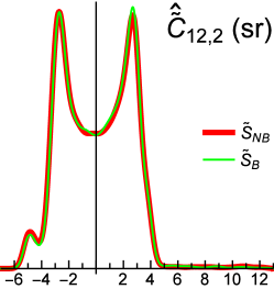
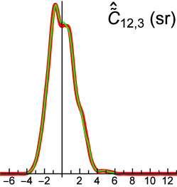
Refer to caption
(a) N=2𝑁2N=2
Refer to caption
(b) N=3𝑁3N=3
Refer to caption
(c) N=4𝑁4N=4
Figure 4: Distribution of the angular power spectrum estimator Eqn.Β (64) of the first N𝑁N events received. At just a few events, the distributions are wide, and there is no significant difference between the two different skymaps.

We begin analyzing the results by comparing the distribution of power spectrum estimates at fixed N𝑁N for each sky. Fig.Β 4 shows the distributions for the first few events. Interestingly, the estimator at 2 events shows a strong bimodal distribution, but this quickly collapses to a more typical bell curve by N=4𝑁4N=4. Initially, the distributions are very wide compared to the expectation value, and the distributions from the two skymaps cannot be distinguished at this number of trials.
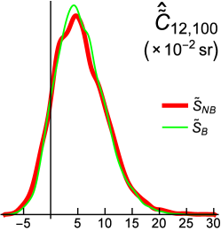
Refer to caption
(a) N=100𝑁100N=100
Β Β Β Β Β Οƒ^N​B=(4.77Β±0.60)Γ—10βˆ’2subscript^πœŽπ‘π΅plus-or-minus4.770.60superscript102\hat{\sigma}_{N\!B}=(4.77\pm 0.60)\times 10^{-2} sr
Β Β Β Β Β Οƒ^B=(4.47Β±0.55)Γ—10βˆ’2subscript^𝜎𝐡plus-or-minus4.470.55superscript102\hat{\sigma}_{B}=(4.47\pm 0.55)\times 10^{-2} sr
Β Β Β Β Β ΟƒN​B=4.74Γ—10βˆ’2subscriptπœŽπ‘π΅4.74superscript102\sigma_{N\!B}=4.74\times 10^{-2} sr
Β Β Β Β Β ΟƒB=4.52Γ—10βˆ’2subscript𝜎𝐡4.52superscript102\sigma_{B}=4.52\times 10^{-2} sr
Refer to caption
(b) N=1000𝑁1000N=1000
Β Β Β Β Β Οƒ^N​B=(1.03Β±0.12)Γ—10βˆ’2subscript^πœŽπ‘π΅plus-or-minus1.030.12superscript102\hat{\sigma}_{N\!B}=(1.03\pm 0.12)\times 10^{-2} sr
Β Β Β Β Β Οƒ^B=(0.96Β±0.11)Γ—10βˆ’2subscript^𝜎𝐡plus-or-minus0.960.11superscript102\hat{\sigma}_{B}=(0.96\pm 0.11)\times 10^{-2} sr
Β Β Β Β Β ΟƒN​B=1.05Γ—10βˆ’2subscriptπœŽπ‘π΅1.05superscript102\sigma_{N\!B}=1.05\times 10^{-2} sr
Β Β Β Β Β ΟƒB=0.95Γ—10βˆ’2subscript𝜎𝐡0.95superscript102\sigma_{B}=0.95\times 10^{-2} sr
Refer to caption
(c) N=10000𝑁10000N=10000
Β Β Β Β Β Οƒ^N​B=(0.312Β±0.037)Γ—10βˆ’2subscript^πœŽπ‘π΅plus-or-minus0.3120.037superscript102\hat{\sigma}_{N\!B}=(0.312\pm 0.037)\times 10^{-2} sr
Β Β Β Β Β Οƒ^B=(0.282Β±0.033)Γ—10βˆ’2subscript^𝜎𝐡plus-or-minus0.2820.033superscript102\hat{\sigma}_{B}=(0.282\pm 0.033)\times 10^{-2} sr
Β Β Β Β Β ΟƒN​B=0.314Γ—10βˆ’2subscriptπœŽπ‘π΅0.314superscript102\sigma_{N\!B}=0.314\times 10^{-2} sr
Β Β Β Β Β ΟƒB=0.279Γ—10βˆ’2subscript𝜎𝐡0.279superscript102\sigma_{B}=0.279\times 10^{-2} sr
Figure 5: Distribution of the angular power spectrum estimator Eqn.Β (64) after observation of 100, 1000, and 10 000 events. Note the changing scale of the axis. As N𝑁N increases, the distributions become narrower, centered on the correct power spectrum of C~12=0.0544subscript~𝐢120.0544\tilde{C}_{12}=0.0544 sr. The standard deviations Οƒ^^𝜎\hat{\sigma} of these distributions are specified in the subcaptions, estimated with Eqns.Β (121)–(124). The skymap S~Bsubscript~𝑆𝐡\tilde{S}_{B} with the negative open bispectrum is consistently producing a slightly narrower distribution, though the difference is not statistically significant for each case individually. However, the standard deviations consistently agree with the expected values Οƒ=(𝒱​ar​[C~^12,N])1/2𝜎superscript𝒱ardelimited-[]subscript^~𝐢12𝑁12\sigma=(\mathscr{V}\!\!\text{\it ar}\,[\hat{\tilde{C}}_{12,N}])^{1/2} from Eqn.Β (3.3) to a better precision than their uncertainties indicate.

It is demonstrated in Fig.Β 5 that, as N𝑁N increases, the probability distribution of the power spectrum narrows, converging to the actual power spectrum. Comparing the C~^β„“,Nsubscript^~𝐢ℓ𝑁\hat{\tilde{C}}_{\ell,N} distributions of the two skymaps, the distribution from S~Bsubscript~𝑆𝐡\tilde{S}_{B} is narrower at higher N𝑁N. The unbiased estimator of the variance 𝒱​ar​[C~^tr]𝒱ardelimited-[]superscript^~𝐢tr\mathscr{V}\!\!\text{\it ar}\,[\hat{\tilde{C}}^{\text{tr}}] of the power spectra C~1tr,C~2tr,…,C~Ntrtrsuperscriptsubscript~𝐢1trsuperscriptsubscript~𝐢2tr…superscriptsubscript~𝐢subscript𝑁trtr\tilde{C}_{1}^{\text{tr}},\tilde{C}_{2}^{\text{tr}},\dotsc,\tilde{C}_{N_{\text{tr}}}^{\text{tr}} observed after Ntrsubscript𝑁trN_{\text{tr}} trials is the usual result

𝒱​ar^​[C~^tr]=1Ntrβˆ’1β€‹βˆ‘p=1Ntr(C~ptrβˆ’C~^tr)2,^𝒱ardelimited-[]superscript^~𝐢tr1subscript𝑁tr1superscriptsubscript𝑝1subscript𝑁trsuperscriptsuperscriptsubscript~𝐢𝑝trsuperscript^~𝐢tr2\widehat{\mathscr{V}\!\!\text{\it ar}}\,[\hat{\tilde{C}}^{\text{tr}}]=\frac{1}{N_{\text{tr}}-1}\sum_{p=1}^{N_{\text{tr}}}\left(\tilde{C}_{p}^{\text{tr}}-\hat{\tilde{C}}^{\text{tr}}\right)^{2}, (121)

where the estimated power spectrum from trials is

C~^tr=1Ntrβ€‹βˆ‘p=1NtrC~ptr.superscript^~𝐢tr1subscript𝑁trsuperscriptsubscript𝑝1subscript𝑁trsuperscriptsubscript~𝐢𝑝tr\hat{\tilde{C}}^{\text{tr}}=\frac{1}{N_{\text{tr}}}\sum_{p=1}^{N_{\text{tr}}}\tilde{C}_{p}^{\text{tr}}. (122)

To determine whether a measured difference in the distribution width from the two skymaps is significant, we estimate the variance of our variance estimator to see how precisely 𝒱​ar​[C~^tr]𝒱ardelimited-[]superscript^~𝐢tr\mathscr{V}\!\!\text{\it ar}\,[\hat{\tilde{C}}^{\text{tr}}] was resolved at the present number of trials. It is a straightforward exercise to show that

𝒱​ar^​[𝒱​ar^​[C~^tr]]=^𝒱ardelimited-[]^𝒱ardelimited-[]superscript^~𝐢trabsent\displaystyle\widehat{\mathscr{V}\!\!\text{\it ar}}\,\left[\widehat{\mathscr{V}\!\!\text{\it ar}}\,[\hat{\tilde{C}}^{\text{tr}}]\right]= 1(Ntrβˆ’2)​(Ntrβˆ’3)[βˆ‘p=1Ntr(C~ptrβˆ’C~^tr)4\displaystyle\ \frac{1}{(N_{\text{tr}}-2)(N_{\text{tr}}-3)}\Bigg{[}\sum_{p=1}^{N_{\text{tr}}}\left(\tilde{C}_{p}^{\text{tr}}-\hat{\tilde{C}}^{\text{tr}}\right)^{4}
βˆ’(Ntrβˆ’3Ntr)(𝒱​ar^[C~^tr])2].\displaystyle-\left(N_{\text{tr}}-\frac{3}{N_{\text{tr}}}\right)\left(\widehat{\mathscr{V}\!\!\text{\it ar}}\,[\hat{\tilde{C}}^{\text{tr}}]\right)^{2}\Bigg{]}. (123)

Then the standard deviation and its uncertainty are estimated as

Οƒ^Ctr=(𝒱​ar^​[C~^tr])1/2Β±(𝒱​ar^​[𝒱​ar^​[C~^tr]])1/4.subscript^𝜎superscript𝐢trplus-or-minussuperscript^𝒱ardelimited-[]superscript^~𝐢tr12superscript^𝒱ardelimited-[]^𝒱ardelimited-[]superscript^~𝐢tr14\hat{\sigma}_{C^{\text{tr}}}=\left(\widehat{\mathscr{V}\!\!\text{\it ar}}\,[\hat{\tilde{C}}^{\text{tr}}]\right)^{1/2}\pm\left(\widehat{\mathscr{V}\!\!\text{\it ar}}\,\left[\widehat{\mathscr{V}\!\!\text{\it ar}}\,[\hat{\tilde{C}}^{\text{tr}}]\right]\right)^{1/4}. (124)

These estimates are presented in Fig.Β 5 for the distributions shown there. The standard deviation from the skymap S~N​Bsubscript~𝑆𝑁𝐡\tilde{S}_{N\!B} is denoted Οƒ^N​Bsubscript^πœŽπ‘π΅\hat{\sigma}_{N\!B}, and Οƒ^Bsubscript^𝜎𝐡\hat{\sigma}_{B} is the standard deviation of the estimates from S~Bsubscript~𝑆𝐡\tilde{S}_{B}. The measured standard deviations are in excellent agreement with the expected values determined with Eqn.Β (3.3). Additionally, for N=10000𝑁10000N=10000, ΟƒBsubscript𝜎𝐡\sigma_{B} is at 1ΟƒπœŽ\sigma tension with Οƒ^N​Bsubscript^πœŽπ‘π΅\hat{\sigma}_{N\!B}, and ΟƒN​BsubscriptπœŽπ‘π΅\sigma_{N\!B} is at 1ΟƒπœŽ\sigma tension with Οƒ^Bsubscript^𝜎𝐡\hat{\sigma}_{B}.

Refer to caption
(a) N=10𝑁10N=10
Refer to caption
(b) N=100𝑁100N=100
Refer to caption
(c) N=1000𝑁1000N=1000
Figure 6: Uncertainty estimates of the power spectrum for the S~N​Bsubscript~𝑆𝑁𝐡\tilde{S}_{N\!B} skymap. Thick curve: distribution of the angular power spectrum’s full uncertainty estimator s​|𝒱​ar^​[C~^12,N]|1/2𝑠superscript^𝒱ardelimited-[]subscript^~𝐢12𝑁12s\left|\widehat{\mathscr{V}\!\!\text{\it ar}}\,[\hat{\tilde{C}}_{12,N}]\right|^{1/2} with s𝑠s the sign of the variance estimate. Thick vertical line: expected full uncertainty determined from the known skymap. Thin curve: distribution of the Cβ„“subscript𝐢ℓC_{\ell}-only uncertainty estimator. Thin vertical line: actual value of the Cβ„“subscript𝐢ℓC_{\ell}-only uncertainty. Light rectangle: measured uncertainty from the simulated trials.
Refer to caption
(a) N=10𝑁10N=10
Refer to caption
(b) N=100𝑁100N=100
Refer to caption
(c) N=1000𝑁1000N=1000
Figure 7: Same as Fig.Β 6 for the S~Bsubscript~𝑆𝐡\tilde{S}_{B} skymap. At N=1000𝑁1000N=1000, the Cβ„“subscript𝐢ℓC_{\ell}-only variance is no longer consistent with the measured standard deviation of the distribution, making the secondary bispectrum and trispectrum effects statistically interesting.

Having determined estimators for all the spectra up to N=1000𝑁1000N=1000, we can test the effectiveness of the full variance estimator Eqn.Β (88) by considering its statistical distribution, compared to the Cβ„“subscript𝐢ℓC_{\ell}-only estimator from substituting C~^β„“,Nsubscript^~𝐢ℓ𝑁\hat{\tilde{C}}_{\ell,N} for C~β„“subscript~𝐢ℓ\tilde{C}_{\ell} in Eqn.Β (102). The uncertainty of the power spectrum is to be given by the square root of the variance. Though the variance estimator is unbiased, at low event counts the distribution of the estimator is so wide as to allow negative estimates of the variance. For visualization purposes, we will plot the root of negative variances as negative (rather than imaginary) uncertainties. The results for the full estimator are shown in the thick curves of Figs.Β 6 and 7. Shown in the thin curves are the Cβ„“subscript𝐢ℓC_{\ell}-only estimator. The actual values of these uncertainties in terms of the known sky distributions are shown by vertical lines. The shaded region is the 1ΟƒπœŽ\sigma measurement of the uncertainty Οƒ^Ctrsubscript^𝜎superscript𝐢tr\hat{\sigma}_{C^{\text{tr}}} from the variation in the measured power spectra of the simulated trials.

The N=10𝑁10N=10 plots reveal how unreliable the variance estimators are at low event counts. A significant fraction of trials produce negative variances, but the Cβ„“subscript𝐢ℓC_{\ell}-only variance is more reliable and more accurate, even though it is biased. At N=100𝑁100N=100, negative variances are very rare, and the width of the error’s distribution is within an order of magnitude, making it suitable for use in error estimation. Both variance estimators are consistent with the simulation. At N=1000𝑁1000N=1000, the width of the error estimators is around 10%. For the S~N​Bsubscript~𝑆𝑁𝐡\tilde{S}_{N\!B} skymap, both estimators agree with the simulation. Since there is no bispectrum, only the small trispectrum effect causes the small separation of the full error from the Cβ„“subscript𝐢ℓC_{\ell}-only error. In the S~Bsubscript~𝑆𝐡\tilde{S}_{B} skymap, the significant negative bispectrum causes the full error estimate to be reduced even further from the Cβ„“subscript𝐢ℓC_{\ell}-only estimate. The simulation exhibits a similar downward shift in its standard deviation Οƒ^Ctrsubscript^𝜎superscript𝐢tr\hat{\sigma}_{C^{\text{tr}}}, such that the Cβ„“subscript𝐢ℓC_{\ell}-only estimate is at 1ΟƒπœŽ\sigma tension with the simulation. This supports the validity of the work in this paper.

These experiments suggest that the unbiased variance estimator may only be reliable at estimating the actual variance when a power spectrum signal has been resolved. It is recommended that early analyses use the shot noise variance Eqn.Β (57) until C~β„“=0subscript~𝐢ℓ0\tilde{C}_{\ell}=0 is no longer consistent with that uncertainty estimate. At this point, the Cβ„“subscript𝐢ℓC_{\ell}-only uncertainty estimate will probably make the uncertainty large enough so that zero power is consistent. Once signal is again appearing, then at this stage the full unbiased uncertainty estimator should be reliable and most desirable.

Additional simulations will have the ability to produce more significant evidence supporting the new theoretical results, and determine more precise protocols for their safe usage.

5 Discussion: Implications for Experiments

We now discuss implications of the new results on experiments.

In order to understand the effect that these results will have on the Fermi-LAT γ𝛾\gamma-ray power spectrum measurement, one needs to determine estimates of the composite power spectrum C~^β„“,N(2)superscriptsubscript^~𝐢ℓ𝑁2\hat{\tilde{C}}_{\ell,N}^{(2)} and open bispectrum C~^β„“,N(3)superscriptsubscript^~𝐢ℓ𝑁3\hat{\tilde{C}}_{\ell,N}^{(3)} of the events in each energy bin. If these are negligible, then the results are well described with a Cβ„“subscript𝐢ℓC_{\ell}-only variance if making a skymap measurement, or with the cosmic variance with noise estimate if carrying out a cosmic mean analysis for sources on linear cosmological distance scales (that are Gaussian-distributed). Given their observed small variation in C~^β„“,N∼10βˆ’5similar-tosubscript^~𝐢ℓ𝑁superscript105\hat{\tilde{C}}_{\ell,N}\sim 10^{-5} sr, then one would expect C~^β„“,N(2)superscriptsubscript^~𝐢ℓ𝑁2\hat{\tilde{C}}_{\ell,N}^{(2)} to be of a similar magnitude, and therefore negligible compared to (2​ℓ+1)βˆ’1superscript2β„“11(2\ell+1)^{-1} of the shot noise term.

The Fermi-LAT’s measurement of C^β„“,Nsubscript^𝐢ℓ𝑁\hat{C}_{\ell,N} in the highest energy bin from 10.4 GeV to 50.0 GeV was shown to have been a bit underestimated when compared to the power spectrum of point sources subsequently detected after the anisotropy analysis was completed (Broderick et al., 2013a). It is intriguing this tension could be explained if that energy bin had a significant, positive open bispectrum. However, before estimates of the higher-order uncertainty contributions can be made using the formulas derived in this paper, they must be modified to additionally take into account the masking of parts of the sky and the non-uniform exposure map.

If a significant open bispectrum is detected in the diffuse γ𝛾\gamma-ray background, there will be an unfortunate decrease in significance of the measured power spectrum, but this would be in exchange for the exciting detection of higher-order angular correlations that would be very constraining for source population models. Such an observation would indicate significant departure from the galaxy distribution on the scales of structure which is Gaussian-distributed, suggesting a source of gamma-rays from a more local distribution. However, if it is found that C~β„“subscript~𝐢ℓ\tilde{C}_{\ell} has been correctly measured, this immediately puts new bounds on the magnitude of the open bispectrum C~β„“(3)superscriptsubscript~𝐢ℓ3\tilde{C}_{\ell}^{(3)}.

Extragalactic sources correlated with large scale structure on linear cosmological distance scales would be expected to be Gaussian-distributed to within Poisson noise if sparse (such as active galactic nuclei), or Gaussian cosmic variance if dense (for instance, star-forming galaxies). The presence of a large bispectrum would be an indication of a population of sources that is either extragalactic at sub-Mpc scales (from galaxies in the local Universe), or Galactic. Example Galactic sources may be a population of unresolved pulsars (Calore, Di Mauro, & Donato, 2014), or annihilation in dark matter subhalos (Campbell & Beacom, 2013).

A way to probe the presence of an angular bispectrum affecting the power spectrum measurement is to analyze the time-sequence C~^β„“,Nsubscript^~𝐢ℓ𝑁\hat{\tilde{C}}_{\ell,N} as a function of N𝑁N. This value of the estimated power spectrum wanders randomly around the actual skymap’s power spectrum, with an amplitude that is indicative of the magnitude of the statistical uncertainty. With the collection of additional data, this amplitude diminishes in magnitude roughly as Nβˆ’1superscript𝑁1N^{-1} and the estimator converges to the skymap’s power spectrum. However, an early transition to a signal-dominated error that shrinks as Nβˆ’1/2superscript𝑁12N^{-1/2}, before the power spectrum has been resolved, would be evidence for the presence of a significant open bispectrum. The robustness of detecting the bispectrum using a single time-sequence of data can be tested with simulations in future work.

Now consider other experiments interested in measuring angular power spectra. For the angular distribution probes of cosmology, such as galaxy surveys, the amount of data is usually so high that the statistical uncertainty is dominated by cosmic variance and the new findings in this paper have no new effect. However, if galaxy distances can be made precise enough to allow accurate separation into such thin redshift slices that the number of galaxies per redshift slice is ≲106less-than-or-similar-toabsentsuperscript106\la 10^{6}, then cosmic variance of each redshift slice may no longer be the dominant statistical uncertainty and the new methods in this paper would be of use.

When counting objects such as galaxies, or blazars, etc., the role of the point spread function in Sec.Β 3 is replaced by a selection function that specifies the completeness of observations. The β€˜skymap’ refers in this case to the complete map of the objects of interest.

For high-energy radiation events, the skymap is the complete apparent flux map of all radiation sources convolved by propagation effects. The propagation effects are most severe for charged cosmic rays which are deflected and hard-scattered within the medium. Since γ𝛾\gamma-rays and neutrinos interact less, the measurement of their high-energy angular power spectrum in different energy bins has the potential to identify the sources. One can use this information to separate distinct components of radiation from different sources (Hensley, Siegal-Gaskins, & Pavlidou, 2013). Even hard spectral features too faint to be seen in the flux spectrum could still be observed in anisotropies (Zhang & Beacom, 2004; Campbell & Beacom, 2013). If the γ𝛾\gamma-rays or neutrinos have a particular angular power spectrum that matches the distribution of a potential source, this would be strong evidence for the origin of the high-energy radiation, motivating a cross-correlation analysis to be carried out between the radiation and that particular point source catalog (e.g., Xia et al., 2011; Ando, Benoit-LΓ©vy, & Komatsu, 2014).

A natural application of these methods is to IceCube neutrino data. The astrophysical component in the energy range 30 TeV–2 PeV has a flux that produces roughly 10 events per year. If the source is stationary with a large fluctuation power spectrum ∼10βˆ’2similar-toabsentsuperscript102\sim 10^{-2} sr and small or negative open bispectrum, then the power spectrum could be begin to be resolved within 10 years of data. Another interesting analysis is determination of the power spectrum of the lower energy neutrinos from IceCube; the presence of an anisotropic astrophysical component can be searched for among the highly numerous and isotropic atmospheric neutrinos.

Significant power spectra in the arrival direction of charged cosmic rays would indicate angular clustering that potentially contains information about the distribution of nearby sources and the structure of fields and material in the rays’ path to us (Sutherland, Baughman, & Beatty, 2012; Keivani, Farrar, & Sutherland, 2015). A new way to test for the presence of a significant dipole distribution is to determine if the β„“=1β„“1\ell=1 component of the power spectrum is significant. If this amplitude is significant, the phase of the dipole can be ascertained from the values of the three β„“=1β„“1\ell=1 spherical harmonic transforms.

6 Conclusions

To summarize, we have carried out an error analysis of the angular power spectrum of a finite set of points on a sphere. The statistical framework is modeled with only two postulates: a stationary β€˜skymap’ distribution of sources S​(𝐧)𝑆𝐧S(\mathbf{n}) and the assumption of independence of the detected events. For this analysis, the observation of the points is made with uniform efficiency and exposure over the entire sphere.

We have presented an estimator of the skymap’s power spectrum in Eqn.Β (10) or Eqn.Β (64) that is unbiased with respect to a fixed number of observed events N𝑁N, and we determined the variance of the measured power spectrum as a function only of N𝑁N and S​(𝐧)𝑆𝐧S(\mathbf{n}) in Eqn.Β (13) or Eqn.Β (3.3). The power spectrum estimator is consistent with usual pseudo-spectrum techniques, and its statistical variance is found to agree at leading order with previous analytic estimates.

New, previously unquantified effects of the power spectrum variance have been discovered that are generated by three effects: the power spectrum at neighboring multipoles (the composite power spectrum Cβ„“(2)superscriptsubscript𝐢ℓ2C_{\ell}^{(2)}), the bispectrum of the skymap (in a form called the open bispectrum Cβ„“(3)superscriptsubscript𝐢ℓ3C_{\ell}^{(3)}), and the skymap’s trispectrum (given by the disjoint trispectrum Cβ„“(4)superscriptsubscript𝐢ℓ4C_{\ell}^{(4)}). A study of these new higher-order spectra is presented in AppendixΒ A. They are the only possible β€˜two-correlator’ spectra, and are also the only spherical tensors that can be derived from rank 2 spherical transforms of the skymap.

These new higher order effects will be negligible under certain conditions that have been precisely identified. In this work, the power spectrum variance is called Cβ„“subscript𝐢ℓC_{\ell}-only at those values of N𝑁N where these new higher-order effects are negligible, corresponding to error estimates used in previous works. The new terms, with the open bispectrum in particular, have the potential to add orders of magnitude to the variance. Thus, the neglect of these new terms may result in spurious detections of the power spectrum. A negative open bispectrum causes the signal term of the variance to be smaller than Cβ„“subscript𝐢ℓC_{\ell}-only.

The behavior of the power spectrum variance is classified by two regimes in N𝑁N: in the small-N𝑁N regime, the variance is dominated by a shot term that goes as Nβˆ’2superscript𝑁2N^{-2} (for N≫1much-greater-than𝑁1N\gg 1); when N𝑁N is large, a signal term dominates and the variance goes as Nβˆ’1superscript𝑁1N^{-1}. The composite power spectrum minus disjoint trispectrum is a new contribution to the shot term, added to the shot noise variance. The signal term, which in previous work was the variance due to the power spectrum itself, is found to have additional terms from the open bispectrum minus disjoint trispectrum.

An unbiased estimator of the power spectrum’s variance is identified in Eqn.Β (88) or Eqn.Β (90), calculated from the data. Remarkably, this estimate is made without any prior assumptions about properties of the skymap spatial distribution. Efficient, highly parallelizable codes have been shown to be very efficient at calculating this variance from position data. This makes these exact methods viable for use (at least for the full sky, uniform exposure limit) to quite large counts, relaxing the necessity of binning the data into pixels on the sphere, which either introduces the need to correct for β€˜pixel’ features in the power spectrum, or uses a large number of tiny pixels that requires more computation to determine the spectrum than the exact method.

These estimators are very important, providing a means for experiments to test for the presence of higher-order contributions to the power spectrum uncertainty. The presence of a large open bispectrum in the diffuse γ𝛾\gamma-ray background measured by Fermi-LAT would decrease the significance of the measured power spectrum, but would provide exciting new information about the distribution of the source populations. On the other hand, verification of the existing power spectrum measurements would provide stringent bounds on the magnitude of non-Gaussianities in the distribution. Those γ𝛾\gamma-ray distributions consistent with being Gaussian to within cosmic variance are consistent with being produced by extragalactic sources over linear cosmological distances. The presence of non-Gaussianities would suggest the presence of a population of more local sources, either near-extragalactic, or Galactic sources.

We showed how these results can be applied to a statistical model of the spatial distribution of the skymap by considering an example analysis of a Gaussian-distributed skymap. In this context, the prediction of the power spectrum is subject to cosmic variance from statistical variations between different skymap realizations of the Gaussian process. The open bispectrum vanishes for Gaussian distributions. Otherwise, the previous analytic estimates for the uncertainty of the power spectrum in these measurements was reproduced to first order, with additional higher order contributions from the composite power spectrum and disjoint trispectrum as expressed in Eqn.Β (96). These new contributions become important at large β„“β„“\ell since these new terms are not suppressed by (2​ℓ+1)βˆ’1superscript2β„“11(2\ell+1)^{-1}, as is the case for the standard terms. The usual uncertainty is restored when enough data is collected for the statistical uncertainty to be dominated by the cosmic variance. Thus, power spectrum measurements of large data sets that are cosmic variance limited remain unaffected by the new findings.

The effect of the instrument point spread function (PSF) on the power spectrum measurement is found to simply be that the measured spectra are of the skymap convolved with the PSF. However, further effects may be induced by asymmetric PSFs on the inference of the cosmic mean power spectrum of a modeled ensemble of Universes.

Simulations were carried out of two skymaps of equivalent power spectrum, but one without open bispectrum and the other with significant open bispectrum. The standard deviation of power spectrum estimates using the simulated data were shown to prefer the variance results of this paper with the bispectrum effect over the Cβ„“subscript𝐢ℓC_{\ell}-only variance.

The new formalism in this paper is important for smaller datasets, such as for events of incident high-energy radiation, where the power spectrum provides information about the distribution of sources and propagation effects. After around 106superscript10610^{6} detected events, it is likely more efficient to use pixeled-sky estimates for which the uncertainty results presented here can be adapted.

Acknowledgments

For informative discussions, suggestions, or comments on an early version of this manuscript, I thank Shin’ichiro Ando, AurΓ©lien Benoit-LΓ©vy, Jonathan Blazek, Alessandro Cuoco, Mattia Fornasa, Nicolao Fornengo, Chris Gordon, Eric Huff, Kevin Huffenberger, Boris Leistedt, Peter Melchior, Ashley Ross, BjΓΆrn Malte SchΓ€fer, Hee-Jong Seo, Paul Sutter, David Weinberg, and especially thank John Beacom, Chris Hirata, and Eiichiro Komatsu for their additional time and particularly insightful feedback. The program to generate the sphere distribution plots was inspired by β€˜Nodal Domains of Spherical Harmonics’ from the Wolfram Demonstrations Project, contributed by Michael Trott. This research is partly funded by NSF Grant PHY-1101216 awarded to John Beacom.

References

  • Ando & Komatsu (2006) Ando S., Komatsu E., 2006, Phys. Rev. D, 73, 023521
  • Ando & Komatsu (2013) Ando S., Komatsu E., 2013, Phys. Rev. D, 87, 123539
  • Ando et al. (2007) Ando S., Komatsu E., Narumoto T., Totani T., 2007, Phys. Rev. D, 75, 063519
  • Ando, Benoit-LΓ©vy, & Komatsu (2014) Ando S., Benoit-LΓ©vy A., Komatsu E., 2014, Phys. Rev. D, 90, 023514
  • Bogaert, Michiels, & Fostier (2012) Bogaert I., Michiels B., Fostier J., 2012, Siam. J. Sci. Comput., 34, C83
  • Broderick et al. (2013a) Broderick A., Pfrommer C., Puchwein E., Chang P., 2013, arXiv:1308.0015
  • Broderick et al. (2013b) Broderick A., Pfrommer C., Puchwein E., Chang P., arXiv:1308.0340
  • Calore et al. (2014) Calore F., De Romeri V., Di Mauro M., Donato F., Herpich J., MacciΓ² A. V., Maccione L., 2014, MNRAS, 442, 1151
  • Calore, Di Mauro, & Donato (2014) Calore F., Di Mauro M., Donato F., 2014,Β Β Β Β Β  arXiv:1406.2706
  • Campbell & Beacom (2013) Campbell S. S., Beacom J. F., 2013, arXiv:1312.3945
  • Campbell & Dutta (2011) Campbell S., Dutta B., 2011, Phys. Rev. D, 84, 075004
  • Campbell, Dutta, & Komatsu (2010) Campbell S., Dutta B., Komatsu E., 2010, Phys. Rev. D, 82, 095007
  • Cuoco, Komatsu, & Siegal-Gaskins (2012) Cuoco A., Komatsu E., Siegal-Gaskins J. M., 2012, Phys. Rev. D, 86, 063004
  • Desiati (2014) Desiati P., for the IceCube Collaboration, 2014, Nucl. Instrum. Meth. A, 742, 199
  • Di Mauro et al. (2014) Di Mauro M., Cuoco A., Donato F., Siegal-Gaskins J. M., 2014, arXiv:1407.3275
  • Durrer (2008) Durrer R., 2008, The Cosmic Microwave Background. Cambridge University Press, Cambridge
  • Edmonds (1957) Edmonds A. R., 1957, Angular Momentum in Quantum Mechanics, 2nd Ed., 4th Printing 1996. Princeton University Press, Princeton
  • Efstathiou (2004) Efstathiou G., 2004, MNRAS, 349, 603
  • Fermi-LAT Collaboration (2012) Fermi-LAT Collaboration, 2012, Phys. Rev. D, 85, 083007
  • Fisher, Schar, & Lahav (1994) Fisher K. B., Scharf C. A., Lahav O., 1994, MNRAS, 266, 219
  • Fisher (1953) Fisher R., 1953, Proc. R. Soc. Lond. A, 217, 295
  • Giaccari (2013) Giaccari U. G., for the Pierre Auger Collaboration, 2013, PoS (EPS-HEP 2013), 397
  • GΓ³mez-Vargas et al. (2013) GΓ³mez-Vargas G. A. et al., 2012, in Omodei N, Brandt T., Wilson-Hodge C., eds., Proc. Intl. Fermi Symp. 4, Stanford, p. 191
  • Hanbury Brown & Twiss (1957) Hanbury Brown R., Twiss R. Q., 1957, Proc. R. Soc. Lond. A, 242, 300
  • Harding & Abazajian (2012) Harding P. J., Abazajian K. N., 2012, JCAP, 1211, 026
  • Harnois-DΓ©raps & Pen (2013) Harnois-DΓ©raps J., Pen U.-L., 2013, MNRAS, 431, 3349
  • Harrison (1970) Harrison E. R., 1970, Phys. Rev. D, 1, 2726
  • Harrison (2009) Harrison J., 2009, in Proceedings of the 19th IEEE Symposium on Computer Arithmetic, IEEE Computer Society, Portland, p. 104
  • HAWC Collaboration (2014) HAWC Collaboration, 2014, arXiv:1408.4805
  • Hayes, Brunner, & Ross (2012) Hayes B., Brunner R., Ross A., 2012, MNRAS, 421, 2043
  • Hensley, Siegal-Gaskins, & Pavlidou (2013) Hensley B. S., Siegal-Gaskins J. M., Pavlidou V., 2013, MNRAS, 433, 591
  • Hinshaw et al. (2007) Hinshaw G. et al., 2007, ApJS, 170, 288
  • Hivon et al. (2002) Hivon E., GΓ³rski K. M., Netterfield, C. B., Crill B. P., Prunet S., Hansen F., 2002, ApJ, 567, 2
  • Ho et al. (2012) Ho S. et al., 2012, ApJ, 761, 14
  • Ho et al. (2013) Ho S. et al., 2013, arXiv:1311.2597
  • Holmes et al. (2008) Holmes W. A., Bock J. J., Crill B. P., Koch T. C., Jones W. C., Lange A. E., Paine C. G., 2008, Appl. Opt., 47, 5996
  • Hu (2001) Hu W., 2001, Phys. Rev. D, 64, 083005
  • IceCube Collaboration (2013) IceCube Collaboration, 2013, Phys. Rev. Lett., 111, 021103
  • IceCube Collaboration (2014a) IceCube Collaboration, 2014, arXiv:1405.5303
  • IceCube Collaboration (2014b) IceCube Collaboration, 2014, arXiv:1406.6868
  • IceCube Collaboration (2014c) IceCube Collaboration, 2014, arXiv:1408.0634
  • Ivanov et al. (2014) Ivanov A. A.,Β Β  Krasilnikov A. D.,Β Β  Pravdin M. I.,Β  Sabourov A. V., 2014, arXiv:1407.1583
  • Jeltes et al. (2007) Jeltes T. et al., 2007, Nature, 445, 402
  • Keivani, Farrar, & Sutherland (2015) Keivani A., Farrar G. R., Sutherland M., 2015, Astropart. Phys., 61, 47
  • Knox (1995) Knox L., 1995, Phys. Rev. D, 52, 4307
  • Knuth (1997) Knuth D., 1997, Art of Computer Programming, Vol. 2: Seminumerical Algorithms, 3rd Ed. Addison-Wesley, Boston
  • Leistedt et al. (2013) Leistedt B., Peiris H. V., Mortlock D. J., Benoit-LΓ©vy A., Pontzen A., 2013, MNRAS, 435, 1857
  • Linsley (1975) Linsley J., 1975, Phys. Rev. Lett., 34, 1530
  • Molinari et al. (2014) Molinari D., Gruppuso A., Polenta G., Burigana C., De Rosa A., Natoli P., Finelli F., Paci F., 2014, MNRAS, 440, 957
  • Paykari, Starck, & Fadili (2012) Paykari P., Starck J.-L., Fadili M. J., 2012, A&A, 541, A74
  • Percival et al. (2004) Percival W. J. et al., 2004, MNRAS, 353, 1201
  • Planck Collaboration (2014) Planck Collaboration XV, 2014, A&A, in press
  • Ramond (2001) Ramond P., 2001, Front. Phys., 74, 1
  • Sachs & Wolfe (1967) Sachs R. K., Wolfe A. M., 1967, ApJ, 147, 73
  • Santander (2013) Santander M., for the IceCube Collaboration, 2013, Nucl. Instrum. Meth. A, 725, 85
  • SDSS Collaboration (2006) SDSS Collaboration, 2006, Phys. Rev. D, 74, 123507
  • Siegal-Gaskins & Pavlidou (2009) Siegal-Gaskins J. M., Pavlidou V., 2009, Phys. Rev. Lett., 102, 241301
  • Sutherland, Baughman, & Beatty (2012) Sutherland M. S., Baughman B. M., Beatty J. J., 2012, Astropart. Phys., 37, 17
  • Tamburro (2014) Tamburro A., for the IceCube Collaboration, 2014, Nucl. Instrum. Meth. A, 742, 35
  • Tegmark (1997) Tegmark M., 1997, Phys. Rev. D, 55, 5895
  • Tegmark (1997) Tegmark M., 1997, ApJ, 480, L87
  • Tegmark et al. (1997) Tegmark M., Taylor A. N., Heavens A. F, 1997, ApJ, 480, 22
  • Telescope Array Collaboration (2014) Telescope Array Collaboration, 2014, ApJ, 790, L21
  • Vallisneri (2008) Vallisneri M., 2008, Phys. Rev. D, 77, 042001
  • Westerhoff (2013) Westerhoff S., for the HAWC Collaboration, 2013, PoS (EPS-HEP 2013), 412
  • WMAP Collaboration (2013) WMAP Collaboration, ApJS, 2013, 208, 20
  • Xia et al. (2011) Xia J-Q., Cuoco A., Branchini E., Fornasa M., Viel M., 2011, MNRAS, 416, 2247
  • Zel’dovich (1972) Zel’dovich Y. B., 1972, MNRAS, 160, 1
  • Zhang & Beacom (2004) Zhang P.-J., Beacom J. F., 2004, ApJ, 614, 37
  • Zmuidzinas (2003) Zmuidzinas J., 2003, Appl. Opt., 42, 4989

Appendix A Rotationally Invariant Spherical Tensors

This appendix introduces the notations and formal mathematical structures that appear in the results of this paper. For further background on spherical tensors, their products, and their rotations, we recommend Edmonds (1957) and Hu (2001).

Spherical Tensors: Let 𝐧𝐧\mathbf{n} denote any unit position vector in 3 dimensional Euclidean space. In the context of this paper, spherical tensors are those generated by the spherical harmonic functions and any square-integrable scalar function S​(𝐧)𝑆𝐧S(\mathbf{n}) defined on the unit sphere. This is described below. Thus, these tensors inherit their coordinate transformation properties and symmetries from the spherical harmonics Yβ„“m​(𝐧)superscriptsubscriptπ‘Œβ„“π‘šπ§Y_{\ell}^{\,m}(\mathbf{n}).

Common conventions for the spherical harmonics are taken. They are normalized according to the orthonormality relation

∫d𝐧​[Yβ„“1m1​(𝐧)]βˆ—β€‹Yβ„“2m2​(𝐧)=Ξ΄β„“1​ℓ2​δm1​m2,differential-d𝐧superscriptdelimited-[]superscriptsubscriptπ‘Œsubscriptβ„“1subscriptπ‘š1𝐧superscriptsubscriptπ‘Œsubscriptβ„“2subscriptπ‘š2𝐧subscript𝛿subscriptβ„“1subscriptβ„“2subscript𝛿subscriptπ‘š1subscriptπ‘š2\int\mathrm{d}\mathbf{n}[Y_{\ell_{1}}^{\ m_{1}}(\mathbf{n})]^{*}Y_{\ell_{2}}^{\ m_{2}}(\mathbf{n})=\delta_{\ell_{1}\ell_{2}}\,\delta_{m_{1}m_{2}}, (125)

where * denotes complex conjugation, and Ξ΄x1​x2subscript𝛿subscriptπ‘₯1subscriptπ‘₯2\delta_{x_{1}x_{2}} is the Kronecker delta. It is important in this application to note that with this standard normalization, the spherical harmonics have physical units of inverse angle, which is equivalent to inverse length on the sphere.

The index β„“β„“\ell is often called the multipole. It specifies the angular diameter ΟˆβˆΌΟ€/β„“similar-toπœ“πœ‹β„“\psi\sim\pi/\ell of positive or negative regions of the spherical harmonics. Since the sphere is topologically compact, continuity of the spherical harmonics requires the spectrum of multipoles be discrete, and they are defined to take values β„“=0,1,2,….β„“012…\ell=0,1,2,\ldots.

The index mπ‘šm is sometimes called the azimuthal index. An azimuthal index of a spherical tensor must always be associated with one multipole index. However, note that a multipole index can generally have any number of azimuthal indices associated with it. For a given value of its associated multipole β„“β„“\ell, the azimuthal index spans the integer values βˆ’β„“β‰€mβ‰€β„“β„“π‘šβ„“-\ell\leq m\leq\ell, delineating the 2​ℓ+12β„“12\ell+1 orthogonal harmonic modes with angular scale Ο€/β„“πœ‹β„“\pi/\ell.

To generate spherical tensors that are invariant under rotations, it is convenient to introduce tensors with covariant azimuthal indices Sℓ​msubscriptπ‘†β„“π‘šS_{\ell m} and contravariant azimuthal indices Sβ„“msuperscriptsubscriptπ‘†β„“π‘šS_{\ell}^{\ m}, related by

Sℓ​mβ‰‘βˆ‘mβ€²=βˆ’β„“β„“gm,mβ€²(β„“)​Sβ„“mβ€²=(βˆ’1)m​Sβ„“βˆ’m,subscriptπ‘†β„“π‘šsuperscriptsubscriptsuperscriptπ‘šβ€²β„“β„“subscriptsuperscriptπ‘”β„“π‘šsuperscriptπ‘šβ€²superscriptsubscript𝑆ℓsuperscriptπ‘šβ€²superscript1π‘šsuperscriptsubscriptπ‘†β„“π‘šS_{\ell m}\equiv\sum_{m^{\prime}=-\ell}^{\ell}g^{(\ell)}_{m,m^{\prime}}S_{\ell}^{\ m^{\prime}}=(-1)^{m}S_{\ell}^{\ -m}, (126)

where the β„“β„“\ell-dimensional spherical metric tensor has components

gm,mβ€²(β„“)≑(βˆ’1)m​δm,βˆ’mβ€²,|m|≀ℓ.formulae-sequencesubscriptsuperscriptπ‘”β„“π‘šsuperscriptπ‘šβ€²superscript1π‘šsubscriptπ›Ώπ‘šsuperscriptπ‘šβ€²π‘šβ„“g^{(\ell)}_{m,m^{\prime}}\equiv(-1)^{m}\delta_{m,-m^{\prime}},\quad|m|\leq\ell. (127)

The rank of a spherical tensor is the number of multipole indices it contains, and the number of azimuthal indices for each multipole index. The full rank can be specified by a list of azimuthal ranks. For example, a rank (2,1,0) spherical tensor Sβ„“1,m11,m12,β„“2,m2,β„“3subscript𝑆subscriptβ„“1subscriptπ‘š11subscriptπ‘š12subscriptβ„“2subscriptπ‘š2subscriptβ„“3S_{\ell_{1},m_{11},m_{12},\ell_{2},m_{2},\ell_{3}} has 3 multipole indices of rank 2, 1, and 0, respectively. The rotation-invariant spherical tensors have only rank 0 multipole indices.

New spherical tensors can also be constructed by contracting a covariant and contravariant azimuthal index with the same multipole. For example, a rank 0 tensor Tβ„“subscript𝑇ℓT_{\ell} can be constructed from a rank 2 spherical tensor Sℓ​m1m2superscriptsubscript𝑆ℓsubscriptπ‘š1subscriptπ‘š2S_{\ell m_{1}}^{\ \ \ \ m_{2}} by contraction of the azimuthal indices,

Tβ„“=12​ℓ+1β€‹βˆ‘m=βˆ’β„“β„“Sℓ​mm.subscript𝑇ℓ12β„“1superscriptsubscriptπ‘šβ„“β„“superscriptsubscriptπ‘†β„“π‘šπ‘šT_{\ell}=\frac{1}{2\ell+1}\sum_{m=-\ell}^{\ell}S_{\ell m}^{\ \ \ m}. (128)

Spherical Transforms: Let S​(𝐧)𝑆𝐧S(\mathbf{n}) be a non-negative, real-valued, integrable function on the sphere. Then we may normalize S𝑆S without loss of generality such that

∫d​𝐧4​π​S~​(𝐧)=1,d𝐧4πœ‹~𝑆𝐧1\int\frac{\mathrm{d}\mathbf{n}}{4\pi}\tilde{S}(\mathbf{n})=1, (129)

where

S~​(𝐧)≑S​(𝐧)∫d​𝐧′4​π​S​(𝐧′).~𝑆𝐧𝑆𝐧dsuperscript𝐧′4πœ‹π‘†superscript𝐧′\tilde{S}(\mathbf{n})\equiv\frac{S(\mathbf{n})}{\int\frac{\mathrm{d}\mathbf{n}^{\prime}}{4\pi}S(\mathbf{n}^{\prime})}. (130)

Spherical tensors of any combination of non-zero rank multipoles can be generated from S~​(𝐧)βˆ’1~𝑆𝐧1\tilde{S}(\mathbf{n})-1 by spherical harmonic transforms, with the Yβ„“msuperscriptsubscriptπ‘Œβ„“π‘šY_{\ell}^{\,m} generating contravariant indices, and the complex conjugates (βˆ’1)m​Yβ„“βˆ’m=(Yβ„“m)βˆ—β‰‘Yℓ​mβˆ—superscript1π‘šsuperscriptsubscriptπ‘Œβ„“π‘šsuperscriptsuperscriptsubscriptπ‘Œβ„“π‘šsubscriptsuperscriptπ‘Œβ„“π‘š(-1)^{m}Y_{\ell}^{\,-m}=(Y_{\ell}^{\,m})^{*}\equiv Y^{*}_{\ell m} generating covariant indices.

The central spherical harmonic transform of S~​(𝐧)~𝑆𝐧\tilde{S}(\mathbf{n}) is a rank 1 spherical tensor.

S~ℓ​msubscript~π‘†β„“π‘š\displaystyle\tilde{S}_{\ell m} =∫d𝐧​Yℓ​mβˆ—β€‹(𝐧)​[S~​(𝐧)βˆ’1]absentdifferential-d𝐧subscriptsuperscriptπ‘Œβ„“π‘šπ§delimited-[]~𝑆𝐧1\displaystyle=\int\mathrm{d}\mathbf{n}\ Y^{*}_{\ell m}(\mathbf{n})\left[\tilde{S}(\mathbf{n})-1\right] (131)
S~β„“msuperscriptsubscript~π‘†β„“π‘š\displaystyle\tilde{S}_{\ell}^{\ m} =∫d𝐧​Yβ„“m​(𝐧)​[S~​(𝐧)βˆ’1]absentdifferential-d𝐧superscriptsubscriptπ‘Œβ„“π‘šπ§delimited-[]~𝑆𝐧1\displaystyle=\int\mathrm{d}\mathbf{n}\ Y_{\ell}^{\,m}(\mathbf{n})\left[\tilde{S}(\mathbf{n})-1\right] (132)

These tensors have units of angle. Since ∫d𝐧​Yβ„“m​(𝐧)=Ξ΄β„“,0​4​πdifferential-d𝐧superscriptsubscriptπ‘Œβ„“π‘šπ§subscript𝛿ℓ04πœ‹\int\mathrm{d}\mathbf{n}\,Y_{\ell}^{\,m}(\mathbf{n})=\delta_{\ell,0}\sqrt{4\pi}, then taking the central transform only adjusts the β„“=0β„“0\ell=0 component as

S~ℓ​m=∫d𝐧​Yℓ​mβˆ—β€‹(𝐧)​S~​(𝐧)βˆ’Ξ΄β„“,0​4​π.subscript~π‘†β„“π‘šdifferential-d𝐧subscriptsuperscriptπ‘Œβ„“π‘šπ§~𝑆𝐧subscript𝛿ℓ04πœ‹\tilde{S}_{\ell m}=\int\mathrm{d}\mathbf{n}\ Y^{*}_{\ell m}(\mathbf{n})\tilde{S}(\mathbf{n})-\delta_{\ell,0}\sqrt{4\pi}. (133)

Similarly, there are four different rank 2 spherical transforms of S𝑆S, which in this case are unitless.

S~ℓ​m1​m2subscript~𝑆ℓsubscriptπ‘š1subscriptπ‘š2\displaystyle\tilde{S}_{\ell m_{1}m_{2}} =∫d𝐧​Yℓ​m1βˆ—β€‹(𝐧)​Yℓ​m2βˆ—β€‹(𝐧)​[S~​(𝐧)βˆ’1]absentdifferential-d𝐧subscriptsuperscriptπ‘Œβ„“subscriptπ‘š1𝐧subscriptsuperscriptπ‘Œβ„“subscriptπ‘š2𝐧delimited-[]~𝑆𝐧1\displaystyle=\int\mathrm{d}\mathbf{n}\ Y^{*}_{\ell m_{1}}(\mathbf{n})Y^{*}_{\ell m_{2}}(\mathbf{n})\left[\tilde{S}(\mathbf{n})-1\right] (134)
S~ℓ​m1m2superscriptsubscript~𝑆ℓsubscriptπ‘š1subscriptπ‘š2\displaystyle\tilde{S}_{\ell m_{1}}^{\ \ \ \ m_{2}} =∫d𝐧​Yℓ​m1βˆ—β€‹(𝐧)​Yβ„“m2​(𝐧)​[S~​(𝐧)βˆ’1]absentdifferential-d𝐧subscriptsuperscriptπ‘Œβ„“subscriptπ‘š1𝐧superscriptsubscriptπ‘Œβ„“subscriptπ‘š2𝐧delimited-[]~𝑆𝐧1\displaystyle=\int\mathrm{d}\mathbf{n}\ Y^{*}_{\ell m_{1}}(\mathbf{n})Y_{\ell}^{\,m_{2}}(\mathbf{n})\left[\tilde{S}(\mathbf{n})-1\right] (135)
S~β„“m2m1superscriptsubscript~𝑆ℓsubscriptπ‘š2subscriptπ‘š1\displaystyle\tilde{S}_{\ell\ \ \ \,m_{2}}^{\ m_{1}} =∫d𝐧​Yβ„“m1​(𝐧)​Yℓ​m2βˆ—β€‹(𝐧)​[S~​(𝐧)βˆ’1]absentdifferential-d𝐧superscriptsubscriptπ‘Œβ„“subscriptπ‘š1𝐧subscriptsuperscriptπ‘Œβ„“subscriptπ‘š2𝐧delimited-[]~𝑆𝐧1\displaystyle=\int\mathrm{d}\mathbf{n}\ Y_{\ell}^{\,m_{1}}(\mathbf{n})Y^{*}_{\ell m_{2}}(\mathbf{n})\left[\tilde{S}(\mathbf{n})-1\right] (136)
S~β„“m1​m2superscriptsubscript~𝑆ℓsubscriptπ‘š1subscriptπ‘š2\displaystyle\tilde{S}_{\ell}^{\ m_{1}m_{2}} =∫d𝐧​Yβ„“m1​(𝐧)​Yβ„“m2​(𝐧)​[S~​(𝐧)βˆ’1]absentdifferential-d𝐧superscriptsubscriptπ‘Œβ„“subscriptπ‘š1𝐧superscriptsubscriptπ‘Œβ„“subscriptπ‘š2𝐧delimited-[]~𝑆𝐧1\displaystyle=\int\mathrm{d}\mathbf{n}\ Y_{\ell}^{\,m_{1}}(\mathbf{n})Y_{\ell}^{\,m_{2}}(\mathbf{n})\left[\tilde{S}(\mathbf{n})-1\right] (137)

Taking the central moment adjusted all of the multipoles on the diagonal of the azimuth indices,

S~ℓ​m1m2=∫d𝐧​Yℓ​m1βˆ—β€‹(𝐧)​Yβ„“m2​(𝐧)​S~​(𝐧)βˆ’Ξ΄m1m2.superscriptsubscript~𝑆ℓsubscriptπ‘š1subscriptπ‘š2differential-d𝐧subscriptsuperscriptπ‘Œβ„“subscriptπ‘š1𝐧superscriptsubscriptπ‘Œβ„“subscriptπ‘š2𝐧~𝑆𝐧superscriptsubscript𝛿subscriptπ‘š1subscriptπ‘š2\tilde{S}_{\ell m_{1}}^{\ \ \ \ m_{2}}=\int\mathrm{d}\mathbf{n}\ Y^{*}_{\ell m_{1}}(\mathbf{n})Y_{\ell}^{\,m_{2}}(\mathbf{n})\tilde{S}(\mathbf{n})-\delta_{m_{1}}^{\ \ \ m_{2}}. (138)

It is worth noting that the rankΒ 2 transforms can be expressed as sums of the rankΒ 1 transforms by applying the result for a product of spherical harmonics,

Yβ„“1m1​(𝐧)​Yβ„“2m2​(𝐧)=βˆ‘β„“=|β„“2βˆ’β„“1|β„“2+β„“1βˆ‘m=βˆ’β„“β„“Yℓ​mβˆ—β€‹(𝐧)superscriptsubscriptπ‘Œsubscriptβ„“1subscriptπ‘š1𝐧superscriptsubscriptπ‘Œsubscriptβ„“2subscriptπ‘š2𝐧superscriptsubscriptβ„“subscriptβ„“2subscriptβ„“1subscriptβ„“2subscriptβ„“1superscriptsubscriptπ‘šβ„“β„“subscriptsuperscriptπ‘Œβ„“π‘šπ§\displaystyle Y_{\ell_{1}}^{\,m_{1}}(\mathbf{n})Y_{\ell_{2}}^{\,m_{2}}(\mathbf{n})=\sum_{\ell=|\ell_{2}-\ell_{1}|}^{\ell_{2}+\ell_{1}}\sum_{m=-\ell}^{\ell}Y^{*}_{\ell m}(\mathbf{n}) (139)
(2​ℓ1+1)​(2​ℓ2+1)​(2​ℓ+1)4​π​(β„“1β„“2β„“000)​(β„“1β„“2β„“m1m2m),2subscriptβ„“112subscriptβ„“212β„“14πœ‹matrixsubscriptβ„“1subscriptβ„“2β„“000matrixsubscriptβ„“1subscriptβ„“2β„“subscriptπ‘š1subscriptπ‘š2π‘š\displaystyle\sqrt{\frac{(2\ell_{1}+1)(2\ell_{2}+1)(2\ell+1)}{4\pi}}\begin{pmatrix}\ell_{1}&\!\!\ell_{2}&\!\!\ell\\ 0&\!\!0&\!\!0\end{pmatrix}\!\!\begin{pmatrix}\ell_{1}&\!\!\ell_{2}&\!\!\ell\\ m_{1}&\!\!m_{2}&\!\!m\end{pmatrix},

where (β„“1β„“2β„“3m1m2m3)matrixsubscriptβ„“1subscriptβ„“2subscriptβ„“3subscriptπ‘š1subscriptπ‘š2subscriptπ‘š3\begin{pmatrix}\ell_{1}&\!\!\ell_{2}&\!\!\ell_{3}\\ m_{1}&\!\!m_{2}&\!\!m_{3}\end{pmatrix} is the Wigner 3-j symbol. Then Eqn.Β (137) gives

S~β„“m1​m2=superscriptsubscript~𝑆ℓsubscriptπ‘š1subscriptπ‘š2absent\displaystyle\tilde{S}_{\ell}^{\ m_{1}m_{2}}=\ (2​ℓ+1)β€‹βˆ‘β„“β€²=02β€‹β„“βˆ‘mβ€²=βˆ’β„“β€²β„“β€²2​ℓ′+14​π2β„“1superscriptsubscriptsuperscriptβ„“β€²02β„“superscriptsubscriptsuperscriptπ‘šβ€²superscriptβ„“β€²superscriptβ„“β€²2superscriptβ„“β€²14πœ‹\displaystyle(2\ell+1)\sum_{\ell^{\prime}=0}^{2\ell}\sum_{m^{\prime}=-\ell^{\prime}}^{\ell^{\prime}}\sqrt{\frac{2\ell^{\prime}+1}{4\pi}}
(β„“β„“β„“β€²000)​(β„“β„“β„“β€²m1m2mβ€²)​S~ℓ′​mβ€².matrixβ„“β„“superscriptβ„“β€²000matrixβ„“β„“superscriptβ„“β€²subscriptπ‘š1subscriptπ‘š2superscriptπ‘šβ€²subscript~𝑆superscriptβ„“β€²superscriptπ‘šβ€²\displaystyle\begin{pmatrix}\ell&\!\!\ell&\!\!\ell^{\prime}\\ 0&\!\!0&\!\!0\end{pmatrix}\!\!\begin{pmatrix}\ell&\!\!\ell&\!\!\ell^{\prime}\\ m_{1}&\!\!m_{2}&\!\!m^{\prime}\end{pmatrix}\tilde{S}_{\ell^{\prime}m^{\prime}}. (140)

This is likely a general method to generate a rankΒ 2 contravariant spherical tensor from any rankΒ 1 covariant tensor.

From the spherical transforms, we can generate the low-order rotationally invariant spherical tensors associated with S~​(𝐧)~𝑆𝐧\tilde{S}(\mathbf{n}). Note that the contraction of the rank 2 transform is trivial with

12​ℓ+1β€‹βˆ‘mS~ℓ​mm=0.12β„“1subscriptπ‘šsuperscriptsubscript~π‘†β„“π‘šπ‘š0\frac{1}{2\ell+1}\sum_{m}\tilde{S}_{\ell m}^{\ \ \,m}=0. (141)

Angular Power Spectrum: In the special case where S~​(𝐧)~𝑆𝐧\tilde{S}(\mathbf{n}) is normalized as in Eqn.Β (129), its angular power spectrum is sometimes called the fluctuation or dimensionless angular power spectrum, and its symbols are marked with a ~~absent\tilde{\ \ } to differentiate from other normalizations.

The lowest order rankΒ 0 spherical tensor is the angular power spectrum, generated by contracting two rankΒ 1 transforms with equivalent multipoles

C~β„“=12​ℓ+1β€‹βˆ‘mS~ℓ​m​S~β„“m=12​ℓ+1β€‹βˆ‘m|S~ℓ​m|2.subscript~𝐢ℓ12β„“1subscriptπ‘šsubscript~π‘†β„“π‘šsuperscriptsubscript~π‘†β„“π‘š12β„“1subscriptπ‘šsuperscriptsubscript~π‘†β„“π‘š2\tilde{C}_{\ell}=\frac{1}{2\ell+1}\sum_{m}\tilde{S}_{\ell m}\tilde{S}_{\ell}^{\ m}=\frac{1}{2\ell+1}\sum_{m}\left|\tilde{S}_{\ell m}\right|^{2}. (142)

This has units of solid angle. Consequently, C~β„“subscript~𝐢ℓ\tilde{C}_{\ell} will always be normalized by a factor of 4​π4πœ‹4\pi in expressions, which can be traced to the choice of normalization condition for the spherical harmonic functions. It is instructive to substitute Eqn.Β (131) and apply the spherical harmonic addition theorem

12​ℓ+1β€‹βˆ‘mYℓ​mβˆ—β€‹(𝐧1)​Yβ„“m​(𝐧2)=14​π​Pℓ​(𝐧1⋅𝐧2),12β„“1subscriptπ‘šsubscriptsuperscriptπ‘Œβ„“π‘šsubscript𝐧1superscriptsubscriptπ‘Œβ„“π‘šsubscript𝐧214πœ‹subscript𝑃ℓ⋅subscript𝐧1subscript𝐧2\frac{1}{2\ell+1}\sum_{m}Y^{*}_{\ell m}(\mathbf{n}_{1})Y_{\ell}^{\,m}(\mathbf{n}_{2})=\frac{1}{4\pi}P_{\ell}(\mathbf{n}_{1}\cdot\mathbf{n}_{2}), (143)

in terms of Legendre polynomials Pℓ​(x)subscript𝑃ℓπ‘₯P_{\ell}(x), to find

C~β„“subscript~𝐢ℓ\displaystyle\tilde{C}_{\ell} =4β€‹Ο€β€‹βˆ«d​𝐧14​π​d​𝐧24​π​[S~​(𝐧1)βˆ’1]​Pℓ​(𝐧1⋅𝐧2)​[S~​(𝐧2)βˆ’1]absent4πœ‹dsubscript𝐧14πœ‹dsubscript𝐧24πœ‹delimited-[]~𝑆subscript𝐧11subscript𝑃ℓ⋅subscript𝐧1subscript𝐧2delimited-[]~𝑆subscript𝐧21\displaystyle=4\pi\int\frac{\mathrm{d}\mathbf{n}_{1}}{4\pi}\frac{\mathrm{d}\mathbf{n}_{2}}{4\pi}[\tilde{S}(\mathbf{n}_{1})-1]P_{\ell}(\mathbf{n}_{1}\cdot\mathbf{n}_{2})[\tilde{S}(\mathbf{n}_{2})-1] (144)
=4​π​[∫d​𝐧14​π​d​𝐧24​π​S~​(𝐧1)​Pℓ​(𝐧1⋅𝐧2)​S~​(𝐧2)βˆ’Ξ΄β„“,0].absent4πœ‹delimited-[]dsubscript𝐧14πœ‹dsubscript𝐧24πœ‹~𝑆subscript𝐧1subscript𝑃ℓ⋅subscript𝐧1subscript𝐧2~𝑆subscript𝐧2subscript𝛿ℓ0\displaystyle=4\pi\left[\int\frac{\mathrm{d}\mathbf{n}_{1}}{4\pi}\frac{\mathrm{d}\mathbf{n}_{2}}{4\pi}\tilde{S}(\mathbf{n}_{1})P_{\ell}(\mathbf{n}_{1}\cdot\mathbf{n}_{2})\tilde{S}(\mathbf{n}_{2})-\delta_{\ell,0}\right]. (145)

In this form, we can make the field-theoretic interpretation of the power spectrum as two field configurations S~​(𝐧1)βˆ’1~𝑆subscript𝐧11\tilde{S}(\mathbf{n}_{1})-1 and S~​(𝐧2)βˆ’1~𝑆subscript𝐧21\tilde{S}(\mathbf{n}_{2})-1 connected by a propagator, or in this application called a correlator, Pℓ​(𝐧1⋅𝐧2)subscript𝑃ℓ⋅subscript𝐧1subscript𝐧2P_{\ell}(\mathbf{n}_{1}\cdot\mathbf{n}_{2}). Taking the central transforms only shifts the monopole to C~0=0subscript~𝐢00\tilde{C}_{0}=0.

One interesting consequence of Eqn.Β (144) is found using the fact that

βˆ‘β„“(2​ℓ+1)​Pℓ​(𝐧i⋅𝐧j)subscriptβ„“2β„“1subscript𝑃ℓ⋅subscript𝐧𝑖subscript𝐧𝑗\displaystyle\sum_{\ell}(2\ell+1)P_{\ell}(\mathbf{n}_{i}\cdot\mathbf{n}_{j}) =4β€‹Ο€β€‹βˆ‘β„“βˆ‘mYℓ​mβˆ—β€‹(𝐧i)​Yβ„“m​(𝐧j)absent4πœ‹subscriptβ„“subscriptπ‘šsubscriptsuperscriptπ‘Œβ„“π‘šsubscript𝐧𝑖superscriptsubscriptπ‘Œβ„“π‘šsubscript𝐧𝑗\displaystyle=4\pi\sum_{\ell}\sum_{m}Y^{*}_{\ell m}(\mathbf{n}_{i})Y_{\ell}^{\,m}(\mathbf{n}_{j})
=4​π​δ​(𝐧iβˆ’π§j)absent4πœ‹π›Ώsubscript𝐧𝑖subscript𝐧𝑗\displaystyle=4\pi\,\delta(\mathbf{n}_{i}-\mathbf{n}_{j}) (146)

on the sphere to find

βˆ‘β„“=0∞(2​ℓ+1)​C~β„“=∫d𝐧​[S~​(𝐧)βˆ’1]2.superscriptsubscriptβ„“02β„“1subscript~𝐢ℓdifferential-d𝐧superscriptdelimited-[]~𝑆𝐧12\sum_{\ell=0}^{\infty}(2\ell+1)\tilde{C}_{\ell}=\int\!\mathrm{d}\mathbf{n}\,[\tilde{S}(\mathbf{n})-1]^{2}. (147)

The left-hand sum is finite if and only if C~β„“subscript~𝐢ℓ\tilde{C}_{\ell} asymptotically vanishes faster than β„“βˆ’2superscriptβ„“2\ell^{-2}. This must be the case if S~​(𝐧)βˆ’1~𝑆𝐧1\tilde{S}(\mathbf{n})-1 is square-integrable on the sphere. However, for a truly discrete source with S~​(𝐧)~𝑆𝐧\tilde{S}(\mathbf{n}) a sum of δ𝛿\delta-functions, then S~​(𝐧)βˆ’1~𝑆𝐧1\tilde{S}(\mathbf{n})-1 is not square-integrable and the β„“β„“\ell-sum must diverge.

RankΒ 0 tensors that are higher order than C~β„“subscript~𝐢ℓ\tilde{C}_{\ell} contribute to the statistical variance of C~β„“subscript~𝐢ℓ\tilde{C}_{\ell} estimates made from a finite random sampling of S~​(𝐧)~𝑆𝐧\tilde{S}(\mathbf{n}). We will see that these second order tensors are all possible ways to connect two field configurations with two correlators, as shown in Fig.Β 8. They also represent all possible ways to form rankΒ 0 tensors from two contractions of rank 1 and rank 2 spherical harmonic transforms.

Composite Angular Power Spectrum: There are multiple ways to contract two rankΒ 2 spherical transforms, all giving the same result, denoted here as

C~β„“(2)superscriptsubscript~𝐢ℓ2\displaystyle\tilde{C}_{\ell}^{(2)} =1(2​ℓ+1)2β€‹βˆ‘m1,m2S~β„“m1​m2​S~ℓ​m1​m2absent1superscript2β„“12subscriptsubscriptπ‘š1subscriptπ‘š2superscriptsubscript~𝑆ℓsubscriptπ‘š1subscriptπ‘š2subscript~𝑆ℓsubscriptπ‘š1subscriptπ‘š2\displaystyle=\frac{1}{(2\ell+1)^{2}}\sum_{m_{1},m_{2}}\tilde{S}_{\ell}^{\ m_{1}m_{2}}\tilde{S}_{\ell m_{1}m_{2}}
=1(2​ℓ+1)2β€‹βˆ‘m1,m2S~β„“m2m1​S~ℓ​m1m2absent1superscript2β„“12subscriptsubscriptπ‘š1subscriptπ‘š2superscriptsubscript~𝑆ℓsubscriptπ‘š2subscriptπ‘š1superscriptsubscript~𝑆ℓsubscriptπ‘š1subscriptπ‘š2\displaystyle=\frac{1}{(2\ell+1)^{2}}\sum_{m_{1},m_{2}}\tilde{S}_{\ell\ \ \ \,m_{2}}^{\ m_{1}}\tilde{S}_{\ell m_{1}}^{\ \ \ \ m_{2}}
=1(2​ℓ+1)2β€‹βˆ‘m1,m2S~β„“m2m1​S~β„“m1m2absent1superscript2β„“12subscriptsubscriptπ‘š1subscriptπ‘š2superscriptsubscript~𝑆ℓsubscriptπ‘š2subscriptπ‘š1superscriptsubscript~𝑆ℓsubscriptπ‘š1subscriptπ‘š2\displaystyle=\frac{1}{(2\ell+1)^{2}}\sum_{m_{1},m_{2}}\tilde{S}_{\ell\ \ \ \,m_{2}}^{\ m_{1}}\tilde{S}_{\ell\ \ \ \,m_{1}}^{\ m_{2}}
=1(2​ℓ+1)2β€‹βˆ‘m1,m2|S~ℓ​m1​m2|2.absent1superscript2β„“12subscriptsubscriptπ‘š1subscriptπ‘š2superscriptsubscript~𝑆ℓsubscriptπ‘š1subscriptπ‘š22\displaystyle=\frac{1}{(2\ell+1)^{2}}\sum_{m_{1},m_{2}}\left|\tilde{S}_{\ell m_{1}m_{2}}\right|^{2}. (148)

This tensor is unitless. Applying the harmonic addition theorem gives

C~β„“(2)superscriptsubscript~𝐢ℓ2\displaystyle\tilde{C}_{\ell}^{(2)} =∫d​𝐧14​π​d​𝐧24​π​[S~​(𝐧1)βˆ’1]​Pβ„“2​(𝐧1⋅𝐧2)​[S~​(𝐧2)βˆ’1]absentdsubscript𝐧14πœ‹dsubscript𝐧24πœ‹delimited-[]~𝑆subscript𝐧11superscriptsubscript𝑃ℓ2β‹…subscript𝐧1subscript𝐧2delimited-[]~𝑆subscript𝐧21\displaystyle=\int\frac{\mathrm{d}\mathbf{n}_{1}}{4\pi}\frac{\mathrm{d}\mathbf{n}_{2}}{4\pi}[\tilde{S}(\mathbf{n}_{1})-1]P_{\ell}^{2}(\mathbf{n}_{1}\cdot\mathbf{n}_{2})[\tilde{S}(\mathbf{n}_{2})-1] (149)
=∫d​𝐧14​π​d​𝐧24​π​S~​(𝐧1)​Pβ„“2​(𝐧1⋅𝐧2)​S~​(𝐧2)βˆ’12​ℓ+1.absentdsubscript𝐧14πœ‹dsubscript𝐧24πœ‹~𝑆subscript𝐧1superscriptsubscript𝑃ℓ2β‹…subscript𝐧1subscript𝐧2~𝑆subscript𝐧212β„“1\displaystyle=\int\frac{\mathrm{d}\mathbf{n}_{1}}{4\pi}\frac{\mathrm{d}\mathbf{n}_{2}}{4\pi}\tilde{S}(\mathbf{n}_{1})P_{\ell}^{2}(\mathbf{n}_{1}\cdot\mathbf{n}_{2})\tilde{S}(\mathbf{n}_{2})-\frac{1}{2\ell+1}. (150)

This shows that the composite spectrum can be interpreted as two field configurations connected by two corellators, the latter accounting for its moniker of being composite. The second line shows that taking the central transform removes a term of (2​ℓ+1)βˆ’1superscript2β„“11(2\ell+1)^{-1} from each component. This term is, in fact, what is responsible for the shot noise contribution to the variance of angular power spectrum measurements. Writing central transforms removes this from the composite power spectrum, so that the shot noise appears explicitly as its own term of the variance.

Using Eqn.Β (140) and the orthogonality of the Wigner 3-j symbols,

βˆ‘m1=βˆ’β„“β„“superscriptsubscriptsubscriptπ‘š1β„“β„“\displaystyle\sum_{m_{1}=-\ell}^{\ell} βˆ‘m2=βˆ’β„“β„“(β„“β„“β„“1β€²m1m2m1β€²)​(β„“β„“β„“2β€²m1m2m2β€²)superscriptsubscriptsubscriptπ‘š2β„“β„“matrixβ„“β„“subscriptsuperscriptβ„“β€²1subscriptπ‘š1subscriptπ‘š2subscriptsuperscriptπ‘šβ€²1matrixβ„“β„“subscriptsuperscriptβ„“β€²2subscriptπ‘š1subscriptπ‘š2subscriptsuperscriptπ‘šβ€²2\displaystyle\sum_{m_{2}=-\ell}^{\ell}\begin{pmatrix}\ell&\!\!\ell&\!\!\ell^{\prime}_{1}\\ m_{1}&\!\!m_{2}&\!\!m^{\prime}_{1}\end{pmatrix}\begin{pmatrix}\ell&\!\!\ell&\!\!\ell^{\prime}_{2}\\ m_{1}&\!\!m_{2}&\!\!m^{\prime}_{2}\end{pmatrix}
=12​ℓ1β€²+1​δℓ1′​ℓ2′​δm1′​m2β€²absent12subscriptsuperscriptβ„“β€²11subscript𝛿subscriptsuperscriptβ„“β€²1subscriptsuperscriptβ„“β€²2subscript𝛿subscriptsuperscriptπ‘šβ€²1subscriptsuperscriptπ‘šβ€²2\displaystyle=\frac{1}{2\ell^{\prime}_{1}+1}\delta_{\ell^{\prime}_{1}\ell^{\prime}_{2}}\delta_{m^{\prime}_{1}m^{\prime}_{2}} (151)

we find

C~β„“(2)=βˆ‘β„“β€²=02​ℓ2​ℓ′+14​π​(β„“β„“β„“β€²000)2​C~β„“β€²,superscriptsubscript~𝐢ℓ2superscriptsubscriptsuperscriptβ„“β€²02β„“2superscriptβ„“β€²14πœ‹superscriptmatrixβ„“β„“superscriptβ„“β€²0002subscript~𝐢superscriptβ„“β€²\tilde{C}_{\ell}^{(2)}=\sum_{\ell^{\prime}=0}^{2\ell}\frac{2\ell^{\prime}+1}{4\pi}\begin{pmatrix}\ell&\!\!\ell&\!\!\ell^{\prime}\\ 0&\!\!0&\!\!0\end{pmatrix}^{\!\!2}\tilde{C}_{\ell^{\prime}}, (152)

that the composite angular power spectrum is a weighted sum of neighboring angular power spectrum components.

For example, a white noise power spectrum that is multipole independent with amplitude C~β„“=4​π​𝒩​(1βˆ’Ξ΄β„“,0)subscript~𝐢ℓ4πœ‹π’©1subscript𝛿ℓ0\tilde{C}_{\ell}=4\pi\mathscr{N}(1-\delta_{\ell,0}) has composite power spectrum

C~β„“(2)=2​ℓ2​ℓ+1​C~β„“4​π(white noise)superscriptsubscript~𝐢ℓ22β„“2β„“1subscript~𝐢ℓ4πœ‹(white noise)\tilde{C}_{\ell}^{(2)}=\frac{2\ell}{2\ell+1}\frac{\tilde{C}_{\ell}}{4\pi}\qquad\text{(white noise)} (153)

A Sachs-Wolfe spectrum from a scale-invariant (Harrison-Zel’dovich) primordial 3-D power spectrum, with C~β„“βˆ[ℓ​(β„“+1)]βˆ’1proportional-tosubscript~𝐢ℓsuperscriptdelimited-[]β„“β„“11\tilde{C}_{\ell}\propto[\ell(\ell+1)]^{-1} (see, e.g., Durrer (2008)), has

C~β„“(2)=2​ℓ​(β„“+1)2​ℓ+1​κℓ​C~β„“4​π(scale-invariant Sachs-Wolfe)superscriptsubscript~𝐢ℓ22β„“β„“12β„“1subscriptπœ…β„“subscript~𝐢ℓ4πœ‹(scale-invariant Sachs-Wolfe)\tilde{C}_{\ell}^{(2)}=\frac{2\ell(\ell+1)}{2\ell+1}\kappa_{\ell}\frac{\tilde{C}_{\ell}}{4\pi}\qquad\text{(scale-invariant Sachs-Wolfe)} (154)

where

ΞΊβ„“β‰‘βˆ‘β„“β€²=1β„“1(2β€‹β„“β€²βˆ’1)​(2​ℓ′)​(2​ℓ′+1)subscriptπœ…β„“superscriptsubscriptsuperscriptβ„“β€²1β„“12superscriptβ„“β€²12superscriptβ„“β€²2superscriptβ„“β€²1\kappa_{\ell}\equiv\sum_{\ell^{\prime}=1}^{\ell}\frac{1}{(2\ell^{\prime}-1)(2\ell^{\prime})(2\ell^{\prime}+1)} (155)

which is written conveniently in terms of the harmonic numbers Hn=βˆ‘k=1nkβˆ’1subscript𝐻𝑛superscriptsubscriptπ‘˜1𝑛superscriptπ‘˜1H_{n}=\sum_{k=1}^{n}k^{-1} as

ΞΊβ„“=H2β€‹β„“βˆ’Hβ„“βˆ’β„“2​ℓ+1.subscriptπœ…β„“subscript𝐻2β„“subscript𝐻ℓℓ2β„“1\kappa_{\ell}=H_{2\ell}-H_{\ell}-\frac{\ell}{2\ell+1}. (156)

Open Angular Bispectrum: Another tensor that is rotation-invariant is found by contracting two rankΒ 1 transforms with one rankΒ 2 transform,

C~β„“(3)=1(2​ℓ+1)2β€‹βˆ‘m1,m2S~β„“m1​S~β„“m2​S~ℓ​m1​m2,superscriptsubscript~𝐢ℓ31superscript2β„“12subscriptsubscriptπ‘š1subscriptπ‘š2superscriptsubscript~𝑆ℓsubscriptπ‘š1superscriptsubscript~𝑆ℓsubscriptπ‘š2subscript~𝑆ℓsubscriptπ‘š1subscriptπ‘š2\tilde{C}_{\ell}^{(3)}=\frac{1}{(2\ell+1)^{2}}\sum_{m_{1},m_{2}}\tilde{S}_{\ell}^{\ m_{1}}\tilde{S}_{\ell}^{\ m_{2}}\tilde{S}_{\ell m_{1}m_{2}}, (157)

producing another tensor with units of solid angle. The addition theorem reveals

C~β„“(3)=superscriptsubscript~𝐢ℓ3absent\displaystyle\tilde{C}_{\ell}^{(3)}=\ 4β€‹Ο€β€‹βˆ«d​𝐧14​π​d​𝐧24​π​d​𝐧34​π​[S~​(𝐧1)βˆ’1]​Pℓ​(𝐧1⋅𝐧2)4πœ‹dsubscript𝐧14πœ‹dsubscript𝐧24πœ‹dsubscript𝐧34πœ‹delimited-[]~𝑆subscript𝐧11subscript𝑃ℓ⋅subscript𝐧1subscript𝐧2\displaystyle 4\pi\int\frac{\mathrm{d}\mathbf{n}_{1}}{4\pi}\frac{\mathrm{d}\mathbf{n}_{2}}{4\pi}\frac{\mathrm{d}\mathbf{n}_{3}}{4\pi}[\tilde{S}(\mathbf{n}_{1})-1]P_{\ell}(\mathbf{n}_{1}\cdot\mathbf{n}_{2})
[S~​(𝐧2)βˆ’1]​Pℓ​(𝐧2⋅𝐧3)​[S~​(𝐧3)βˆ’1]delimited-[]~𝑆subscript𝐧21subscript𝑃ℓ⋅subscript𝐧2subscript𝐧3delimited-[]~𝑆subscript𝐧31\displaystyle[\tilde{S}(\mathbf{n}_{2})-1]P_{\ell}(\mathbf{n}_{2}\cdot\mathbf{n}_{3})[\tilde{S}(\mathbf{n}_{3})-1] (158)
=\displaystyle=\ 4Ο€[∫d​𝐧14​πd​𝐧24​πd​𝐧34​πS~(𝐧1)Pβ„“(𝐧1⋅𝐧2)S~(𝐧2)\displaystyle 4\pi\left[\int\frac{\mathrm{d}\mathbf{n}_{1}}{4\pi}\frac{\mathrm{d}\mathbf{n}_{2}}{4\pi}\frac{\mathrm{d}\mathbf{n}_{3}}{4\pi}\tilde{S}(\mathbf{n}_{1})P_{\ell}(\mathbf{n}_{1}\cdot\mathbf{n}_{2})\tilde{S}(\mathbf{n}_{2})\right.
Pβ„“(𝐧2⋅𝐧3)S~(𝐧3)βˆ’Ξ΄β„“,0]βˆ’C~β„“2​ℓ+1,\displaystyle P_{\ell}(\mathbf{n}_{2}\cdot\mathbf{n}_{3})\tilde{S}(\mathbf{n}_{3})-\delta_{\ell,0}\bigg{]}-\frac{\tilde{C}_{\ell}}{2\ell+1}, (159)

where, importantly, the last term containing the angular power spectrum is generated from the term containing the contraction of two connected correlators

∫d​𝐧34​π​Pℓ​(𝐧1⋅𝐧3)​Pℓ′​(𝐧3⋅𝐧2)=δℓ​ℓ′2​ℓ+1​Pℓ​(𝐧1⋅𝐧2).dsubscript𝐧34πœ‹subscript𝑃ℓ⋅subscript𝐧1subscript𝐧3subscript𝑃superscriptβ„“β€²β‹…subscript𝐧3subscript𝐧2subscript𝛿ℓsuperscriptβ„“β€²2β„“1subscript𝑃ℓ⋅subscript𝐧1subscript𝐧2\int\frac{\mathrm{d}\mathbf{n}_{3}}{4\pi}P_{\ell}(\mathbf{n}_{1}\cdot\mathbf{n}_{3})P_{\ell^{\prime}}(\mathbf{n}_{3}\cdot\mathbf{n}_{2})=\frac{\delta_{\ell\ell^{\prime}}}{2\ell+1}P_{\ell}(\mathbf{n}_{1}\cdot\mathbf{n}_{2}). (160)

Since C~β„“(3)superscriptsubscript~𝐢ℓ3\tilde{C}_{\ell}^{(3)} is an irreducible correlation of three sources, it must therefore be related to the angular bispectrum, which is often defined from three rankΒ 1 transforms as

B~β„“1​ℓ2​ℓ3=βˆ‘m1,m2,m3(β„“1β„“2β„“3m1m2m3)​S~β„“1​m1​S~β„“2​m2​S~β„“3​m3.subscript~𝐡subscriptβ„“1subscriptβ„“2subscriptβ„“3subscriptsubscriptπ‘š1subscriptπ‘š2subscriptπ‘š3matrixsubscriptβ„“1subscriptβ„“2subscriptβ„“3subscriptπ‘š1subscriptπ‘š2subscriptπ‘š3subscript~𝑆subscriptβ„“1subscriptπ‘š1subscript~𝑆subscriptβ„“2subscriptπ‘š2subscript~𝑆subscriptβ„“3subscriptπ‘š3\tilde{B}_{\ell_{1}\ell_{2}\ell_{3}}=\sum_{m_{1},m_{2},m_{3}}\begin{pmatrix}\ell_{1}&\!\!\ell_{2}&\!\!\ell_{3}\\ m_{1}&\!\!m_{2}&\!\!m_{3}\end{pmatrix}\tilde{S}_{\ell_{1}m_{1}}\tilde{S}_{\ell_{2}m_{2}}\tilde{S}_{\ell_{3}m_{3}}. (161)

The angular bispectrum is a rankΒ (0,0,0) spherical tensor. One condition for non-zero components is that the three multipoles must be able to form a closed triangle with sides having lengths equal to the values of the multipoles.

Applying Eqn.Β (140) to Eqn.Β (157) shows that indeed

C~β„“(3)=12​ℓ+1β€‹βˆ‘β„“β€²=02​ℓ2​ℓ′+14​π​(β„“β„“β„“β€²000)​B~ℓ​ℓ​ℓ′.superscriptsubscript~𝐢ℓ312β„“1superscriptsubscriptsuperscriptβ„“β€²02β„“2superscriptβ„“β€²14πœ‹matrixβ„“β„“superscriptβ„“β€²000subscript~𝐡ℓℓsuperscriptβ„“β€²\tilde{C}_{\ell}^{(3)}=\frac{1}{2\ell+1}\sum_{\ell^{\prime}=0}^{2\ell}\sqrt{\frac{2\ell^{\prime}+1}{4\pi}}\begin{pmatrix}\ell&\!\!\ell&\!\!\ell^{\prime}\\ 0&\!\!0&\!\!0\end{pmatrix}\tilde{B}_{\ell\ell\ell^{\prime}}. (162)

We can see that C~β„“(3)superscriptsubscript~𝐢ℓ3\tilde{C}_{\ell}^{(3)} is a weighted sum of the isosceles configurations of the angular bispectrum with β„“β„“\ell being the length of the equal sides. It coherently compares all allowed open angles of two edges of length β„“β„“\ell, and so it is called the open angular bispectrum. It may alternatively be calculated from three rankΒ 1 transforms via

C~β„“(3)=superscriptsubscript~𝐢ℓ3absent\displaystyle\tilde{C}_{\ell}^{(3)}=\ 1(2​ℓ+1)2β€‹βˆ‘β„“β€²βˆ‘mβ€²βˆ‘m1,m2S~ℓ​m1​S~ℓ​m2​S~ℓ′​mβ€²1superscript2β„“12subscriptsuperscriptβ„“β€²subscriptsuperscriptπ‘šβ€²subscriptsubscriptπ‘š1subscriptπ‘š2subscript~𝑆ℓsubscriptπ‘š1subscript~𝑆ℓsubscriptπ‘š2subscript~𝑆superscriptβ„“β€²superscriptπ‘šβ€²\displaystyle\frac{1}{(2\ell+1)^{2}}\sum_{\ell^{\prime}}\sum_{m^{\prime}}\sum_{m_{1},m_{2}}\tilde{S}_{\ell m_{1}}\tilde{S}_{\ell m_{2}}\tilde{S}_{\ell^{\prime}m^{\prime}} (163)
∫d𝐧​Yβ„“m1​(𝐧)​Yβ„“m2​(𝐧)​Yβ„“β€²m′​(𝐧).differential-d𝐧superscriptsubscriptπ‘Œβ„“subscriptπ‘š1𝐧superscriptsubscriptπ‘Œβ„“subscriptπ‘š2𝐧superscriptsubscriptπ‘Œsuperscriptβ„“β€²superscriptπ‘šβ€²π§\displaystyle\int\mathrm{d}\mathbf{n}\,Y_{\ell}^{\,m_{1}}\!(\mathbf{n})\,Y_{\ell}^{\,m_{2}}\!(\mathbf{n})\,Y_{\ell^{\prime}}^{\ m^{\prime}}\!(\mathbf{n}).

Disjoint Angular Trispectrum: The final rankΒ 0 tensor at this order is found by contracting four rankΒ 1 transforms,

C~β„“(4)=(C~β„“)2.superscriptsubscript~𝐢ℓ4superscriptsubscript~𝐢ℓ2\tilde{C}_{\ell}^{(4)}=(\tilde{C}_{\ell})^{2}. (164)

It connects four field configurations, two joined with one correlator and another two joined with a second correlator. Since this is a disjoint diagram and is a four-point function, it is called the disjoint angular trispectrum. It has units of solid angle squared. Note that this function has connected terms corresponding to the parts of the integrand where any of the four positions coincide.

Refer to caption
(a) C~β„“subscript~𝐢ℓ\tilde{C}_{\ell}
Refer to caption
(b) B~β„“1​ℓ2​ℓ3subscript~𝐡subscriptβ„“1subscriptβ„“2subscriptβ„“3\tilde{B}_{\ell_{1}\ell_{2}\ell_{3}}
Refer to caption
(c) C~β„“(2)superscriptsubscript~𝐢ℓ2\tilde{C}_{\ell}^{(2)}
Refer to caption
(d) C~β„“(3)superscriptsubscript~𝐢ℓ3\tilde{C}_{\ell}^{(3)}
Refer to caption
(e) C~β„“(4)superscriptsubscript~𝐢ℓ4\tilde{C}_{\ell}^{(4)}
Figure 8: Diagrammatic representations of rotation-invariant spherical tensors.

Appendix B Maximum Likelihood Analysis of a Gaussian Distribution on a Sphere

This appendix reviews the derivation of the minimum variance estimator of the angular power spectrum of an angular-Gaussian distribution 𝒒𝒒\mathcal{G} that is statistically stationary and isotropic (Hinshaw et al., 2007). Let S​(𝐧)𝑆𝐧S(\mathbf{n}) be such an observable distributed in this way.

In this discussion, it is convenient to partition the sky into pixels of uniform solid angle Ξ©pixsubscriptΞ©pix\Omega_{\text{pix}} positioned at 𝐧isubscript𝐧𝑖\mathbf{n}_{i} for i=1,2,…,Npix𝑖12…subscript𝑁pixi=1,2,\ldots,N_{\text{pix}}, where Npixsubscript𝑁pixN_{\text{pix}} is the number of pixels. Then

S​(𝐧i)=∫Ωid​𝐧iβ€²Ξ©pix​S​(𝐧iβ€²)𝑆subscript𝐧𝑖subscriptsubscriptΩ𝑖dsubscriptsuperscript𝐧′𝑖subscriptΞ©pix𝑆subscript𝐧superscript𝑖′S(\mathbf{n}_{i})=\int_{\Omega_{i}}\frac{\mathrm{d}\mathbf{n}^{\prime}_{i}}{\Omega_{\text{pix}}}S(\mathbf{n}_{i^{\prime}}) (165)

is the value of S𝑆S in pixel i𝑖i covering the solid area Ξ©isubscriptΩ𝑖\Omega_{i}. The distribution 𝒒​[bar​Si,π’ži​j]𝒒barsubscript𝑆𝑖subscriptπ’žπ‘–π‘—\mathcal{G}[\mathrm{bar}{S}_{i},\mathcal{C}_{ij}] is uniquely specified by the values

bar​Siβ‰‘βŸ¨S​(𝐧i)βŸ©π’’,barsubscript𝑆𝑖subscriptdelimited-βŸ¨βŸ©π‘†subscript𝐧𝑖𝒒\mathrm{bar}{S}_{i}\equiv\left\langle S(\mathbf{n}_{i})\right\rangle_{\!\mathcal{G}}, (166)

the ensemble average of S​(𝐧i)𝑆subscript𝐧𝑖S(\mathbf{n}_{i}) at each pixel, and the covariance matrix

π’ži​jsubscriptπ’žπ‘–π‘—\displaystyle\mathcal{C}_{ij} =π’žβ€‹(𝐧i,𝐧j)β‰‘βŸ¨(S​(𝐧i)βˆ’bar​Si)​(S​(𝐧j)βˆ’bar​Sj)βŸ©π’’absentπ’žsubscript𝐧𝑖subscript𝐧𝑗subscriptdelimited-βŸ¨βŸ©π‘†subscript𝐧𝑖barsubscript𝑆𝑖𝑆subscript𝐧𝑗barsubscript𝑆𝑗𝒒\displaystyle=\mathcal{C}(\mathbf{n}_{i},\mathbf{n}_{j})\equiv\left\langle\Big{(}S(\mathbf{n}_{i})-\mathrm{bar}{S}_{i}\Big{)}\Big{(}S(\mathbf{n}_{j})-\mathrm{bar}{S}_{j}\Big{)}\right\rangle_{\!\mathcal{G}} (167)
=βˆ‘β„“,mβˆ‘β„“β€²,mβ€²βŸ¨Sβ„“m​Sℓ′​mβ€²βŸ©π’’β€‹Yℓ​mβˆ—β€‹(𝐧i)​Yβ„“β€²m′​(𝐧j).absentsubscriptβ„“π‘šsubscriptsuperscriptβ„“β€²superscriptπ‘šβ€²subscriptdelimited-⟨⟩superscriptsubscriptπ‘†β„“π‘šsubscript𝑆superscriptβ„“β€²superscriptπ‘šβ€²π’’subscriptsuperscriptπ‘Œβ„“π‘šsubscript𝐧𝑖superscriptsubscriptπ‘Œsuperscriptβ„“β€²superscriptπ‘šβ€²subscript𝐧𝑗\displaystyle=\sum_{\ell,m}\sum_{\ell^{\prime},m^{\prime}}\left\langle S_{\ell}^{\ m}S_{\ell^{\prime}m^{\prime}}\right\rangle_{\!\mathcal{G}}Y^{*}_{\ell m}(\mathbf{n}_{i})Y_{\ell^{\prime}}^{\ m^{\prime}}(\mathbf{n}_{j}). (168)

Statistical isotropy is defined to mean that the covariance depends only on the angle between the positions, so that

⟨Sβ„“m​Sℓ′​mβ€²βŸ©π’’=∫d𝐧i​d𝐧j​Yβ„“m​(𝐧i)​Yℓ′​mβ€²βˆ—β€‹(𝐧j)β€‹π’žβ€‹(𝐧i⋅𝐧j).subscriptdelimited-⟨⟩superscriptsubscriptπ‘†β„“π‘šsubscript𝑆superscriptβ„“β€²superscriptπ‘šβ€²π’’differential-dsubscript𝐧𝑖differential-dsubscript𝐧𝑗superscriptsubscriptπ‘Œβ„“π‘šsubscript𝐧𝑖subscriptsuperscriptπ‘Œsuperscriptβ„“β€²superscriptπ‘šβ€²subscriptπ§π‘—π’žβ‹…subscript𝐧𝑖subscript𝐧𝑗\left\langle S_{\ell}^{\ m}S_{\ell^{\prime}m^{\prime}}\right\rangle_{\!\mathcal{G}}=\int\mathrm{d}\mathbf{n}_{i}\mathrm{d}\mathbf{n}_{j}\,Y_{\ell}^{\,m}(\mathbf{n}_{i})Y^{*}_{\ell^{\prime}m^{\prime}}(\mathbf{n}_{j})\mathcal{C}(\mathbf{n}_{i}\cdot\mathbf{n}_{j}). (169)

This is rotation-invariant only if it transforms coordinates as a scalar in multipole indices, requiring the covariance to be such that

⟨Sβ„“m​Sℓ′​mβ€²βŸ©π’’=δℓ​ℓ′​δmβ€²m​12​ℓ+1β€‹βˆ‘m1=βˆ’β„“β„“βŸ¨Sβ„“m1​Sℓ​m1βŸ©π’’subscriptdelimited-⟨⟩superscriptsubscriptπ‘†β„“π‘šsubscript𝑆superscriptβ„“β€²superscriptπ‘šβ€²π’’subscript𝛿ℓsuperscriptβ„“β€²subscriptsuperscriptπ›Ώπ‘šsuperscriptπ‘šβ€²12β„“1superscriptsubscriptsubscriptπ‘š1β„“β„“subscriptdelimited-⟨⟩superscriptsubscript𝑆ℓsubscriptπ‘š1subscript𝑆ℓsubscriptπ‘š1𝒒\displaystyle\!\!\!\!\!\left\langle S_{\ell}^{\ m}S_{\ell^{\prime}m^{\prime}}\right\rangle_{\!\mathcal{G}}=\delta_{\ell\ell^{\prime}}\,\delta^{m}_{\ \ m^{\prime}}\frac{1}{2\ell+1}\sum_{m_{1}=-\ell}^{\ell}\left\langle S_{\ell}^{\ m_{1}}S_{\ell m_{1}}\right\rangle_{\!\mathcal{G}} (170)
=4​π​δℓ​ℓ′​δmβ€²mβ€‹βˆ«d​𝐧i4​π​d​𝐧j4​π​Pℓ​(𝐧i⋅𝐧j)β€‹π’žβ€‹(𝐧i⋅𝐧j),absent4πœ‹subscript𝛿ℓsuperscriptβ„“β€²subscriptsuperscriptπ›Ώπ‘šsuperscriptπ‘šβ€²dsubscript𝐧𝑖4πœ‹dsubscript𝐧𝑗4πœ‹subscript𝑃ℓ⋅subscript𝐧𝑖subscriptπ§π‘—π’žβ‹…subscript𝐧𝑖subscript𝐧𝑗\displaystyle\qquad=4\pi\delta_{\ell\ell^{\prime}}\delta^{m}_{\ \ m^{\prime}}\!\!\int\frac{\mathrm{d}\mathbf{n}_{i}}{4\pi}\frac{\mathrm{d}\mathbf{n}_{j}}{4\pi}P_{\ell}(\mathbf{n}_{i}\cdot\mathbf{n}_{j})\mathcal{C}(\mathbf{n}_{i}\cdot\mathbf{n}_{j}),

where the last step made use of the addition theorem in Eqn.Β (143). Thus, the spherical harmonic transforms are statistically orthogonal, with each mode contributing equally to the mean angular power spectrum for distribution 𝒒𝒒\mathcal{G},

⟨Sβ„“m​Sℓ′​mβ€²βŸ©π’’=⟨Cβ„“βŸ©π’’β€‹Ξ΄β„“β€‹β„“β€²β€‹Ξ΄mβ€²m.subscriptdelimited-⟨⟩superscriptsubscriptπ‘†β„“π‘šsubscript𝑆superscriptβ„“β€²superscriptπ‘šβ€²π’’subscriptdelimited-⟨⟩subscript𝐢ℓ𝒒subscript𝛿ℓsuperscriptβ„“β€²subscriptsuperscriptπ›Ώπ‘šsuperscriptπ‘šβ€²\left\langle S_{\ell}^{\ m}S_{\ell^{\prime}m^{\prime}}\right\rangle_{\!\mathcal{G}}=\left\langle C_{\ell}\right\rangle_{\!\mathcal{G}}\delta_{\ell\ell^{\prime}}\,\delta^{m}_{\ \ m^{\prime}}. (171)

These expressions reveal that under the specified conditions, the covariance is simply the Legendre polynomial transform of the mean angular power spectrum,

π’žβ€‹(𝐧i⋅𝐧j)=βˆ‘β„“(2​ℓ+1)​Pℓ​(𝐧i⋅𝐧j)β€‹βŸ¨Cβ„“βŸ©π’’4​π.π’žβ‹…subscript𝐧𝑖subscript𝐧𝑗subscriptβ„“2β„“1subscript𝑃ℓ⋅subscript𝐧𝑖subscript𝐧𝑗subscriptdelimited-⟨⟩subscript𝐢ℓ𝒒4πœ‹\mathcal{C}(\mathbf{n}_{i}\cdot\mathbf{n}_{j})=\sum_{\ell}(2\ell+1)P_{\ell}(\mathbf{n}_{i}\cdot\mathbf{n}_{j})\frac{\left\langle C_{\ell}\right\rangle_{\!\mathcal{G}}}{4\pi}. (172)

Different realizations of a fixed distribution 𝒒𝒒\mathcal{G} on the sphere do not in general have the same angular power spectrum. The variance of Cβ„“subscript𝐢ℓC_{\ell} for different realizations is referred in cosmological contexts to cosmic variance. Though a complete understanding of the distribution 𝒒𝒒\mathcal{G} predicts a well-defined mean spectrum ⟨Cβ„“βŸ©π’’subscriptdelimited-⟨⟩subscript𝐢ℓ𝒒\left\langle C_{\ell}\right\rangle_{\!\mathcal{G}}, it cannot predict Cβ„“subscript𝐢ℓC_{\ell} for a single realization. Cosmological experiments can only sample from one realization of 𝒒𝒒\mathcal{G} (we have access to only one Universe), and are therefore limited by cosmic variance in their ability to make inferences on 𝒒𝒒\mathcal{G}. Determining the magnitude of cosmic variance for a given distribution is clearly of great importance for scrutinizing physical interpretations of Cβ„“subscript𝐢ℓC_{\ell}. This theoretical uncertainty, however, does not place a limit on the precision to which our sky can be sampled and measured, although there generally exist other systematics that do place limitations.

Using Eqns.Β (146) and (160), the inverse covariance is seen to be

π’žβˆ’1​(𝐧i⋅𝐧j)=βˆ‘β„“(2​ℓ+1)​Pℓ​(𝐧i⋅𝐧j)​4β€‹Ο€βŸ¨Cβ„“βŸ©π’’.superscriptπ’ž1β‹…subscript𝐧𝑖subscript𝐧𝑗subscriptβ„“2β„“1subscript𝑃ℓ⋅subscript𝐧𝑖subscript𝐧𝑗4πœ‹subscriptdelimited-⟨⟩subscript𝐢ℓ𝒒\mathcal{C}^{-1}(\mathbf{n}_{i}\cdot\mathbf{n}_{j})=\sum_{\ell}(2\ell+1)P_{\ell}(\mathbf{n}_{i}\cdot\mathbf{n}_{j})\frac{4\pi}{\left\langle C_{\ell}\right\rangle_{\!\mathcal{G}}}. (173)

Then the Gaussian probability distribution function of S​(𝐧)𝑆𝐧S(\mathbf{n}) is

P​(S​(𝐧i)|bar​Si,⟨Cβ„“βŸ©π’’)=[|π’ž|​(2​π)Npix]βˆ’1/2𝑃conditional𝑆subscript𝐧𝑖barsubscript𝑆𝑖subscriptdelimited-⟨⟩subscript𝐢ℓ𝒒superscriptdelimited-[]π’žsuperscript2πœ‹subscript𝑁pix12\displaystyle P\Big{(}S(\mathbf{n}_{i})\Big{|}\mathrm{bar}{S}_{i},\left\langle C_{\ell}\right\rangle_{\!\mathcal{G}}\Big{)}=\left[|\mathcal{C}|(2\pi)^{N_{\text{pix}}}\right]^{-1/2} (174)
exp⁑{βˆ’12β€‹βˆ‘i,j[S​(𝐧i)βˆ’bar​Si]β€‹π’žβˆ’1​(𝐧i⋅𝐧j)​[S​(𝐧j)βˆ’bar​Sj]},12subscript𝑖𝑗delimited-[]𝑆subscript𝐧𝑖barsubscript𝑆𝑖superscriptπ’ž1β‹…subscript𝐧𝑖subscript𝐧𝑗delimited-[]𝑆subscript𝐧𝑗barsubscript𝑆𝑗\displaystyle\exp\left\{-\frac{1}{2}\sum_{i,j}\left[S(\mathbf{n}_{i})-\mathrm{bar}{S}_{i}\right]\mathcal{C}^{-1}(\mathbf{n}_{i}\cdot\mathbf{n}_{j})\left[S(\mathbf{n}_{j})-\mathrm{bar}{S}_{j}\right]\right\},

where |π’ž|π’ž|\mathcal{C}| is the determinant of the covariance matrix.

Now that we understand how the PDF depends on Cβ„“subscript𝐢ℓC_{\ell}, the likelihood analysis of Cβ„“subscript𝐢ℓC_{\ell} begins by writing down the log-likelihood function

ℒ​(⟨Cβ„“βŸ©π’’|S​(𝐧i))=βˆ’2​ln⁑P​(S​(𝐧i)|⟨Cβ„“βŸ©π’’)β„’conditionalsubscriptdelimited-⟨⟩subscript𝐢ℓ𝒒𝑆subscript𝐧𝑖2𝑃conditional𝑆subscript𝐧𝑖subscriptdelimited-⟨⟩subscript𝐢ℓ𝒒\displaystyle\mathcal{L}\Big{(}\left\langle C_{\ell}\right\rangle_{\!\mathcal{G}}\Big{|}S(\mathbf{n}_{i})\Big{)}=-2\ln P\Big{(}S(\mathbf{n}_{i})\Big{|}\left\langle C_{\ell}\right\rangle_{\!\mathcal{G}}\Big{)} (175)
=βˆ‘i,j[S​(𝐧i)βˆ’bar​Si]β€‹π’žβˆ’1​(𝐧i⋅𝐧j)​[S​(𝐧j)βˆ’bar​Sj]+ln⁑|π’ž|+β‹―absentsubscript𝑖𝑗delimited-[]𝑆subscript𝐧𝑖barsubscript𝑆𝑖superscriptπ’ž1β‹…subscript𝐧𝑖subscript𝐧𝑗delimited-[]𝑆subscript𝐧𝑗barsubscriptπ‘†π‘—π’žβ‹―\displaystyle\!=\!\sum_{i,j}\left[S(\mathbf{n}_{i})-\mathrm{bar}{S}_{i}\right]\!\mathcal{C}^{-1}(\mathbf{n}_{i}\cdot\mathbf{n}_{j})\!\left[S(\mathbf{n}_{j})-\mathrm{bar}{S}_{j}\right]+\ln|\mathcal{C}|+\cdots
=βˆ‘β„“,m(Sβ„“mSℓ​m1⟨Cβ„“βŸ©π’’+ln⟨Cβ„“βŸ©π’’)+β‹―\displaystyle\!=\sum_{\ell,m}\left(S_{\ell}^{\ m}S_{\ell m}\frac{1}{\left\langle C_{\ell}\right\rangle_{\!\mathcal{G}}}+\ln\left\langle C_{\ell}\right\rangle_{\!\mathcal{G}}\right)+\cdots

up to terms that do not depend on Cβ„“subscript𝐢ℓC_{\ell}.

The maximum likelihood estimator (MLE) for Cβ„“subscript𝐢ℓC_{\ell} is the value of ⟨Cβ„“βŸ©π’’subscriptdelimited-⟨⟩subscript𝐢ℓ𝒒\left\langle C_{\ell}\right\rangle_{\!\mathcal{G}} that maximizes β„’β„’\mathcal{L},

Cβ„“MLE=12​ℓ+1β€‹βˆ‘mSβ„“m​Sℓ​m.superscriptsubscript𝐢ℓMLE12β„“1subscriptπ‘šsuperscriptsubscriptπ‘†β„“π‘šsubscriptπ‘†β„“π‘šC_{\ell}^{\text{MLE}}=\frac{1}{2\ell+1}\sum_{m}S_{\ell}^{\ m}S_{\ell m}. (176)

The variance of the MLE is determined from the convexity of the likelihood function at its maximum

𝒱​ar​[Cβ„“MLE]𝒱ardelimited-[]superscriptsubscript𝐢ℓMLE\displaystyle\mathscr{V}\!\!\text{\it ar}\,[C_{\ell}^{\text{MLE}}] =[βˆ’12​d2​ℒ​(Cβ„“MLE)d​(⟨Cβ„“βŸ©π’’)2]βˆ’1/2absentsuperscriptdelimited-[]12superscriptd2β„’superscriptsubscript𝐢ℓMLEdsuperscriptsubscriptdelimited-⟨⟩subscript𝐢ℓ𝒒212\displaystyle=\left[-\frac{1}{2}\frac{\mathrm{d}^{2}\mathcal{L}(C_{\ell}^{\text{MLE}})}{\mathrm{d}(\left\langle C_{\ell}\right\rangle_{\!\mathcal{G}})^{2}}\right]^{-1/2}
=22​ℓ+1​(Cβ„“MLE)2.absent22β„“1superscriptsuperscriptsubscript𝐢ℓMLE2\displaystyle=\frac{2}{2\ell+1}(C_{\ell}^{\text{MLE}})^{2}. (177)

This quantifies the cosmic variance of the power spectrum for realizations of a Gaussian distribution.

It turns out that this estimator has optimal variance since the Fisher matrix (giving the optimum inverse covariance of the power spectrum; see, e.g., Vallisneri (2008)) is

π’žoptβˆ’1​(Cβ„“MLE,Cβ„“β€²MLE)superscriptsubscriptπ’žopt1superscriptsubscript𝐢ℓMLEsuperscriptsubscript𝐢superscriptβ„“β€²MLE\displaystyle\mathcal{C}_{\text{opt}}^{-1}(C_{\ell}^{\text{MLE}},C_{\ell^{\prime}}^{\text{MLE}}) =12​d2​ℒ​(Cβ„“MLE)dβ€‹βŸ¨Cβ„“βŸ©π’’β€‹dβ€‹βŸ¨Cβ„“β€²βŸ©π’’absent12superscriptd2β„’superscriptsubscript𝐢ℓMLEdsubscriptdelimited-⟨⟩subscript𝐢ℓ𝒒dsubscriptdelimited-⟨⟩subscript𝐢superscriptℓ′𝒒\displaystyle=\frac{1}{2}\frac{\mathrm{d}^{2}\mathcal{L}(C_{\ell}^{\text{MLE}})}{\mathrm{d}\left\langle C_{\ell}\right\rangle_{\!\mathcal{G}}\mathrm{d}\left\langle C_{\ell^{\prime}}\right\rangle_{\!\mathcal{G}}}
=2​ℓ+12​(Cβ„“MLE)2​δℓ​ℓ′,absent2β„“12superscriptsuperscriptsubscript𝐢ℓMLE2subscript𝛿ℓsuperscriptβ„“β€²\displaystyle=\frac{2\ell+1}{2(C_{\ell}^{\text{MLE}})^{2}}\delta_{\ell\ell^{\prime}}, (178)

or

π’žopt​(Cβ„“MLE,Cβ„“β€²MLE)=𝒱​ar​[Cβ„“MLE]​δℓ​ℓ′.subscriptπ’žoptsuperscriptsubscript𝐢ℓMLEsuperscriptsubscript𝐢superscriptβ„“β€²MLE𝒱ardelimited-[]superscriptsubscript𝐢ℓMLEsubscript𝛿ℓsuperscriptβ„“β€²\mathcal{C}_{\text{opt}}(C_{\ell}^{\text{MLE}},C_{\ell^{\prime}}^{\text{MLE}})=\mathscr{V}\!\!\text{\it ar}\,[C_{\ell}^{\text{MLE}}]\,\delta_{\ell\ell^{\prime}}. (179)

The presence of noise 𝒩ℓsubscript𝒩ℓ\mathscr{N}_{\ell} that is also diagonal in multipole space such that

⟨Sβ„“m​Sℓ′​mβ€²βŸ©π’’=(⟨Cβ„“βŸ©π’’+𝒩ℓ)​δℓ​ℓ′​δmβ€²msubscriptdelimited-⟨⟩superscriptsubscriptπ‘†β„“π‘šsubscript𝑆superscriptβ„“β€²superscriptπ‘šβ€²π’’subscriptdelimited-⟨⟩subscript𝐢ℓ𝒒subscript𝒩ℓsubscript𝛿ℓsuperscriptβ„“β€²subscriptsuperscriptπ›Ώπ‘šsuperscriptπ‘šβ€²\left\langle S_{\ell}^{\ m}S_{\ell^{\prime}m^{\prime}}\right\rangle_{\!\mathcal{G}}=(\left\langle C_{\ell}\right\rangle_{\!\mathcal{G}}+\mathscr{N}_{\ell})\,\delta_{\ell\ell^{\prime}}\delta^{m}_{\ \ m^{\prime}} (180)

has the simple effect of replacing Cβ„“MLEsuperscriptsubscript𝐢ℓMLEC_{\ell}^{\text{MLE}} in the cosmic variance with Cβ„“MLE+𝒩ℓsuperscriptsubscript𝐢ℓMLEsubscript𝒩ℓC_{\ell}^{\text{MLE}}+\mathscr{N}_{\ell}.

Appendix C Gaussian Central Moments

For convenient reference, here is reviewed the determination of Gaussian central moments. Let 𝒒𝒒\mathcal{G} be a Gaussian distribution of some observables Sisubscript𝑆𝑖S_{i} with known means ⟨SiβŸ©π’’subscriptdelimited-⟨⟩subscript𝑆𝑖𝒒\left\langle S_{i}\right\rangle_{\!\mathcal{G}} and covariance π’ži1​i2=⟨Si1​Si2βŸ©π’’βˆ’βŸ¨Si1βŸ©π’’β€‹βŸ¨Si2βŸ©π’’subscriptπ’žsubscript𝑖1subscript𝑖2subscriptdelimited-⟨⟩subscript𝑆subscript𝑖1subscript𝑆subscript𝑖2𝒒subscriptdelimited-⟨⟩subscript𝑆subscript𝑖1𝒒subscriptdelimited-⟨⟩subscript𝑆subscript𝑖2𝒒\mathcal{C}_{i_{1}i_{2}}=\left\langle S_{i_{1}}S_{i_{2}}\right\rangle_{\!\mathcal{G}}-\left\langle S_{i_{1}}\right\rangle_{\!\mathcal{G}}\left\langle S_{i_{2}}\right\rangle_{\!\mathcal{G}}. Let Ti≑Siβˆ’βŸ¨Si⟩subscript𝑇𝑖subscript𝑆𝑖delimited-⟨⟩subscript𝑆𝑖T_{i}\equiv S_{i}-\left\langle S_{i}\right\rangle so that π’ži1​i2=⟨Ti1​Ti2βŸ©π’’subscriptπ’žsubscript𝑖1subscript𝑖2subscriptdelimited-⟨⟩subscript𝑇subscript𝑖1subscript𝑇subscript𝑖2𝒒\mathcal{C}_{i_{1}i_{2}}=\left\langle T_{i_{1}}T_{i_{2}}\right\rangle_{\!\mathcal{G}}. Thus, the covariance is the central 2-moment of S𝑆S.

Calculation of the central n𝑛n-moment is done conveniently with generating function techniques (see, for example, Ramond (2001)). Recognize that the central n𝑛n-moment

⟨Ti1​Ti2​⋯​TinβŸ©π’’=π’œβ€‹βˆ«subscriptdelimited-⟨⟩subscript𝑇subscript𝑖1subscript𝑇subscript𝑖2β‹―subscript𝑇subscriptπ‘–π‘›π’’π’œ\displaystyle\left\langle T_{i_{1}}T_{i_{2}}\dotsm T_{i_{n}}\right\rangle_{\!\mathcal{G}}=\mathcal{A}\int [∏kd​Tk]​Ti1​Ti2​⋯​Tindelimited-[]subscriptproductπ‘˜dsubscriptπ‘‡π‘˜subscript𝑇subscript𝑖1subscript𝑇subscript𝑖2β‹―subscript𝑇subscript𝑖𝑛\displaystyle\left[\prod_{k}\mathrm{d}T_{k}\right]T_{i_{1}}T_{i_{2}}\dotsm T_{i_{n}}
exp⁑[βˆ’12β€‹βˆ‘i,jTiβ€‹π’ži​jβˆ’1​Tj]12subscript𝑖𝑗subscript𝑇𝑖subscriptsuperscriptπ’ž1𝑖𝑗subscript𝑇𝑗\displaystyle\exp\left[-\frac{1}{2}\sum_{i,j}T_{i}\mathcal{C}^{-1}_{ij}T_{j}\right] (181)

is equivalent to

⟨Ti1​Ti2​⋯​TinβŸ©π’’=limZβ†’0βˆ‚nβˆ‚Zi1β€‹β‹―β€‹βˆ‚Zinβ€‹π’œβ€‹βˆ«[∏kd​Tk]subscriptdelimited-⟨⟩subscript𝑇subscript𝑖1subscript𝑇subscript𝑖2β‹―subscript𝑇subscript𝑖𝑛𝒒subscript→𝑍0superscript𝑛subscript𝑍subscript𝑖1β‹―subscript𝑍subscriptπ‘–π‘›π’œdelimited-[]subscriptproductπ‘˜dsubscriptπ‘‡π‘˜\displaystyle\left\langle T_{i_{1}}T_{i_{2}}\dotsm T_{i_{n}}\right\rangle_{\!\mathcal{G}}=\lim_{Z\rightarrow 0}\frac{\partial^{n}}{\partial Z_{i_{1}}\dotsm\partial Z_{i_{n}}}\mathcal{A}\int\left[\prod_{k}\mathrm{d}T_{k}\right]
exp⁑[βˆ’12β€‹βˆ‘i,jTiβ€‹π’ži​jβˆ’1​Tj+βˆ‘iTi​Zi]12subscript𝑖𝑗subscript𝑇𝑖subscriptsuperscriptπ’ž1𝑖𝑗subscript𝑇𝑗subscript𝑖subscript𝑇𝑖subscript𝑍𝑖\displaystyle\qquad\qquad\exp\left[-\frac{1}{2}\sum_{i,j}T_{i}\mathcal{C}^{-1}_{ij}T_{j}+\sum_{i}T_{i}Z_{i}\right] (182)
=limZβ†’0βˆ‚nβˆ‚Zi1β€‹β‹―β€‹βˆ‚Zin​exp⁑[12β€‹βˆ‘i,jZiβ€‹π’ži​j​Zj]absentsubscript→𝑍0superscript𝑛subscript𝑍subscript𝑖1β‹―subscript𝑍subscript𝑖𝑛12subscript𝑖𝑗subscript𝑍𝑖subscriptπ’žπ‘–π‘—subscript𝑍𝑗\displaystyle=\lim_{Z\rightarrow 0}\frac{\partial^{n}}{\partial Z_{i_{1}}\dotsm\partial Z_{i_{n}}}\exp\left[\frac{1}{2}\sum_{i,j}Z_{i}\,\mathcal{C}_{ij}\,Z_{j}\right]
∫[∏kd​𝒯k]β€‹π’œβ€‹exp⁑[βˆ’12β€‹βˆ‘i,j𝒯iβ€‹π’ži​jβˆ’1​𝒯j],delimited-[]subscriptproductπ‘˜dsubscriptπ’―π‘˜π’œ12subscript𝑖𝑗subscript𝒯𝑖subscriptsuperscriptπ’ž1𝑖𝑗subscript𝒯𝑗\displaystyle\qquad\qquad\int\left[\prod_{k}\mathrm{d}\mathcal{T}_{k}\right]\mathcal{A}\exp\left[-\frac{1}{2}\sum_{i,j}\mathcal{T}_{i}\,\mathcal{C}^{-1}_{ij}\,\mathcal{T}_{j}\right], (183)

for arbitrary β€˜generators’ Zisubscript𝑍𝑖Z_{i} which are all taken to 0 at the end. In the last equality, the substitution

𝒯i=Tiβˆ’βˆ‘jπ’ži​j​Zjsubscript𝒯𝑖subscript𝑇𝑖subscript𝑗subscriptπ’žπ‘–π‘—subscript𝑍𝑗\mathcal{T}_{i}=T_{i}-\sum_{j}\mathcal{C}_{ij}Z_{j} (184)

was made. Since the integrand is just the PDF, the integral is 1 and the central moments are generated as

⟨Ti1​Ti2​⋯​TinβŸ©π’’=limZiβ†’0βˆ‚nβˆ‚Zi1β€‹β‹―β€‹βˆ‚Zin​exp⁑[12β€‹βˆ‘i,jZiβ€‹π’ži​j​Zj],subscriptdelimited-⟨⟩subscript𝑇subscript𝑖1subscript𝑇subscript𝑖2β‹―subscript𝑇subscript𝑖𝑛𝒒subscriptβ†’subscript𝑍𝑖0superscript𝑛subscript𝑍subscript𝑖1β‹―subscript𝑍subscript𝑖𝑛12subscript𝑖𝑗subscript𝑍𝑖subscriptπ’žπ‘–π‘—subscript𝑍𝑗\left\langle T_{i_{1}}T_{i_{2}}\dotsm T_{i_{n}}\!\right\rangle_{\!\mathcal{G}}=\!\lim_{Z_{i}\rightarrow 0}\frac{\partial^{n}}{\partial Z_{i_{1}}\!\dotsm\partial Z_{i_{n}}}\exp\!\left[\!\frac{1}{2}\!\sum_{i,j}Z_{i}\,\mathcal{C}_{ij}\,Z_{j}\!\right]\!, (185)

from which it is straightforward to determine that

⟨Ti1​Ti2​⋯​TinβŸ©π’’={π’ži1​i2β€‹β‹―β€‹π’žinβˆ’1​in+perms.,n​ even,0,n​ odd,subscriptdelimited-⟨⟩subscript𝑇subscript𝑖1subscript𝑇subscript𝑖2β‹―subscript𝑇subscript𝑖𝑛𝒒casessubscriptπ’žsubscript𝑖1subscript𝑖2β‹―subscriptπ’žsubscript𝑖𝑛1subscript𝑖𝑛perms.𝑛 even,0𝑛 odd\left\langle T_{i_{1}}T_{i_{2}}\dotsm T_{i_{n}}\!\right\rangle_{\!\mathcal{G}}=\begin{cases}\mathcal{C}_{i_{1}i_{2}}\dotsm\mathcal{C}_{i_{n-1}i_{n}}+\text{perms.},&n\text{ even,}\\ 0,&n\text{ odd},\end{cases} (186)

where all unique permutations of products of covariances contribute. In particular, ⟨T1​T2​T3βŸ©π’’=0subscriptdelimited-⟨⟩subscript𝑇1subscript𝑇2subscript𝑇3𝒒0\left\langle T_{1}T_{2}T_{3}\right\rangle_{\!\mathcal{G}}=0 and

⟨T1​T2​T3​T4βŸ©π’’=π’ž12β€‹π’ž34+π’ž13β€‹π’ž24+π’ž14β€‹π’ž23.subscriptdelimited-⟨⟩subscript𝑇1subscript𝑇2subscript𝑇3subscript𝑇4𝒒subscriptπ’ž12subscriptπ’ž34subscriptπ’ž13subscriptπ’ž24subscriptπ’ž14subscriptπ’ž23\left\langle T_{1}T_{2}T_{3}T_{4}\right\rangle_{\!\mathcal{G}}=\mathcal{C}_{12}\,\mathcal{C}_{34}+\mathcal{C}_{13}\,\mathcal{C}_{24}+\mathcal{C}_{14}\,\mathcal{C}_{23}. (187)