Efficient generation and optimization of stochastic template banks by a neighboring cell algorithm

Abstract

Placing signal templates (grid points) as efficiently as possible to cover a multi-dimensional parameter space is crucial in computing-intensive matched-filtering searches for gravitational waves, but also in similar searches in other fields of astronomy. To generate efficient coverings of arbitrary parameter spaces, stochastic template banks have been advocated, where templates are placed at random while rejecting those too close to others. However, in this simple scheme, for each new random point its distance to every template in the existing bank is computed. This rapidly increasing number of distance computations can render the acceptance of new templates computationally prohibitive, particularly for wide parameter spaces or in large dimensions. This work presents a neighboring cell algorithm that can dramatically improve the efficiency of constructing a stochastic template bank. By dividing the parameter space into sub-volumes (cells), for an arbitrary point an efficient hashing technique is exploited to obtain the index of its enclosing cell along with the parameters of its neighboring templates. Hence only distances to these neighboring templates in the bank are computed, massively lowering the overall computing cost, as demonstrated in simple examples. Furthermore, we propose a novel method based on this technique to increase the fraction of covered parameter space solely by directed template shifts, without adding any templates. As is demonstrated in examples, this method can be highly effective.

I introduction

In searches for gravitational-wave signals using matched-filtering methods or similar detection statistics, efficient template banks play an essential role Sathyaprakash and Dhurandhar (1991); Dhurandhar and Sathyaprakash (1994); Cutler and Flanagan (1994); Jaranowski and Królak (2005); Babak et al. (2012); Aasi et al. (2012) when analyzing data from the ground-based detector instruments such as LIGO Abbott et al. (2004); Abramovici et al. (1992), Virgo Acernese et al. (2006), GEO600 Gossler et al. (2002); Willke et al. (2002) and TAMA Takahashi et al. (2004), as well as future space-based detectors Danzmann and the LISA Study Team (1998). Searches for signals based on template banks are also relevant in neighboring research fields of astronomy, for example in binary pulsar searches of radio data from the Arecibo radio telescope Knispel et al. (2010); Allen et al. (2013) or gamma-ray data from the Fermi satellite Pletsch et al. (2012).

In the standard procedure of matched-filtering searches, the instrumental data is correlated with a template that has the form of the expected signal. Because the parameters of the signal are unknown a priori, the data must be correlated with a bank (or grid) of possible signal templates (grid points) that have distinct parameter values Helstrom (1968); Whalen (1971). In particular for wide search parameter spaces, methods for constructing template banks that minimize the computational burden without decreasing the signal detectability are essential. This can be achieved by placing the templates more optimally, such that fewer are required at the same level of signal detectability. Different strategies for improved template placement have been studied in previous work, e.g. see Manca and Vallisneri (2010) and references therein.

For Euclidean spaces, the problem of finding an optimal lattice coverings is well studied (e.g., Conway and Sloane, 1993) and is related to periodic crystalline structures. For up to 5 dimensions, the so-called $A_{n}^{*}$ lattice turns out to cover the space with the least number of templates Schürmann and Vallentin ; Vallentin (2003). For more than 5 dimensions, other lattice structures are also known which have a better covering behavior than $A_{n}^{*}$ lattices Schürmann and Vallentin . However, a crystalline structure is often not optimal if either a covering fraction of less than one is desired, or the parameter space is not Euclidean or has large dimensionality.

To address such cases, alternative schemes for arbitrary parameter spaces have been considered by Messenger et al. Messenger et al. (2009), where templates are simply placed at random. Such random template banks show superior covering behavior in higher dimensions compared to relaxed (less than 100% covering fraction) $A_{n}^{*}$ lattices. In low dimensions, Manca and Vallisneri Manca and Vallisneri (2010) showed that the covering of random template banks can be improved by exploiting Sobol quasi random sequences Sobol (1967, 1976); Lampert (1988). However, with an increasing number of dimensions the resulting improvement becomes less pronounced.

In stochastic template banks that have been suggested by Harry, Allen and Sathyaprakash Harry et al. (2009) (hereafter HAS09) as well as by Babak Babak (2008) (hereafter B08), templates are picked at random too, but only those are added to the bank which have a distance larger than a certain predefined value (covering radius) to any of those templates already in the bank. This procedure is to continue until no more new template can be added to the bank. Compared to (fully) random template placement, the filtering stage done for a stochastic template bank thus results in a more diluted template bank, leading in turn to a more efficient search since much fewer templates have to be evaluated. As HAS09 note, for this approach the number of templates to reach a covering fraction of one (i.e. full coverage) is actually finite.

However, a major drawback of the existing stochastic template bank algorithms is the severe computational complexity involved in the bank construction. This is mainly because the distance between each new candidate template and every other template already part of the bank has to be computed and compared to the covering radius before acceptance. Especially for covering fractions approaching one, the computational cost for accepting a new template to the bank increases much more rapidly than quadratically, and can in fact become prohibitive for large or high-dimensional parameter spaces.

In this work, we present a solution to this problem by dividing the parameter space into smaller sub-volumes (cells) to drastically reduce the aforementioned computational burden. This basic idea is hardly new, but inspired by previous work (Allen and Shellard, 1990; Abbott et al., 2009), and also alluded to in HAS09. Here we develop an efficient concept, which we refer to as the neighboring cell algorithm (NCA), and study its performance improvements. In addition, we describe a new method to significantly increase the covering fraction of a stochastic template bank without having to add further templates to bank, but performing systematic shifts of the templates in the bank.

This paper is organized as follows. To set the stage, Sec. II describes the standard stochastic template bank generation algorithm along with some general properties of stochastic banks. Section III presents the NCA algorithm to efficiently generate stochastic template banks and also demonstrates its computational performance. Building on this, in Sec. IV we show how the NCA can also be exploited to optimize a stochastic template bank by purely shifting the existing templates of a bank, leading to a significantly increased covering fraction without additional templates. Section V illustrates two example applications for different parameter spaces. In Sec. VI, we describe a scheme to further generalize the NCA to arbitrarily complicated parameter spaces by combining cells to adaptive virtual cells. Finally, this is followed by a conclusion and discussion of future directions in Sec. VII.

II Stochastic Template Placement

To set the notation, let $M$ label the $d$-dimensional signal manifold, which we refer to as parameter space. We also assume the availability of a positive-definite distance function for two points in $M$. Thus, a template bank consisting of $N$ points in parameter space is said to completely cover $M$ with covering radius $r$ if every point in $M$ lies within a distance $r$ of at least one of the $N$ points of the template bank. An optimal template bank covering $M$ with radius $r$ would be most economical, i.e. having the minimum number of points.

The standard algorithm for stochastic template placement that has been proposed in HAS09 (and B08) uses the following principal scheme, beginning with an empty template bank:

1. Draw a random point in $M$ and add it to the template bank.

2. Draw another random point in $M$ and add it to the template bank only if its distance is greater than $r$ to every other already accepted point of the template bank.

3. Repeat the previous step until the number of points in template bank stops changing, or other termination criteria are fulfilled.

In general, the distance between two points in $M$ (or two normalized signals) measures their overlap (i.e. match). Another way to think of it, is that one of the two points is a template and the other is a signal, so that the distance reflects the fractional loss in signal-to-noise ratio (SNR) due to the parameter offsets (i.e. mismatch) between the template and the signal.

The key difference between the methods of HAS09 and B08 is the distance computation between points. Whereas B08 uses the exact overlap to compute the distances, HAS09 exploit a computationally less expensive approximation to the overlap via the geometric concept of a metric on parameter space Balasubramanian et al. (1996); Owen (1996). This metric tensor is obtained by Taylor-expanding the fractional loss in squared SNR to quadratic order in the parameter offsets. Hence, for problems where a reliable analytic metric is available across $M$, the cost of distance calculations can be significantly reduced. Additional efficiency can be achieved in such cases by also modulating the distribution of random candidate templates according to the volume element given by the metric, as discussed in HAS09.

However, whether or not using a metric approximation is used, in either case the total number of required distance comparisons in step (2) of this basic scheme can quickly render the entire construction process computationally intractable. The NCA proposed here presents a solution to this problem to significantly reduce the number of distance computations needed, as will be described in Sec. III.3.

To assess the efficiency of a template covering, typically its thickness $\Theta$ or its normalized thickness $\theta$ are considered. We follow Conway and Sloane (1993); Messenger et al. (2009); Harry et al. (2009) and refer to the thickness $\Theta$ as the average number of templates covering any parameter-space point. The normalized thickness is just $\theta=\Theta/V_{d}$, where $V_{d}$ is the volume of a $d$-dimensional unit sphere, $V_{d}=\pi^{-d/2}\Gamma(\frac{d}{2}+1)$. Both, $\Theta$ and $\theta$ are invariant properties of the covering, independent of $r$. The total number of templates, $N=\theta\,r^{-d}\,V_{M}$, is thus directly proportional to the normalized thickness (where $V_{M}$ is the proper volume of $M$).

As outlined in HAS09, one can obtain theoretical upper and lower bounds for the required number of templates for a stochastic bank with complete covering. A theoretical upper bound follows from the sphere packing problem by considering how many non-overlapping spheres with radius $r/2$ can be packed into a certain volume. As the center of such hard spheres are separated by $r$, these are possible positions for a stochastic template bank. Thus, we use the results of the sphere packing problem given in Conway and Sloane (1993) to obtain the upper bounds on the normalized thickness shown in Fig. 1 A theoretical lower bound on the number of required templates for a complete coverage is $V_{M}/(V_{d}\,r^{d})$, which is the ratio of the parameter-space volume and the volume of one template with radius $r$. Therefore, the best possible thickness is $\Theta=1$, i.e. the best possible normalized thickness is $\theta=1/V_{d}$. In practice however it is impossible to reach this for $d>1$ Conway and Sloane (1993).

For Euclidean spaces $\mathbb{E}^{d}$ with $d$ dimensions a large body of literature exists Conway and Sloane (1993) seeking to find the lattice with minimum possible thickness, such that when placing a $d$-dimensional sphere with radius $r$ at each lattice point, the set of all such spheres completely covers $\mathbb{E}^{d}$. Figure 1 shows the known minimum possible normalized thickness values as listed in Schürmann and Vallentin . For comparison, the performance of two other lattice algorithms is displayed, the hyper-cubical lattice and the so-called $A_{n}^{*}$ lattice Conway and Sloane (1993). Notice that a hyper-cubical lattice in dimensions $d>4$ for unit covering fraction does not satisfy the conditions of a stochastic template bank.

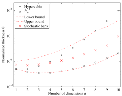
Figure 1: The normalized thickness $\theta$ as a function of the number of dimensions $d$ for a stochastic template bank in $\mathbb{E}^{d}$ (crosses). In addition, the lower and upper bounds for stochastic template banks are shown, derived from the known minimum and maximum possible normalized thickness values for the sphere packing problem Schürmann and Vallentin ; Conway and Sloane (1993) as described in the text. For comparison, also lattice placement algorithms (hyper-cubical and $A_{n}^{*}$) are displayed.

Extending Fig. 1 of HAS09, we are also able to compute the normalized thickness for a stochastic template bank for up to 10 dimensions. This calculation was only made possible owing to the significantly improved computational efficiency of the NCA algorithm presented in this work. Due to computational limitations, in HAS09 the results for only up to 4 dimensions have been reported. For dimensions higher than 3, the stochastic bank increasingly improves in performance compared to the simple hyper-cubical lattice. Though the stochastic bank with complete coverage appears to be less efficient than the $A_{n}^{*}$ lattice. However, any such lattice coverings and constructions algorithms are only defined for the cases of flat parameter spaces. In contrast, the stochastic template bank generation with the NCA in principle can be done for any parameter space and thus can prove especially useful for non-flat parameter spaces.

When generating a stochastic template bank, it is useful to define the covering fraction $f\in[0,1]$, which denotes the faction of $V_{M}$ that is covered by the union of all template volumes. As HAS09 note, $f$ is also related to the computational complexity to populate the stochastic template bank, because the expected number of candidate templates required to accept one template to the bank increases as $1/(1-f)$.

III The neighboring cell algorithm

III.1 Key elements and requirements of the NCA

In the following we describe the key elements and basic requirements of the NCA in order to efficiently generate a stochastic template bank:

1. The entire parameter space is divided into non-overlapping sub-volumes that we denote as cells. For simplicity and ease of computing, we employ hyper-cubical cells in a Cartesian coordinate system. Any other regular or non-regular structure is also possible.

2. Each cell must be uniquely indexed.

3. Generally, two cells are neighbors if at least one common parameter-space point of one cell and a template covering volume exists where the template lies inside the other cell. In Cartesian coordinates and hyper-cubical cells neighboring cells have at least one border point in common. For a given cell index, the indices of the neighboring cells can be computed.

4. Each template must be uniquely indexed.

5. Each template index is mapped to a cell index that labels the cell in which the template position lies.

6. Given a parameter-space position of a template, the index of its enclosing cell is readily computed by a hashing algorithm. For a hyper-cubical cell lattice this is accomplished by a fast rounding or truncating operation on the parameter values of the template position.

7. The parameter-space covered by a template only overlaps with the space of the enclosing cell and the neighboring cells. It must not overlap with the space of non-neighboring cells. This is ensured by either choosing a small enough covering radius of the templates, or by designing the cells sufficiently large.

The NCA requires two different tables to be kept in memory. First, the template table, which stores the indices and the parameter-space positions of all templates. Second, the cell table, which contains all cell indices and the list of template indices of template positions lying within each cell. Figure 2 shows a simplified example for the contents of the cell table.

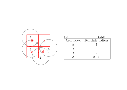
Figure 2: Exemplary illustration of the cell table, which contains all cell indices and the list of template indices of template positions lying within each cell. Shown on the left are four templates (black circles) labeled by indices $\{1,2,3,4\}$. The cells (red boxes) are labeled by the indices $\{a,b,c,d\}$.

III.2 Stochastic template placement with the NCA

The following procedure describes how to generate a stochastic template bank with covering fraction $f$ using the NCA. Starting with an empty template bank, the process for adding new templates to the bank is as follows:

1. Draw a random point in $M$ as a candidate template for addition to the bank.

2. Determine the cell the candidate template falls into by calculating its cell index $i_{\rm C}$.

3. Compute the cell indices of all neighboring cells. We refer to the resulting list of neighboring cells including the enclosing cell $i_{\rm C}$ as the neighboring-cell (NC) list. Note that a cell that is a $d$-dimensional hypercube, has ($3^{d}-1$) neighboring cells.

4. Sort the NC list in order of increasing distance. Start with $i_{\rm C}$ and proceed with the closest neighboring cells. The distance between two cells is defined as the distance between the centers of the cells. For illustrative purposes, Fig. 3 shows an example for the NC list.

5. Retrieve a list of all template indices associated with the cells of the NC list.

6. For all retrieved template indices obtain the template positions from the template table.

7. Compute the distance between the candidate template and every other template position of those obtained in the previous step. Start with the templates located in cells nearest to cell $i_{\rm C}$. If all computed distances exceed the predefined covering radius, accept this candidate template as a new template and assign it the next consecutive template index.

8. If the candidate template has been accepted, update the template table: Append the position of the accepted candidate template to the template table. Also update the cell table: Append the template index to the list of template indices pertaining to the cell $i_{\rm C}$ in the cell table.

9. Repeat this procedure starting from step (1) until the covering fraction $f$ has reached the desired value.

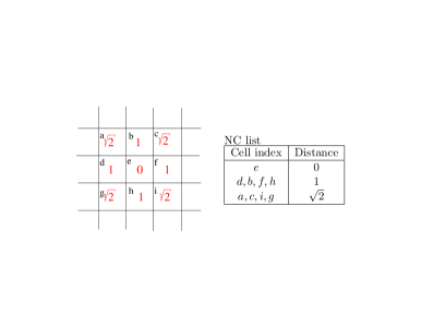
Figure 3: Schematic illustration of the distances between neighboring cells of the NC list. The letters $\{a,b,c,d,e,f,g,h,i\}$ represent the cell indices. The numbers shown are the distances from the center of the cell labeled by $e$ to each center of the other cells shown. For maximum efficiency, the NC list is sorted by increasing order of this distance as explained in the text.

III.3 Computational cost improvements from the NCA

A major drawback of the standard stochastic template bank algorithm by HAS09 is the computational complexity which can become even prohibitive. This is because for each new candidate template its distance to every other template of the existing bank has to be computed and compared to the covering radius before eventual acceptance to the bank. With increasing covering fraction the probability of accepting a candidate template decreases. At the beginning, when the covering fraction substantially less than one, the estimated computational cost for accepting a new candidate template increases approximately quadratically with the number of templates in the bank, since almost no templates are rejected. For covering fractions closer to one the computational cost increases much faster than quadratically with the number of templates in the bank, because the rejection of candidate templates dominates. It is this prohibitive computing cost that can quickly render the acceptance of new templates computationally intractable in the standard stochastic template bank algorithm.

In order to demonstrate the significant computational efficiency improvement of the NCA over the standard algorithm, we consider the generation of a stochastic template bank in a 3-dimensional Euclidean space with periodic boundary conditions, where each coordinate lies within $[0,1]$. The template covering radius $r$ is chosen, such that the bank contains $3.5$ million templates at a covering fraction of $f=99.9\%$, which is given by $r=1/180$ and implies a normalized thickness of about $0.6$. To compare the computational costs of both algorithms when constructing this bank, we count the total number of distance computations required in either case. Figure 4 shows the results of this comparison study. With the NCA, the total number of distance computations is massively reduced and about five orders of magnitude lower compared to the standard algorithm. This gain factor is not surprising but straightforward to understand: It is simply the ratio of the total volume of the considered parameter space to the volume enclosed by a single cell and its $(3^{3}-1)$ neighboring cells, which gives $180^{3}/27\approx 2\times 10^{5}$ in this example.

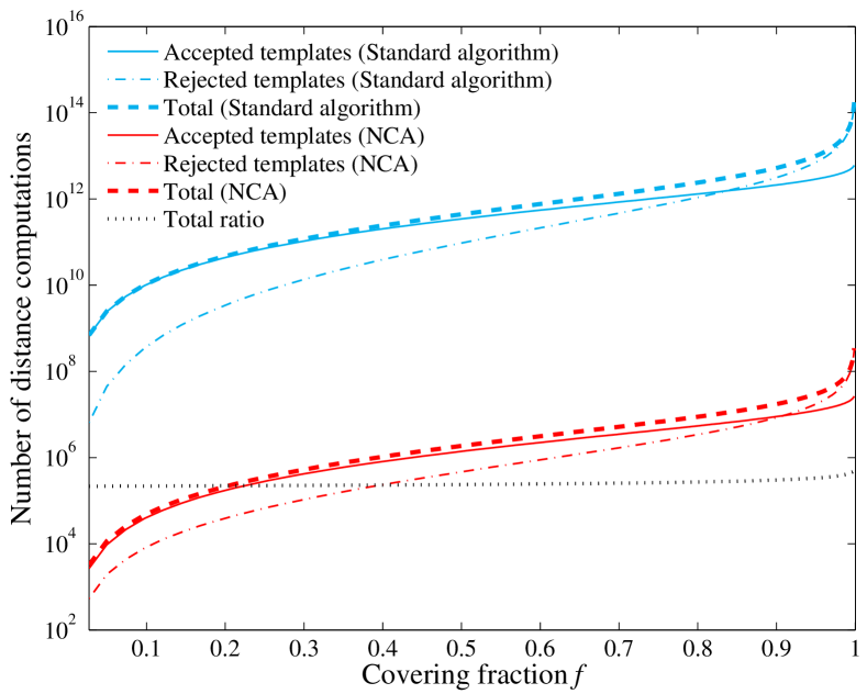
Figure 4: Comparison the computing cost (measured by the number of distance computations) between the standard algorithm and the NCA to generate a stochastic template bank in $\mathbb{E}^{3}$. Shown as a function of the covering fraction $f$ for each method is the number of distance computations for candidate templates that have been accepted (thin solid) and rejected (thin dotted-dashed), as well as the total number (thick dashed). With the NCA, the total number of distance computations is massively reduced, by more than five orders of magnitude as shown by the dotted curve.

Figure 4 also shows the shares in the total number of distance computations separately for rejected and accepted candidate templates. As can be seen, at the beginning for low covering fractions, the computing cost is dominated by the distance computations for accepted candidate templates. As the template bank is getting more populated at higher covering fractions, a turnover occurs, where the computing cost starts being dominated by the distance computations due to rejections and increases much more rapidly. As can be seen, compared to the standard algorithm for the NCA this turnover takes place at a larger covering fraction. This is mainly due to the NCA’s much more efficient rejection of candidate templates, as described in the following.

Sorting the NC list of neighboring cells is crucial for the efficiency of the NCA, specifically in view rejecting candidate templates. This sorting [done in step (4) in Sec. III.3 above] as part of the NCA stochastic template bank generation considerably reduces the average number of distance computations needed before a candidate template is eventually rejected. As illustrated in Fig. 3, this is obvious, because on average the overlapping volume of the candidate template is highest with the own cell and decreases for the neighboring cells. Therefore, the probability for rejecting a candidate template is the highest when comparing to those templates located in the same cell. Hence, the sorting of the NC list by distance of step (4) can also be seen as sorting by decreasing order of probability of rejection, which thus overall minimizes the average number of distance computations. This is also seen in that the gain factor between the NCA and the standard scheme (dotted curve in Fig. 4) is mostly constant but increases for covering fractions closer to one, where the rejections of candidate templates dominate.

With higher dimensions this effect gains even more importance, because the number of neighboring cells increases exponentially with dimension. For example, if $d=3$ the number of considered cells is $3^{3}=27$. Without sorting and a cell addressing scheme as shown in Fig. 3, the cell containing the candidate would be on average the $(3^{3}+1)/2=14$th cell considered. After sorting, the cell enclosing the template candidate is considered first. Hence, this sorting can decrease the number of distance computations by a factor almost $14$. Whereas, if $d=10$ the number of considered cells is $3^{10}=59049$. The cell containing the candidate in absence of sorting would be the $(3^{10}+1)/2=29525$th cell considered. Therefore, sorting the NC list can decrease the number of distance computations in $d=10$ by almost $30\,000$! This efficiency gain has greatest importance for covering fractions nearing one, where the majority of candidate templates is rejected (see Fig. 4).

The NCA also significantly facilitates evaluating the covering fraction at the different stages of the stochastic bank generation. The covering fraction is typically obtained via Monte Carlo integration using a sufficient number of sample points (as also done in HAS09). The standard algorithm by HAS09 has to compute the distances between a sample point and all templates in the bank, which is inefficient. The NCA instead readily can provide a list of the subset of templates closest to a given sample point, and only the distances to those are computed. This way, wasteful distance computations for templates far away from the sample-point location are avoided, as those templates will obviously have no overlap with the sample point.

IV Increasing the covering fraction by shifting templates

The generation of stochastic template banks with covering fractions nearing unity can become quickly computationally prohibitive (cf. Fig. 4). This is due to the enormous number of candidate templates to be tested before a new template is accepted to the bank. Here, we present a possible and efficient alternative solution to this problem. The idea is to first generate a stochastic template bank with initially smaller covering fraction and then increase the covered space by only shifting the positions of the templates, instead of adding new ones.

IV.1 Barycentric template shifts

In what follows, we describe a scheme to effectively shift the templates in the bank with the goal of increasing the overall covering fraction. One such shift optimization stage begins with the first template in bank:

1. Determine a set of points uniformly distributed on the boundary of the covering volume of the template. Note that the boundary of a covering volume is the set of points which have distance $r$ (the covering radius) to the template position.

2. Check whether each of these points is covered or not by another template. If covered the boundary point gets the zero weight, otherwise a weight of unity. In case a boundary point lies outside of the relevant parameter space this point gets also zero weight.

3. From the set of boundary points with unit weight, calculate the barycenter of these points.

4. If the distance between the template position and the barycenter is smaller then a certain maximum distance $\epsilon$, the template is moved to coincide with the barycenter. If the distance is larger than $\epsilon$, the template position moved in the direction of the barycenter by only $\epsilon$.

5. Carry out the procedure starting from step (1) for the next template until done for all templates in the bank.

The above scheme (forming a single optimization stage) is to be repeated until the covering fraction does not increase anymore (or any other terminating condition is met). In general, step (4) will increase the fraction of covered parameter space. However, it might also happen that occasionally a template is shifted towards an existing template, leading to an undesired newly created overlap. To mitigate this effect, we therefore recommend to set the maximum shift distance $\epsilon$ at a fraction of $r$. Within this work we found that choosing a maximum shift of $\epsilon=0.05\,r$ provides overall satisfactory results.

IV.2 Choice of boundary points and computing cost

The actual number of boundary points used is a tradeoff between accuracy of the barycentric shift and computational efficiency. As a lower bound, to be able to shift the template position into any direction in a $d$-dimensional parameter space, the minimum number of points should is $2d$. More boundary points will improve the accuracy of the shift, but also decrease the computational efficiency of a single optimization stage. While a more detailed study of these aspects is beyond the scope of this paper, one scheme we found to work sufficiently well for our purposes is choosing twice as many boundary points as there are neighboring cells, i.e. $2\times(3^{d}-1)$ points.

One way to place the set of boundary points as required in step (1) is the following approach, first presented in von Neumann (1951); Cook (1957). In a $d$-dimensional Euclidean space with spherical template volumes, a uniformly distributed set of boundary points can be obtained by placing random points uniformly into the enveloping hyper-cubical box. As illustrated in Fig. 5, then all points lying outside of the sphere are discarded and those inside the sphere are projected onto the boundary to provide the desired set of boundary points.

The computational cost of this optimization scheme is again dominated by the number of distance computations. In this method, the number of needed distance computations $D$ is simply the product $D=N_{O}\times N_{B}\times N_{S}\times N\times$, where $N_{O}$ is the number of optimization stages, $N_{B}$ is the number of boundary points, $N_{S}$ is the average number of templates in the considered within the subvolume of the neighboring cells, and $N$ is the total number of templates. As mentioned above, $N_{B}$ can be taken as $2\times(3^{d}-1)$. Moreover, $N_{S}$ is estimated as the normalized thickness $\theta$ times the number of neighboring cells plus the own cell giving $3^{d}$. The value of $N_{O}$ depends on the used shifting method, while typically we reached convergence after $N_{O}=20$ stages. Thus, for example in three dimensions, the number of required distance computations using the normalized thickness of the optimal covering is $D=20\times 26\times 9.8\times N\approx 10200\times N$. It is worth noting that since the computational cost is only linear in the total number of templates $N$, this proposed scheme is feasible also for a relatively large template banks.

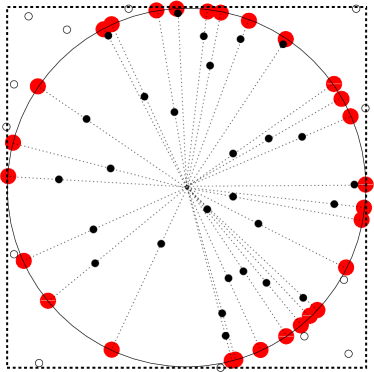
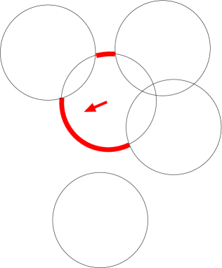
Figure 5: Schematic illustration of the barycentric template shifts to increase the covering fraction. Left: Illustration of the generation of the boundary points. In the enclosing cube around the sphere random points are placed uniformly. The points falling outside of the template volume (small hollow points) are ignored. The points are inside the sphere (small filled black points) they are projected onto the boundary of the template volume, providing the boundary points. Right: The thick red lines shows points on the boundary of a template covering volume that have weight one. These points are not covered by any neighboring template. All other boundary points get the weight zero. Using these weights we can compute the barycenter of the boundary points. The arrow points from the current position of the template to the center of mass of the unit-weight (red thick) boundary points. The resulting shift of the template position towards this barycenter thus increases the covering fraction.

Figure 6: Illustration of different optimization stages of a $2$-dimensional stochastic template bank in Euclidean space with a normalized thickness of $0.38$. The individual panels are: (a) Unoptimized template bank that has a covering faction of $0.89$; (b) Template bank after $12$ optimization stages (template shifting) that has a covering fraction of $0.978$; (c) Template bank after $120$ optimization stages that has a covering fraction of $0.995$.

IV.3 Performance demonstration

Figure 6 illustrates the optimization effect from barycentric template shifting for a stochastic template bank in a 2-dimensional Euclidean space. Here, we repeatedly apply the template shifting optimization to the bank. With an increasing number of such optimization steps it becomes apparent that the template bank approaches an $A_{2}^{*}$ lattice structure. Since in this simple example the chosen parameter space is quadratic with periodic boundary conditions, a perfect $A_{2}^{*}$ cannot be obtained, therefore defects are expected. This can be avoided by choosing an appropriate size of the parameter space. Such an example choice for length $l$ and width $w$ in 2 dimensions would be $l/w=\sqrt{3}/2$ and a covering radius of the templates that is an integer fraction of $w/\sqrt{3}$.

To evaluate the performance of the template shifting optimization method, we study the increase in covering fraction $f$. Again, for simplicity we consider the Euclidean space $\mathbb{E}^{d}$ with up to $d=8$ dimensions. For all dimensions, we choose again $r=1$ template shifts are limited to at most $5\%$ of the covering radius, so that $\epsilon=0.05$. The resulting reduction of non-covered parameter space (i.e. increasing $f$) is presented in Fig. 7. As can be seen from the figure, after a few optimization steps of collective template shifting the non-covered fraction of space (that is $1-f$) can be significantly reduced. Ultimately after a sufficient number of optimization steps the fraction of non-covered can be decreased by two orders of magnitude compared to the standard stochastic template bank (corresponding to zero optimization steps). Recall that this achievement has been made without the addition of any extra templates to the bank. Further improvements could eventually be made by varying or adapting $\epsilon$ during the run time, achieving a faster convergence or better covering. Similarly, replacing the barycentric “fixed-size” template shift with some simplex or gradient driven downhill method could better take into account the overlapping volume of nearby templates and enable even more effective template shifts.

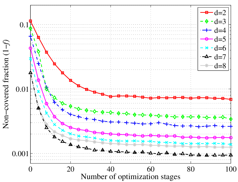
Figure 7: The decreasing fraction of non-covered parameter space (that is just $1-f$) with the number of optimization stages. At each stage, the barycentric template shifting method is applied using maximum shifts of $\epsilon=0.05$. The different curves are for Euclidean spaces $\mathbb{E}^{d}$ with dimensions from $d=2$ up to $d=8$, using periodic boundary conditions and a template covering radius $r=1$.

V Further examples to test the NCA

For maximum efficiency of the NCA, the cells should be constructed to adapt to the parameter space structure, e.g. following the local metric approximation. In particular for curved parameter spaces the cell construction and the determination of neighboring cells requires care and can be difficult, in particular in higher dimensions since the number of neighboring cells grows exponentially with the dimension. However, when it is not possible to determine the exact set of neighboring cells it always is save to just use a somewhat larger set of cells (that is simpler to determine, but does include cells which are not strict neighbors). This would only slightly reduce the performance since distances between more templates have to be computed than actually necessary. On the other hand, missing neighboring cells could lead to a more severe issue, since this would lead to over-covering of templates in the regions of the missed neighboring cells. In what follows, we show further exemplary applications of the NCA, one related to the choice of coordinates on parameter space, and one for a parameter space that is curved.

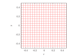
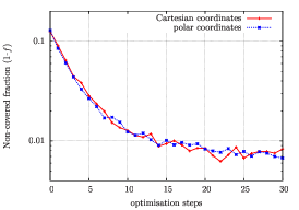
Figure 8: Example application of the NCA for Cartesian and polar coordinates. The individual panels are: (b) Schematic illustration of cell construction when using Cartesian coordinates. (b) Schematic illustration of cell construction when using polar coordinates. (c) Comparison of the non-covered fraction $(1-f)$ for Cartesian and polar coordinates. In this comparison, we employed a template covering radius of $r=0.01$ and a total number of templates $N=4000$. To determine the non-covered fraction we used $20000$ Monte Carlo points.

V.1 Choice of coordinates

In principle, the NCA and the optimization are independent of the choice of the coordinates. This is demonstrated in the following example. Figure 8 illustrates the parameter space splitting (cell construction) for the NCA in Cartesian $(x,y)$ and in polar coordinates $(\rho,\phi)$. The coordinate transformation is given by $x=\rho\cos\phi$, $y=\rho\sin\phi$ and the distance is computed as $d=\left(x^{2}+y^{2}\right)^{1/2}$. It is obvious that in polar coordinates the cells are obtained by dividing the parameter space into rings of width $r$, where $r$ is the covering fraction of the templates. Each ring is fragmented so that a template covering volume reaches only the neighboring cells and never the cells beyond. The neighboring cells are the adjacent cells in the same ring and any cell in the adjacent rings which can be “reached” by the covering volume of any template in lying inside the considered cell. This can also include cells which have no common boundary points with the considered cell. Finally, the results of from applying the NCA for both choices of coordinates are also presented in Fig. 8, showing that the non-covered fraction as a function of the number optimization stages (using barycentric shifts, see Sec. IV), is effectively the same for both choices of coordinates.

V.2 Curved parameter space

To illustrate the applicability of the NCA for a curved (i.e. non-flat) parameter space, we consider generating a stochastic template bank on the sphere – an example that was also used in HAS09. A sphere here means a set of points with the same distance to a center point, where unit distance is used for simplicity in the present example. Thus the length element is defined as $dl=d\theta+d\phi\cos\theta$ were $-\pi/2\leq\theta\leq\pi/2$ and $0\leq\phi<2\pi$. The cells in parameter space are constructed, using uniform spacings in the $\theta$-direction. The cell sizes $\Delta\phi$ in the $\phi$ direction should depend on $\theta$. Because the cell construction should be such that the covering volumes of templates overlap only with neighboring cells, we choose $\Delta\phi=r/\cos\theta_{b}$, where $\theta_{b}$ minimizes $\cos\theta$ within this cell. Making $\Delta\phi$ smaller would result in template volumes which could reach into non-neighboring cells. In this example, determining the neighboring cells works similar as described above for polar coordinates. For a given $\theta$ one has to find all cells which could have an overlap with any template inside the considered cell. In Fig. 9, the cell construction in parameter space is displayed, along with the stochastic template generated by the NCA, as well as the optimized template bank using the barycentric shift method introduced in Sec. IV.

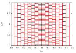
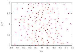
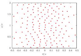
Figure 9: Example application of the NCA to place templates on the sphere, parameterized by the polar angle $\theta$ and the azimuth angle $\phi$. Here $\theta=0$ denotes the equatorial plane. The individual panels are: (a) Illustration of cell construction in parameter space. (b) Stochastic template bank from the NCA containing $150$ templates and having a covering fraction of $f=0.858$. (c) Optimized template bank by the NCA with an improved covering fraction of $f=0.984$ for the same number of templates. The template covering radius has been chosen as $r=0.18$ in this example.

VI Generalization of the NCA

In this section, we describe a conceptual idea how to generalize the NCA for application even to arbitrarily “ill-behaved” parameter spaces. In general, the smaller the average number of templates per cell the smaller the number of required distance computations needed by the NCA. However, for certain parameter spaces, the shape or the size of the template volumes might be unknown or vary strongly across the space. This might represent a non-negligible problem in order to meet requirement (7) of Sec. III.1, as one has to choose the size of the cells to be sufficiently large. It may even lead to extreme situations, where the efficiency gain from the NCA can melt away.

To address this problem of ill-behaved parameter spaces, we suggest the following strategy. To begin with, set up the cells with a smaller size that actually violates the requirement (7) of Sec. III.1. Then notice that in some regions of parameter space, a template overlaps with many cells and not only with neighboring ones. Therefore, one can combine these cells to form a single virtual cell. Those virtual cells then again meet all requirements for the NCA as outlined in Sec. III.1. This basic idea is illustrated in Fig. 10. To combine cells the following recipe is proposed:

• Start with the first cell and place a template inside this cell at a random position. Form the first virtual cell labeled $A$, which contains that first cell.

• Consider the next cell and place a second template inside. If the first and second templates are too close to each other, the second cell also belongs to the same virtual cell $A$. In this case the second template can be discarded and the first template is the representing template for the virtual cell $A$. On the other hand, if the distance between the two templates is large enough, the second cell forms another virtual cell labeled $B$, containing the second cell. In this case, the first template represents $A$ and the second represents $B$.

• Continue this scheme subsequently for all other cells and test whether the considered cell belongs to one of the existing virtual cells. If not, the considered cells forms a new virtual cell.

• Keep a list in memory which maps all cells to their virtual cells.

• A virtual cell inherits the neighbors of its containing cells. Note that if an inherited neighboring cell is also a part of the same virtual cell, this cell has to be removed from the list of neighbors.

This procedure will create a map of virtual cells which cover the entire parameter space. While not guaranteed to generate the smallest possible virtual cells meeting condition (7) in Sec. III.1, this method is a viable solution and more flexible than the basic version of the NCA described in Sec. III. To check whether a specific point in parameter space is covered by one of the templates, one proceeds as follows:

• Compute the cell index for the parameter-space point.

• Map the cell to the virtual cell and read out the indices for the neighbored virtual cells.

• Collect all templates from the template lists of the own and the neighbored virtual cells and compute all distances between the examined point and these templates.

• If one of the computed distances is smaller than the desired covering radius, the point is covered.

For illustrative purposes, Fig. 10 shows a simplified example to which above method is applied.

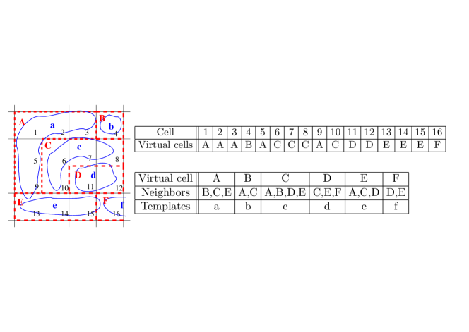
Figure 10: Illustration of NCA generalization by combining cells to form virtual cells for arbitrary parameter-space structures. The cell indices are indicated by Arabic numbers. The virtual-cell indices are labeled with red capital letters. The templates are denoted by lower-case letters. The left panel illustrates schematically the borders of the templates, cells, and virtual cells. The right top table shows a table for the corresponding cell to virtual-cell mapping. The right bottom table presents a table that lists the neighbors of the virtual cells.

VII Conclusions

This paper presents a neighboring cell algorithm (in short NCA) to efficiently construct stochastic template banks covering multidimensional parameter spaces. A core improvement from the NCA is the dramatic reduction in the number distance computations, achieved by dividing the parameter space into separate cells (neighboring cells). For any point in parameter space we exploit an efficient hashing technique to obtain the index of the enclosing cell (and thus the parameters of its neighboring templates). This way, to test if a new candidate template should be added to the bank, only templates located within the own and neighboring cells have to be considered. Previous methods Harry et al. (2009); Babak (2008) required comparison (i.e. distance computation) with all templates already in the bank and thus were considerably more computational expensive and eventually prohibitive for large (or also high-dimensional) parameter spaces. We have demonstrated that compared to the standard stochastic template bank algorithm, the NCA can reduce the number of distance computations in a $3$-dimensional Euclidean space by about five orders of magnitude. In addition, based on the NCA we have described a new method to significantly increase the covered fraction of parameter space, solely through systematic shifts of the template positions – without adding further templates to the bank.

The NCA is guaranteed to work efficiently if the average number of templates per neighboring cell is small. For cases, where the shape and size of the template volumes vary drastically across parameter space, this can be eventually become difficult to achieve. To address this problem, we have presented a method to generalize the NCA by combining many neighboring cells to form so-called virtual neighboring cells. The arrangement of the virtual neighboring cells can adapt adequately to the local parameter-space structure (the shape of the covered template volumes).

Apart from generating template banks, it should be pointed out that the NCA can also be used to efficiently validate the produced bank. This is usually done by searching synthetic data sets containing simulated signals and determining the resulting minimum mismatch in each case. The NCA considerably accelerates this process by avoiding the need of having to the search the entire template bank for every simulated-signal data set. Instead, for any given parameter-space position of a simulated signal, the NCA can readily provide the subset of templates closest to the signal position, which are the only ones relevant. Templates further away from the signal location are irrelevant, since those will obviously have high mismatch with the signal. Iterating this procedure for a large number of simulated signals across the parameter space, gives rise to a mismatch histogram to validate the efficiency of the entire template bank.

The NCA, including the generalized version presented, has applicability in different areas of astronomy. For example in gravitational-wave searches for inspiral or continuous-wave sources Babak et al. (2012); Aasi et al. (2012), exploiting the NCA can potentially offer great efficiency gains. In the field of gamma-ray pulsar astronomy, the NCA has already been successfully used to construct an optimized stochastic template bank to search data from the Fermi Large Area Telescope for a pulsar binary system Pletsch et al. (2012). Further details involved and results from these applications of the NCA are subject to forthcoming work.

Directions for a future work also include technical and methodological improvements. In this work, we implemented the NCA in a parallel algorithm using OpenMP and executed the program on a single system. However, it might be worthwhile to port to an MPI version which runs on many compute nodes or use remote databases to hold the template and the cell table. The practicability of such algorithms has to be investigated, particularly since random access on the entire table ranges is required. Finally, a further improvement of the optimization method could be achieved by replacing the barycentric “fixed-size” template shift with some simplex or gradient driven downhill method. This approach would better take into account the overlapping volume of nearby templates and enable even more effective template shifts.

VIII Acknowledgments

We thank Bruce Allen for discussions of the basic ideas behind this work and for pointing out to us open questions concerning the convergence behavior of stochastic template banks. We are grateful for fruitful discussions with Reinhard Prix, Chris Messenger, Oliver Bock and Carsten Aulbert. We thank Benjamin Knispel and Gian Mario Manca for discussing possible further applications and some future directions of this work. The concept of hash algorithms in numerical physics we owe to Bogdan Damski. This work was supported by the Max-Planck-Gesellschaft (MPG), as well as by the Deutsche Forschungsgemeinschaft (DFG) through an Emmy Noether research grant PL 710/1-1 (PI: Holger J. Pletsch).

References

- Sathyaprakash and Dhurandhar (1991) B. S. Sathyaprakash and S. V. Dhurandhar, Phys. Rev. D 44, 3819 (1991).
- Dhurandhar and Sathyaprakash (1994) S. V. Dhurandhar and B. S. Sathyaprakash, Phys. Rev. D 49, 1707 (1994).
- Cutler and Flanagan (1994) C. Cutler and E. E. Flanagan, Phys. Rev. D 49, 2658 (1994).
- Jaranowski and Królak (2005) P. Jaranowski and A. Królak, Living Reviews in Relativity 8, 3 (2005).
- Babak et al. (2012) S. Babak, et al. Phys. Rev. D 87, 024033 (2012).
- Aasi et al. (2012) J. Aasi, J. Abadie, B. P. Abbott, et al. (2012).
- Abbott et al. (2004) B. Abbott et al., Nuclear Instruments and Methods in Physics Research A 517, 154 (2004).
- Abramovici et al. (1992) A. Abramovici et al., Science 256, 325 (1992).
- Acernese et al. (2006) F. Acernese et al., Class. Quant. Grav. 23, 635 (2006).
- Gossler et al. (2002) S. Gossler et al., Class. Quant. Grav. 19, 1835 (2002).
- Willke et al. (2002) B. Willke et al., Class. Quant. Grav. 19, 1377 (2002).
- Takahashi et al. (2004) H. Takahashi et al. (TAMA Collaboration), Class. Quant. Grav. 21, 697 (2004).
- Danzmann and the LISA Study Team (1998) K. Danzmann and the LISA Study Team, Max-Planck-Institut für Quantenoptik, Report MPQ 21, 233 (1998).
- Knispel et al. (2010) B. Knispel et al., Science 329, 1305 (2010).
- Allen et al. (2013) B. Allen et al., The Astrophysical Journal 773, 91 (2013).
- Pletsch et al. (2012) H. J. Pletsch et al., Science 338, 1314 (2012).
- Helstrom (1968) C. W. Helstrom, Statistical Theroy of Signal Detection (Pergamon Press, 1968).
- Whalen (1971) A. D. Whalen, Detection of Signals in Noise (Academic Press, New York and London, 1971).
- Manca and Vallisneri (2010) G. M. Manca and M. Vallisneri, Phys. Rev. D 81, 024004 (2010).
- Conway and Sloane (1993) J. Conway and N. Sloane, Sphere Packings, Lattices and Groups (Springer-Verlag, New York, 1993).
- (21) A. Schürmann and F. Vallentin, Geometry of lattices and algorithms, http://www.math.uni-magdeburg.de/lattice_geometry/.
- Vallentin (2003) F. Vallentin, Ph.D. thesis, Technische Universität München, Zentrum Mathematik (2003).
- Messenger et al. (2009) C. Messenger, R. Prix, and M. A. Papa, Phys. Rev. D 79, 104017 (2009).
- Sobol (1967) I. M. Sobol, USSR computational mathematics and mathematical physics 7, 86 (1967).
- Sobol (1976) I. M. Sobol, USSR computational mathematics and mathematical physics 16, 236 (1976).
- Lampert (1988) J. P. Lampert, International Series of Numerical Mathematics 86, 273 (1988).
- Harry et al. (2009) I. W. Harry, B. Allen, and B. S. Sathyaprakash, Phys. Rev. D 80, 104014 (2009).
- Babak (2008) S. Babak, Class. Quant. Grav. 25 (2008).
- Allen and Shellard (1990) B. Allen and E. P. S. Shellard, Phys. Rev. Lett. 64, 119 (1990).
- Abbott et al. (2009) B. Abbott et al. (LIGO Scientific Collaboration), Phys. Rev. D 79, 022001 (2009).
- Balasubramanian et al. (1996) R. Balasubramanian, B. S. Sathyaprakash, and S. V. Dhurandhar, Phys. Rev. D 53, 3033 (1996).
- Owen (1996) B. J. Owen, Phys. Rev. D 53, 6749 (1996).
- von Neumann (1951) J. von Neumann, NBS Applied Mathematics Series 12, 36 (1951).
- Cook (1957) J. M. Cook, Mathematical Tables and Other Aids to Computation 11, 81 (1957).