Real-time flare detection in ground-based H$\alpha$ imaging at Kanzelhöhe Observatory

Abstract

Kanzelhöhe Observatory (KSO) regularly performs high-cadence full-disk imaging of the solar chromosphere in the H$\alpha$ and Ca ii K spectral lines as well as the solar photosphere in white-light. In the frame of ESA’s Space Situational Awareness (SSA) programme, a new system for real-time H$\alpha$ data provision and automatic flare detection was developed at KSO. The data and events detected are published in near real-time at ESA’s SSA Space Weather portal (http://swe.ssa.esa.int/web/guest/kso-federated). In this paper, we describe the H$\alpha$ instrument, the image recognition algorithms developed, the implementation into the KSO H$\alpha$ observing system and present the evaluation results of the real-time data provision and flare detection for a period of five months. The H$\alpha$ data provision worked in $99.96$% of the images, with a mean time lag between image recording and online provision of 4 s. Within the given criteria for the automatic image recognition system (at least three H$\alpha$ images are needed for a positive detection), all flares with an area $\geq$50 micro-hemispheres and located within $60^{\circ}$ of the Sun’s center that occurred during the KSO observing times were detected, in total a number of 87 events. The automatically determined flare importance and brightness classes were correct in $\sim$85%. The mean flare positions in heliographic longitude and latitude were correct within $\sim$1^∘. The median of the absolute differences for the flare start times and peak times from the automatic detections in comparison to the official NOAA (and KSO) visual flare reports were 3 min (1 min).

iint iiint

1 Introduction

Introduction

Solar flares are sudden enhancements of radiation in localized regions on the Sun. The radiation enhancements are most prominent at short (EUV, X-rays) and long (radio) wavelengths, with only minor changes in the optical continuum emission. However, flares are well observed in strong absorption lines in the optical part of the spectrum, most prominently in the H$\alpha$ Balmer line of neutral hydrogen at $\lambda=656.3$ nm. Flares typically occur within active regions of complex magnetic configuration (e.g. Sammis, Tang, and Zirin, 2000). They are the result of an impulsive release of magnetic energy previously stored in non-potential coronal magnetic fields via flux emergence and surface flows. The released energy is converted into the acceleration of high-energy particles (Wiegelmann, Thalmann, and Solanki, 2014), heating of the solar plasma and mass motions (e.g., reviews by Priest and Forbes, 2002; Benz, 2008; Fletcher et al., 2011). Flares may or may not occur in association with coronal mass ejections (CMEs). However, the association rate is a strongly increasing function of the flare importance, and in the strongest and most geo-effective events typically both occur together (Yashiro et al., 2006).

CMEs, flares and solar energetic particles (SEPs), which are accelerated either promptly by the flare or by the interplanetary shock driven ahead of fast CMEs, are the main sources for severe space weather disturbances at Earth. CMEs are only very limited accessible to observations from ground, due to their faint appearance and the stray light in the Earth atmosphere. They are best tracked in white-light images recorded from coronagraphs on space-based observatories. Flares are regularly observed at X-ray and (E)UV wavelengths from satellites, but they are also well observed from ground-based observatories in the H$\alpha$ spectral line.

Besides regular visual detection, reporting and classification of solar H$\alpha$ flares by a network of observing stations distributed over the globe, and collection at NOAA’s National Geophysical Data Center (NGDC), there are also recent efforts to develop automatic flare detection routines. The detection methods range from comparatively simple image recognition methods based on intensity variation derived from running difference images (Piazzesi et al., 2012), region-growing and edge-based techniques (Veronig et al., 2000; Caballero and Aranda, 2013) to more complex algorithms using machine learning (Qahwaji, Ahmed, and Colak, 2010, Ahmed et al., 2013) or support vector machine classifiers (Qu et al., 2003). These methods have been applied to space-borne image sequences in the EUV and soft X-ray range (e.g, Qahwaji, Ahmed, and Colak, 2010; Bonte et al., 2013; Caballero and Aranda, 2013), but also to ground-based H$\alpha$ filtergrams (e.g., Veronig et al., 2000; Henney et al., 2011; Piazzesi et al., 2012; Kirk et al., 2013).

The flare classification system used in this paper is based on the H$\alpha$ flare importance classification (Švestka, 1966). Figure xray_opt_fig shows the relation between the optical H$\alpha$ flare importance class and the X-ray flare class from the Geostationary Operational Environmental Satellites (GOES). The scatter plot contains all flares observed at KSO during the period 1/1975 - 10/2014 that were located within 60$\deg$ from the central meridian. The associated GOES X-ray flares were automatically identified by the following criteria: the soft X-ray and H$\alpha$ flare peak times are within 10 min and the heliographic positions are within 10$\deg$. Figure xray_opt_fig reveals a high correlation between the H$\alpha$ importance class (defined by the chromospheric flare area; cf. Table tab:flares1) and the GOES X-ray class (defined by the peak flux in the 1-8 Å channel). In total the set comprises 2832 flares with the following distributions among the classes (H$\alpha$ importance: 81.2% subflares, 15.4% importance 1, 2.6% importance 2 and 0.8% importance 3 and 4; GOES X-ray class: 86.0% B and C, 12.5% M and 1.5% X-class flares).

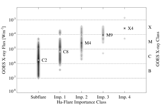
Figure 1.: GOES X-ray flares plotted against H$\alpha$ flares observed at KSO. The dark background represents the density of data points, the stars indicate the mean of the logarithmic X-ray flare classxray˙opt˙fig

Space-based data have the advantage that there are no atmospheric disturbances (seeing, clouds) degrading the image quality, but there is a delay in the data availability related to the data downlink. Ground-based data have the advantage that the data are immediately available for further processing, and can thus be efficiently used for the real-time detection and alerting of transient events such as solar flares in the frame of a space weather alerting system - however, with the drawback that the image sequences may suffer from data gaps and bad seeing conditions causing varying image quality. These circumstances have to be accounted for by the image recognition algorithms applied.

In this paper, we present an automatic image recognition method that was developed for the real-time detection and classification of solar flares and filament eruptions in ground-based H$\alpha$ imagery. The algorithms have been implemented into the H$\alpha$ observing system at Kanzelhöhe Observatory (KSO), in order to immediately process the recorded images and to provide the outcome in almost real-time. This activity was performed in the frame of the space weather segment of ESA’s Space Situational Awareness (SSA) programme, and the real-time H$\alpha$ data and detection results are provided online at http://swe.ssa.esa.int/web/guest/kso-federated. In this paper, we concentrate on the automatic flare detection and classification system, which was implemented in the KSO observing system in June 2013, and present the evaluation of the system for a five month period. The automatic detection of filaments and filament eruptions will be presented in a subsequent study, as the method is still under improvement (first results are shown in Pötzi et al., 2014).

The paper is structured as follows. In Sect. 2, we describe the KSO solar instruments and observations. In Sect. 3, we outline the image recognition algorithms developed to automatically identify solar flares in H$\alpha$ images, and to follow their evolution (in terms of location, size, intensity enhancement and classification). Sect. 4 outlines how the real-time detection and alerting was implemented in the KSO observing system. In Sect. 5, the outcome of the real-time flare detection system is evaluated for a test period of five months from end of June to November 2013. In Sect. 6, we discuss the performance of the system.

2 KSO instrumentation and observations

Instrum

Kanzelhöhe Observatory for Solar and Environmental Research (KSO; http://kso.ac.at) is operated throughout the year at a mountain ridge in southern Austria near Villach (N 46^∘40.7’, 13^∘54.1’, altitude 1526 m). The site allows solar observations for about 300 days a year, typically 1400 hours of observations. KSO regularly performs high-cadence full-disk observations of the Sun in the H$\alpha$ spectral line (Otruba and Pötzi, 2003), the Ca ii K spectral line (Hirtenfellner-Polanec et al., 2011), and in white-light (Otruba, Freislich, and Hanslmeier, 2008). Figure sample_kso_fig shows an exemplary set of simultaneous KSO imagery in H$\alpha$, Ca ii K and white-light recorded on January 6, 2014. All data are publicly available via the online KSO data archive at http://kanzelhohe.uni-graz.at/ (Pötzi, Hirtenfellner-Polanec, and Temmer, 2013).

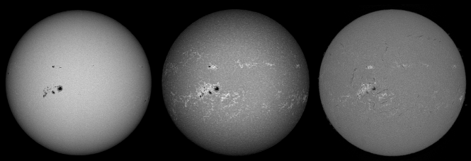
Figure 2.: Solar full-disk observations in white-light (left), Ca ii K (middle) and H$\alpha$ (right) recorded at Kanzelhöhe Observatory on January 6, 2014. sample˙kso˙fig

The observations are carried out by the KSO observing team during 7 days a week, basically from sunrise to sunset if the local weather conditions permit. All instruments for solar observations are mounted on the KSO surveillance telescope, which comprises four refractors on a common parallactic mounting (Figure telescope_fig). The KSO H$\alpha$ telescope is a refractor with an aperture ratio number of d/f = 100/2000 and a Lyot band-pass filter centered at the H$\alpha$ spectral line ($\lambda=656.3$ nm) with a Full-Width-at-Half-Maximum (FWHM) of 0.07 nm. For thermal protection an interference filter with an FWHM of 10 nm is in the light path. The Lyot filter can be tuned by turning the polarizers in narrow boundaries with little degradation of the filter characteristics. A beam splitter allows the application of two detectors at the same time. Currently, the observations are solely carried out in the center of the H$\alpha$ line.

The CCD camera of the H$\alpha$ image acquisition system is a Pulnix TM-4200GE with 2048 $\times$ 2048 Pixels and a Gigabit Ethernet interface. A frame rate of 7 images per second permits the application of frame selection (Roggemann et al., 1994; Shine et al., 1995) to benefit from moments of good seeing. The image depth of the CCD camera is 12 bit, which allows observing the quiet Sun and flares simultaneously without overexposing the flare regions. In order to have good counts statistics under varying seeing conditions and to avoid saturation effects in strong flares, an automatic exposure control system is in place; the automatically controlled exposure time lies in the range 2.5 to 25 milliseconds. In the standard observing mode, the observing cadence of the H$\alpha$ telescope system is 6 seconds. The plate scale of the full-disk observations is $\sim$1 arcsec, corresponding to about 720 km on the Sun. The guiding of the telescope is performed by a microprocessor system, with (minor) corrections applied by automatically determining the solar disk center from the real-time H$\alpha$ images.

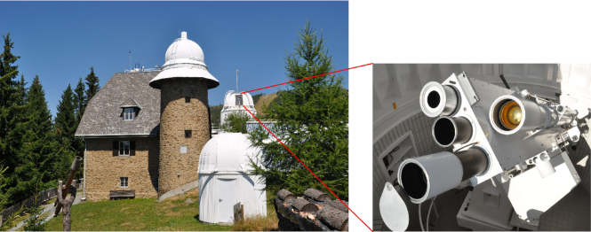
Figure 3.: Kanzelhöhe Observatory (left) and its solar patrol telescope consisting of four refractors observing the Sun in H$\alpha$, Ca ii K and white-light (right).telescope˙fig

3 Image recognition algorithm

algorithm

The developed image recognition algorithms make use of the main characteristics of the features in single H$\alpha$ images as well as in images sequences. Solar flares are characterized by a distinct brightness increase of localized areas on the Sun. They reach their maximum extent and maximum intensity typically within some minutes up to some tens of minutes, followed by a gradual decay of the intensity due to the subsequent cooling of the solar plasma. Flares are categorized in importance classes based on their total area and their brightness enhancement with regard to the quiet Sun level.

The image recognition algorithm consists of four main building blocks. The preprocessing handles the different intensity distributions, large-scale inhomogeneities and noise. The feature extraction step defines the characteristic attributes of the features to be detected, and how to model them. In the multi-label segmentation step, the model is applied to “new”, i.e. previously unseen, images in almost real-time. In the postprocessing, every identified object is assigned and tracked via a unique ID, and the characteristic flare parameters are derived (location, area, start/peak time, etc.) In the following we give a basic description of these methods; further details can be found in Riegler et al. (2013) and Riegler (2013).

3.1 Preprocessing

algo_pre

The preprocessing has two goals, namely image normalization and feature enhancement. Across different H$\alpha$ image sequences, the intensity distributions of the images are shifted and dilated. These differences in the distributions arise due to different solar activity levels (e.g. many/few sunspots), seeing conditions, exposure time, etc. As the feature extraction strongly relies on value of the image intensities, we normalize the image intensities by a zero-mean and whitening transformation:

$$\mu =\frac{1}{|\Omega|}\sum_{x\in\Omega}f(x)$$ (1)

$$\sigma =\sqrt{\frac{1}{|\Omega|-1}\sum_{x\in\Omega}\left(f(x)-\mu\right)^{2}}$$ (2)

$$f_{n}(x) =\frac{f(x)-\mu}{\sigma}$$ (3)

where $\Omega\subset\mathbb{R}^{2}$ is the image domain, $\mu$ the sample mean and $\sigma$ the standard deviation of the input image $f$, respectively. The normalized image $f_{n}$ is given by a point-wise subtraction and division by the mean and standard deviation.

As a second step in the preprocessing, additive noise and large-scale intensity variations, caused by the center-to-limb variation and clouds, are removed by applying a structural bandpass filter. At the core of this particular filtering method is the total variation with $\ell_{1}$ fitting term (TV-$\ell_{1}$) model (Chan and Esedoglu, 2005; Aujol et al., 2006), which is a signal and image denoising method based on minimizing a convex optimization problem given by

$$\min_{u}\|\nabla u\|_{2,1}+\lambda\|f-u\|_{1}$$ (4)

where $f$ is the noisy observation of the image and $u$ is the minimizer of the optimization problem. The first term, the total variation norm, regularizes the geometry of the solution and the second term, the $\ell_{1}$ norm, ensures that the solution is close to the original image $f$. Finally, $\lambda$ is a free parameter that can be used to control the amount of regularization. The main property of the TV-$\ell_{1}$ model is that it is contrast invariant. In other words, structures from the image a removed only in terms of their spatial extent and not in terms of their contrast to the background. To efficiently solve the optimization scheme we use the generic primal dual algorithm proposed in Chambolle and Pock (2011).

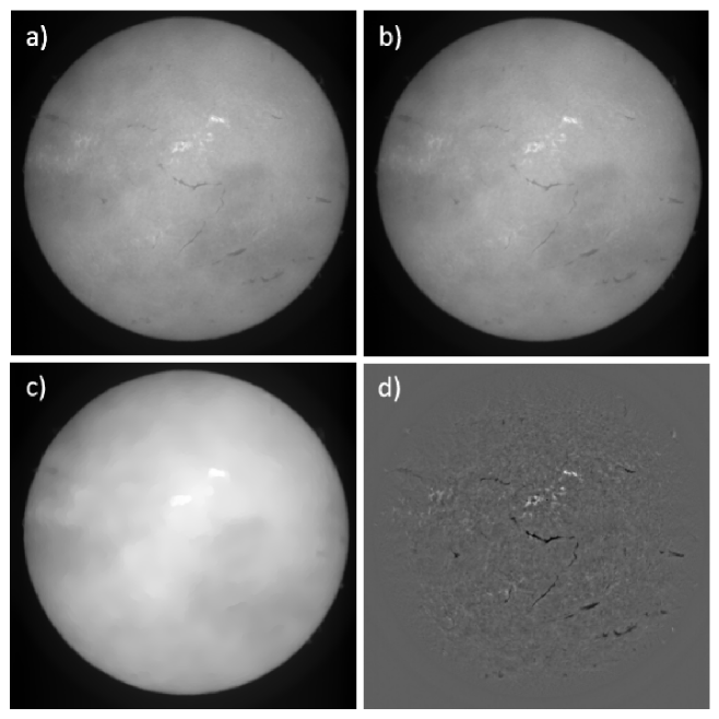
Figure 4.: Structural bandpass filter applied to an H$\alpha$ image with clouds. a) Original image $f$, b) denoised image $v_{1}$, c) large-scale variations $v_{2}$, d) resulting image $u$ of the structural bandpass filter.bandpass˙fig

It was shown in Chan and Esedoglu (2005) that by solving the TV-$\ell_{1}$ for a certain parameter $\lambda$, all structures having a minimal width of $\lambda^{-1}$ are removed in the regularized image $u$. We utilize this fact in our structural bandpass filter by first removing small-scale noise from the image using a larger $\lambda_{1}$, which results in image $v_{1}$. In the next step, we remove larger structures by again regularizing the image $v_{1}$ using a smaller $\lambda_{2}<\lambda_{1}$ such that the resulting image $v_{s}$ contains only unwanted large scale structures such as brightness variations, clouds, etc. The final result of the structural bandpass filter is then given by subtracting image $v_{2}$ from image $v_{1}$.Figure bandpass_fig illustrates the different steps of the structural bandpass applied to a sample KSO H$\alpha$ filtergram with clouds.

3.2 Feature extraction

algo_feat

In the feature extraction step, two main problems have to be addressed. a) What are the characteristic attributes of flares and filaments, i.e. what discriminates them from other solar regions? b) How can we efficiently model these attributes?

To solve the first problem we assign to each pixel a feature vector. The most intuitive feature choice is the pixel intensity of the preprocessed images. We utilize the fact that filaments appear darker than the background of the H$\alpha$ images, and that sunspots are even darker than filaments and have also different typical geometries compared to filaments (round versus elongated objects). Flares are defined as objects with distinctly higher intensities than the background. It may also be useful to use the intensities of the pixels within a small local neighborhood. Further, the contrast decreases from the center towards the limb. To incorporate this effect, the distance from the solar disk center to the pixel location has proven to be useful.

Based on the extracted feature vectors we utilize a Gaussian mixture model to assign each pixel of an H$\alpha$ image a class probability. For the classes we use the features “flare”, “filament” and “sunspot”. The remaining part of the image is summarized in the class “background”.

Figure histogram_fig illustrates the class probabilities in a histogram. The data that we use for the feature extraction and the learning of the model are derived from labeled H$\alpha$ images, where an expert annotated a set of KSO H$\alpha$ images by assigning the pixels to the different classes. As one can see from the figure, the probability distributions of the four classes are not distinctly separated. The overlaps between the classes sunspot–filament and background–flare are no severe problem, because most of the probability mass is well separable. In contrast, the probability distribution overlap between the classes filament–background does cause segmentation problems in the application. Additional methods that can be used to arrive at a better distinction of filaments against the background are described in Riegler (2013).

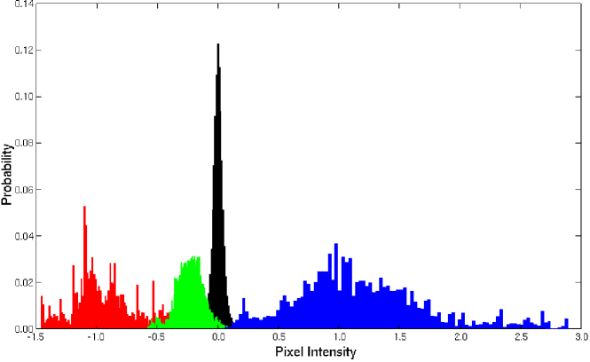
Figure 5.: Intensity distribution of the classes sunspot (red), filament (green), background (black) and flare (red). The training examples are derived from preprocessed H$\alpha$ images that were annotated by an expert. histogram˙fig

3.3 Multi-label segmentation

algo_multi

In principle, each pixel could be assigned to the class with the highest probability, however, this would lead to a very noisy segmentation. In order to regularize the final segmentation, we adopt a total variation based multi-label image segmentation model (Chambolle and Pock, 2011):

$$\min_{\{u_{l}\}_{l=1}^{N}}\sum_{l=1}^{N}\int_{\Omega}\mathrm{d}|\nabla u_{l}|+\sum_{l=1}^{N}\int_{\Omega}u_{l}q_{l}\;\mathrm{d}x$$ (5)

$$\text{s.t.}\quad u_{l}(x)\geq 0,\quad\sum_{l=1}^{N}u_{l}(x)=1,$$ (6)

where the functions $u_{l}$ and $q_{l}$, $l=1...N$ are the binary class assignment functions and class-dependent weighting function, respectively. In the simplest case the negative logarithm of the class probabilities can be used, but we apply an additional temporal smoothing by computing an exponential weighted moving average over the probabilities.

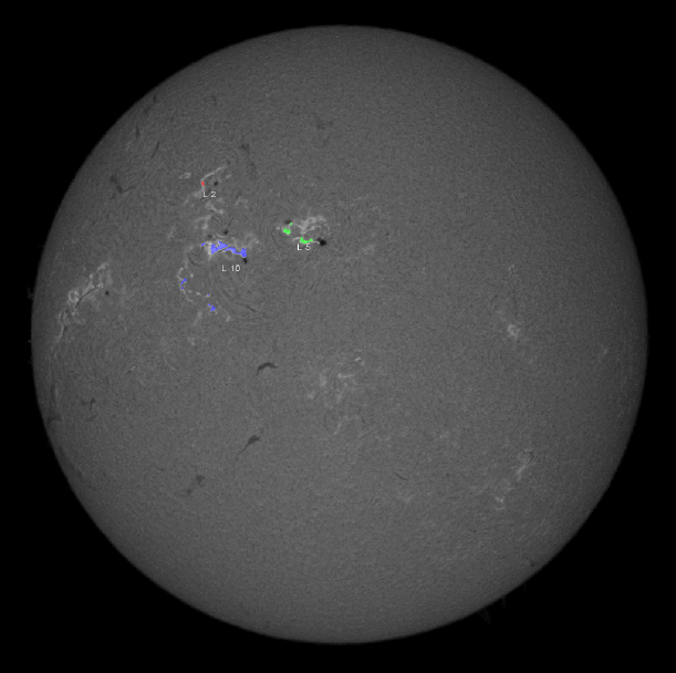
Figure 6.: Sample KSO H$\alpha$ image from May 10, 2014, in which three different flares are simultaneously present on the solar disk. The detected flare areas are indicated in different colors. Each flare is registered and tracked in time, i.e. from image to image by a unique ID. flares˙fulldisk˙fig

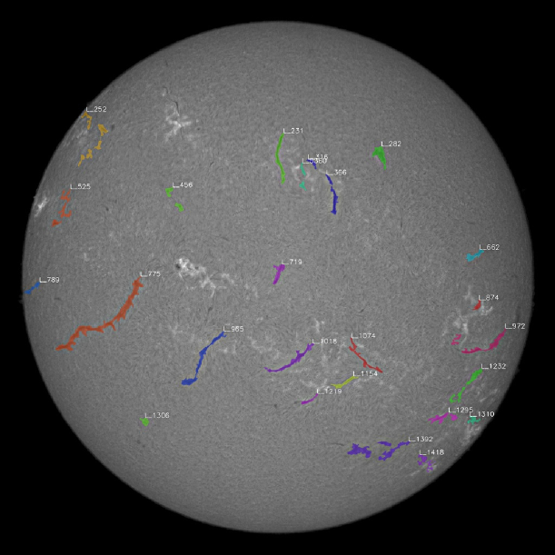
Figure 7.: Sample KSO H$\alpha$ image from March 31, 2014 together with the filament detections. Each filament is assigned and tracked by its unique ID (annotated at each filament). filament˙fig

3.4 Postprocessing

algo_post

The final step of the method is the postprocessing that has two main goals. The first one is the identification of each detected flare (and filament) with a unique ID, which should remain the same over the image sequence for the very same object. The second goal is the derivation of characteristic properties from the identified objects to categorize them.

3.4.1 Identification and tracking

The identification task is solved by means of a connected-component labeling problem (Rosenfeld and Pfaltz, 1966). For the tracking of the objects in the H$\alpha$ image sequence, we apply a simple propagation technique. From the segmentation we obtain the four binary images $u_{l}$ for the four classes. The next step is to identify 8-connected pixels that form a group and are separated through zeros from other groups, and to assign an ID to them. The problem can be efficiently solved with a two-pass algorithm as presented for example in Haralock and Shapiro (1991). In a first pass, temporary labels are assigned and the label equivalences are stored in a union-find data structure. Then a label equivalence is detected, whenever two temporary labels are neighbors. In the second pass, the temporary labels are replaced by the actual labels that are given by the root of the equivalence class. The union-find data structure is a collection of disjoint sets and has two important functions. The union function combines two sets, and the find function returns the set that contains a given number. The data structure can be efficiently implemented with trees.

The connected component labeling ensures that every flare (and filament) has a unique ID per image. To guarantee that the ID remains the same through the image sequence, we propagate the ID of previous images. Assume that $I_{t}(x)$ is the current component labeled segmentation and $\{I_{t-k}(x)\}_{k=1}^{n}$ the set of $n$ previous component labeled segmentation results. Then we change the ID of a current component $I_{t}$ to the ID $j$, where $j$ is given by the components of the previous images that have the most overlap with the component $I_{t}$. This can be implemented in a pixel-wise fashion and a simple map data structure. For a given component of the current image and ID $I_{t}$ we iterate all overlapping pixels $x$ of the set $\{I_{t-k}(x)\}_{k=1}^{n}$. If $I_{t-k}(x)\neq 0$, we increment the counter for the ID $I_{t-k}(x)$ in the map. Finally, we assign the ID with the highest counter. Since flares often consist of two or more ribbons, flare detections that are located within a certain distance (set to 150 arcsec) are grouped to one ID. Figure flares_fulldisk_fig shows a sample H$\alpha$ image with the flare detections and the assigned flare IDs. A sample H$\alpha$ image with the filament detections is shown in Figure filament_fig.

4 Implementation at the KSO H$\alpha$ observing system

data_proc

To optimize the process and speed of the real-time data provision and flare detection, different computers are involved that run in parallel, each one performing a specific set of tasks:

• camera computer: image acquisition;

• workstation 1: quality check, data processing and online data provision;

• workstation 2: image recognition, flare detection and alerting.

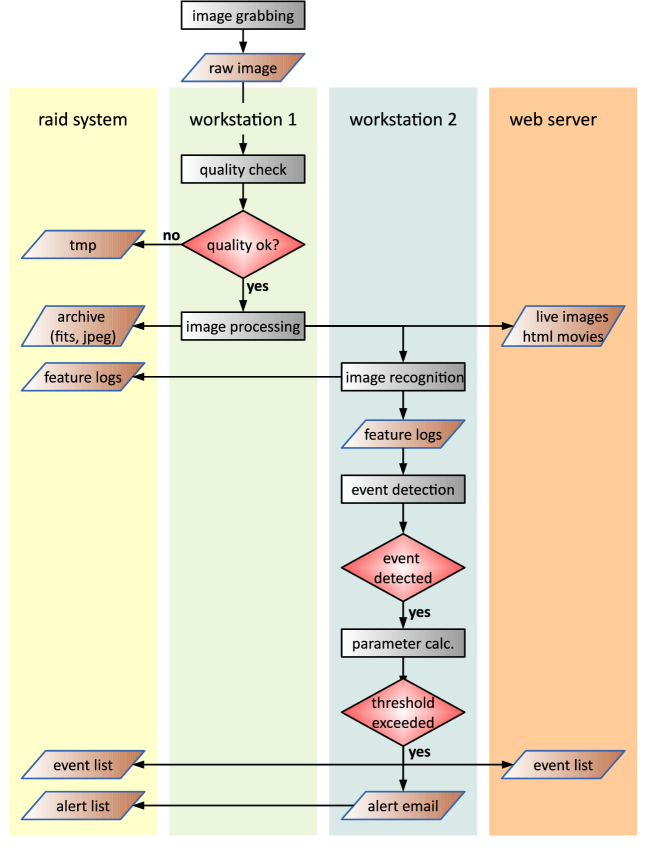
Figure 8.: Flow diagram showing the main steps of the data processing pipeline at the KSO H$\alpha$ observing system. The overall process of data acquisition, quality check, processing, image recognition, event detection and alerting involves four different machines (camera PC, raid system, workstation 1 and 2) and a web server where the results are published. pipeline˙fig

Figure pipeline_fig shows a flow diagram of the tasks that are performed on each incoming H$\alpha$ image, where the columns refer to different machines responsible for certain tasks. Each H$\alpha$ image is grabbed by the camera computer and sent to workstation 1, where the image is checked for its quality. If the quality criterion is passed, the image is processed and published on the web server. In parallel, the processed image is also transferred to workstation 2, on which the image recognition algorithm is performed. If an event is detected, its characteristic parameters are calculated. In case that the event exceeds a certain threshold (i.e. flare area/importance class), a flare alert is published online at ESA’s SSA SWE portal and an alert email is sent out. In the following we give a detailed description of the different analysis steps.

4.1 Image acquisition, processing and online provision

acquisition

Image grabbing

The image acquisition is done in a fully automated mode, which includes automatic exposure control and the use of the frame selection technique (Shine et al., 1995). The CCD camera is controlled via a simple user interface; in standard patrol mode no user interaction throughout the observation day is needed.

Quality check

All H$\alpha$ images grabbed are checked for their quality. Clouds and bad seeing conditions result in low contrast and unsharp images, which may cause difficulties for the image recognition. Since the quality test has to be performed on each image, a simple algorithm was implemented. The image quality is measured by three conditions that have to be fulfilled:

• The solar disk appears as a sphere with high accurateness: points on the solar limb are detected by a Sobel edge enhancement filter. A circle is fitted through the detected limb points and the relative error of the radius is computed.

• The large-scale intensity distribution is uniform: the solar image is rebinned to a 2 x 2 pixels image, and the relative brightness differences of these 4 pixels define a measure of the intensity distribution.

• The image is sharp: the correlation between the raw image and a smoothed version of the image is computed. If the raw image is already unsharp, it shows a high correlation with the smoothed image.

Based on these criteria, the images are classified in three quality groups: good, fair and bad. Only images of quality “good” are sent to the image recognition pipeline and the online data provision. Images classified as “fair” or “bad” are moved to a temporary archive and are not considered in the further analysis. However, we note that images of quality “fair” may still be acceptable and useful for visual inspection (e.g. for visual flare detection).

Image processing

For all images that remain in the pipeline, decisive parameters like the disk center, the solar radius, maximum and mean brightnesses, etc. are derived. Together with additional information such as the acquisition time, instrument details, solar ephemeris for the recording time, etc., the images are stored as FITS file (Pence et al., 2010). These images are on the one hand stored in the KSO data archive, on the other hand they are fed into the subsequent pipeline of real-time data provision and image recognition.

Provision of real-time images and movies on the SSA SWE portal

Each minute an image is selected for the real-time H$\alpha$ display at ESA’s SSA SWE portal (http://swe.ssa.esa.int/web/guest/kso-federated; a snapshot is shown in Figure portal_fig). The size of the image is reduced to 1024$\times$1024 pixels and stored in jpeg format for fast and easy display. The image is overlaid with a solar coordinate grid and annotated with a header containing time information. For later validation, with each image a log file is updated that keeps track of the image acquisition time and the time when the image was provided online. Every five minutes an html-movie script that animates the latest hour of H$\alpha$ images is generated and displayed at the SWE portal.

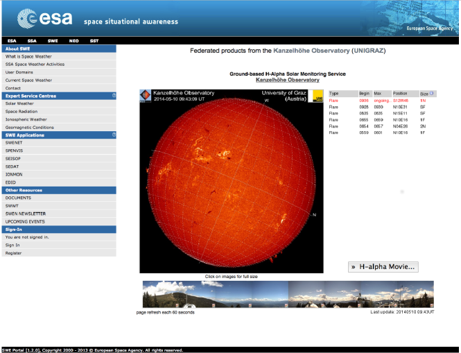
Figure 9.: Screenshot of the ESA SSA SWE H$\alpha$ subportal (http://swe.esa.int/web/guest/kso-federated). The subportal shows the real-time H$\alpha$ image (middle), a list of the detected events of that day (right) and a 360 deg view around the observatory (bottom) for checking the observating conditions, and is updated every minute. portal˙fig

4.2 Image recognition, flare characterisation and alerting

Image recognition

Most of the iterative algorithms of the image recognition (cf. Sect. algorithm) are computationally intensive. However, they can be easily parallelized. Thus, it is possible to utilize the computational power of modern graphic processing units (GPU). The image recognition algorithm has been implemented in the programming language C++ and installed on a dedicated machine with a high-performance GPU. The system benefits from the large number of processing units which are used for the highly parallelized computations. In its present form, the algorithm needs about 10 s to process the flare and filament recognition on one $2048\times 2048$ pixels image, which allows event detection in near real-time. The results of the image recognition algorithm are stored in feature log files containing tables of flares and filaments that have been detected. These feature log files are updated at each time step, i.e. with each new image that enters the pipeline, so that the evolution of the detected features can be computed.

Event detection and parameter calculation

After the detection of a flare by the image recognition system, its characteristic properties and parameters are derived. For flares, these include the heliographic position, the flare area (which defines the importance class), the brightness class, and the flare start and peak times. These quantities need not only the information of a single H$\alpha$ image but also the information stored in the image recognition log files for the previous time steps. Handling of simultaneous flares is easily possible as each flare is identified via a unique ID that is propagated from image to image. In Figure flare_20140510_fig we show a sequence of H$\alpha$ images that were recorded during a 2B class flare that occurred on May 10, 2014 (top panels) together with the segmented flare regions (bottom panels).

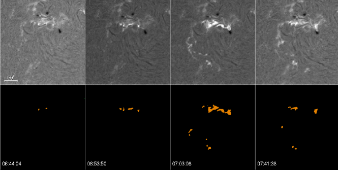
Figure 10.: Top: Sequence of H$\alpha$ images showing the evolution of a 2B flare that occurred on May 10, 2014. Bottom: segmented flare areas. flare˙20140510˙fig

The flare area is calculated by the number of segmented pixels with the same ID. These are subsequently converted by the pixel-to-arcsec scale of that day to derive the area in millionths of the solar hemisphere, so-called “micro-hemisphere”. The conversion procedure includes the information of the flare position to correct the effect of foreshortening toward the solar limb. The determined area is then directly converted to the flare importance class (subflares, 1, 2, 3, 4) according to the official flare importance definitions (cf. Table flare_def). For the categorization into the flare brightness classes (Brilliant-Normal-Faint: B-N-F), the intensity values relative to the background are used. To this aim, we compute the mean, standard deviation, maximum and minimum of the pixel intensities within the segmented regions. For each detected feature, we apply a normalisation by the difference between the maximum brightness and the mean brightness of the feature.

Table 1.: H$\alpha$ flare importance classes.flare˙def

H$\alpha$ importance	Flare area
	(micro-hemisphere)
S[ubflares]	$<$ 100
1	100 – 250
2	250 – 600
3	600 – 1200
4	$>$ 1200

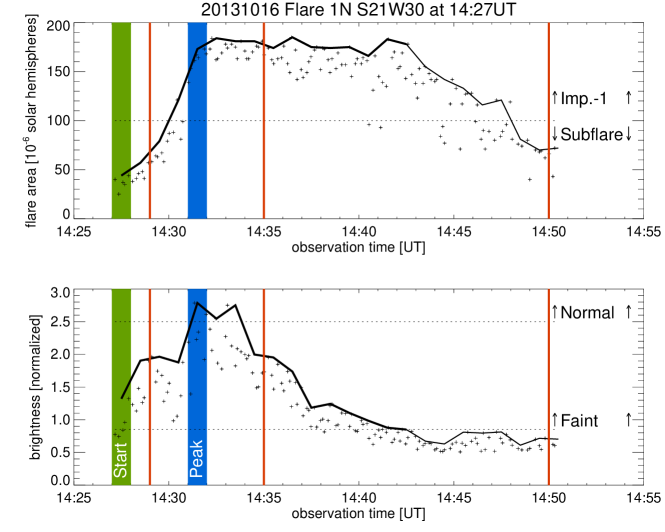
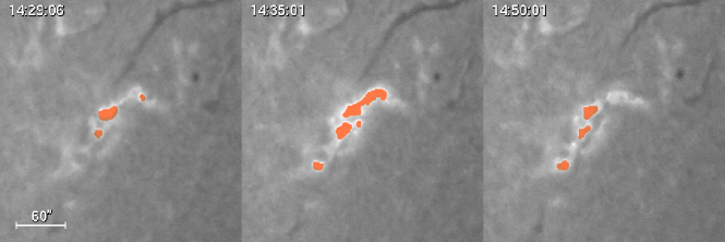
Figure 11.: Illustration of the flare parameter calculation for the 1N flare of October 16, 2013. Top: Evolution of the flare area. Middle: Evolution of the flare brightness. The crosses show the data points, the solid line shows the maximum values for each minute. The thick solid line represents times where the intensity is above the faint flare level. The determined start (14:27 UT) and peak (14:31 UT) times are indicated by the green and blue bar, respectively. Note that the maximum brightness and the maximum area do not necessarily occur at the same time. Bottom: Snapshots of the flare at three different times (indicated by orange vertical lines on the top panels) together with the flare detections. area˙bright˙fig

To characterize a flare, the evolution of the brightness and the area in each H$\alpha$ image of the sequence has to be analyzed. For illustration, we show in Figure area_bright_fig the evolution of the area and brightness of a sample 1N flare that occured on October 16, 2013. The flare classification is based on the following definitions:

1. The flare start is defined as the time when the brightness enhancement is above the faint flare level for 3 consecutive images.

2. The peak time of the flare is defined as the time where the maximum flare brightness is reached.

3. The flare position is defined by the location of the brightest flare pixel at the time of the flare peak.

4. The importance class of the flare is defined via the maximum area of the flare, and is updated when the area exceeds the level of a higher importance class.

5. The flare end is defined as the time when the brightness has decreased below the faint level for 10 consecutive images or when there is a data gap of more than 20 minutes.

6. Handling of data gaps: In case of data gaps $<$20 min, the flare is considered to be in an evolving state if the flare brightness after the data gap is higher than before the gap. Data gaps of $>$20 minutes define the end of the flare.

Flare alerts

If a flare is detected that exceeds a certain threshold, i.e. importance class, then a flare alert is published on the ESA SSA SWE portal and an alert email is sent out to registered users. Originally, it was intended to restrict the flare alerting to events of H$\alpha$ importance class 1 and higher. However, due to the weak activity cycle 24, we lowered the threshold to subflares exceeding a size of 50 micro-hemispheres, in order to obtain a sufficient statistics for the evaluation.

The event list on the ESA SSA SWE portal is updated every time a flare is detected, when more information on flare becomes available during its evolution (e.g., the peak time) or when a flare that is already listed increases in its importance class. The flares are sorted in decreasing start time, so that the most recent event appears in the first line of the table. As long as the flare brightness increases, no peak time is listed but the event is annotated to be “ongoing” and marked in red color in the event list in the H$\alpha$ subportal (cf. Fig. portal_fig). When the flare brightness has decreased for $>$2 min, the peak time is derived and provided in the event table. A list of all detected events is stored in the local raid system for later evaluation.

In addition, flare alert emails are sent to a predefined list of users. They are issued when one of the following criteria is fulfilled: i) The flare detected is of importance class 1 or higher or a subflare with an area exceeding 50 micro-hemispheres, or ii) an ongoing flare reaches a higher importance class (e.g., a flare of importance 1 evolves further to a flare of importance 2).

5 Results

The system of near real-time H$\alpha$ data provision, automatic flare detection and alerting went online on June 26, 2013. In the following we present the results from evaluating the system for a period of five months from June 26 to November 30, 2013, in which it was run with the same set of parameters and definitions.

5.1 Real-time data provision

To validate the online data provision, we evaluated the number of H$\alpha$ images that were recorded by the KSO observing programme and the number of H$\alpha$ images that were provided online in almost real-time at the ESA SWE service portal. For this purpose, log files recorded for each image both the observation time and the time when the image was put online to the SWE service portal.

During the evaluation period, we had in total $563$ hours of solar observations at KSO. In total, 395 129 H$\alpha$ images were recorded. $281\,806$ images (71.3%) were rated as “good”, 20 922 (5.3%) as “fair”, and 92 401 (23.4%) as “bad”. 33 765 H$\alpha$ images (one per minute) out of the “good” sample were provided online at the SWE service portal, whereas 14 were erroneously skipped due to internal data stream errors. This means that in $99.96$% of the observation time, one image per minute was provided online at the SWE portal. The mean time lag between the recording of an image and its online provision was $3.6\pm 0.9$ seconds.

5.2 Real-time flare detection and classification

For the evaluation of the automated detection and alerting of H$\alpha$ flares, we considered all flares that exceeded an area of $50$ micro-hemispheres and that occurred within 60^∘ from solar disk center during the KSO observing times. As discussed in Sect. acquisition, only images of quality “good” are fed into the automatic flare detection pipeline. For the automatic detection of a flare, we demand that it is observed in at least three H$\alpha$ images. Periods of $>$20 min containing no images of quality “good” are defined as data gaps.

The data that are needed for the evaluation of the flare detection, classification and alerting are derived from the log files that are created and updated during the observations (cf. Fig. pipeline_fig). The relevant parameters that are derived and evaluated are:

• Flares: heliographic position, start time, peak time, area, importance class, brightness class;

• Alerts: time of issue.

For the evaluation, we compare the results obtained by the automated image recognition system developed, called Surya, against the official flare reports provided by the National Geophysical Data Center (NGDC) of the National Oceanic and Atmospheric Administration (NOAA) and by Kanzelhöhe Observatory. Both are obtained by visual inspection of the data by experienced observers.

The Space Weather Prediction Center (SWPC) of the U.S. Department of Commerce, NOAA, is one of the national centers for environmental protection and provides official lists of solar events, online available at http://www.swpc.noaa.gov/ftpmenu/indices/events.html. The information on the flare events is collected from different observing stations from all over the world. Kanzelhöhe Observatory sends monthly flare reports to different institutions, including NGDC/ NOAA and the World Data Center (WDC) for Solar Activity (Observatoire de Meudon). The visual KSO flare reports (KSOv) are online available at http://cesar.kso.ac.at/flare˙data/kh˙flares_query.php. We actually expect that the results of the automatic detections are on average closer to the visual KSO flare reports than the NOAA reports, as they are based on the data from the same observatory. However, it is also important to compare the outcome against the NOAA reports, as they provide an independent set of flare reports.

Table tab:flares1 in the Appendix lists all flare events (area $\geq 50$ micro-hemispheres; located within $60^{\circ}$ from disk center) which were detected in quasi real-time by the automated algorithm during the evaluation period. In total, $87$ flares were detected by Surya; $69$ were classified as subflares and $18$ as flares of importance 1. This list includes $3$ false detections (marked in red color in the table), i.e. flares that were detected by Surya but have no corresponding event reported by NOAA or KSOv. In addition, the list in Table tab:flares1 includes 7 flares where Surya reported one flare but NOAA and KSOv reported two separate events, as well as 2 NOAA (4 KSOv) flares, where Surya has split up one flare into two or more events.

To evaluate the detection ability of Surya, we checked also all NOAA and KSOv flares reported during the KSO observation times (located within 60^∘ from disk center) that were not detected by Surya. These are in total $60$ flares (57 SF, 2 SN and one 1N flare). There are basically two different reasons why these events were not detected by Surya:

1. Data gaps: Less than 3 images of quality “good” were available during the event, and thus the automatic detection algorithm was not run. 47 flares fall into this category. We note that single images as well as images of lower quality may still be sufficient to identify a flare by visual inspection (though with large uncertainties in the derived flare parameters). Indeed, for 19 out of these events visual flare reports from KSOv are available (18 subflares, and one flare of importance 1).

2. NOAA reports a flare which is not listed by KSOv and where – even after careful visual re-inspection of the KSO H$\alpha$ image sequences – we cannot confirm the appearance of a flare. This applies to $13$ events, all of them subflares.

Given the reasons above, these events are not expected to be detected by our automatic image recognition system. This means that Surya basically detected all flares listed by the NOAA and KSOv flare reports, when there were sufficient data available (i.e. at least three images during an event).

The next question we have to address is how accurate are the flare parameters calculated by the automatic system. The accuracy of the peak flare area determined by Surya cannot be evaluated, since the flare reports do not provide areas. However, the flare area is an intrinsic property which determines the importance classification of a flare (cf. Table flare_def). For the importance classifications we find that there are 7 cases, in which the importance classes reported by NOAA and KSOv do not conincide. Thus we excluded those events from the evaluation of the importance classes as there is no unique reference value available. For the remaining set of flares, we find that in 86% the automatically determined flare importance class coincides with the class given by NOAA and KSOv. The incorrectly classified events include 5 flares where Surya obtained a different importance class than reported by NOAA and KSOv, and 6 cases where Surya has split up flares in 2 or more events. For the brightness classification, there are 15 events where the NOAA and KSOv reports do not coincide. For the remaining set, we find that in 85% Surya determined the correct brightness class (cf. Table tab:flares1).

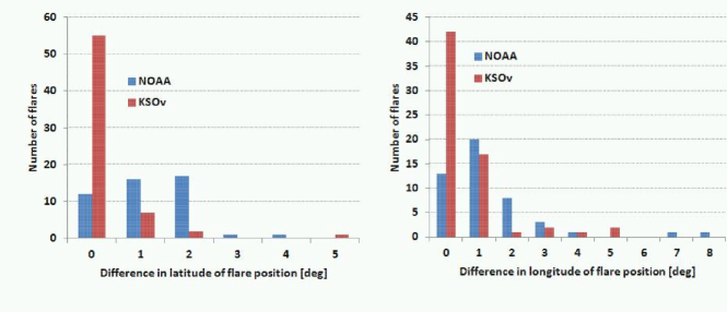
Figure 12.: Distribution of the absolute differences of the flare’s heliographic latitude (left) and longitude (right) between the automatic detection by Surya and the NOAA (blue) and KSOv (red) reports.fig:diffLon

Figure fig:diffLon shows the absolute differences of the heliographic latitude and longitude of the flare center as obtained by the automatic algorithm against the values reported by NOAA and KSOv. The mean of the absolute difference for the latitude is $1.21^{\circ}$ ($0.25^{\circ}$) with respect to the NOAA (KSOv) flare reports, and $1.36^{\circ}$ ($0.60^{\circ}$) for the longitude.

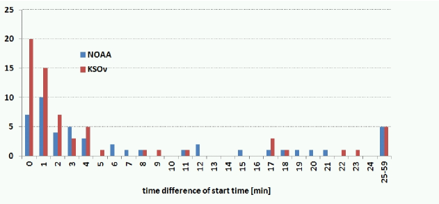
Figure 13.: Distribution of the absolute differences between start times of the flares detected by Surya and reported by NOAA (blue) and KSOv (red).fig:diffStart

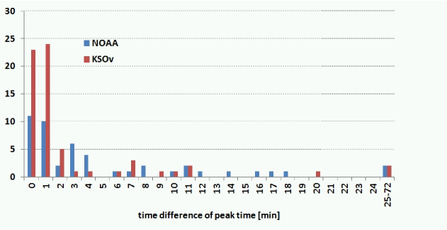
Figure 14.: Distribution of the absolute differences between peak times of the flares detected by Surya and reported by NOAA (blue) and KSOv (red).fig:diffPeak

Figures fig:diffStart and fig:diffPeak show the distributions of the absolute differences of the flare start times and peak times, respectively, derived by Surya in comparison to NOAA and to KSOv. For the start and the peak times, the median time difference is $3$ min (1 min) with respect to NOAA (KSO). For $62$% ($78$%) of the flares detected, the derived flare start times lie within $\pm 5$ min with respect to the NOAA (KSOv) reports, and for $70$% ($83$%) the flare peak times lie within $\pm 5$ min with respect to NOAA (KSOv).

5.3 Real-time flare alerts

When a flare reaches a certain threshold, an alert email is automatically generated and sent to a predefined list of users. The expected number of alerts is actually higher than the number of detected Surya flares listed in Table tab:flares1, since alerts are not only sent for the detection of an event but also in the case where the flare evolves to a higher importance class. This means that for a flare of importance 1, we have two alerts when the full flare evolution was covered: one when it reaches the level of a subflare of area $\geq$50 micro-hemisphere, and another one when it reaches an area of 100 micro-hemispheres, i.e. the threshold for an importance 1 flare. In total, we had 14 cases (14%) where erroneously no flare alert emails were issued. These include the 4 flares on July 21, 2013, the 5 flares on Oct 11, 2013 and the first 2 flares on Oct 15, 2013, where we had an error in the automatic email script. In addition, no alert was sent for 3 flares that reached exactly the threshold area of 50 micro-hemispheres (Aug 15, 2013, 12:03 and and 12:49; Aug 30, 2013, 06:14). The total number of false alerts was six. Three of the false alerts are related to the false flare detections (indicated in red in Table tab:flares1). The other three false alerts were double alerts, i.e. two identical emails had been sent for one flare.

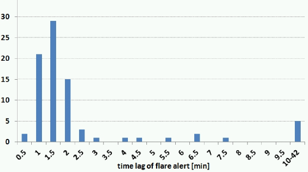
Figure 15.: Distribution of the time differences between the start of the flare and the issue of the alert.fig:diffAlert

We also evaluated the time between the occurrence of the flare and the issue of the alert email. In this respect, occurrence means the time when the flare reaches the threshold area, i.e. an area of $50$ micro-hemispheres for a subflare alert, or an area of $100$ micro-hemispheres for an importance $1$ alert, etc. Figure fig:diffAlert shows the distribution of the time difference between the occurrence of the flare and the issue of the alert email, giving a median of $1.5$ min. In total, $89$% of the (true) alerts were issued within $5$ minutes. However, we note that there are five cases where the delay is larger than $10$ min. These are mostly related to data gaps in the H$\alpha$ image sequences. The detection of a flare demands that a flare is detected in at least three observations. However, if there is a longer data gap, say, between the second and the third image of a sequence, then the alert (which is issued after the flare detection in the third image) may occur substantially delayed with respect to the start of the flare (defined by the time of the first image in this sequence).

6 Discussion and Conclusions

The real-time H$\alpha$ data provision worked perfectly fine, with a percentage of $99.96$% provisions online at the ESA SWE portal within less than 4 s of the observations. The automatic flare detections basically worked in all cases within the given criteria, i.e. within the demand that for a positive detection we need at least three H$\alpha$ images of quality “good” during the event. In our 5-month evaluation period, about 70% of all the H$\alpha$ images observed at KSO (with a regular cadence of 6 s) were classified as “good”. We note that for visual classifications by an experienced observer also fewer images or images of lower quality may suffice but result in flare parameters with large uncertainties. This is reflected in the number of 87 flares that were detected by the automatic system, whereas the KSO visual reports included 19 additional events (18 SF, one 1N).

The automatically determined flare importance and brightness classifications were correct in about 85% of the events. The misclassification of 15% is comparable to the $\sim$7% (17%) inconsistencies between the NOAA and KSOv flare reports for the importance (brightness) class. These differences in the official reports are related to different instruments, seeing conditions and observers that derived the parameters. The mean of the calculated heliograpic longitude and latitude of the flare center was consistent with the official flare reports within $\sim$1^∘. The median of the absolute differences between the flare start and flare peak times of the automatic detections in comparison to the NOAA (KSOv) reports were 3 min (1 min). In $\sim$90% of the flare alert emails that were sent, the alert was issued within 5 min of the flare start. However, 15% of the expected alerts had been not sent. The number of false flare detections and alerts was less than 6% compared to the total number of (true) alerts issued.

We note that our event set consisted mostly of subflares (69) and importance 1 flares (18). There was one event reported as $2$N by NOAA and KSOv (October 10, 2013; cf. Table tab:flares1), which was misclassified as $1$F by our automatic algorithm. Re-inspection of the processing of this event showed that the area had been correctly calculated (i.e. exceeded the threshold to an importance 2 flare), but due to a large data gap during the observing sequence, the algorithm erroneously applied a wrong time (during the flare decay phase) for the calculation of the importance class.

We conclude that the automatic flare detection implemented at KSO and provided online at ESA’s SSA SWE portal provides reliable and near real-time detection, classification and alerting of solar H$\alpha$ flares. The information on the flare timing, strength and heliographic position (which relates to the magnetic connectivity to Earth) that is derived in near real-time could, e.g., be connected to SEP models. We note that the largest challenges of the algorithm are actually the handling of data gaps, which are the largest source of misclassification of the flare class and the split-up of one flare into more than one. Further systematic evaluation of the system at times of higher solar activity and more frequent occurrence of larger flares will be valuable in order to test its ability for the automatic detection of the most severe space-weather effective events.

Table tab:flares1 lists all flares detected by Surya with an area $\geq$ $50$ micro-hemispheres and located within 60^∘ of the solar disk during the period June 26 to November 30, 2013 together with the corresponding information from the NOAA and KSOv flare reports. Column $1$ gives the observation date, columns $2-4$ list the start time of the flare (from Surya, NOAA, KSOv), columns $5-7$ the peak time, columns $8-10$ the heliographic position, columns $11-13$ the flare type and column $14$ the flare area as determined by Surya. False flare detections by Surya are marked in red color.

Table 2.: Automatically detected flares in the period June 26 to November 30, 2013. Flares marked in red color are false detections.

Start time

Peak time

Position

Type

Area

Surya

NOAA

KSOv

Surya

NOAA

KSOv

Surya

NOAA

KSOv

Surya

NOAA

KSOv

Surya

27/06

09:38

B09:38

09:38

09:41

U09:42

09:41

S16E23

S16E25

S16E23

SF

SF

SF

60

30/06

09:11

09:14

09:33

09:16

S15W20

S16W19

SF

SF

74

04/07

09:21

09:22

S11E45

SF

50

05/07

04:26

B05:25

05:01

05:16

U05:34

05:16

S08E30

S06E38

S08E30

SF

SF

SF

87

06:57

06:58

06:57

06:59

07:03

06:59D

S09E30

S09E33

S09E29

SF

SF

SF

60

09/07

07:38

07:38E

07:40

07:40U

S08W23

S13W18

1F

1F

156

08:32

08:36

S08W24

SF

115

13:27

13:26

13:27

13:31

13:31

13:32

S10W21

S12W21

S10W21

SN

1N

SN

82

10/07

06:20

06:21

06:20U

06:32

06:43

06:31D

S14W13

S15W13

S14W13

1F

1N

1N

177

07:07

07:08

S13W15

SF

72

16/07

10:11

10:12

10:10

10:20

10:16

10:20

S12E03

S12E04

S12E03

SF

SF

SF

96

21/07

06:41

06:43

06:41

06:44

06:44

06:45

N22W07

N23W07

N22W08

SF

SF

SF

61

08:25

08:25

08:25

08:30

08:41

08:31

S07E30

S06E31

S07E31

1F

1F

1F

151

12:16

12:17

12:17

12:19

12:18

12:18

N22W09

N22W09

N22W09

SN

SF

SN

51

14:13

14:11

14:13

14:14

N23W11

N24W11

SF

SF

65

25/07

06:05

06:05

06:05E

06:08

06:07

06:08

S06W20

S08W22

S06W20

SN

SF

SN

59

28/07

12:07

12:05

12:05

12:23

12:23

12:22

S11W59

S13W60

S11W59

SF

SF

SF

70

06/08

08:03

08:04

08:04

08:04

08:04

08:04

N17W01

N15W01

N17W00

SF

SF

SF

65

08/08

05:33

05:39

05:31E

05:34

05:43

05:45U

S13W10

S14W08

S13W09

SF

SF

SF

54

05:41

05:42

S13W08

SF

60

11/08

07:09

07:51

08:04

07:57

S20E31

S20E31

SF

SF

54

12/08

09:49

09:49

09:49

10:43

09:49

09:53

S21E18

S17E20

S21E19

1N

SF

SF

141

10:23

10:22

10:40

10:37

S17E19

S21E19

SN

1N

15/08

12:03

12:03

12:20

12:20

S06E04

S06E04

SF

SF

50

12:37

12:37

12:44

12:45

S06E01

S06E01

SF

SF

54

12:49

12:49

S06E01

SF

50

tab:flares1

Table 3.: Table tab:flares1 continued.

Start time

Peak time

Position

Type

Area

Surya

NOAA

KSOv

Surya

NOAA

KSOv

Surya

NOAA

KSOv

Surya

NOAA

KSOv

Surya

17/08

10:18

10:11

10:09

10:55

10:18

10:19

S05W28

S08W24

S07W23

SN

SF

SN

61

10:55

10:53

10:56

10:56

S07W25

S05W28

SF

SN

19/08

05:42

05:43

05:48

05:46

N15W16

N15W17

SF

SF

63

21/08

07:13

07:17

07:17

07:18

07:17

07:18

S13W38

S15W36

S13W38

SF

SF

SF

78

07:30

07:29

07:29

07:30

07:42

07:37

N16E57

N14E55

N16E57

SF

SF

SF

98

08:33

B09:06

09:06

09:11

U09:11

09:10

S13W38

S15W37

S13W38

SF

SF

SF

75

09:09

09:09

S14W40

SF

22/08

11:45

B11:49

11:46

11:48

U11:58

11:47

N15E37

N17E38

N14E35

SF

SF

SF

65

23/08

05:18

05:17E

05:19

05:18

N12W53

N12W52

SF

SN

69

30/08

06:14

06:14

N16E44

SF

50

04/09

05:32

05:34

05:32

05:40

05:39

05:40

S16W35

S19W35

S16W35

SB

SF

SB

82

06:39

06:47

S16W36

SF

59

06:56

06:57

07:01

07:23

S16W36

S16W36

SF

SF

72

07:11

07:12

S16W37

SF

77

07:18

07:21

07:20

07:26

S16W37

S16W38

SF

SF

88

07:50

07:51

S16W37

SF

59

07:55

07:59

07:59

08:03

S16W36

S16W36

SF

SF

66

08:02

08:03

S16W36

SF

69

08:21

08:18

08:17

08:42

08:39

08:40

S16W36

S18W37

S16W37

SF

SF

1N

79

10:16

09:59

09:59

10:16

10:18

10:16

S16W37

S18W36

S16W37

SF

SF

SF

66

11:42

B11:45

11:50U

12:30

U11:45

12:19

S16W39

S18W38

S16W39

SF

SF

SF

54

12:08

12:14

S18W38

SF

11/10

12:19

12:19E

12:21

12:20U

S24E40

S24E43

SF

SF

71

14:16

14:34

14:33

14:38

14:46

14:47

S09E13

S09E14

S09E13

1N

SF

SF

130

15:06

15:08

S11E14

SF

91

15:25

15:26

S09E12

SF

90

tab:flares2

Table 4.: Table tab:flares1 continued.

Start time

Peak time

Position

Type

Area

Surya

NOAA

KSOv

Surya

NOAA

KSOv

Surya

NOAA

KSOv

Surya

NOAA

KSOv

Surya

15/10

06:50

06:49

07:02

07:01

S21W14

S22W15

SF

SF

76

08:02

08:14

08:01E

08:39

08:15

08:01E

S21W13

S22W14

S21W13

1N

SF

SF

235

08:33

08:23U

08:39

08:39

S22W13

S21W13

SN

1B

08:57

09:09

09:00

09:14

09:15

09:14

S10W35

S10W36

S10W35

SF

SF

SF

80

16/10

08:51

09:12

09:12

09:20

U09:20

09:20

S09W42

S11W41

S09W42

SF

SF

SF

94

13:55

13:55

13:58

13:58

S09W44

S10W44

SF

SF

72

14:27

14:27

14:26

14:31

14:31

14:32

S21W30

S23W29

S21W30

1N

1N

1B

185

17/10

10:21

10:27

10:26

10:29

10:29

10:29

S09W56

S11W56

S09W56

SF

SN

SN

74

11:15

11:48

11:47

13:15

U12:03

12:04

S09W58

S11W56

S10W54

SF

SF

SF

61

20/10

08:38

08:36

08:36

08:42

08:39

08:41

N22W32

N22W33

N22W32

1N

SF

1N

133

09:39

09:40

09:40

09:57

09:43

09:50

N12E43

N11E40

N12E42

1F

SF

SF

135

10:01

10:22

N09E37

1F

136

11:54

11:58

11:55

12:48

U12:16

12:19

N11E41

N12E39

N11E41

1F

SF

SF

167

12:41

12:42

12:40

12:48

U12:45

12:46

N22W34

N22W35

N22W34

SF

SF

SF

75

22/10

07:35

07:35

07:41

07:42

N09E16

N09E15

SF

SF

73

08:33

08:29U

08:34

08:34U

N06E13

N06E13

SF

SF

85

13:30

13:27

13:27

13:32

13:29

13:31

N05E04

N06E04

N04E04

SF

SF

SN

94

26/10

07:33

07:36

N04W38

SF

90

07:50

07:56

N04W38

SF

58

07:58

07:58

08:04

08:03

S10W22

S10W22

SN

SF

74

08:23

B08:54

08:26

08:56

U08:55

08:55

S11W23

S12W23

S11W23

1B

SF

1B

127

08:47

09:18

09:19

09:21

S09E55

S09E54

1B

1B

139

09:01

09:23

09:25

09:25

N07W48

N07W49

1B

1B

123

09:26

09:32

S11W23

SN

72

10:22

10:27

S07E57

SF

59

10:32

B10:11

10:30

11:00

U11:08

11:10

S06E58

S05E58

S06E58

1N

1N

1N

130

10:54

10:54

11:08

11:08

S11W24

S11W24

SF

SF

57

13:18

13:18

13:18

13:20

13:20

13:20

S11W26

S12W25

S11W26

SF

SF

SF

71

tab:flares3

Table 5.: Table tab:flares1 continued.

Start time

Peak time

Position

Type

Area

Surya

NOAA

KSOv

Surya

NOAA

KSOv

Surya

NOAA

KSOv

Surya

NOAA

KSOv

Surya

27/10

10:18

10:16E

10:19

10:18U

S08E43

S08E43

SF

SF

54

11:00

10:59

11:00

11:01

S08E43

S08E43

SF

SF

69

12:13

12:33

12:30

12:39

12:38

12:39

N08W63

N06W63

N08W63

SF

1F

1F

80

28/10

11:10

11:25

11:28E

11:29

11:36

11:28

S06E27

S06E30

S07E28

SF

SF

SF

51

11:52

11:33

11:50E

11:52

11:49

11:51

S14W43

S16W44

S14W43

1F

2N

2N

122

12:13

11:50E

12:13

11:53

S07E28

S05E31

1F

1N

154

01/11

09:26

B09:51

10:08

09:54

S11E04

S12E06

SB

SF

63

10:05

10:12

S12E03

SF

10:50

10:51

S16E07

SF

61

11:08

11:09

S17E08

SF

51

07/11

10:28

10:28

10:28

10:29

10:29

10:31

N21W36

N21W37

N21W37

SF

SF

SF

67

12:16

12:17

12:17

12:28

12:28

12:28

S13E23

S13E24

S13E23

SN

SF

SN

55

29/11

09:55

10:03

09:55

10:10

10:06

10:10

S06W23

S05W16

S06W23

1F

SF

1F

145

tab:flares4

Acknowledgements

This study was developed within the framework of ESA Space Situational Awareness (SSA) Programme (SWE SN IV-2 activity). The authors thank Alexi Glover and Juha-Pekka Luntama for their support, constructive criticism and confidence in the project.

References

- Ahmed et al. (2013) Ahmed, O.W., Qahwaji, R., Colak, T., Higgins, P.A., Gallagher, P.T., Bloomfield, D.S.: 2013, Solar Flare Prediction Using Advanced Feature Extraction, Machine Learning, and Feature Selection. Sol. Phys. 283, 157 – 175. DOI. ADS.
- Aujol et al. (2006) Aujol, J.-F., Gilboa, G., Chan, T., Osher, S.: 2006, Structure-texture image decomposition—modeling, algorithms, and parameter selection. International Journal of Computer Vision 67(1), 111 – 136.
- Benz (2008) Benz, A.O.: 2008, Flare Observations. Living Reviews in Solar Physics 5, 1. DOI. ADS.
- Bonte et al. (2013) Bonte, K., Berghmans, D., De Groof, A., Steed, K., Poedts, S.: 2013, SoFAST: Automated Flare Detection with the PROBA2/SWAP EUV Imager. Sol. Phys. 286, 185 – 199. DOI. ADS.
- Caballero and Aranda (2013) Caballero, C., Aranda, M.C.: 2013, Automatic Tracking of Active Regions and Detection of Solar Flares in Solar EUV Images. Sol. Phys.. DOI. ADS.
- Chambolle and Pock (2011) Chambolle, A., Pock, T.: 2011, A first-order primal-dual algorithm for convex problems with applications to imaging. Journal of Mathematical Imaging and Vision 40(1), 120 – 145.
- Chan and Esedoglu (2005) Chan, T.F., Esedoglu, S.: 2005, Aspects of total variation regularized l1 function approximation. SIAM Journal on Applied Mathematics 65(5), 1817 – 1837.
- Fletcher et al. (2011) Fletcher, L., Dennis, B.R., Hudson, H.S., Krucker, S., Phillips, K., Veronig, A., Battaglia, M., Bone, L., Caspi, A., Chen, Q., Gallagher, P., Grigis, P.T., Ji, H., Liu, W., Milligan, R.O., Temmer, M.: 2011, An Observational Overview of Solar Flares. Space Sci. Rev. 159, 19 – 106. DOI. ADS.
- Haralock and Shapiro (1991) Haralock, R.M., Shapiro, L.G.: 1991, Computer and robot vision, Addison-Wesley, ???.
- Henney et al. (2011) Henney, C.J., MacKenzie, D., Hill, F., Mills, B., Pietrzak, J.: 2011, Solar Flare Detection With SWIFT and Real-time GONG H-alpha Images. In: AAS/Solar Physics Division Abstracts #42, 2233. ADS.
- Hirtenfellner-Polanec et al. (2011) Hirtenfellner-Polanec, W., Temmer, M., Pötzi, W., Freislich, H., Veronig, A.M., Hanslmeier, A.: 2011, Implementation of a Calcium telescope at Kanzelhöhe Observatory (KSO). Central European Astrophysical Bulletin 35, 205 – 214. ADS.
- Joshi and Pant (2005) Joshi, B., Pant, P.: 2005, Distribution of H flares during solar cycle 23. A&A 431, 359 – 363. DOI. ADS.
- Kirk et al. (2013) Kirk, M.S., Balasubramaniam, K.S., Jackiewicz, J., McNamara, B.J., McAteer, R.T.J.: 2013, An Automated Algorithm to Distinguish and Characterize Solar Flares and Associated Sequential Chromospheric Brightenings. Sol. Phys. 283, 97 – 111. DOI. ADS.
- Otruba and Pötzi (2003) Otruba, W., Pötzi, W.: 2003, The new high-speed H imaging system at Kanzelhöhe Solar Observatory. Hvar Observatory Bulletin 27, 189 – 195. ADS.
- Otruba, Freislich, and Hanslmeier (2008) Otruba, W., Freislich, H., Hanslmeier, A.: 2008, Kanzelhöhe Photosphere Telescope (KPT). Central European Astrophysical Bulletin 32, 1 – 8. ADS.
- Pence et al. (2010) Pence, W.D., Chiappetti, L., Page, C.G., Shaw, R.A., Stobie, E.: 2010, Definition of the Flexible Image Transport System (FITS), version 3.0. A&A 524, A42. DOI. ADS.
- Piazzesi et al. (2012) Piazzesi, R., Berrilli, F., Del Moro, D., Egidi, A.: 2012, Algorithm for real time flare detection . Memorie della Societa Astronomica Italiana Supplementi 19, 109. ADS.
- Pötzi, Hirtenfellner-Polanec, and Temmer (2013) Pötzi, W., Hirtenfellner-Polanec, W., Temmer, M.: 2013, The Kanzelhöhe Online Data Archive. Central European Astrophysical Bulletin 37, 655 – 660. ADS.
- Pötzi et al. (2014) Pötzi, W., Riegler, G., Veronig, A., Pock, T., Möstl, U.: 2014, A system for near real-time detection of filament eruptions at Kanzelhöhe Observatory. In: IAU Symposium, IAU Symposium 300, 519 – 520. DOI. ADS.
- Priest and Forbes (2002) Priest, E.R., Forbes, T.G.: 2002, The magnetic nature of solar flares. A&A Rev. 10, 313 – 377. DOI. ADS.
- Qahwaji, Ahmed, and Colak (2010) Qahwaji, R., Ahmed, O., Colak, T.: 2010, Automated Feature Detection and Solar Flare Prediction Using SDO Data. In: 38th COSPAR Scientific Assembly, COSPAR Meeting 38, 2877. ADS.
- Qu et al. (2003) Qu, M., Shih, F.Y., Jing, J., Wang, H.: 2003, Automatic Solar Flare Detection Using MLP, RBF, and SVM. Sol. Phys. 217, 157 – 172. DOI. ADS.
- Riegler (2013) Riegler, G.E.: 2013, Flare and Filament Detection in Halpha Solar Image Sequences. Master’s thesis, Graz University of Technology.
- Riegler et al. (2013) Riegler, G., Pock, T., Pötzi, W., Veronig, A.: 2013, Filament and Flare Detection in H image sequences. ArXiv e-prints. ADS.
- Roggemann et al. (1994) Roggemann, M.C., Welsh, B.M., Ford, S.D., Stoudt, C.A.: 1994, Frame selection for adaptive optics imaging through atmospheric turbulence. In: Schulz, T.J., Snyder, D.L. (eds.) Image Reconstruction and Restoration, Society of Photo-Optical Instrumentation Engineers (SPIE) Conference Series 2302, 42 – 53. ADS.
- Rosenfeld and Pfaltz (1966) Rosenfeld, A., Pfaltz, J.L.: 1966, Sequential operations in digital picture processing. Journal of the ACM 13(4), 471 – 494.
- Sammis, Tang, and Zirin (2000) Sammis, I., Tang, F., Zirin, H.: 2000, The Dependence of Large Flare Occurrence on the Magnetic Structure of Sunspots. ApJ 540, 583 – 587. DOI. ADS.
- Shine et al. (1995) Shine, R.A., Tarbell, T., Title, A., Scharmer, G., Simon, G., Brandt, P., Berger, T.: 1995, Frame Selection Techniques for Solar Movies. In: AAS/Solar Physics Division Meeting #26, Bulletin of the American Astronomical Society 27, 957. ADS.
- Temmer et al. (2001) Temmer, M., Veronig, A., Hanslmeier, A., Otruba, W., Messerotti, M.: 2001, Statistical analysis of solar H flares. A&A 375, 1049 – 1061. DOI. ADS.
- Švestka (1966) Švestka, Z.: 1966, Optical Observations of Solar Flares. Space Sci. Rev. 5, 388 – 418. DOI. ADS.
- Veronig et al. (2000) Veronig, A., Steinegger, M., Otruba, W., Hanslmeier, A., Messerotti, M., Temmer, M., Brunner, G., Gonzi, S.: 2000, Automatic Image Segmentation and Feature Detection in Solar Full-Disk Images. In: Wilson, A. (ed.) The Solar Cycle and Terrestrial Climate, Solar and Space weather, ESA Special Publication 463, 455. ADS.
- Wiegelmann, Thalmann, and Solanki (2014) Wiegelmann, T., Thalmann, J.K., Solanki, S.K.: 2014, The Magnetic Field in the Solar Atmosphere. ArXiv e-prints. ADS.
- Yashiro et al. (2006) Yashiro, S., Akiyama, S., Gopalswamy, N., Howard, R.A.: 2006, Different Power-Law Indices in the Frequency Distributions of Flares with and without Coronal Mass Ejections. ApJ 650, L143 – L146. DOI. ADS.