The nested Algebraic Bethe Ansatz for the supersymmetric t-J and Tensor Networks

Y. Q. Chong C. N. Yang Institute for Theoretical Physics, State University of New York at Stony Brook, NY 11794-3840, USA    V. Murg Fakultät für Physik, Universität Wien, Boltzmanngasse 3, A-1090 Vienna, Austria    V. E. Korepin C. N. Yang Institute for Theoretical Physics, State University of New York at Stony Brook, NY 11794-3840, USA    F. Verstraete Fakultät für Physik, Universität Wien, Boltzmanngasse 3, A-1090 Vienna, Austria
Abstract

We consider a model of strongly correlated electrons in 1D called the t-J model, which was solved by graded algebraic Bethe ansatz. We use it to design graded tensor networks which can be contracted approximately to obtain a Matrix Product State. As a proof of principle, we calculate observables of ground states and excited states of finite lattices up to 181818 lattice sites.

I Introduction

Spin chains have been extensively studied as models for describing quantum systems. For instance, the Heisenberg XXX model was first studied through the means of coordinate Bethe ansatz by Bethe Bethe (1931).

In particular, models of strongly correlated electrons, such as the Hubbard model and t-J model, can also be solved by the Bethe ansatz Foerster and Karowski (1993); Essler and Korepin (1992). In fact, the t-J model is an approximation of the strongly repulsive Hubbard model Essler et al. (2005). These models describe an important physical phenomena: charge and spin separation. The electron becomes unessential, and instead we have spin-waves and holons (holons carry electric charge, but no spin).

The description of quantum states using tensor networks has been very successful in recent literature. For instance, The extremely successful density matrix normalization group (DMRG) White (1992, 1993) finds its roots in the one-dimensional matrix product states (MPS) Affleck et al. (1087, 1988). MPS have also been applied to the field of quantum information and condensed matter physics Verstraete and Cirac (2006); Perez-Garcia et al. (2007); Verstraete et al. (2008); Singh et al. (2010). For describing the ground state of higher-dimensional systems, the projected entangled pair states (PEPS) Verstraete and Cirac (2004) were introduced and proved to be useful for the numerical study of ground states of two-dimensional systems Murg et al. (2007, 2009). The Multiscale Entanglement Renormalization Ansatz (MERA) Vidal (2005, 2008) allows the description and numerical study of critical systems.

For the Heisenberg XXX model, it can be easily seen from the tensor network description of the Bethe eigenstates that the eigenstates can be described as MPS: see also Katsura and Maruyama [Katsura and Maruyama, 2010]. Katsura and Maruyama also showed that the alternative formulation of the Bethe Ansatz by Alcaraz and Lazo [Alcaraz and Lazo, 2004a, b, 2006] is equivalent to the algebraic Bethe ansatz. Indeed, previous work by three of the co-authors of this paper has managed to use the tensor network formulation of the Heisenberg XXX/XXZ models for periodic and open boundary conditions to obtain correlations for 505050 sites with good precision Murg et al. (2012).

This paper is devoted to the tensor network description and numerical calculation of observables of the eigenstates of the t-J model. We first describe the solution of the t-J model, then we proceed with the description of the tensor network and finally we would describe the numerical algorithm used and show the numerical results of the correlation functions.

In order to solve t-J model, the Bethe ansatz (and correspondingly, the tensor network) of the XXX/XXZ model needs to be generalized by two steps: nesting and grading. Nesting means that we first diagonalize the charge degrees of freedom and then the spin degrees of freedom. As such, the Bethe ansatz becomes nested (2 levels)  Foerster and Karowski (1993); Essler and Korepin (1992); Korepin and Essler (1994). On the other hand, grading is related to the fermionic nature of the electrons. Graded tensor network states have already been described in the literature Murg et al. (2010).

Correlation functions are important, but are only described in the double scaling limit for the t-J model Kawakami and Yang (1990, 1991). The correlation functions have also been described using determinant representations Zhao et al. (2006), but they are highly difficult to evaluate numerically. With the tensor network description of the t-J model, we can investigate correlation functions of eigenstates on finite length lattices for comparison with laboratory results.

II Algebraic Bethe ansatz for the t-J model

In this section, we briefly outline the derivation of the algbraic Bethe ansatz for the t-J model, following Essler and KorepinEssler and Korepin (1992).

II.1 Preliminaries

In the t-J model, electrons on a lattice of length L𝐿L are described by operators cj,σsubscript𝑐𝑗𝜎c_{j,\sigma}, j=1,,L𝑗1𝐿j=1,\cdots,L, σ=±1𝜎plus-or-minus1\sigma=\pm 1, which follow the anticommutation relations {ci,σ,cj,τ}=δi,jδσ,τsuperscriptsubscript𝑐𝑖𝜎subscript𝑐𝑗𝜏subscript𝛿𝑖𝑗subscript𝛿𝜎𝜏\{c_{i,\sigma}^{\dagger},c_{j,\tau}\}=\delta_{i,j}\delta_{\sigma,\tau}. The state |0ket0\left|{0}\right\rangle (Fock vacuum) satisfies cj,σ|0=0subscript𝑐𝑗𝜎ket00c_{j,\sigma}\left|{0}\right\rangle=0. The Hilbert space of the Hamiltonian (3) is constrained to exclude double occupancy, thus there are three possible electronic states at a given lattice site i𝑖i:

|0i,|i=ci,1|0i,|i=ci,1|0.formulae-sequencesubscriptket0𝑖subscriptket𝑖superscriptsubscript𝑐𝑖1subscriptket0𝑖subscriptket𝑖superscriptsubscript𝑐𝑖1ket0\displaystyle\displaystyle\left|{0}\right\rangle_{i},\left|{\uparrow}\right\rangle_{i}=c_{i,1}^{\dagger}\left|{0}\right\rangle_{i},\left|{\downarrow}\right\rangle_{i}=c_{i,-1}^{\dagger}\left|{0}\right\rangle. (1)

We define the operators:

ni,σ=cj,σcj,σ,ni=ni,1+ni,1,N=j=1LnjSj=cj,1cj,1,S=j=1LSjSj=cj,1cj,1,S=j=1LSjSjz=12(nj,1nj,1),Sz=j=1LSjz\displaystyle\begin{split}\displaystyle n_{i,\sigma}&=c_{j,\sigma}^{\dagger}c_{j,\sigma},\quad n_{i}=n_{i,1}+n_{i,-1},\quad N=\sum_{j=1}^{L}n_{j}\\ S_{j}&=c_{j,1}^{\dagger}c_{j,-1},\quad S=\sum_{j=1}^{L}S_{j}\\ S_{j}^{\dagger}&=c_{j,-1}^{\dagger}c_{j,1},\quad S^{\dagger}=\sum_{j=1}^{L}S_{j}^{\dagger}\\ S_{j}^{z}&=\tfrac{1}{2}(n_{j,1}-n_{j,-1}),\quad S^{z}=\sum_{j=1}^{L}S_{j}^{z}\end{split} (2)

The t-J Hamiltonian is given by

H𝐻\displaystyle\displaystyle{H} =j=1L{t𝒫σ=±1(cj,σcj+1,σ+H.c.)𝒫\displaystyle=\sum_{j=1}^{L}\left\{-t\mathcal{P}\sum_{\sigma=\pm 1}(c_{j,\sigma}^{\dagger}c_{j+1,\sigma}+H.c.)\mathcal{P}\right.
+J(𝐒𝐣𝐒𝐣+𝟏14njnj+1)}\displaystyle\left.+J(\mathbf{S_{j}\cdot S_{j+1}}-\tfrac{1}{4}n_{j}n_{j+1})\right\} (3)

where 𝒫=(1nj,σ)𝒫1subscript𝑛𝑗𝜎\mathcal{P}=(1-n_{j,-\sigma}) is the projector which constrains the Hamiltonian to nondoubly occupied states. t𝑡t represents nearest-neighbor hopping and J𝐽J represents nearest-neighbor spin exchange and charge interactions.

Adding a term 2NL2𝑁𝐿2N-L to the Hamiltonian, and specializing to the value J=2t=2𝐽2𝑡2J=2t=2, the resultant Hamiltonian is supersymmetric and can be written as a graded permutation operator:

Hsusysubscript𝐻susy\displaystyle\displaystyle{H}_{\textrm{susy}} =+2NLabsent2𝑁𝐿\displaystyle=\mathcal{H}+2N-L
=j=1LΠj,j+1absentsuperscriptsubscript𝑗1𝐿superscriptΠ𝑗𝑗1\displaystyle=-\sum_{j=1}^{L}\Pi^{j,j+1} (4)

The graded permutation operator permutes two adjacent lattice sites as follows (permuting two fermions gives a minus sign):

Πj,j+1|0j|0j+1superscriptΠ𝑗𝑗1subscriptket0𝑗subscriptket0𝑗1\displaystyle\Pi^{j,j+1}\left|{0}\right\rangle_{j}\left|{0}\right\rangle_{j+1} =|0j|0j+1absentsubscriptket0𝑗subscriptket0𝑗1\displaystyle=\left|{0}\right\rangle_{j}\left|{0}\right\rangle_{j+1}
Πj,j+1|0j|σj+1superscriptΠ𝑗𝑗1subscriptket0𝑗subscriptket𝜎𝑗1\displaystyle\Pi^{j,j+1}\left|{0}\right\rangle_{j}\left|{\sigma}\right\rangle_{j+1} =|σj|0j+1absentsubscriptket𝜎𝑗subscriptket0𝑗1\displaystyle=\left|{\sigma}\right\rangle_{j}\left|{0}\right\rangle_{j+1} (5)
Πj,j+1|τj|σj+1superscriptΠ𝑗𝑗1subscriptket𝜏𝑗subscriptket𝜎𝑗1\displaystyle\Pi^{j,j+1}\left|{\tau}\right\rangle_{j}\left|{\sigma}\right\rangle_{j+1} =|σj|τj+1,σ,τ=,formulae-sequenceabsentsubscriptket𝜎𝑗subscriptket𝜏𝑗1𝜎𝜏\displaystyle=-\left|{\sigma}\right\rangle_{j}\left|{\tau}\right\rangle_{j+1},\qquad\sigma,\tau=\uparrow,\downarrow

II.2 Grading

Consider the graded linear space V(m|n)=VmVnsuperscript𝑉conditional𝑚𝑛direct-sumsuperscript𝑉𝑚superscript𝑉𝑛V^{(m|n)}=V^{m}\oplus V^{n}, where m𝑚m and n𝑛n denote the dimensions of the “even” (Vmsuperscript𝑉𝑚V^{m}) and “odd” (Vnsuperscript𝑉𝑛V^{n}) parts, and direct-sum\oplus denotes the direct sum. Let {e1,,em+n}subscript𝑒1subscript𝑒𝑚𝑛\{e_{1},\cdots,e_{m+n}\} be a basis of V(m+n)superscript𝑉𝑚𝑛V^{(m+n)}, such that {e1,,em}subscript𝑒1subscript𝑒𝑚\{e_{1},\cdots,e_{m}\} is a basis of Vmsuperscript𝑉𝑚V^{m} and {em+1,,en}subscript𝑒𝑚1subscript𝑒𝑛\{e_{m+1},\cdots,e_{n}\} is a basis of Vnsuperscript𝑉𝑛V^{n}. The Grassmann parities of the basis vectors are given by {ϵ1==ϵm=0}subscriptitalic-ϵ1subscriptitalic-ϵ𝑚0\{\epsilon_{1}=\cdots=\epsilon_{m}=0\} and {ϵm+1==ϵm+n=1}subscriptitalic-ϵ𝑚1subscriptitalic-ϵ𝑚𝑛1\{\epsilon_{m+1}=\cdots=\epsilon_{m+n}=1\}. Linear operators on V(m|n)superscript𝑉conditional𝑚𝑛V^{(m|n)} can be represented in block form [MEnd(V(m|n))]::delimited-[]𝑀Endsuperscript𝑉conditional𝑚𝑛absent[M\in\textrm{End}(V^{(m|n)})]:

M=(ABCD),ϵ(A00D)=0,ϵ(0BC0)=1formulae-sequence𝑀matrix𝐴𝐵𝐶𝐷formulae-sequenceitalic-ϵmatrix𝐴00𝐷0italic-ϵmatrix0𝐵𝐶01\displaystyle M=\begin{pmatrix}A&B\\ C&D\end{pmatrix},\quad\epsilon\begin{pmatrix}A&0\\ 0&D\end{pmatrix}=0,\quad\epsilon\begin{pmatrix}0&B\\ C&0\end{pmatrix}=1 (6)

The supertrace is defined as

str(M)=tr(A)tr(D),str𝑀tr𝐴tr𝐷\displaystyle\displaystyle\textrm{str}(M)=\textrm{tr}(A)-\textrm{tr}(D), (7)

where the traces on the rhs are the usual (non-graded) operator traces in Vmsuperscript𝑉𝑚V^{m} and Vnsuperscript𝑉𝑛V^{n}. We now define the graded tensor product of matrices in V(m|n)V(m|n)tensor-productsuperscript𝑉conditional𝑚𝑛superscript𝑉conditional𝑚𝑛V^{(m|n)}\otimes V^{(m|n)} as follows:

(FG)cdab=FabGcd(1)ϵc(ϵa+ϵb)subscriptsuperscripttensor-product𝐹𝐺𝑎𝑏𝑐𝑑subscript𝐹𝑎𝑏subscript𝐺𝑐𝑑superscript1subscriptitalic-ϵ𝑐subscriptitalic-ϵ𝑎subscriptitalic-ϵ𝑏\displaystyle\displaystyle(F\otimes G)^{ab}_{cd}=F_{ab}G_{cd}(-1)^{\epsilon_{c}(\epsilon_{a}+\epsilon_{b})} (8)

The identity operator I𝐼I and the permutation operator ΠΠ\Pi are defined as:

Ia2b2a1b1superscriptsubscript𝐼subscript𝑎2subscript𝑏2subscript𝑎1subscript𝑏1\displaystyle\displaystyle I_{a_{2}b_{2}}^{a_{1}b_{1}} =δa1b1δa2b2absentsubscript𝛿subscript𝑎1subscript𝑏1subscript𝛿subscript𝑎2subscript𝑏2\displaystyle=\delta_{a_{1}b_{1}}\delta_{a_{2}b_{2}} (9)
Π(vw)Πtensor-product𝑣𝑤\displaystyle\Pi(v\otimes w) =(wv),absenttensor-product𝑤𝑣\displaystyle=(w\otimes v),
(Π)a2b2a1b1superscriptsubscriptΠsubscript𝑎2subscript𝑏2subscript𝑎1subscript𝑏1\displaystyle(\Pi)_{a_{2}b_{2}}^{a_{1}b_{1}} =δa1b2δa2b1(1)ϵb1ϵb2absentsubscript𝛿subscript𝑎1subscript𝑏2subscript𝛿subscript𝑎2subscript𝑏1superscript1subscriptitalic-ϵsubscript𝑏1subscriptitalic-ϵsubscript𝑏2\displaystyle=\delta_{a_{1}b_{2}}\delta_{a_{2}b_{1}}(-1)^{\epsilon_{b_{1}}\epsilon_{b_{2}}} (10)

V(m|n)superscript𝑉conditional𝑚𝑛V^{(m|n)} can be interpreted as the space of configurations at every site of a lattice gas of m𝑚m species of bosons and n𝑛n species of fermions. For the t-J model, we have m=1𝑚1m=1, n=2𝑛2n=2, and the three allowed configurations are given by (1).

II.3 Yang-Baxter equation

A matrix R(λ)𝑅𝜆R(\lambda) fulfills a graded Yang-Baxter equation if the following holds on V(m|n)V(m|n)V(m|n)tensor-productsuperscript𝑉conditional𝑚𝑛superscript𝑉conditional𝑚𝑛superscript𝑉conditional𝑚𝑛V^{(m|n)}\otimes V^{(m|n)}\otimes V^{(m|n)}:

[IR(λμ)][R(λ)I][IR(μ)]delimited-[]tensor-product𝐼𝑅𝜆𝜇delimited-[]tensor-product𝑅𝜆𝐼delimited-[]tensor-product𝐼𝑅𝜇\displaystyle[I\otimes R(\lambda-\mu)][R(\lambda)\otimes I][I\otimes R(\mu)]
=[R(μ)I][IR(λ)][R(λμ)I]absentdelimited-[]tensor-product𝑅𝜇𝐼delimited-[]tensor-product𝐼𝑅𝜆delimited-[]tensor-product𝑅𝜆𝜇𝐼\displaystyle\qquad=[R(\mu)\otimes I][I\otimes R(\lambda)][R(\lambda-\mu)\otimes I] (11)

The R𝑅R matrix

R(λ)=b(λ)I+a(λ)Πa(λ)=λλ+i,b(λ)=iλ+i\displaystyle\begin{split}\displaystyle&R(\lambda)=b(\lambda)I+a(\lambda)\Pi\\ &a(\lambda)=\frac{\lambda}{\lambda+i},\quad b(\lambda)=\frac{i}{\lambda+i}\end{split} (12)

is one such matrix that fulfills (11). We can rewrite (11) as

R12(λμ){[Π13R13(λ)][Π23R23(μ)]}subscript𝑅12𝜆𝜇tensor-productdelimited-[]subscriptΠ13subscript𝑅13𝜆delimited-[]subscriptΠ23subscript𝑅23𝜇\displaystyle R_{12}(\lambda-\mu)\{[\Pi_{13}R_{13}(\lambda)]\otimes[\Pi_{23}R_{23}(\mu)]\}
={[Π13R13(μ)][Π23R23(λ)]}R12(λμ)absenttensor-productdelimited-[]subscriptΠ13subscript𝑅13𝜇delimited-[]subscriptΠ23subscript𝑅23𝜆subscript𝑅12𝜆𝜇\displaystyle\quad=\{[\Pi_{13}R_{13}(\mu)]\otimes[\Pi_{23}R_{23}(\lambda)]\}R_{12}(\lambda-\mu) (13)

where the indices 1,2,31231,2,3 indicate in which of the three tensored spaces the matrices act nontrivially. The tensor product in (13) is between spaces 111 and 222. We now call the third space “quantum space” and the first two spaces “matrix spaces”. The quantum space and matrix space are usually called “physical space” and “auxiliary space” respectively in tensor network terms. The quantum space represents the Hilbert space of a single lattice site.
We now define the L𝐿L operator on site k𝑘k as a quantum operator valued linear operator on kVmatrix(m|n)tensor-productsubscript𝑘subscriptsuperscript𝑉conditional𝑚𝑛matrix\mathcal{H}_{k}\otimes V^{(m|n)}_{\textrm{matrix}} (where kV(m|n)similar-to-or-equalssubscript𝑘superscript𝑉conditional𝑚𝑛\mathcal{H}_{k}\simeq V^{(m|n)} is the Hilbert space over the k𝑘kth site, and Vmatrix(m|n)subscriptsuperscript𝑉conditional𝑚𝑛matrixV^{(m|n)}_{\textrm{matrix}} is a matrix space):

Lk(λ)αβab=ΠαγacR(λ)γβcb=[b(λ)Π+a(λ)I]αβab.subscript𝐿𝑘subscriptsuperscript𝜆𝑎𝑏𝛼𝛽subscriptsuperscriptΠ𝑎𝑐𝛼𝛾𝑅subscriptsuperscript𝜆𝑐𝑏𝛾𝛽subscriptsuperscriptdelimited-[]𝑏𝜆Π𝑎𝜆𝐼𝑎𝑏𝛼𝛽\displaystyle\displaystyle L_{k}(\lambda)^{ab}_{\alpha\beta}=\Pi^{ac}_{\alpha\gamma}R(\lambda)^{cb}_{\gamma\beta}=[b(\lambda)\Pi+a(\lambda)I]^{ab}_{\alpha\beta}. (14)

where the Greek (Roman) indices are the “quantum indices” (“matrix indices”). Rewriting (13) for the k𝑘kth quantum space,

R(λμ)[Lk(λ)Lk(μ)]=[Lk(μ)Lk(λ)]R(λμ)𝑅𝜆𝜇delimited-[]tensor-productsubscript𝐿𝑘𝜆subscript𝐿𝑘𝜇delimited-[]tensor-productsubscript𝐿𝑘𝜇subscript𝐿𝑘𝜆𝑅𝜆𝜇\displaystyle\displaystyle R(\lambda-\mu)[L_{k}(\lambda)\otimes L_{k}(\mu)]=[L_{k}(\mu)\otimes L_{k}(\lambda)]R(\lambda-\mu) (15)

We shall now construct an integrable spin model based on the intertwining relation (15). We first define the monodromy matrix TL(λ)subscript𝑇𝐿𝜆T_{L}(\lambda) as the product (in the matrix space) of the L𝐿L operators over all of the lattice sites:

TL(λ)subscript𝑇𝐿𝜆\displaystyle\displaystyle T_{L}(\lambda) =LL(λ)LL1(λ)L1(λ)absentsubscript𝐿𝐿𝜆subscript𝐿𝐿1𝜆subscript𝐿1𝜆\displaystyle=L_{L}(\lambda)L_{L-1}(\lambda)\cdots L_{1}(\lambda) (16)

TL(λ)subscript𝑇𝐿𝜆T_{L}(\lambda) is a quantum operator valued (m+n)×(m+n)𝑚𝑛𝑚𝑛(m+n)\times(m+n) matrix that acts nontrivially in the graded tensor product of all quantum spaces of the lattice. It also fulfills the same intertwining relation as the L𝐿L operators (as can be proven by induction over the length of the lattice):

R(λμ)[TL(λ)TL(μ)]=[TL(μ)TL(λ)]R(λμ)𝑅𝜆𝜇delimited-[]tensor-productsubscript𝑇𝐿𝜆subscript𝑇𝐿𝜇delimited-[]tensor-productsubscript𝑇𝐿𝜇subscript𝑇𝐿𝜆𝑅𝜆𝜇\displaystyle\displaystyle R(\lambda-\mu)[T_{L}(\lambda)\otimes T_{L}(\mu)]=[T_{L}(\mu)\otimes T_{L}(\lambda)]R(\lambda-\mu) (17)

Taking the supertrace of the monodromy matrix, we get the transfer matrix τ(λ)𝜏𝜆\tau(\lambda) of the spin model:

τ(λ)=str[TL(λ)]=a=1m+n(1)ϵa[TL(λ)]aa𝜏𝜆strdelimited-[]subscript𝑇𝐿𝜆superscriptsubscript𝑎1𝑚𝑛superscript1subscriptitalic-ϵ𝑎superscriptdelimited-[]subscript𝑇𝐿𝜆𝑎𝑎\displaystyle\displaystyle\tau(\lambda)=\textrm{str}[T_{L}(\lambda)]=\sum_{a=1}^{m+n}(-1)^{\epsilon_{a}}[T_{L}(\lambda)]^{aa} (18)

As a consequence of (17), transfer matrices with different spectral parameters commute. This implies that the transfer matrix is the generating functional of the Hamiltonian.

II.4 Trace identities

The Hamiltonian (3) can be obtained from the transfer matrix by taking its first logarithmic derivative at zero spectral parameter and shifting it by a constant:

Hsusy=iln[τ(λ)]λ|λ=0L=k=1L(Πk,k+1)subscript𝐻susyevaluated-at𝑖𝜏𝜆𝜆𝜆0𝐿superscriptsubscript𝑘1𝐿superscriptΠ𝑘𝑘1\displaystyle\begin{split}\displaystyle H_{\textrm{susy}}&=-i\left.\frac{\partial\ln[\tau(\lambda)]}{\partial\lambda}\right|_{\lambda=0}-L\\ &=-\sum_{k=1}^{L}(\Pi^{k,k+1})\end{split} (19)

II.5 Algebraic Bethe ansatz with FFB grading (Lai representation)

Let the Hilbert space at the k𝑘kth site of the lattice be spanned by the three vectors e1=(100)subscript𝑒1100e_{1}=(100), e2=(010)subscript𝑒2010e_{2}=(010), and e3=(001)subscript𝑒3001e_{3}=(001). In this section we consider a grading such that e1subscript𝑒1e_{1} and e2subscript𝑒2e_{2} are fermionic and e3subscript𝑒3e_{3} is bosonic, representing the spin-down and spin-up electrons and the empty site respectively. This means that their Grassmann parities are ϵ1=ϵ2=1subscriptitalic-ϵ1subscriptitalic-ϵ21\epsilon_{1}=\epsilon_{2}=1 and ϵ3=0subscriptitalic-ϵ30\epsilon_{3}=0. We choose the reference state in the k𝑘kth quantum space |0ksubscriptket0𝑘\left|{0}\right\rangle_{k} and the vacuum |0ket0\left|{0}\right\rangle of the whole lattice to be purely bosonic, i.e.,

|0n=(001),|0=n=1L|0n\displaystyle\displaystyle\left|{0}\right\rangle_{n}=\begin{pmatrix}0\\ 0\\ 1\end{pmatrix},\left|{0}\right\rangle=\otimes_{n=1}^{L}\left|{0}\right\rangle_{n} (20)

This choice of grading implies that R(μ)=b(μ)I+a(μ)Π𝑅𝜇𝑏𝜇𝐼𝑎𝜇ΠR(\mu)=b(\mu)I+a(\mu)\Pi can be written explicitly as:

R(λ)=(b(λ)a(λ)000000000b(λ)0a(λ)0000000b(λ)000a(λ)000a(λ)0b(λ)000000000b(λ)a(λ)000000000b(λ)0a(λ)000a(λ)000b(λ)0000000a(λ)0b(λ)0000000001)𝑅𝜆matrix𝑏𝜆𝑎𝜆000000000𝑏𝜆0𝑎𝜆0000000𝑏𝜆000𝑎𝜆000𝑎𝜆0𝑏𝜆000000000𝑏𝜆𝑎𝜆000000000𝑏𝜆0𝑎𝜆000𝑎𝜆000𝑏𝜆0000000𝑎𝜆0𝑏𝜆0000000001\displaystyle\displaystyle R(\lambda)=\begin{pmatrix}b(\lambda)-a(\lambda)&0&0&0&0&0&0&0&0\\ 0&b(\lambda)&0&-a(\lambda)&0&0&0&0&0\\ 0&0&b(\lambda)&0&0&0&a(\lambda)&0&0\\ 0&-a(\lambda)&0&b(\lambda)&0&0&0&0&0\\ 0&0&0&0&b(\lambda)-a(\lambda)&0&0&0&0\\ 0&0&0&0&0&b(\lambda)&0&a(\lambda)&0\\ 0&0&a(\lambda)&0&0&0&b(\lambda)&0&0\\ 0&0&0&0&0&a(\lambda)&0&b(\lambda)&0\\ 0&0&0&0&0&0&0&0&1\end{pmatrix} (21)

The L𝐿L operator is defined by (14) and is of the form

Ln(λ)=(a(λ)b(λ)en11b(λ)en21b(λ)en31b(λ)en12a(λ)b(λ)en22b(λ)en32b(λ)en13b(λ)en23a(λ)+b(λ)en33),subscript𝐿𝑛𝜆𝑎𝜆𝑏𝜆superscriptsubscript𝑒𝑛11𝑏𝜆superscriptsubscript𝑒𝑛21𝑏𝜆superscriptsubscript𝑒𝑛31𝑏𝜆superscriptsubscript𝑒𝑛12𝑎𝜆𝑏𝜆superscriptsubscript𝑒𝑛22𝑏𝜆superscriptsubscript𝑒𝑛32𝑏𝜆superscriptsubscript𝑒𝑛13𝑏𝜆superscriptsubscript𝑒𝑛23𝑎𝜆𝑏𝜆superscriptsubscript𝑒𝑛33\displaystyle\displaystyle L_{n}(\lambda)=\left(\begin{array}[]{ccc}a(\lambda)-b(\lambda)e_{n}^{11}&-b(\lambda)e_{n}^{21}&b(\lambda)e_{n}^{31}\\ -b(\lambda)e_{n}^{12}&a(\lambda)-b(\lambda)e_{n}^{22}&b(\lambda)e_{n}^{32}\\ b(\lambda)e_{n}^{13}&b(\lambda)e_{n}^{23}&a(\lambda)+b(\lambda)e_{n}^{33}\end{array}\right), (25)

where (enab)αβ=δaαδbβsubscriptsubscriptsuperscript𝑒𝑎𝑏𝑛𝛼𝛽subscript𝛿𝑎𝛼subscript𝛿𝑏𝛽(e^{ab}_{n})_{\alpha\beta}=\delta_{a\alpha}\delta_{b\beta} are quantum operators in the n𝑛nth quantum space. The monodromy matrix (16) can be represented as

TL(λ)subscript𝑇𝐿𝜆\displaystyle\displaystyle T_{L}(\lambda) =LL(λ)LL1(λ)L1(λ)absentsubscript𝐿𝐿𝜆subscript𝐿𝐿1𝜆subscript𝐿1𝜆\displaystyle=L_{L}(\lambda)L_{L-1}(\lambda)\cdots L_{1}(\lambda)
=(A11(λ)A12(λ)B1(λ)A21(λ)A22(λ)B2(λ)C1(λ)C2(λ)D(λ)),absentsubscript𝐴11𝜆subscript𝐴12𝜆subscript𝐵1𝜆subscript𝐴21𝜆subscript𝐴22𝜆subscript𝐵2𝜆subscript𝐶1𝜆subscript𝐶2𝜆𝐷𝜆\displaystyle=\left(\begin{array}[]{ccc}A_{11}(\lambda)&A_{12}(\lambda)&B_{1}(\lambda)\\ A_{21}(\lambda)&A_{22}(\lambda)&B_{2}(\lambda)\\ C_{1}(\lambda)&C_{2}(\lambda)&D(\lambda)\end{array}\right), (29)

which is a quantum operator valued 3×3333\times 3 matrix. For clarity, we write (29) explicitly in component form:

{[TL(λ)]ab}α1αLβ1βL=LL(λ)αLβLacLLL1(λ)αL1βL1cLcL1subscriptsuperscriptdelimited-[]subscript𝑇𝐿𝜆𝑎𝑏subscript𝛼1subscript𝛼𝐿subscript𝛽1subscript𝛽𝐿subscript𝐿𝐿subscriptsuperscript𝜆𝑎subscript𝑐𝐿subscript𝛼𝐿subscript𝛽𝐿subscript𝐿𝐿1subscriptsuperscript𝜆subscript𝑐𝐿subscript𝑐𝐿1subscript𝛼𝐿1subscript𝛽𝐿1\displaystyle\displaystyle\{[T_{L}(\lambda)]^{ab}\}_{\begin{subarray}{c}\alpha_{1}\cdots\alpha_{L}\\ \beta_{1}\cdots\beta_{L}\end{subarray}}=L_{L}(\lambda)^{ac_{L}}_{\alpha_{L}\beta_{L}}L_{L-1}(\lambda)^{{c_{L}}{c_{L-1}}}_{\alpha_{L-1}\beta_{L-1}}\cdots
L1(λ)α1β1c2c1(1)j=2L(ϵαj+ϵβj)i=1j1ϵαisubscript𝐿1subscriptsuperscript𝜆subscript𝑐2subscript𝑐1subscript𝛼1subscript𝛽1superscript1superscriptsubscript𝑗2𝐿subscriptitalic-ϵsubscript𝛼𝑗subscriptitalic-ϵsubscript𝛽𝑗superscriptsubscript𝑖1𝑗1subscriptitalic-ϵsubscript𝛼𝑖\displaystyle\cdots L_{1}(\lambda)^{c_{2}c_{1}}_{\alpha_{1}\beta_{1}}(-1)^{\sum_{j=2}^{L}(\epsilon_{\alpha_{j}}+\epsilon_{\beta_{j}})\sum_{i=1}^{j-1}\epsilon_{\alpha_{i}}} (30)

Note that the physical (greek) indices are subjected to the minus signs from the graded tensor product, while the matrix (latin) indices are not, as they are summed over (and not tensored). The transfer matrix is then given as

τ(μ)=str[TL(μ)]=A11(μ)A22(μ)+D(μ)𝜏𝜇strdelimited-[]subscript𝑇𝐿𝜇subscript𝐴11𝜇subscript𝐴22𝜇𝐷𝜇\displaystyle\displaystyle\tau(\mu)=\textrm{str}[T_{L}(\mu)]=-A_{11}(\mu)-A_{22}(\mu)+D(\mu) (31)

The action of Lk(λ)subscript𝐿𝑘𝜆L_{k}(\lambda) on |0ksubscriptket0𝑘\left|{0}\right\rangle_{k} is

Lk(λ)|0k=(a(λ)000a(λ)0b(λ)en13b(λ)en231)|0ksubscript𝐿𝑘𝜆subscriptket0𝑘𝑎𝜆000𝑎𝜆0𝑏𝜆superscriptsubscript𝑒𝑛13𝑏𝜆superscriptsubscript𝑒𝑛231subscriptket0𝑘\displaystyle\displaystyle L_{k}(\lambda)\left|{0}\right\rangle_{k}=\left(\begin{array}[]{ccc}a(\lambda)&0&0\\ 0&a(\lambda)&0\\ b(\lambda)e_{n}^{13}&b(\lambda)e_{n}^{23}&1\end{array}\right)\left|{0}\right\rangle_{k} (35)

Using (29) and (35), we determine the action of the monodromy matrix on |0ket0\left|{0}\right\rangle to be

TL(λ)|0=([a(λ)]L000[a(λ)]L0C1(λ)C2(λ)1)|0subscript𝑇𝐿𝜆ket0superscriptdelimited-[]𝑎𝜆𝐿000superscriptdelimited-[]𝑎𝜆𝐿0subscript𝐶1𝜆subscript𝐶2𝜆1ket0\displaystyle\displaystyle T_{L}(\lambda)\left|{0}\right\rangle=\left(\begin{array}[]{ccc}[a(\lambda)]^{L}&0&0\\ 0&[a(\lambda)]^{L}&0\\ C_{1}(\lambda)&C_{2}(\lambda)&1\end{array}\right)\left|{0}\right\rangle (39)

We will now solve for a set of eigenstates of the transfer matrix using the Nested Algebraic Bethe Ansatz (NABA). By inspecting (39), C1(λ)subscript𝐶1𝜆C_{1}(\lambda) and C2(λ)subscript𝐶2𝜆C_{2}(\lambda) can be interpreted as creation operators (of odd Grassmann parity). We now make the following Ansatz for the eigenstates of τ(μ)𝜏𝜇\tau(\mu):

|λ1,,λn|F=Ca1(λ1)Ca2(λ2)Can(λn)|0Fana1,\displaystyle\displaystyle\left|{\lambda_{1},\cdots,\lambda_{n}|F}\right\rangle=C_{a_{1}}(\lambda_{1})C_{a_{2}}(\lambda_{2})\cdots C_{a_{n}}(\lambda_{n})\left|{0}\right\rangle F^{a_{n}\cdots a_{1}}, (40)

where aj=1,2subscript𝑎𝑗12a_{j}=1,2, and Fana1superscript𝐹subscript𝑎𝑛subscript𝑎1F^{a_{n}\cdots a_{1}} is a function of the spectral parameters λ𝜆\lambda. The action of the transfer matrix on states of the form (40) is determined by (39) and (17). The fundamental commutation relations from (17) which are relevant for the NABA are

Aab(μ)Cc(λ)=(1)ϵaϵpr(μλ)pbdca(μλ)Cp(λ)Aad(μ)+b(μλ)a(μλ)Cb(μ)Aac(λ),subscript𝐴𝑎𝑏𝜇subscript𝐶𝑐𝜆superscript1subscriptitalic-ϵ𝑎subscriptitalic-ϵ𝑝𝑟subscriptsuperscript𝜇𝜆𝑑𝑐𝑝𝑏𝑎𝜇𝜆subscript𝐶𝑝𝜆subscript𝐴𝑎𝑑𝜇𝑏𝜇𝜆𝑎𝜇𝜆subscript𝐶𝑏𝜇subscript𝐴𝑎𝑐𝜆\displaystyle\begin{split}\displaystyle&A_{ab}(\mu)C_{c}(\lambda)=(-1)^{\epsilon_{a}\epsilon_{p}}\frac{r(\mu-\lambda)^{dc}_{pb}}{a(\mu-\lambda)}C_{p}(\lambda)A_{ad}(\mu)\\ &\qquad\qquad\qquad\;\;+\frac{b(\mu-\lambda)}{a(\mu-\lambda)}C_{b}(\mu)A_{ac}(\lambda),\end{split} (41)
D(μ)Cc(λ)=1a(λμ)Cc(λ)D(μ)b(λμ)a(λμ)Cc(μ)D(λ),Ca1(λ1)Ca2(λ2)=r(λ1λ2)b2a1b1a2Cb2(λ2)Cb1(λ1),formulae-sequence𝐷𝜇subscript𝐶𝑐𝜆1𝑎𝜆𝜇subscript𝐶𝑐𝜆𝐷𝜇𝑏𝜆𝜇𝑎𝜆𝜇subscript𝐶𝑐𝜇𝐷𝜆subscript𝐶subscript𝑎1subscript𝜆1subscript𝐶subscript𝑎2subscript𝜆2𝑟subscriptsuperscriptsubscript𝜆1subscript𝜆2subscript𝑏1subscript𝑎2subscript𝑏2subscript𝑎1subscript𝐶subscript𝑏2subscript𝜆2subscript𝐶subscript𝑏1subscript𝜆1\displaystyle\begin{split}\displaystyle&D(\mu)C_{c}(\lambda)=\frac{1}{a(\lambda-\mu)}C_{c}(\lambda)D(\mu)-\frac{b(\lambda-\mu)}{a(\lambda-\mu)}C_{c}(\mu)D(\lambda),\\ &C_{a_{1}}(\lambda_{1})C_{a_{2}}(\lambda_{2})=r(\lambda_{1}-\lambda_{2})^{b_{1}a_{2}}_{b_{2}a_{1}}C_{b_{2}}(\lambda_{2})C_{b_{1}}(\lambda_{1}),\end{split} (42)

where

r(μ)cdab𝑟subscriptsuperscript𝜇𝑎𝑏𝑐𝑑\displaystyle\displaystyle r(\mu)^{ab}_{cd} =b(μ)δabδcda(μ)δadδbcabsent𝑏𝜇subscript𝛿𝑎𝑏subscript𝛿𝑐𝑑𝑎𝜇subscript𝛿𝑎𝑑subscript𝛿𝑏𝑐\displaystyle=b(\mu)\delta_{ab}\delta_{cd}-a(\mu)\delta_{ad}\delta_{bc}
=b(μ)Icdab+a(μ)[Π(1)]cdababsent𝑏𝜇subscriptsuperscript𝐼𝑎𝑏𝑐𝑑𝑎𝜇subscriptsuperscriptdelimited-[]superscriptΠ1𝑎𝑏𝑐𝑑\displaystyle=b(\mu)I^{ab}_{cd}+a(\mu)[\Pi^{(1)}]^{ab}_{cd} (43)

Here [Π(1)]cdab=δadδbcsubscriptsuperscriptdelimited-[]superscriptΠ1𝑎𝑏𝑐𝑑subscript𝛿𝑎𝑑subscript𝛿𝑏𝑐[\Pi^{(1)}]^{ab}_{cd}=-\delta_{ad}\delta_{bc}, is the 4×4444\times 4 permutation matrix corresponding to the grading ϵ1=ϵ2=1subscriptitalic-ϵ1subscriptitalic-ϵ21\epsilon_{1}=\epsilon_{2}=1. Using (42) we find that the diagonal elements of the monodromy matrix τ(μ)𝜏𝜇\tau(\mu) act on the states (40) as follows:

D(μ)|λ1,,λn|F=j=1n1a(λjμ)|λ1,,λn|F+k=1n(Λ~k)a1anb1bnCbk(μ)j=1jknCbj(λj)|0Fana1,\displaystyle\displaystyle D(\mu)\left|{\lambda_{1},\cdots,\lambda_{n}|F}\right\rangle=\prod_{j=1}^{n}\frac{1}{a(\lambda_{j}-\mu)}\left|{\lambda_{1},\cdots,\lambda_{n}|F}\right\rangle+\sum_{k=1}^{n}(\tilde{\Lambda}_{k})_{a_{1}\cdots a_{n}}^{b_{1}\cdots b_{n}}C_{b_{k}}(\mu)\prod_{\begin{subarray}{c}j=1\\ j\neq k\end{subarray}}^{n}C_{b_{j}}(\lambda_{j})\left|{0}\right\rangle F^{a_{n}\cdots a_{1}}, (44)
[A11(μ)+A22(μ)]|λ1,,λn|F\displaystyle\displaystyle[A_{11}(\mu)+A_{22}(\mu)]\left|{\lambda_{1},\cdots,\lambda_{n}|F}\right\rangle =[a(μ)]Lj=1n1a(μλj)l=1nCbl(λl)|0τ(1)(μ)a1anb1bnFana1absentsuperscriptdelimited-[]𝑎𝜇𝐿superscriptsubscriptproduct𝑗1𝑛1𝑎𝜇subscript𝜆𝑗superscriptsubscriptproduct𝑙1𝑛subscript𝐶subscript𝑏𝑙subscript𝜆𝑙ket0superscript𝜏1superscriptsubscript𝜇subscript𝑎1subscript𝑎𝑛subscript𝑏1subscript𝑏𝑛superscript𝐹subscript𝑎𝑛subscript𝑎1\displaystyle=-[a(\mu)]^{L}\prod_{j=1}^{n}\frac{1}{a(\mu-\lambda_{j})}\prod_{l=1}^{n}C_{b_{l}}(\lambda_{l})\left|{0}\right\rangle\tau^{(1)}(\mu)_{a_{1}\cdots a_{n}}^{b_{1}\cdots b_{n}}F^{a_{n}\cdots a_{1}}
+k=1n(Λk)a1anb1bnCbk(μ)j=1jknCbj(λj)|0Fana1,superscriptsubscript𝑘1𝑛superscriptsubscriptsubscriptΛ𝑘subscript𝑎1subscript𝑎𝑛subscript𝑏1subscript𝑏𝑛subscript𝐶subscript𝑏𝑘𝜇superscriptsubscriptproduct𝑗1𝑗𝑘𝑛subscript𝐶subscript𝑏𝑗subscript𝜆𝑗ket0superscript𝐹subscript𝑎𝑛subscript𝑎1\displaystyle\quad+\sum_{k=1}^{n}(\Lambda_{k})_{a_{1}\cdots a_{n}}^{b_{1}\cdots b_{n}}C_{b_{k}}(\mu)\prod_{\begin{subarray}{c}j=1\\ j\neq k\end{subarray}}^{n}C_{b_{j}}(\lambda_{j})\left|{0}\right\rangle F^{a_{n}\cdots a_{1}}, (45)

where we define:

Lk(1)superscriptsubscript𝐿𝑘1\displaystyle\displaystyle L_{k}^{(1)} =b(λ)Π(1)+a(λ)I(1)absent𝑏𝜆superscriptΠ1𝑎𝜆superscript𝐼1\displaystyle=b(\lambda)\Pi^{(1)}+a(\lambda)I^{(1)}
=Π(1)r(λ)absentsuperscriptΠ1𝑟𝜆\displaystyle=\Pi^{(1)}r(\lambda)
=(a(λ)b(λ)ek11b(λ)ek21b(λ)ek12a(λ)b(λ)ek22)absentmatrix𝑎𝜆𝑏𝜆superscriptsubscript𝑒𝑘11𝑏𝜆superscriptsubscript𝑒𝑘21𝑏𝜆superscriptsubscript𝑒𝑘12𝑎𝜆𝑏𝜆superscriptsubscript𝑒𝑘22\displaystyle=\begin{pmatrix}a(\lambda)-b(\lambda)e_{k}^{11}&-b(\lambda)e_{k}^{21}\\ -b(\lambda)e_{k}^{12}&a(\lambda)-b(\lambda)e_{k}^{22}\end{pmatrix} (46)
Tn(1)(μ)superscriptsubscript𝑇𝑛1𝜇\displaystyle T_{n}^{(1)}(\mu) =Ln(1)(μλn)Ln1(1)(μλn1)absentsuperscriptsubscript𝐿𝑛1𝜇subscript𝜆𝑛superscriptsubscript𝐿𝑛11𝜇subscript𝜆𝑛1\displaystyle=L_{n}^{(1)}(\mu-\lambda_{n})L_{n-1}^{(1)}(\mu-\lambda_{n-1})
L2(1)(μλ2)L1(1)(μλ1)superscriptsubscript𝐿21𝜇subscript𝜆2superscriptsubscript𝐿11𝜇subscript𝜆1\displaystyle\quad\cdots L_{2}^{(1)}(\mu-\lambda_{2})L_{1}^{(1)}(\mu-\lambda_{1}) (47)
=(A(1)(μ)B(1)(μ)C(1)(μ)D(1)(μ)),absentmatrixsuperscript𝐴1𝜇superscript𝐵1𝜇superscript𝐶1𝜇superscript𝐷1𝜇\displaystyle=\begin{pmatrix}A^{(1)}(\mu)&B^{(1)}(\mu)\\ C^{(1)}(\mu)&D^{(1)}(\mu)\\ \end{pmatrix}, (48)
τ(1)(μ)superscript𝜏1𝜇\displaystyle\tau^{(1)}(\mu) =str[Tn(1)(μ)]absentstrdelimited-[]superscriptsubscript𝑇𝑛1𝜇\displaystyle=\textrm{str}[T_{n}^{(1)}(\mu)]
=A(1)(μ)D(1)(μ),absentsuperscript𝐴1𝜇superscript𝐷1𝜇\displaystyle=-A^{(1)}(\mu)-D^{(1)}(\mu), (49)

r(μ)𝑟𝜇r(\mu) satisfies a (graded) Yang-Baxter equation:

r(λμ)a3c3a2c2r(λ)c2d2a1b1r(μ)c3b3d2b2=r(μ)a2c2a1c1r(λ)a3b3c2d2r(λμ)d2b2c1b1.𝑟superscriptsubscript𝜆𝜇subscript𝑎3subscript𝑐3subscript𝑎2subscript𝑐2𝑟subscriptsuperscript𝜆subscript𝑎1subscript𝑏1subscript𝑐2subscript𝑑2𝑟superscriptsubscript𝜇subscript𝑐3subscript𝑏3subscript𝑑2subscript𝑏2𝑟subscriptsuperscript𝜇subscript𝑎1subscript𝑐1subscript𝑎2subscript𝑐2𝑟superscriptsubscript𝜆subscript𝑎3subscript𝑏3subscript𝑐2subscript𝑑2𝑟superscriptsubscript𝜆𝜇subscript𝑑2subscript𝑏2subscript𝑐1subscript𝑏1\displaystyle\displaystyle r(\lambda-\mu)_{a_{3}c_{3}}^{a_{2}c_{2}}r(\lambda)^{a_{1}b_{1}}_{c_{2}d_{2}}r(\mu)_{c_{3}b_{3}}^{d_{2}b_{2}}=r(\mu)^{a_{1}c_{1}}_{a_{2}c_{2}}r(\lambda)_{a_{3}b_{3}}^{c_{2}d_{2}}r(\lambda-\mu)_{d_{2}b_{2}}^{c_{1}b_{1}}. (50)

L(1)superscript𝐿1L^{(1)} and r(μ)𝑟𝜇r(\mu) can be interpreted as the L𝐿L operator and R𝑅R matrix of a fundamental spin model describing two species of fermions. Tn(1)(μ)superscriptsubscript𝑇𝑛1𝜇T_{n}^{(1)}(\mu) and τ(1)(μ)superscript𝜏1𝜇\tau^{(1)}(\mu) are the monodromy matrix and transfer matrix of the corresponding inhomogeneous model. Inspection of (44) and (45) together with (31) shows that the eigenvalue condition

τ(μ)|λ1,,λn|F=ν(μ,{λj},F)|λ1,,λn|F\displaystyle\displaystyle\tau(\mu)\left|{\lambda_{1},\cdots,\lambda_{n}|F}\right\rangle=\nu(\mu,\{\lambda_{j}\},F)\left|{\lambda_{1},\cdots,\lambda_{n}|F}\right\rangle (51)

leads to the requirements that F𝐹F ought to be an eigenvector of the “nested” transfer matrix τ(1)(μ)superscript𝜏1𝜇\tau^{(1)}(\mu), and that the “unwanted terms” cancel, i.e.,

[(Λk)a1anb1bn+(Λ~k)a1anb1bn]Fana1=0delimited-[]superscriptsubscriptsubscriptΛ𝑘subscript𝑎1subscript𝑎𝑛subscript𝑏1subscript𝑏𝑛superscriptsubscriptsubscript~Λ𝑘subscript𝑎1subscript𝑎𝑛subscript𝑏1subscript𝑏𝑛superscript𝐹subscript𝑎𝑛subscript𝑎10\displaystyle\displaystyle[-(\Lambda_{k})_{a_{1}\cdots a_{n}}^{b_{1}\cdots b_{n}}+(\tilde{\Lambda}_{k})_{a_{1}\cdots a_{n}}^{b_{1}\cdots b_{n}}]F^{a_{n}\cdots a_{1}}=0 (52)

The relative sign in (52) is due to the supertrace in (31) and (51). The explicit expressions of ΛksubscriptΛ𝑘\Lambda_{k} and Λ~ksubscript~Λ𝑘\tilde{\Lambda}_{k} can be computed and upon substitution into (52), we obtain the following conditions on the spectral parameters λ𝜆\lambda, and coefficients F𝐹F, which are necessary for (51) to hold:

[a(λk)]Lsuperscriptdelimited-[]𝑎subscript𝜆𝑘𝐿\displaystyle\displaystyle[a(\lambda_{k})]^{-L} l=1lkna(λkλl)a(λlλk)Fbnb1superscriptsubscriptproduct𝑙1𝑙𝑘𝑛𝑎subscript𝜆𝑘subscript𝜆𝑙𝑎subscript𝜆𝑙subscript𝜆𝑘superscript𝐹subscript𝑏𝑛subscript𝑏1\displaystyle\prod_{\begin{subarray}{c}l=1\\ l\neq k\end{subarray}}^{n}\frac{a(\lambda_{k}-\lambda_{l})}{a(\lambda_{l}-\lambda_{k})}F^{b_{n}\cdots b_{1}}
=τ(1)(λk)a1anb1bnFana1,k=1,,nformulae-sequenceabsentsuperscript𝜏1subscriptsuperscriptsubscript𝜆𝑘subscript𝑏1subscript𝑏𝑛subscript𝑎1subscript𝑎𝑛superscript𝐹subscript𝑎𝑛subscript𝑎1𝑘1𝑛\displaystyle=\tau^{(1)}(\lambda_{k})^{b_{1}\cdots b_{n}}_{a_{1}\cdots a_{n}}F^{a_{n}\cdots a_{1}},\quad k=1,\cdots,n (53)

The first step of the NABA is completed, and we now solve the nesting. The condition that F𝐹F is an eigenvector of τ(1)(μ)superscript𝜏1𝜇\tau^{(1)}(\mu) requires τ(1)(μ)superscript𝜏1𝜇\tau^{(1)}(\mu) to be diagonalized, which can be achieved by a second, “nested” Bethe Ansatz. From (50), (46) and (47), the following intertwining relation can be derived:

r(λμ)[TL(1)(λ)TL(1)(μ)]=[TL(1)(μ)TL(1)(λ)]r(λμ)𝑟𝜆𝜇delimited-[]tensor-productsuperscriptsubscript𝑇𝐿1𝜆superscriptsubscript𝑇𝐿1𝜇delimited-[]tensor-productsuperscriptsubscript𝑇𝐿1𝜇superscriptsubscript𝑇𝐿1𝜆𝑟𝜆𝜇\displaystyle\displaystyle r(\lambda-\mu)[T_{L}^{(1)}(\lambda)\otimes T_{L}^{(1)}(\mu)]=[T_{L}^{(1)}(\mu)\otimes T_{L}^{(1)}(\lambda)]r(\lambda-\mu) (54)

Using (48), (54) and (43), we can obtain the nested fundamental commutation relations:

D(1)(μ)C(1)(λ)=1a(μλ)C(1)(λ)D(1)(μ)b(λμ)a(λμ)C(1)(μ)D(1)(λ),A(1)(μ)C(1)(λ)=1a(λμ)C(1)(λ)A(1)(μ)+b(μλ)a(μλ)C(1)(μ)A(1)(λ),C(1)(λ)C(1)(μ)=C(1)(μ)C(1)(λ).formulae-sequencesuperscript𝐷1𝜇superscript𝐶1𝜆1𝑎𝜇𝜆superscript𝐶1𝜆superscript𝐷1𝜇𝑏𝜆𝜇𝑎𝜆𝜇superscript𝐶1𝜇superscript𝐷1𝜆formulae-sequencesuperscript𝐴1𝜇superscript𝐶1𝜆1𝑎𝜆𝜇superscript𝐶1𝜆superscript𝐴1𝜇𝑏𝜇𝜆𝑎𝜇𝜆superscript𝐶1𝜇superscript𝐴1𝜆superscript𝐶1𝜆superscript𝐶1𝜇superscript𝐶1𝜇superscript𝐶1𝜆\displaystyle\begin{split}\displaystyle D^{(1)}(\mu)C^{(1)}(\lambda)&=\frac{1}{a(\mu-\lambda)}C^{(1)}(\lambda)D^{(1)}(\mu)\\ &\quad-\frac{b(\lambda-\mu)}{a(\lambda-\mu)}C^{(1)}(\mu)D^{(1)}(\lambda),\\ A^{(1)}(\mu)C^{(1)}(\lambda)&=\frac{1}{a(\lambda-\mu)}C^{(1)}(\lambda)A^{(1)}(\mu)\\ &\quad+\frac{b(\mu-\lambda)}{a(\mu-\lambda)}C^{(1)}(\mu)A^{(1)}(\lambda),\\ C^{(1)}(\lambda)C^{(1)}(\mu)&=C^{(1)}(\mu)C^{(1)}(\lambda).\end{split} (55)

For the nested reference states, we choose:

|0k(1)=(01),|0=k=1n|0k(1)\displaystyle\displaystyle\left|{0}\right\rangle_{k}^{(1)}=\begin{pmatrix}0\\ 1\end{pmatrix},\left|{0}\right\rangle=\otimes_{k=1}^{n}\left|{0}\right\rangle_{k}^{(1)} (56)

The action of the nested monodromy matrix Tn(1)(μ)subscriptsuperscript𝑇1𝑛𝜇T^{(1)}_{n}(\mu) on the |0(1)superscriptket01\left|{0}\right\rangle^{(1)} is determined by (46) and we find

A(1)(μ)|0(1)=j=1na(μλj)|0(1)D(1)(μ)|0(1)=j=1n[a(μλj)b(μλj)]|0(1)=j=1na(μλj)a(λjμ)|0(1).superscript𝐴1𝜇superscriptket01superscriptsubscriptproduct𝑗1𝑛𝑎𝜇subscript𝜆𝑗superscriptket01superscript𝐷1𝜇superscriptket01superscriptsubscriptproduct𝑗1𝑛delimited-[]𝑎𝜇subscript𝜆𝑗𝑏𝜇subscript𝜆𝑗superscriptket01superscriptsubscriptproduct𝑗1𝑛𝑎𝜇subscript𝜆𝑗𝑎subscript𝜆𝑗𝜇superscriptket01\displaystyle\begin{split}\displaystyle A^{(1)}(\mu)\left|{0}\right\rangle^{(1)}&=\prod_{j=1}^{n}a(\mu-\lambda_{j})\left|{0}\right\rangle^{(1)}\\ D^{(1)}(\mu)\left|{0}\right\rangle^{(1)}&=\prod_{j=1}^{n}[a(\mu-\lambda_{j})-b(\mu-\lambda_{j})]\left|{0}\right\rangle^{(1)}\\ &=\prod_{j=1}^{n}\frac{a(\mu-\lambda_{j})}{a(\lambda_{j}-\mu)}\left|{0}\right\rangle^{(1)}.\end{split} (57)

We now make the following Ansatz for the eigenstates of τ(1)(μ)superscript𝜏1𝜇\tau^{(1)}(\mu)

|λ1(1),,λn1(1)=C(1)(λ1(1))C(1)(λ2(1))C(1)(λn1(1))|0(1),ketsuperscriptsubscript𝜆11superscriptsubscript𝜆subscript𝑛11superscript𝐶1superscriptsubscript𝜆11superscript𝐶1superscriptsubscript𝜆21superscript𝐶1superscriptsubscript𝜆subscript𝑛11superscriptket01\displaystyle\displaystyle\left|{\lambda_{1}^{(1)},\cdots,\lambda_{n_{1}}^{(1)}}\right\rangle=C^{(1)}(\lambda_{1}^{(1)})C^{(1)}(\lambda_{2}^{(1)})\cdots C^{(1)}(\lambda_{n_{1}}^{(1)})\left|{0}\right\rangle^{(1)}, (58)

In component form, this state can be written as |λ1(1),,λn1(1)ana1subscriptketsuperscriptsubscript𝜆11superscriptsubscript𝜆subscript𝑛11subscript𝑎𝑛subscript𝑎1\left|{\lambda_{1}^{(1)},\cdots,\lambda_{n_{1}}^{(1)}}\right\rangle_{a_{n}\cdots a_{1}}, which is directly identifiable with Fana1superscript𝐹subscript𝑎𝑛subscript𝑎1F^{a_{n}\cdots a_{1}}.
The action of τ(1)(μ)superscript𝜏1𝜇\tau^{(1)}(\mu) on the states (58) can be evaluated with the help of the nested fundamental commutation relations (55):

D(1)(μ)|λ1(1),,λn1(1)=j=1n11a(μλj(1))l=1na(μλl)a(λlμ)|λ1(1),,λn1(1)+k=1n1Λ~k(1)C(1)(μ)j=1jknC(1)(λj(1))|0(1),superscript𝐷1𝜇ketsuperscriptsubscript𝜆11superscriptsubscript𝜆subscript𝑛11superscriptsubscriptproduct𝑗1subscript𝑛11𝑎𝜇superscriptsubscript𝜆𝑗1superscriptsubscriptproduct𝑙1𝑛𝑎𝜇subscript𝜆𝑙𝑎subscript𝜆𝑙𝜇ketsuperscriptsubscript𝜆11superscriptsubscript𝜆subscript𝑛11superscriptsubscript𝑘1subscript𝑛1superscriptsubscript~Λ𝑘1superscript𝐶1𝜇superscriptsubscriptproduct𝑗1𝑗𝑘𝑛superscript𝐶1superscriptsubscript𝜆𝑗1superscriptket01\displaystyle\displaystyle D^{(1)}(\mu)\left|{\lambda_{1}^{(1)},\cdots,\lambda_{n_{1}}^{(1)}}\right\rangle=\prod_{j=1}^{n_{1}}\frac{1}{a(\mu-\lambda_{j}^{(1)})}\prod_{l=1}^{n}\frac{a(\mu-\lambda_{l})}{a(\lambda_{l}-\mu)}\left|{\lambda_{1}^{(1)},\cdots,\lambda_{n_{1}}^{(1)}}\right\rangle+\sum_{k=1}^{n_{1}}\tilde{\Lambda}_{k}^{(1)}C^{(1)}(\mu)\prod_{\begin{subarray}{c}j=1\\ j\neq k\end{subarray}}^{n}C^{(1)}(\lambda_{j}^{(1)})\left|{0}\right\rangle^{(1)}, (59)
A(1)(μ)|λ1(1),,λn1(1)=j=1n11a(λj(1)μ)l=1na(μλl)|λ1(1),,λn1(1)+k=1n1Λk(1)C(1)(μ)j=1jknC(1)(λj(1))|0(1).superscript𝐴1𝜇ketsuperscriptsubscript𝜆11superscriptsubscript𝜆subscript𝑛11superscriptsubscriptproduct𝑗1subscript𝑛11𝑎superscriptsubscript𝜆𝑗1𝜇superscriptsubscriptproduct𝑙1𝑛𝑎𝜇subscript𝜆𝑙ketsuperscriptsubscript𝜆11superscriptsubscript𝜆subscript𝑛11superscriptsubscript𝑘1subscript𝑛1superscriptsubscriptΛ𝑘1superscript𝐶1𝜇superscriptsubscriptproduct𝑗1𝑗𝑘𝑛superscript𝐶1superscriptsubscript𝜆𝑗1superscriptket01\displaystyle A^{(1)}(\mu)\left|{\lambda_{1}^{(1)},\cdots,\lambda_{n_{1}}^{(1)}}\right\rangle=\prod_{j=1}^{n_{1}}\frac{1}{a(\lambda_{j}^{(1)}-\mu)}\prod_{l=1}^{n}a(\mu-\lambda_{l})\left|{\lambda_{1}^{(1)},\cdots,\lambda_{n_{1}}^{(1)}}\right\rangle+\sum_{k=1}^{n_{1}}{\Lambda}_{k}^{(1)}C^{(1)}(\mu)\prod_{\begin{subarray}{c}j=1\\ j\neq k\end{subarray}}^{n}C^{(1)}(\lambda_{j}^{(1)})\left|{0}\right\rangle^{(1)}. (60)

From (60) and (59) one can read off the eigenvalues of τ(1)(μ)superscript𝜏1𝜇\tau^{(1)}(\mu):

τ(1)(μ)|λ1(1),,λn1(1)=[j=1n11a(μλj(1))l=1na(μλl)a(λlμ)+j=1n11a(λj(1)μ)l=1na(μλl)]|λ1(1),,λn1(1).superscript𝜏1𝜇ketsuperscriptsubscript𝜆11superscriptsubscript𝜆subscript𝑛11delimited-[]superscriptsubscriptproduct𝑗1subscript𝑛11𝑎𝜇superscriptsubscript𝜆𝑗1superscriptsubscriptproduct𝑙1𝑛𝑎𝜇subscript𝜆𝑙𝑎subscript𝜆𝑙𝜇superscriptsubscriptproduct𝑗1subscript𝑛11𝑎superscriptsubscript𝜆𝑗1𝜇superscriptsubscriptproduct𝑙1𝑛𝑎𝜇subscript𝜆𝑙ketsuperscriptsubscript𝜆11superscriptsubscript𝜆subscript𝑛11\displaystyle\displaystyle\tau^{(1)}(\mu)\left|{\lambda_{1}^{(1)},\cdots,\lambda_{n_{1}}^{(1)}}\right\rangle=-\left[\prod_{j=1}^{n_{1}}\frac{1}{a(\mu-\lambda_{j}^{(1)})}\prod_{l=1}^{n}\frac{a(\mu-\lambda_{l})}{a(\lambda_{l}-\mu)}+\prod_{j=1}^{n_{1}}\frac{1}{a(\lambda_{j}^{(1)}-\mu)}\prod_{l=1}^{n}a(\mu-\lambda_{l})\right]\left|{\lambda_{1}^{(1)},\cdots,\lambda_{n_{1}}^{(1)}}\right\rangle. (61)

Substituting (61) into (53) at μ=λk𝜇subscript𝜆𝑘\mu=\lambda_{k}, we obtain the first of Bethe equations

[a(λk)]L=i=1n1a(λkλi(1)),k=1,,n.formulae-sequencesuperscriptdelimited-[]𝑎subscript𝜆𝑘𝐿superscriptsubscriptproduct𝑖1subscript𝑛1𝑎subscript𝜆𝑘superscriptsubscript𝜆𝑖1𝑘1𝑛\displaystyle\displaystyle[a(\lambda_{k})]^{L}=\prod_{i=1}^{n_{1}}a(\lambda_{k}-\lambda_{i}^{(1)}),k=1,\cdots,n. (62)

The explicit expressions of ΛksubscriptΛ𝑘\Lambda_{k} and Λ~ksubscript~Λ𝑘\tilde{\Lambda}_{k} can be computed and their cancellation [to ensure that the states (58) are eigenstates of the transfer matrix τ(1)(μ)superscript𝜏1𝜇\tau^{(1)}(\mu)] leads to the following set of Bethe equations for the nesting:

i=1na(λiλp(1))=j=1jpn1a(λj(1)λp(1))a(λp(1)λj(1)),p=1,,n1.formulae-sequencesuperscriptsubscriptproduct𝑖1𝑛𝑎subscript𝜆𝑖superscriptsubscript𝜆𝑝1superscriptsubscriptproduct𝑗1𝑗𝑝subscript𝑛1𝑎superscriptsubscript𝜆𝑗1superscriptsubscript𝜆𝑝1𝑎superscriptsubscript𝜆𝑝1superscriptsubscript𝜆𝑗1𝑝1subscript𝑛1\displaystyle\displaystyle\prod_{i=1}^{n}a(\lambda_{i}-\lambda_{p}^{(1)})=\prod_{\begin{subarray}{c}j=1\\ j\neq p\end{subarray}}^{n_{1}}\frac{a(\lambda_{j}^{(1)}-\lambda_{p}^{(1)})}{a(\lambda_{p}^{(1)}-\lambda_{j}^{(1)})},\,\,p=1,\cdots,n_{1}. (63)

Due to our choice of grading, we find that n=Ne=N+N𝑛subscript𝑁𝑒subscript𝑁subscript𝑁n=N_{e}=N_{\uparrow}+N_{\downarrow} and n1=Nsubscript𝑛1subscript𝑁n_{1}=N_{\downarrow}. If we define the shifted spectral parameters λ~k=λk+i/2subscript~𝜆𝑘subscript𝜆𝑘𝑖2\tilde{\lambda}_{k}=\lambda_{k}+i/2, we can rewrite the Bethe equations in their “generic” form:

[λ~ki/2λ~k+i/2]L=j=1Nλ~kλj(1)i/2λ~kλj(1)+i/2,k=1,,Nek=1Neλ~kλp(1)i/2λ~kλp(1)+i/2=j=1jpNλj(1)λp(1)iλj(1)λp(1)+i,p=1,,n1formulae-sequencesuperscriptdelimited-[]subscript~𝜆𝑘𝑖2subscript~𝜆𝑘𝑖2𝐿superscriptsubscriptproduct𝑗1subscript𝑁subscript~𝜆𝑘superscriptsubscript𝜆𝑗1𝑖2subscript~𝜆𝑘superscriptsubscript𝜆𝑗1𝑖2formulae-sequence𝑘1formulae-sequencesubscript𝑁𝑒superscriptsubscriptproduct𝑘1subscript𝑁𝑒subscript~𝜆𝑘superscriptsubscript𝜆𝑝1𝑖2subscript~𝜆𝑘superscriptsubscript𝜆𝑝1𝑖2superscriptsubscriptproduct𝑗1𝑗𝑝subscript𝑁superscriptsubscript𝜆𝑗1superscriptsubscript𝜆𝑝1𝑖superscriptsubscript𝜆𝑗1superscriptsubscript𝜆𝑝1𝑖𝑝1subscript𝑛1\displaystyle\begin{split}\displaystyle&\left[\frac{\tilde{\lambda}_{k}-i/2}{\tilde{\lambda}_{k}+i/2}\right]^{L}=\prod_{j=1}^{N_{\downarrow}}\frac{\tilde{\lambda}_{k}-\lambda_{j}^{(1)}-i/2}{\tilde{\lambda}_{k}-\lambda_{j}^{(1)}+i/2},\,\,k=1,\cdots,N_{e}\\ &\prod_{k=1}^{N_{e}}\frac{\tilde{\lambda}_{k}-\lambda_{p}^{(1)}-i/2}{\tilde{\lambda}_{k}-\lambda_{p}^{(1)}+i/2}=\prod_{\begin{subarray}{c}j=1\\ j\neq p\end{subarray}}^{N_{\downarrow}}\frac{\lambda_{j}^{(1)}-\lambda_{p}^{(1)}-i}{\lambda_{j}^{(1)}-\lambda_{p}^{(1)}+i},\,\,p=1,\cdots,n_{1}\end{split} (64)

The eigenvalues of the transfer matrix (31) are given by

ν(μ,{λj},F)=[a(μ)]Lj=1Ne1a(μλj)ν(1)(μ)+j=1Ne1a(λjμ)ν(1)(μ)=(i=1N1a(μλi(1))j=1Nea(μλj)a(λjμ)+i=1Nh1a(λi(1)μ)j=1Nea(μλj)).formulae-sequence𝜈𝜇subscript𝜆𝑗𝐹superscriptdelimited-[]𝑎𝜇𝐿superscriptsubscriptproduct𝑗1subscript𝑁𝑒1𝑎𝜇subscript𝜆𝑗superscript𝜈1𝜇superscriptsubscriptproduct𝑗1subscript𝑁𝑒1𝑎subscript𝜆𝑗𝜇superscript𝜈1𝜇superscriptsubscriptproduct𝑖1subscript𝑁1𝑎𝜇superscriptsubscript𝜆𝑖1superscriptsubscriptproduct𝑗1subscript𝑁𝑒𝑎𝜇subscript𝜆𝑗𝑎subscript𝜆𝑗𝜇superscriptsubscriptproduct𝑖1subscript𝑁1𝑎superscriptsubscript𝜆𝑖1𝜇superscriptsubscriptproduct𝑗1subscript𝑁𝑒𝑎𝜇subscript𝜆𝑗\displaystyle\begin{split}\displaystyle&\nu(\mu,\{\lambda_{j}\},F)=[a(\mu)]^{L}\prod_{j=1}^{N_{e}}\frac{1}{a(\mu-\lambda_{j})}\nu^{(1)}(\mu)\\ &\qquad\qquad\qquad+\prod_{j=1}^{N_{e}}\frac{1}{a(\lambda_{j}-\mu)}\\ &\nu^{(1)}(\mu)=-\left(\prod_{i=1}^{N_{\downarrow}}\frac{1}{a(\mu-\lambda_{i}^{(1)})}\prod_{j=1}^{N_{e}}\frac{a(\mu-\lambda_{j})}{a(\lambda_{j}-\mu)}\right.\\ &\qquad\qquad\qquad\left.+\prod_{i=1}^{N_{h}}\frac{1}{a(\lambda_{i}^{(1)}-\mu)}\prod_{j=1}^{N_{e}}a(\mu-\lambda_{j})\right).\end{split} (65)

Using the trace identities (19), we can obtain the energy eigenvalues from the eigenvalues of the transfer matrix:

Esusy=j=1Ne1λ~j2+1/4L=2j=1Necos(kj)+2NeL,subscript𝐸susysuperscriptsubscript𝑗1subscript𝑁𝑒1superscriptsubscript~𝜆𝑗214𝐿2superscriptsubscript𝑗1subscript𝑁𝑒subscript𝑘𝑗2subscript𝑁𝑒𝐿\displaystyle\begin{split}\displaystyle E_{\textrm{susy}}&=\sum_{j=1}^{N_{e}}\frac{1}{\tilde{\lambda}_{j}^{2}+1/4}-L\\ &=-2\sum_{j=1}^{N_{e}}\cos(k_{j})+2N_{e}-L,\end{split} (66)

where we have reparameterized λ~j=12cot(kj/2)subscript~𝜆𝑗12subscript𝑘𝑗2\tilde{\lambda}_{j}=\tfrac{1}{2}\cot(k_{j}/2). The Bethe equations (64) and the energy (66) were also derived by SchlottmannSchlottmann (1987) and LaiLai (1974) independently.

II.6 Algebraic Bethe ansatz with BFF grading (Sutherland representation)

In this section we consider a grading such that e2subscript𝑒2e_{2} and e3subscript𝑒3e_{3} are fermionic and e1subscript𝑒1e_{1} is bosonic, representing the spin-down and spin-up electrons and the empty site respectively. This means that their Grassmann parities are ϵ2=ϵ3=1subscriptitalic-ϵ2subscriptitalic-ϵ31\epsilon_{2}=\epsilon_{3}=1 (fermionic) and ϵ1=0subscriptitalic-ϵ10\epsilon_{1}=0 (bosonic). We choose the reference state in the k𝑘kth quantum space |0ksubscriptket0𝑘\left|{0}\right\rangle_{k} and the vacuum |0ket0\left|{0}\right\rangle of the whole lattice to be fermionic with all spins up, i.e.,

|0n=(001),|0=n=1L|0n\displaystyle\displaystyle\left|{0}\right\rangle_{n}=\begin{pmatrix}0\\ 0\\ 1\end{pmatrix},\left|{0}\right\rangle=\otimes_{n=1}^{L}\left|{0}\right\rangle_{n} (67)

This choice of grading implies that R𝑅R can be written as

R(λ)=(1000000000b(λ)0a(λ)0000000b(λ)000a(λ)000a(λ)0b(λ)000000000b(λ)a(λ)000000000b(λ)0a(λ)000a(λ)000b(λ)0000000a(λ)0b(λ)000000000b(λ)a(λ))𝑅𝜆matrix1000000000𝑏𝜆0𝑎𝜆0000000𝑏𝜆000𝑎𝜆000𝑎𝜆0𝑏𝜆000000000𝑏𝜆𝑎𝜆000000000𝑏𝜆0𝑎𝜆000𝑎𝜆000𝑏𝜆0000000𝑎𝜆0𝑏𝜆000000000𝑏𝜆𝑎𝜆\displaystyle\displaystyle R(\lambda)=\begin{pmatrix}1&0&0&0&0&0&0&0&0\\ 0&b(\lambda)&0&a(\lambda)&0&0&0&0&0\\ 0&0&b(\lambda)&0&0&0&a(\lambda)&0&0\\ 0&-a(\lambda)&0&b(\lambda)&0&0&0&0&0\\ 0&0&0&0&b(\lambda)a(\lambda)&0&0&0&0\\ 0&0&0&0&0&b(\lambda)&0&-a(\lambda)&0\\ 0&0&a(\lambda)&0&0&0&b(\lambda)&0&0\\ 0&0&0&0&0&-a(\lambda)&0&b(\lambda)&0\\ 0&0&0&0&0&0&0&0&b(\lambda)-a(\lambda)\end{pmatrix} (68)

The L𝐿L operator is

Ln(λ)=(a(λ)+b(λ)en11b(λ)en21b(λ)en31b(λ)en12a(λ)b(λ)en22b(λ)en32b(λ)en13b(λ)en23a(λ)b(λ)en33),subscript𝐿𝑛𝜆𝑎𝜆𝑏𝜆superscriptsubscript𝑒𝑛11𝑏𝜆superscriptsubscript𝑒𝑛21𝑏𝜆superscriptsubscript𝑒𝑛31𝑏𝜆superscriptsubscript𝑒𝑛12𝑎𝜆𝑏𝜆superscriptsubscript𝑒𝑛22𝑏𝜆superscriptsubscript𝑒𝑛32𝑏𝜆superscriptsubscript𝑒𝑛13𝑏𝜆superscriptsubscript𝑒𝑛23𝑎𝜆𝑏𝜆superscriptsubscript𝑒𝑛33\displaystyle\displaystyle L_{n}(\lambda)=\left(\begin{array}[]{ccc}a(\lambda)+b(\lambda)e_{n}^{11}&b(\lambda)e_{n}^{21}&b(\lambda)e_{n}^{31}\\ b(\lambda)e_{n}^{12}&a(\lambda)-b(\lambda)e_{n}^{22}&-b(\lambda)e_{n}^{32}\\ b(\lambda)e_{n}^{13}&-b(\lambda)e_{n}^{23}&a(\lambda)-b(\lambda)e_{n}^{33}\end{array}\right), (72)

The action of Lk(λ)subscript𝐿𝑘𝜆L_{k}(\lambda) on |0ksubscriptket0𝑘\left|{0}\right\rangle_{k} is

Lk(λ)|0k=(a(λ)000a(λ)0b(λ)en13b(λ)en23a(λ)b(λ))|0ksubscript𝐿𝑘𝜆subscriptket0𝑘𝑎𝜆000𝑎𝜆0𝑏𝜆superscriptsubscript𝑒𝑛13𝑏𝜆superscriptsubscript𝑒𝑛23𝑎𝜆𝑏𝜆subscriptket0𝑘\displaystyle\displaystyle L_{k}(\lambda)\left|{0}\right\rangle_{k}=\left(\begin{array}[]{ccc}a(\lambda)&0&0\\ 0&a(\lambda)&0\\ b(\lambda)e_{n}^{13}&-b(\lambda)e_{n}^{23}&a(\lambda)-b(\lambda)\end{array}\right)\left|{0}\right\rangle_{k} (76)

The monodromy matrix is partitioned as before in (29), which now gives the transfer matrix

τ(μ)=A11(μ)A22(μ)D(μ)𝜏𝜇subscript𝐴11𝜇subscript𝐴22𝜇𝐷𝜇\displaystyle\displaystyle\tau(\mu)=A_{11}(\mu)-A_{22}(\mu)-D(\mu) (77)

The action of the monodromy matrix on |0ket0\left|{0}\right\rangle follows from (76):

TL(λ)|0=([a(λ)]L000[a(λ)]L0C1(λ)C2(λ)[a(λ)b(λ)]L)|0subscript𝑇𝐿𝜆ket0superscriptdelimited-[]𝑎𝜆𝐿000superscriptdelimited-[]𝑎𝜆𝐿0subscript𝐶1𝜆subscript𝐶2𝜆superscriptdelimited-[]𝑎𝜆𝑏𝜆𝐿ket0\displaystyle\displaystyle T_{L}(\lambda)\left|{0}\right\rangle=\left(\begin{array}[]{ccc}[a(\lambda)]^{L}&0&0\\ 0&[a(\lambda)]^{L}&0\\ C_{1}(\lambda)&C_{2}(\lambda)&[a(\lambda)-b(\lambda)]^{L}\end{array}\right)\left|{0}\right\rangle (81)

and by inspecting (81), C1(λ)subscript𝐶1𝜆C_{1}(\lambda) and C2(λ)subscript𝐶2𝜆C_{2}(\lambda) are found to be creation operators of odd and even Grasssmann parity respectively. We make the following Ansatz for the eigenstates of τ(μ)𝜏𝜇\tau(\mu):

|λ1,,λn|F=Ca1(λ1)Ca2(λ2)Can(λn)|0Fana1,\displaystyle\displaystyle\left|{\lambda_{1},\cdots,\lambda_{n}|F}\right\rangle=C_{a_{1}}(\lambda_{1})C_{a_{2}}(\lambda_{2})\cdots C_{a_{n}}(\lambda_{n})\left|{0}\right\rangle F^{a_{n}\cdots a_{1}}, (82)

The fundamental commutation relations are found to be

Aab(μ)Cc(λ)=(1)ϵaϵp+ϵa+ϵbr(μλ)pbdca(μλ)Cp(λ)Aad(μ)+(1)(ϵa+1)(ϵb+1)b(μλ)a(μλ)Cb(μ)Aac(λ),D(μ)Cc(λ)=1a(λμ)Cc(λ)D(μ)b(λμ)a(λμ)Cc(μ)D(λ),Ca1(λ1)Ca2(λ2)=rFB(λ1λ2)a1b2a2b1Cb2(λ2)Cb1(λ1),formulae-sequencesubscript𝐴𝑎𝑏𝜇subscript𝐶𝑐𝜆superscript1subscriptitalic-ϵ𝑎subscriptitalic-ϵ𝑝subscriptitalic-ϵ𝑎subscriptitalic-ϵ𝑏𝑟subscriptsuperscript𝜇𝜆𝑑𝑐𝑝𝑏𝑎𝜇𝜆subscript𝐶𝑝𝜆subscript𝐴𝑎𝑑𝜇superscript1subscriptitalic-ϵ𝑎1subscriptitalic-ϵ𝑏1𝑏𝜇𝜆𝑎𝜇𝜆subscript𝐶𝑏𝜇subscript𝐴𝑎𝑐𝜆formulae-sequence𝐷𝜇subscript𝐶𝑐𝜆1𝑎𝜆𝜇subscript𝐶𝑐𝜆𝐷𝜇𝑏𝜆𝜇𝑎𝜆𝜇subscript𝐶𝑐𝜇𝐷𝜆subscript𝐶subscript𝑎1subscript𝜆1subscript𝐶subscript𝑎2subscript𝜆2subscript𝑟𝐹𝐵subscriptsuperscriptsubscript𝜆1subscript𝜆2subscript𝑎2subscript𝑏1subscript𝑎1subscript𝑏2subscript𝐶subscript𝑏2subscript𝜆2subscript𝐶subscript𝑏1subscript𝜆1\displaystyle\begin{split}\displaystyle A_{ab}(\mu)C_{c}(\lambda)&=(-1)^{\epsilon_{a}\epsilon_{p}+\epsilon_{a}+\epsilon_{b}}\frac{r(\mu-\lambda)^{dc}_{pb}}{a(\mu-\lambda)}C_{p}(\lambda)A_{ad}(\mu)\\ &\quad+(-1)^{(\epsilon_{a}+1)(\epsilon_{b}+1)}\frac{b(\mu-\lambda)}{a(\mu-\lambda)}C_{b}(\mu)A_{ac}(\lambda),\\ D(\mu)C_{c}(\lambda)&=\frac{1}{a(\lambda-\mu)}C_{c}(\lambda)D(\mu)-\frac{b(\lambda-\mu)}{a(\lambda-\mu)}C_{c}(\mu)D(\lambda),\\ C_{a_{1}}(\lambda_{1})C_{a_{2}}(\lambda_{2})&=r_{FB}(\lambda_{1}-\lambda_{2})^{a_{2}b_{1}}_{a_{1}b_{2}}C_{b_{2}}(\lambda_{2})C_{b_{1}}(\lambda_{1}),\end{split} (83)

where

r(μ)cdab=b(μ)Icdab+a(μ)(ΠBF)cdab,rFB(μ)cdab=b(μ)Icdab+a(μ)(ΠFB)cdab,\displaystyle\begin{split}\displaystyle r(\mu)_{cd}^{ab}=b(\mu)I_{cd}^{ab}+a(\mu)(\Pi_{BF})_{cd}^{ab},\quad r_{FB}(\mu)_{cd}^{ab}=b(\mu)I_{cd}^{ab}+a(\mu)(\Pi_{FB})_{cd}^{ab},\end{split} (84)

and ΠBFsubscriptΠ𝐵𝐹\Pi_{BF} and ΠFBsubscriptΠ𝐹𝐵\Pi_{FB} are the permutation matrices for the gradings ϵ1=0subscriptitalic-ϵ10\epsilon_{1}=0, ϵ2=1subscriptitalic-ϵ21\epsilon_{2}=1 and ϵ1=1,ϵ2=0formulae-sequencesubscriptitalic-ϵ11subscriptitalic-ϵ20\epsilon_{1}=1,\epsilon_{2}=0, respectively. Using (83) we find that the diagonal elements of the monodromy matrix act on the states (82) as follows:

D(μ)|λ1,,λn|F=j=1n1a(λjμ)(a(μ)a(μ))L|λ1,,λn|F+k=1n(Λ~k)a1anb1bnCbk(μ)j=1jknCbj(λj)|0Fana1,\displaystyle\displaystyle D(\mu)\left|{\lambda_{1},\cdots,\lambda_{n}|F}\right\rangle=\prod_{j=1}^{n}\frac{1}{a(\lambda_{j}-\mu)}\left(\frac{a(\mu)}{a(-\mu)}\right)^{L}\left|{\lambda_{1},\cdots,\lambda_{n}|F}\right\rangle+\sum_{k=1}^{n}(\tilde{\Lambda}_{k})_{a_{1}\cdots a_{n}}^{b_{1}\cdots b_{n}}C_{b_{k}}(\mu)\prod_{\begin{subarray}{c}j=1\\ j\neq k\end{subarray}}^{n}C_{b_{j}}(\lambda_{j})\left|{0}\right\rangle F^{a_{n}\cdots a_{1}}, (85)
[A11(μ)A22(μ)]|λ1,,λn|F\displaystyle\displaystyle[A_{11}(\mu)-A_{22}(\mu)]\left|{\lambda_{1},\cdots,\lambda_{n}|F}\right\rangle =[a(μ)]Lj=1n1a(μλj)l=1nCbl(λl)|0τ(1)(μ)a1anb1bnFana1absentsuperscriptdelimited-[]𝑎𝜇𝐿superscriptsubscriptproduct𝑗1𝑛1𝑎𝜇subscript𝜆𝑗superscriptsubscriptproduct𝑙1𝑛subscript𝐶subscript𝑏𝑙subscript𝜆𝑙ket0superscript𝜏1superscriptsubscript𝜇subscript𝑎1subscript𝑎𝑛subscript𝑏1subscript𝑏𝑛superscript𝐹subscript𝑎𝑛subscript𝑎1\displaystyle=[a(\mu)]^{L}\prod_{j=1}^{n}\frac{1}{a(\mu-\lambda_{j})}\prod_{l=1}^{n}C_{b_{l}}(\lambda_{l})\left|{0}\right\rangle\tau^{(1)}(\mu)_{a_{1}\cdots a_{n}}^{b_{1}\cdots b_{n}}F^{a_{n}\cdots a_{1}}
+k=1n(Λk)a1anb1bnCbk(μ)j=1jknCbj(λj)|0Fana1,superscriptsubscript𝑘1𝑛superscriptsubscriptsubscriptΛ𝑘subscript𝑎1subscript𝑎𝑛subscript𝑏1subscript𝑏𝑛subscript𝐶subscript𝑏𝑘𝜇superscriptsubscriptproduct𝑗1𝑗𝑘𝑛subscript𝐶subscript𝑏𝑗subscript𝜆𝑗ket0superscript𝐹subscript𝑎𝑛subscript𝑎1\displaystyle\quad+\sum_{k=1}^{n}(\Lambda_{k})_{a_{1}\cdots a_{n}}^{b_{1}\cdots b_{n}}C_{b_{k}}(\mu)\prod_{\begin{subarray}{c}j=1\\ j\neq k\end{subarray}}^{n}C_{b_{j}}(\lambda_{j})\left|{0}\right\rangle F^{a_{n}\cdots a_{1}}, (86)

where

τ(1)(μ)a1anb1bn=(1)ϵcLn(1)(μλn)bnanccn1Ln1(1)(μλn1)bn1an1cn1cn2L1(1)(μλ1)b1a1c1c(1)ϵci=1n1(ϵbi+1)i=1n1ϵci(ϵbi+1),superscript𝜏1superscriptsubscript𝜇subscript𝑎1subscript𝑎𝑛subscript𝑏1subscript𝑏𝑛superscript1subscriptitalic-ϵ𝑐superscriptsubscript𝐿𝑛1subscriptsuperscript𝜇subscript𝜆𝑛𝑐subscript𝑐𝑛1subscript𝑏𝑛subscript𝑎𝑛superscriptsubscript𝐿𝑛11subscriptsuperscript𝜇subscript𝜆𝑛1subscript𝑐𝑛1subscript𝑐𝑛2subscript𝑏𝑛1subscript𝑎𝑛1superscriptsubscript𝐿11subscriptsuperscript𝜇subscript𝜆1subscript𝑐1𝑐subscript𝑏1subscript𝑎1superscript1subscriptitalic-ϵ𝑐superscriptsubscript𝑖1𝑛1subscriptitalic-ϵsubscript𝑏𝑖1superscriptsubscript𝑖1𝑛1subscriptitalic-ϵsubscript𝑐𝑖subscriptitalic-ϵsubscript𝑏𝑖1\displaystyle\displaystyle\tau^{(1)}(\mu)_{a_{1}\cdots a_{n}}^{b_{1}\cdots b_{n}}=(-1)^{\epsilon_{c}}L_{n}^{(1)}(\mu-\lambda_{n})^{cc_{n-1}}_{b_{n}a_{n}}L_{n-1}^{(1)}(\mu-\lambda_{n-1})^{c_{n-1}c_{n-2}}_{b_{n-1}a_{n-1}}\cdots L_{1}^{(1)}(\mu-\lambda_{1})^{c_{1}c}_{b_{1}a_{1}}(-1)^{\epsilon_{c}\sum_{i=1}^{n-1}(\epsilon_{b_{i}}+1)\sum_{i=1}^{n-1}\epsilon_{c_{i}}(\epsilon_{b_{i}}+1)}, (87)

Here all the indices cisubscript𝑐𝑖c_{i} and c𝑐c are summed over. τ(1)(μ)superscript𝜏1𝜇\tau^{(1)}(\mu) is the transfer matrix of an inhomogeneous spin model of a boson and fermion on a lattice of n𝑛n sites. Our reference state |0ket0\left|{0}\right\rangle is now of fermionic nature and we have to define a graded tensor product reflecting this fact:

(F¯G)cdab=FabGcd(1)(ϵc+1)(ϵa+ϵb)subscriptsuperscript𝐹¯tensor-product𝐺𝑎𝑏𝑐𝑑subscript𝐹𝑎𝑏subscript𝐺𝑐𝑑superscript1subscriptitalic-ϵ𝑐1subscriptitalic-ϵ𝑎subscriptitalic-ϵ𝑏\displaystyle\displaystyle(F\overline{\otimes}G)^{ab}_{cd}=F_{ab}G_{cd}(-1)^{(\epsilon_{c}+1)(\epsilon_{a}+\epsilon_{b})} (88)

In terms of this tensor product, the transfer matrix τ(1)(μ)superscript𝜏1𝜇\tau^{(1)}(\mu) given by (94) can be obtained as

τ(1)(μ)a1anb1bnsuperscript𝜏1superscriptsubscript𝜇subscript𝑎1subscript𝑎𝑛subscript𝑏1subscript𝑏𝑛\displaystyle\displaystyle\tau^{(1)}(\mu)_{a_{1}\cdots a_{n}}^{b_{1}\cdots b_{n}} =str[Tn(1)(μ)]absentstrdelimited-[]superscriptsubscript𝑇𝑛1𝜇\displaystyle=\textrm{str}[T_{n}^{(1)}(\mu)]
=str[Ln(1)(μλn)¯Ln1(1)(μλn1)¯¯L1(1)(μλ1)],absentstrdelimited-[]superscriptsubscript𝐿𝑛1𝜇subscript𝜆𝑛¯tensor-productsuperscriptsubscript𝐿𝑛11𝜇subscript𝜆𝑛1¯tensor-product¯tensor-productsuperscriptsubscript𝐿11𝜇subscript𝜆1\displaystyle=\textrm{str}[L_{n}^{(1)}(\mu-\lambda_{n})\overline{\otimes}L_{n-1}^{(1)}(\mu-\lambda_{n-1})\overline{\otimes}\cdots\overline{\otimes}L_{1}^{(1)}(\mu-\lambda_{1})], (89)
Lk(1)superscriptsubscript𝐿𝑘1\displaystyle L_{k}^{(1)} =b(λ)ΠBF(1)+a(λ)I(1)=(a(λ)+b(λ)ek11b(λ)ek21b(λ)ek12a(λ)b(λ)ek22)absent𝑏𝜆subscriptsuperscriptΠ1𝐵𝐹𝑎𝜆superscript𝐼1matrix𝑎𝜆𝑏𝜆superscriptsubscript𝑒𝑘11𝑏𝜆superscriptsubscript𝑒𝑘21𝑏𝜆superscriptsubscript𝑒𝑘12𝑎𝜆𝑏𝜆superscriptsubscript𝑒𝑘22\displaystyle=b(\lambda)\Pi^{(1)}_{BF}+a(\lambda)I^{(1)}=\begin{pmatrix}a(\lambda)+b(\lambda)e_{k}^{11}&b(\lambda)e_{k}^{21}\\ b(\lambda)e_{k}^{12}&a(\lambda)-b(\lambda)e_{k}^{22}\end{pmatrix} (90)

In (89) we have explicitly written the tensor product ¯¯tensor-product\overline{\otimes} between the quantum spaces over the sites of the inhomogeneous model (and the L𝐿L operators are multiplied within the matrix space). As before, Fana1superscript𝐹subscript𝑎𝑛subscript𝑎1F^{a_{n}\cdots a_{1}} must be an eigenvector of τ(1)(μ)superscript𝜏1𝜇\tau^{(1)}(\mu) if |λ1,,λn|F\left|{\lambda_{1},\cdots,\lambda_{n}|F}\right\rangle is to be an eigenstate of τ(μ)𝜏𝜇\tau(\mu). The unwanted terms can be computed in a similar way to the ones described for the FFB grading. The condition of the cancellation of the unwanted terms,

[(Λk)a1anb1bn(Λ~k)a1anb1bn]Fana1=0,delimited-[]superscriptsubscriptsubscriptΛ𝑘subscript𝑎1subscript𝑎𝑛subscript𝑏1subscript𝑏𝑛superscriptsubscriptsubscript~Λ𝑘subscript𝑎1subscript𝑎𝑛subscript𝑏1subscript𝑏𝑛superscript𝐹subscript𝑎𝑛subscript𝑎10\displaystyle\displaystyle[(\Lambda_{k})_{a_{1}\cdots a_{n}}^{b_{1}\cdots b_{n}}-(\tilde{\Lambda}_{k})_{a_{1}\cdots a_{n}}^{b_{1}\cdots b_{n}}]F^{a_{n}\cdots a_{1}}=0, (91)

leads to the conditions

Fana1=[a(λk)]L[τ(1)(λk)F]ana1,k=1,,n.formulae-sequencesuperscript𝐹subscript𝑎𝑛subscript𝑎1superscriptdelimited-[]𝑎subscript𝜆𝑘𝐿superscriptdelimited-[]superscript𝜏1subscript𝜆𝑘𝐹subscript𝑎𝑛subscript𝑎1𝑘1𝑛\displaystyle\displaystyle F^{a_{n}\cdots a_{1}}=[a(-\lambda_{k})]^{L}[\tau^{(1)}(\lambda_{k})F]^{a_{n}\cdots a_{1}},\,\,k=1,\cdots,n. (92)

To solve the nesting we first have to note that, due to our change of tensor product, the nested L𝐿L operators L(1)(λ)superscript𝐿1𝜆L^{(1)}(\lambda) are now interwined by the R𝑅R matrix

r^(μ)cdab=b(μ)δabδcd+a(μ)δadδbc(1)ϵa+ϵc+ϵaϵc.^𝑟superscriptsubscript𝜇𝑐𝑑𝑎𝑏𝑏𝜇subscript𝛿𝑎𝑏subscript𝛿𝑐𝑑𝑎𝜇subscript𝛿𝑎𝑑subscript𝛿𝑏𝑐superscript1subscriptitalic-ϵ𝑎subscriptitalic-ϵ𝑐subscriptitalic-ϵ𝑎subscriptitalic-ϵ𝑐\displaystyle\displaystyle\widehat{r}(\mu)_{cd}^{ab}=b(\mu)\delta_{ab}\delta_{cd}+a(\mu)\delta_{ad}\delta_{bc}(-1)^{\epsilon_{a}+\epsilon_{c}+\epsilon_{a}\epsilon_{c}}. (93)

The intertwining relation

r^(λμ)[TL(1)(λ)¯TL(1)(μ)]=[TL(1)(μ)¯TL(1)(λ)]r^(λμ)^𝑟𝜆𝜇delimited-[]superscriptsubscript𝑇𝐿1𝜆¯tensor-productsuperscriptsubscript𝑇𝐿1𝜇delimited-[]superscriptsubscript𝑇𝐿1𝜇¯tensor-productsuperscriptsubscript𝑇𝐿1𝜆^𝑟𝜆𝜇\displaystyle\displaystyle\widehat{r}(\lambda-\mu)[T_{L}^{(1)}(\lambda)\overline{\otimes}T_{L}^{(1)}(\mu)]=[T_{L}^{(1)}(\mu)\overline{\otimes}T_{L}^{(1)}(\lambda)]\widehat{r}(\lambda-\mu) (94)

together with the choice of vacuum,

|0k(1)=(01),|0=¯k=1n|0k(1)formulae-sequencesuperscriptsubscriptket0𝑘1matrix01ket0superscriptsubscript¯tensor-product𝑘1𝑛superscriptsubscriptket0𝑘1\displaystyle\displaystyle\left|{0}\right\rangle_{k}^{(1)}=\begin{pmatrix}0\\ 1\end{pmatrix},\left|{0}\right\rangle=\overline{\otimes}_{k=1}^{n}\left|{0}\right\rangle_{k}^{(1)} (95)

can be analyzed similar to what was done in previous section. It can be shown that they represent a model of the permutation type with BF𝐵𝐹BF grading. The resulting Bethe equations are

[a(λl)]L=m=1mlna(λmλl)a(λlλm)j=1n1a(λkλi(1)),superscriptdelimited-[]𝑎subscript𝜆𝑙𝐿superscriptsubscriptproduct𝑚1𝑚𝑙𝑛𝑎subscript𝜆𝑚subscript𝜆𝑙𝑎subscript𝜆𝑙subscript𝜆𝑚superscriptsubscriptproduct𝑗1subscript𝑛1𝑎subscript𝜆𝑘superscriptsubscript𝜆𝑖1\displaystyle[a(-\lambda_{l})]^{L}=\prod_{\begin{subarray}{c}m=1\\ m\neq l\end{subarray}}^{n}\frac{a(\lambda_{m}-\lambda_{l})}{a(\lambda_{l}-\lambda_{m})}\prod_{j=1}^{n_{1}}a(\lambda_{k}-\lambda_{i}^{(1)}),
l=1,,n.𝑙1𝑛\displaystyle\qquad\qquad\qquad\qquad\qquad\qquad\qquad\qquad l=1,\cdots,n. (96)
1=j=1na(λjλk(1)),k=1,,n1.formulae-sequence1superscriptsubscriptproduct𝑗1𝑛𝑎subscript𝜆𝑗superscriptsubscript𝜆𝑘1𝑘1subscript𝑛1\displaystyle 1=\prod_{j=1}^{n}a(\lambda_{j}-\lambda_{k}^{(1)}),\,\,k=1,\cdots,n_{1}. (97)

Due to our choice of grading, we find that n=Nh+N𝑛subscript𝑁subscript𝑁n=N_{h}+N_{\downarrow} and n1=Nhsubscript𝑛1subscript𝑁n_{1}=N_{h} respectively, where Nh=NNesubscript𝑁𝑁subscript𝑁𝑒N_{h}=N-N_{e} is the number of holes. If we define the shifted spectral parameters

λ~j=λji/2,λ~j(1)=λj(1)i,formulae-sequencesubscript~𝜆𝑗subscript𝜆𝑗𝑖2superscriptsubscript~𝜆𝑗1superscriptsubscript𝜆𝑗1𝑖\displaystyle\displaystyle\tilde{\lambda}_{j}=\lambda_{j}-i/2,\,\,\tilde{\lambda}_{j}^{(1)}=\lambda_{j}^{(1)}-i, (98)

we obtain Sutherland’s Sutherland (1975) form of the periodic boundary conditions:

[λ~ki/2λ~k+i/2]L=m=1mlNh+Nλ~lλ~miλ~lλ~m+ij=1Nhλ~lλ~j(1)i/2λ~lλ~j(1)+i/2,l=1,,Nh+N,1=k=1Nh+Nλ~jλ~k(1)i/2λ~jλ~k(1)+i/2,k=1,,Nh\displaystyle\begin{split}\displaystyle&\left[\frac{\tilde{\lambda}_{k}-i/2}{\tilde{\lambda}_{k}+i/2}\right]^{L}=\prod_{\begin{subarray}{c}m=1\\ m\neq l\end{subarray}}^{N_{h}+N_{\downarrow}}\frac{\tilde{\lambda}_{l}-\tilde{\lambda}_{m}-i}{\tilde{\lambda}_{l}-\tilde{\lambda}_{m}+i}\prod_{j=1}^{N_{h}}\frac{\tilde{\lambda}_{l}-\tilde{\lambda}_{j}^{(1)}-i/2}{\tilde{\lambda}_{l}-\tilde{\lambda}_{j}^{(1)}+i/2},\\ &\qquad\qquad\qquad\qquad\qquad\qquad\qquad\qquad l=1,\cdots,{N_{h}+N_{\downarrow}},\\ &1=\prod_{k=1}^{N_{h}+N_{\downarrow}}\frac{\tilde{\lambda}_{j}-\tilde{\lambda}_{k}^{(1)}-i/2}{\tilde{\lambda}_{j}-\tilde{\lambda}_{k}^{(1)}+i/2},\,\,k=1,\cdots,N_{h}\end{split} (99)

The eigenvalues of the transfer matrix are

ν(μ,{λj},F)=[a(μ)]Lj=1Nh+N1a(μλj)ν(1)(μ)j=1Nh+N1a(μλj)(a(μ)a(μ))Lν(1)(μ)=l=1Nh1a(μλj(1))(j=1Nh+Na(μλj)j=1Nh+Na(μλj)a(λjμ))formulae-sequence𝜈𝜇subscript𝜆𝑗𝐹superscriptdelimited-[]𝑎𝜇𝐿superscriptsubscriptproduct𝑗1subscript𝑁subscript𝑁1𝑎𝜇subscript𝜆𝑗superscript𝜈1𝜇superscriptsubscriptproduct𝑗1subscript𝑁subscript𝑁1𝑎𝜇subscript𝜆𝑗superscript𝑎𝜇𝑎𝜇𝐿superscript𝜈1𝜇superscriptsubscriptproduct𝑙1subscript𝑁1𝑎𝜇superscriptsubscript𝜆𝑗1superscriptsubscriptproduct𝑗1subscript𝑁subscript𝑁𝑎𝜇subscript𝜆𝑗superscriptsubscriptproduct𝑗1subscript𝑁subscript𝑁𝑎𝜇subscript𝜆𝑗𝑎subscript𝜆𝑗𝜇\displaystyle\begin{split}\displaystyle&\nu(\mu,\{\lambda_{j}\},F)=[a(\mu)]^{L}\prod_{j=1}^{N_{h}+N_{\downarrow}}\frac{1}{a(\mu-\lambda_{j})}\nu^{(1)}(\mu)\\ &\qquad\qquad\qquad-\prod_{j=1}^{N_{h}+N_{\downarrow}}\frac{1}{a(\mu-\lambda_{j})}\left(\frac{a(\mu)}{a(-\mu)}\right)^{L}\\ &\nu^{(1)}(\mu)=\prod_{l=1}^{N_{h}}\frac{1}{a(\mu-\lambda_{j}^{(1)})}\left(\prod_{j=1}^{N_{h}+N_{\downarrow}}a(\mu-\lambda_{j})\right.\\ &\qquad\qquad\qquad\qquad\qquad\qquad\left.-\prod_{j=1}^{N_{h}+N_{\downarrow}}\frac{a(\mu-\lambda_{j})}{a(\lambda_{j}-\mu)}\right)\end{split} (100)

Using the trace identities (19), we can obtain the energy eigenvalues as:

Esusy=Lj=1Nh+N1λ~j2+1/4=L2(Nh+N)2j=1Necos(kj),subscript𝐸susy𝐿superscriptsubscript𝑗1subscript𝑁subscript𝑁1superscriptsubscript~𝜆𝑗214𝐿2subscript𝑁subscript𝑁2superscriptsubscript𝑗1subscript𝑁𝑒subscript𝑘𝑗\displaystyle\begin{split}\displaystyle E_{\textrm{susy}}&=L-\sum_{j=1}^{N_{h}+N_{\downarrow}}\frac{1}{\tilde{\lambda}_{j}^{2}+1/4}\\ &=L-2(N_{h}+N_{\downarrow})-2\sum_{j=1}^{N_{e}}\cos(k_{j}),\end{split} (101)

where we have reparameterized λ~j=12tan(kj/2)subscript~𝜆𝑗12subscript𝑘𝑗2\tilde{\lambda}_{j}=\tfrac{1}{2}\tan(k_{j}/2)

III Tensor network description of the Bethe ansatz

III.1 Tensor network form

We now represent the above NABA in tensor network form. If we leave the considerations for grading aside, the (abstract) form of the tensor network is the same for both Lai and Sutherland representation (only actual mathematical representation differs). We proceed below to consider the general form of the tensor network for both representations without considering the grading first, after which we then consider the grading in detail in Sec. IV.
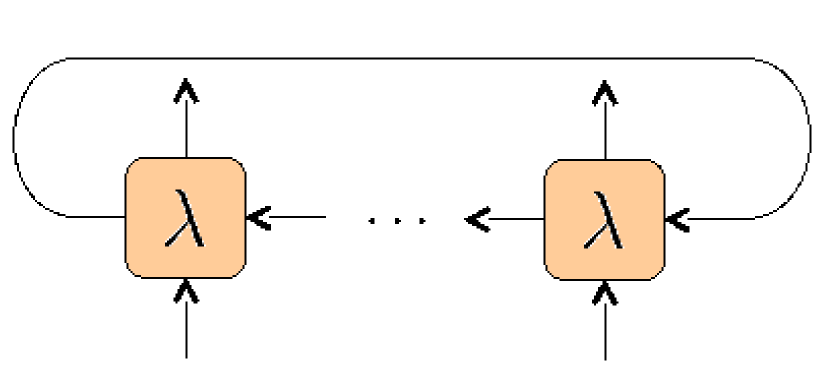
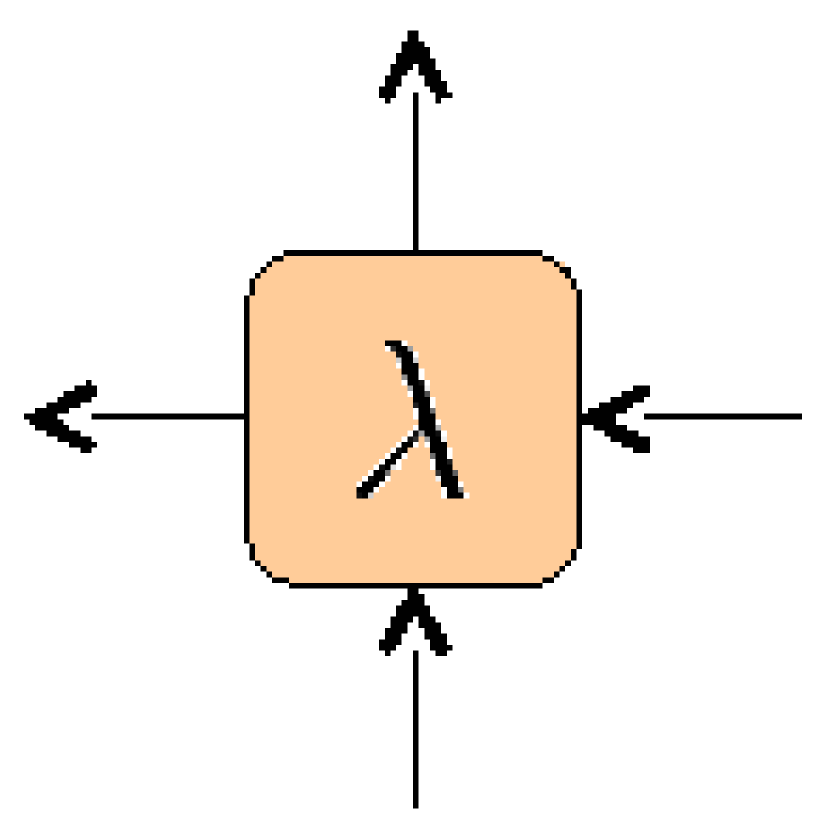
We represent each L𝐿L operator L(λ)αβab𝐿superscriptsubscript𝜆𝛼𝛽𝑎𝑏L(\lambda)_{\alpha\beta}^{ab} (a tensor with four indices) as shown in Fig. 1(a). We construct the transfer matrix TL(λ)=LL(λ)LL1(λ)L1(λ)subscript𝑇𝐿𝜆subscript𝐿𝐿𝜆subscript𝐿𝐿1𝜆subscript𝐿1𝜆T_{L}(\lambda)=L_{L}(\lambda)L_{L-1}(\lambda)\cdots L_{1}(\lambda) as shown in Fig. 1(b).
For the first level Bethe ansatz, the set of creation operators {C1,C2}subscript𝐶1subscript𝐶2\{C_{1},C_{2}\} in (29) is constructed by terminating the ends of the transfer matrix by boundary vectors/matrices as shown in Fig. 2. The boundary row vector (001)001(001) on the left selects the third row of the transfer matrix T(λ)𝑇𝜆T(\lambda). The matrix K𝐾K, which selects the first and second column of T(λ)𝑇𝜆T(\lambda), is defined as:

K=(100100)𝐾matrix100100\displaystyle\displaystyle K=\begin{pmatrix}1&0\\ 0&1\\ 0&0\end{pmatrix} (102)

We call the matrix K𝐾K the connector for it will be the bridge between the first level and nested Bethe ansatz.
For the nested Bethe ansatz, the creation operator C(1)(λ)superscript𝐶1𝜆C^{(1)}(\lambda) in (48) is constructed by terminating the ends of the transfer matrix by boundary vectors (0 1)01(0\;1) on the left and (1 0)superscript10(1\;0)^{\intercal} on the right (selecting the second row and first column respectively) as shown in Fig. 3.
Refer to caption
(a) L𝐿L operator L(λ)𝐿𝜆L(\lambda)
Refer to caption
(b) Monodromy matrix T(λ)𝑇𝜆T(\lambda)
Refer to caption
Figure 2: Creation operators {C1(λ),C2(λ)}subscript𝐶1𝜆subscript𝐶2𝜆\{C_{1}(\lambda),C_{2}(\lambda)\}
Refer to caption
Figure 3: Nested creation operator C(1)(λ)superscript𝐶1𝜆C^{(1)}(\lambda)

Now, we can construct the general tensor network form of the algebraic Bethe ansatz for both representations, as shown in Fig. 4,
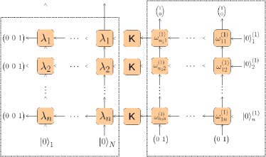
Refer to caption
Figure 4: Tensor Network representation

where we define:

ωab(1)=λa(1)λbsuperscriptsubscript𝜔𝑎𝑏1superscriptsubscript𝜆𝑎1subscript𝜆𝑏\displaystyle\omega_{ab}^{(1)}=\lambda_{a}^{(1)}-\lambda_{b} (103)
{n,n1}={{Ne,N},Lai representation{Nh+N,Nh},Sutherland representation𝑛subscript𝑛1casessubscript𝑁𝑒subscript𝑁Lai representationsubscript𝑁subscript𝑁subscript𝑁Sutherland representation\displaystyle\{n,n_{1}\}=\left\{\begin{array}[]{l l}\{N_{e},N_{\downarrow}\},&\textrm{Lai representation}\\ \{N_{h}+N_{\downarrow},N_{h}\},&\textrm{Sutherland representation}\end{array}\right. (106)

The tensor network is split into two main parts: the first level Bethe ansatz and the nested Bethe ansatz. The first level and the nested level are connected by contracting the indices a1,,ansubscript𝑎1subscript𝑎𝑛a_{1},\cdots,a_{n} of Caisubscript𝐶subscript𝑎𝑖C_{a_{i}} of the creation operators in the first level with the wavefunction of the nested level, as shown in (40). The matrix K𝐾K in Fig. 4 (as defined in (102)) selects the two first level creation operators {C1,C2}subscript𝐶1subscript𝐶2\{C_{1},C_{2}\} and connects them to the corresponding index of the wavefunction in the nested Bethe ansatz.

The bond dimension of each bond in the tensor network for the first level Bethe ansatz is 333, while that for the nested level is 222. Due to the fact that Caisubscript𝐶subscript𝑎𝑖C_{a_{i}} are creation operators, …

IV Grading in terms of tensor networks

In this section, we explicitly consider the grading for both representations in detail. The tensor product is graded by assigning Grassmann parities to the basis vectors, which represents the fermionic nature of the t-J model. This introduces minus signs which are shown explicitly in (30) and (87). These minus signs are non-local at first glance, as the exponent of the minus sign of each element in the monodromy matrix depends on the parities of the indices to its right. However, in order to perform the approximate contraction of the tensor network (described in Sec. V) in a sequential manner, we have to localize these minus signs. We have devised two ways to do this as described in the following.

IV.1 Method 1

In this method we shall write the monodromy matrices in a recursive form such that the minus signs are included locally in the L𝐿L operators. Using such a representation in the form of matrices allows us to contract the tensor network efficiently, especially in languages like Matlab which matrix computations are designed for speed.

IV.1.1 Lai representation

In Lai representation, the graded tensor products in the first level Bethe ansatz produce non-local minus signs as shown in (30). However, since the nested Bethe ansatz consist of a system of two fermions (in which the minus signs cancel), the graded tensor products do not produce any explicit (non-local) minus signs.

We introduce the following notation:

εk=ϵαk+ϵβksubscript𝜀𝑘subscriptitalic-ϵsubscript𝛼𝑘subscriptitalic-ϵsubscript𝛽𝑘\displaystyle\varepsilon_{k}=\epsilon_{\alpha_{k}}+\epsilon_{\beta_{k}} (107)
Lk(λ)αkβkab|εk=y=Lk(λ)αkβkabδεk,y,y=0,1formulae-sequenceevaluated-atsubscript𝐿𝑘superscriptsubscript𝜆subscript𝛼𝑘subscript𝛽𝑘𝑎𝑏subscript𝜀𝑘𝑦subscript𝐿𝑘superscriptsubscript𝜆subscript𝛼𝑘subscript𝛽𝑘𝑎𝑏subscript𝛿subscript𝜀𝑘𝑦𝑦01\displaystyle\left.L_{k}(\lambda)_{\alpha_{k}\beta_{k}}^{ab}\right|_{\varepsilon_{k}=y}=L_{k}(\lambda)_{\alpha_{k}\beta_{k}}^{ab}\delta_{\varepsilon_{k},y},\qquad y=0,1 (108)

The delta function picks out only the quantum operators of the desired Grassmann parity (εk=0 or 1subscript𝜀𝑘0 or 1\varepsilon_{k}=0\textrm{ or }1). In Lai representation, the fermionic (εk=1subscript𝜀𝑘1\varepsilon_{k}=1) operators are Casubscript𝐶𝑎C_{a} and Bbsubscript𝐵𝑏B_{b} in (29) (a,b=1,2formulae-sequence𝑎𝑏12a,b=1,2), and the rest are bosonic (εk=0subscript𝜀𝑘0\varepsilon_{k}=0). The original L𝐿L operator is simply expressed by Lk(λ)=Lk(λ)|εk=0+Lk(λ)|εk=1subscript𝐿𝑘𝜆evaluated-atsubscript𝐿𝑘𝜆subscript𝜀𝑘0evaluated-atsubscript𝐿𝑘𝜆subscript𝜀𝑘1L_{k}(\lambda)=\left.L_{k}(\lambda)\right|_{\varepsilon_{k}=0}+\left.L_{k}(\lambda)\right|_{\varepsilon_{k}=1}. We define the following primed L𝐿L operator and monodromy matrix:

Lk(λ)αβab=Lk(λ)αβab(1)ϵαsubscriptsuperscript𝐿𝑘superscriptsubscript𝜆𝛼𝛽𝑎𝑏subscript𝐿𝑘superscriptsubscript𝜆𝛼𝛽𝑎𝑏superscript1subscriptitalic-ϵ𝛼\displaystyle L^{\prime}_{k}(\lambda)_{\alpha\beta}^{ab}=L_{k}(\lambda)_{\alpha\beta}^{ab}(-1)^{\epsilon_{\alpha}} (109)
{[TL(λ)]ab}α1αLβ1βL=LL(λ)αLβLacLLL1(λ)αL1βL1cLcL1L1(λ)α1β1c2c1(1)j=2L(ϵαj+ϵβj)i=1j1ϵαisubscriptsuperscriptdelimited-[]superscriptsubscript𝑇𝐿𝜆𝑎𝑏subscript𝛼1subscript𝛼𝐿subscript𝛽1subscript𝛽𝐿superscriptsubscript𝐿𝐿subscriptsuperscript𝜆𝑎subscript𝑐𝐿subscript𝛼𝐿subscript𝛽𝐿superscriptsubscript𝐿𝐿1subscriptsuperscript𝜆subscript𝑐𝐿subscript𝑐𝐿1subscript𝛼𝐿1subscript𝛽𝐿1superscriptsubscript𝐿1subscriptsuperscript𝜆subscript𝑐2subscript𝑐1subscript𝛼1subscript𝛽1superscript1superscriptsubscript𝑗2𝐿subscriptitalic-ϵsubscript𝛼𝑗subscriptitalic-ϵsubscript𝛽𝑗superscriptsubscript𝑖1𝑗1subscriptitalic-ϵsubscript𝛼𝑖\displaystyle\{[T_{L}^{\prime}(\lambda)]^{ab}\}_{\begin{subarray}{c}\alpha_{1}\cdots\alpha_{L}\\ \beta_{1}\cdots\beta_{L}\end{subarray}}=L_{L}^{\prime}(\lambda)^{ac_{L}}_{\alpha_{L}\beta_{L}}L_{L-1}^{\prime}(\lambda)^{{c_{L}}{c_{L-1}}}_{\alpha_{L-1}\beta_{L-1}}\cdots L_{1}^{\prime}(\lambda)^{c_{2}c_{1}}_{\alpha_{1}\beta_{1}}(-1)^{\sum_{j=2}^{L}(\epsilon_{\alpha_{j}}+\epsilon_{\beta_{j}})\sum_{i=1}^{j-1}\epsilon_{\alpha_{i}}} (110)

Now, we can write (30) in a recursive form that allows the minus signs to be localized:

({[Tk+1(λ)]ab}α1αk+1β1βk+1{[Tk+1(λ)]ab}α1αk+1β1βk+1)=(Lk+1(λ)αk+1βk+1ack+1|εk+1=0Lk+1(λ)αk+1βk+1ack+1|εk+1=1Lk+1(λ)αk+1βk+1ack+1|εk+1=1Lk+1(λ)αk+1βk+1ack+1|εk+1=0)({[Tk(λ)]ck+1b}α1αkβ1βk{[Tk(λ)]ck+1b}α1αkβ1βk)matrixsubscriptsuperscriptdelimited-[]subscript𝑇𝑘1𝜆𝑎𝑏subscript𝛼1subscript𝛼𝑘1subscript𝛽1subscript𝛽𝑘1subscriptsuperscriptdelimited-[]superscriptsubscript𝑇𝑘1𝜆𝑎𝑏subscript𝛼1subscript𝛼𝑘1subscript𝛽1subscript𝛽𝑘1matrixevaluated-atsubscript𝐿𝑘1superscriptsubscript𝜆subscript𝛼𝑘1subscript𝛽𝑘1𝑎subscript𝑐𝑘1subscript𝜀𝑘10evaluated-atsubscript𝐿𝑘1superscriptsubscript𝜆subscript𝛼𝑘1subscript𝛽𝑘1𝑎subscript𝑐𝑘1subscript𝜀𝑘11evaluated-atsuperscriptsubscript𝐿𝑘1superscriptsubscript𝜆subscript𝛼𝑘1subscript𝛽𝑘1𝑎subscript𝑐𝑘1subscript𝜀𝑘11evaluated-atsuperscriptsubscript𝐿𝑘1superscriptsubscript𝜆subscript𝛼𝑘1subscript𝛽𝑘1𝑎subscript𝑐𝑘1subscript𝜀𝑘10matrixsubscriptsuperscriptdelimited-[]subscript𝑇𝑘𝜆subscript𝑐𝑘1𝑏subscript𝛼1subscript𝛼𝑘subscript𝛽1subscript𝛽𝑘subscriptsuperscriptdelimited-[]superscriptsubscript𝑇𝑘𝜆subscript𝑐𝑘1𝑏subscript𝛼1subscript𝛼𝑘subscript𝛽1subscript𝛽𝑘\displaystyle\displaystyle\begin{pmatrix}\{[T_{k+1}(\lambda)]^{ab}\}_{\begin{subarray}{c}\alpha_{1}\cdots\alpha_{k+1}\\ \beta_{1}\cdots\beta_{k+1}\end{subarray}}\\ \{[T_{k+1}^{\prime}(\lambda)]^{ab}\}_{\begin{subarray}{c}\alpha_{1}\cdots\alpha_{k+1}\\ \beta_{1}\cdots\beta_{k+1}\end{subarray}}\end{pmatrix}=\begin{pmatrix}\left.L_{k+1}(\lambda)_{\alpha_{k+1}\beta_{k+1}}^{ac_{k+1}}\right|_{\varepsilon_{k+1}=0}&\left.L_{k+1}(\lambda)_{\alpha_{k+1}\beta_{k+1}}^{ac_{k+1}}\right|_{\varepsilon_{k+1}=1}\\ \left.L_{k+1}^{\prime}(\lambda)_{\alpha_{k+1}\beta_{k+1}}^{ac_{k+1}}\right|_{\varepsilon_{k+1}=1}&\left.L_{k+1}^{\prime}(\lambda)_{\alpha_{k+1}\beta_{k+1}}^{ac_{k+1}}\right|_{\varepsilon_{k+1}=0}\\ \end{pmatrix}\begin{pmatrix}\{[T_{k}(\lambda)]^{c_{k+1}b}\}_{\begin{subarray}{c}\alpha_{1}\cdots\alpha_{k}\\ \beta_{1}\cdots\beta_{k}\end{subarray}}\\ \{[T_{k}^{\prime}(\lambda)]^{c_{k+1}b}\}_{\begin{subarray}{c}\alpha_{1}\cdots\alpha_{k}\\ \beta_{1}\cdots\beta_{k}\end{subarray}}\end{pmatrix} (111)

The minus signs are absorbed locally into the definition of Lk(λ)subscriptsuperscript𝐿𝑘𝜆L^{\prime}_{k}(\lambda). The L𝐿L operators are now embedded in a larger matrix space, which we call the external matrix space. To use this construction to handle the grading, we would have to alter our tensor network so to include the external matrix space.
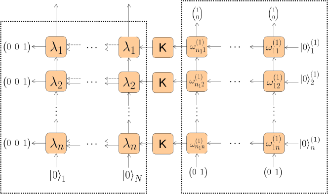
Refer to caption
Figure 5: Graded Tensor Network for Lai representation

Ksuperscript𝐾K^{\prime} is defined as:

K=(11)(100100)superscript𝐾tensor-productmatrix11matrix100100\displaystyle\displaystyle K^{\prime}=\begin{pmatrix}1\\ 1\end{pmatrix}\otimes\begin{pmatrix}1&0\\ 0&1\\ 0&0\end{pmatrix} (112)

The boundary vectors on the left of Fig. 5 and Ksuperscript𝐾K^{\prime} live in the space V(0|2)V(1|2)tensor-productsuperscript𝑉conditional02superscript𝑉conditional12V^{(0|2)}\otimes V^{(1|2)}, where the first space V(0|2)superscript𝑉conditional02V^{(0|2)} is the external matrix space and the second space V(1|2)superscript𝑉conditional12V^{(1|2)} is the matrix space.

IV.1.2 Sutherland representation

For Sutherland representation, the graded tensor products in both the first level and nested Bethe ansatz produce minus signs. The minus signs produced by the tensor product in the first level Bethe ansatz is exactly the same as in Lai representation as shown in (30). However, due to the choice of grading in Sutherland representation, the fermionic (εk=1subscript𝜀𝑘1\varepsilon_{k}=1) operators are B1subscript𝐵1B_{1}, C1subscript𝐶1C_{1}, A12subscript𝐴12A_{12} and A21subscript𝐴21A_{21} in (29), and the rest are bosonic (εk=0subscript𝜀𝑘0\varepsilon_{k}=0). Nevertheless, the form of the recursion relation of the first level monodromy matrix for Sutherland representation is exactly the same as (111) in Lai representation.

Now, for the graded tensor product (87) in the nested Bethe ansatz, we introduce the following:

Lk(1)(λ)αβab=Lk(1)(λ)αβab(1)ϵαsubscriptsuperscript𝐿1𝑘superscriptsubscript𝜆𝛼𝛽𝑎𝑏superscriptsubscript𝐿𝑘1superscriptsubscript𝜆𝛼𝛽𝑎𝑏superscript1subscriptitalic-ϵ𝛼\displaystyle L^{(1)\prime}_{k}(\lambda)_{\alpha\beta}^{ab}=L_{k}^{(1)}(\lambda)_{\alpha\beta}^{ab}(-1)^{\epsilon_{\alpha}} (113)
{[TL(1)(λ)]ab}α1αLβ1βL=LL(1)(λ)αLβLacLLL1(1)(λ)αL1βL1cLcL1L1(1)(λ)α1β1c2c1(1)j=2L(ϵαj+ϵβj)i=1j1(ϵαi+1)subscriptsuperscriptdelimited-[]superscriptsubscript𝑇𝐿1𝜆𝑎𝑏subscript𝛼1subscript𝛼𝐿subscript𝛽1subscript𝛽𝐿superscriptsubscript𝐿𝐿1subscriptsuperscript𝜆𝑎subscript𝑐𝐿subscript𝛼𝐿subscript𝛽𝐿superscriptsubscript𝐿𝐿11subscriptsuperscript𝜆subscript𝑐𝐿subscript𝑐𝐿1subscript𝛼𝐿1subscript𝛽𝐿1superscriptsubscript𝐿11subscriptsuperscript𝜆subscript𝑐2subscript𝑐1subscript𝛼1subscript𝛽1superscript1superscriptsubscript𝑗2𝐿subscriptitalic-ϵsubscript𝛼𝑗subscriptitalic-ϵsubscript𝛽𝑗superscriptsubscript𝑖1𝑗1subscriptitalic-ϵsubscript𝛼𝑖1\displaystyle\{[T_{L}^{(1)\prime}(\lambda)]^{ab}\}_{\begin{subarray}{c}\alpha_{1}\cdots\alpha_{L}\\ \beta_{1}\cdots\beta_{L}\end{subarray}}=L_{L}^{(1)\prime}(\lambda)^{ac_{L}}_{\alpha_{L}\beta_{L}}L_{L-1}^{(1)\prime}(\lambda)^{{c_{L}}{c_{L-1}}}_{\alpha_{L-1}\beta_{L-1}}\cdots L_{1}^{(1)\prime}(\lambda)^{c_{2}c_{1}}_{\alpha_{1}\beta_{1}}(-1)^{\sum_{j=2}^{L}(\epsilon_{\alpha_{j}}+\epsilon_{\beta_{j}})\sum_{i=1}^{j-1}(\epsilon_{\alpha_{i}}+1)} (114)

Now, we can write (87) in a recursive form that allows the minus signs to be localized:

({[Tk+1(1)(λ)]ab}α1αk+1β1βk+1{[Tk+1(1)(λ)]ab}α1αk+1β1βk+1)=(Lk+1(1)(λ)αk+1βk+1ack+1|εk+1=0Lk+1(1)(λ)αk+1βk+1ack+1|εk+1=1Lk+1(1)(λ)αk+1βk+1ack+1|εk+1=1Lk+1(1)(λ)αk+1βk+1ack+1|εk+1=0)({[Tk(1)(λ)]ck+1b}α1αkβ1βk{[Tk(1)(λ)]ck+1b}α1αkβ1βk)matrixsubscriptsuperscriptdelimited-[]superscriptsubscript𝑇𝑘11𝜆𝑎𝑏subscript𝛼1subscript𝛼𝑘1subscript𝛽1subscript𝛽𝑘1subscriptsuperscriptdelimited-[]superscriptsubscript𝑇𝑘11𝜆𝑎𝑏subscript𝛼1subscript𝛼𝑘1subscript𝛽1subscript𝛽𝑘1matrixevaluated-atsuperscriptsubscript𝐿𝑘11superscriptsubscript𝜆subscript𝛼𝑘1subscript𝛽𝑘1𝑎subscript𝑐𝑘1subscript𝜀𝑘10evaluated-atsuperscriptsubscript𝐿𝑘11superscriptsubscript𝜆subscript𝛼𝑘1subscript𝛽𝑘1𝑎subscript𝑐𝑘1subscript𝜀𝑘11evaluated-atsuperscriptsubscript𝐿𝑘11superscriptsubscript𝜆subscript𝛼𝑘1subscript𝛽𝑘1𝑎subscript𝑐𝑘1subscript𝜀𝑘11evaluated-atsuperscriptsubscript𝐿𝑘11superscriptsubscript𝜆subscript𝛼𝑘1subscript𝛽𝑘1𝑎subscript𝑐𝑘1subscript𝜀𝑘10matrixsubscriptsuperscriptdelimited-[]superscriptsubscript𝑇𝑘1𝜆subscript𝑐𝑘1𝑏subscript𝛼1subscript𝛼𝑘subscript𝛽1subscript𝛽𝑘subscriptsuperscriptdelimited-[]superscriptsubscript𝑇𝑘1𝜆subscript𝑐𝑘1𝑏subscript𝛼1subscript𝛼𝑘subscript𝛽1subscript𝛽𝑘\displaystyle\displaystyle\begin{pmatrix}\{[T_{k+1}^{(1)}(\lambda)]^{ab}\}_{\begin{subarray}{c}\alpha_{1}\cdots\alpha_{k+1}\\ \beta_{1}\cdots\beta_{k+1}\end{subarray}}\\ \{[T_{k+1}^{(1)\prime}(\lambda)]^{ab}\}_{\begin{subarray}{c}\alpha_{1}\cdots\alpha_{k+1}\\ \beta_{1}\cdots\beta_{k+1}\end{subarray}}\end{pmatrix}=\begin{pmatrix}\left.L_{k+1}^{(1)}(\lambda)_{\alpha_{k+1}\beta_{k+1}}^{ac_{k+1}}\right|_{\varepsilon_{k+1}=0}&\left.L_{k+1}^{(1)}(\lambda)_{\alpha_{k+1}\beta_{k+1}}^{ac_{k+1}}\right|_{\varepsilon_{k+1}=1}\\ \left.L_{k+1}^{(1)\prime}(\lambda)_{\alpha_{k+1}\beta_{k+1}}^{ac_{k+1}}\right|_{\varepsilon_{k+1}=1}&\left.L_{k+1}^{(1)\prime}(\lambda)_{\alpha_{k+1}\beta_{k+1}}^{ac_{k+1}}\right|_{\varepsilon_{k+1}=0}\\ \end{pmatrix}\begin{pmatrix}\{[T_{k}^{(1)}(\lambda)]^{c_{k+1}b}\}_{\begin{subarray}{c}\alpha_{1}\cdots\alpha_{k}\\ \beta_{1}\cdots\beta_{k}\end{subarray}}\\ \{[T_{k}^{(1)\prime}(\lambda)]^{c_{k+1}b}\}_{\begin{subarray}{c}\alpha_{1}\cdots\alpha_{k}\\ \beta_{1}\cdots\beta_{k}\end{subarray}}\end{pmatrix} (115)

The minus signs in the nested Bethe ansatz are absorbed locally into the definition of Lk(1)(λ)subscriptsuperscript𝐿1𝑘𝜆L^{(1)\prime}_{k}(\lambda). To use this construction to handle the grading, we would have to alter our tensor network so to include the external matrix space (in both the first level and nested Bethe ansatz for Sutherland representation).
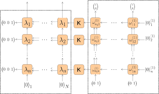
Refer to caption
Figure 6: Graded Tensor Network for Sutherland representation

The boundary vectors on the left of Fig. 6 and Ksuperscript𝐾K^{\prime} live in the space V(1|1)V(1|2)tensor-productsuperscript𝑉conditional11superscript𝑉conditional12V^{(1|1)}\otimes V^{(1|2)}, where the first space V(1|1)superscript𝑉conditional11V^{(1|1)} is the external matrix space and the second space V(1|2)superscript𝑉conditional12V^{(1|2)} is the matrix space, of the first level L(1)superscript𝐿1L^{(1)} operators. The boundary vectors to the top and bottom of the nested Bethe ansatz live similarly in the space V(1|1)V(1|1)tensor-productsuperscript𝑉conditional11superscript𝑉conditional11V^{(1|1)}\otimes V^{(1|1)}, where the first space is the external matrix space and the second space is the matrix space, of the nested L(1)superscript𝐿1L^{(1)} operators.

IV.2 Method 2

IV.2.1 Lai representation

In Lai representation, the grading of the first level Bethe network can also be handled by adding an extra bond that carries the parity information of the indices, denoted by the dotted lines in Fig. 5. The parity bond pmsubscript𝑝𝑚p_{m} at the mthsuperscript𝑚𝑡m^{th} site satisfies the relation pm=pm1+ϵkm(mod 2)subscript𝑝𝑚subscript𝑝𝑚1subscriptitalic-ϵsubscript𝑘𝑚mod 2p_{m}=p_{m-1}+\epsilon_{k_{m}}\,(\textrm{mod 2}), where p0=0subscript𝑝00p_{0}=0. In addition, these parity bonds, which store local information about the minus signs of (30), satisfy the recursive relation

(1)j=2m(ϵkj+ϵlj)i=1j1ϵkisuperscript1superscriptsubscript𝑗2𝑚subscriptitalic-ϵsubscript𝑘𝑗subscriptitalic-ϵsubscript𝑙𝑗superscriptsubscript𝑖1𝑗1subscriptitalic-ϵsubscript𝑘𝑖\displaystyle\displaystyle(-1)^{\sum_{j=2}^{m}(\epsilon_{k_{j}}+\epsilon_{l_{j}})\sum_{i=1}^{j-1}\epsilon_{k_{i}}} =(1)j=2m1(ϵkj+ϵlj)i=1j1ϵkiabsentsuperscript1superscriptsubscript𝑗2𝑚1subscriptitalic-ϵsubscript𝑘𝑗subscriptitalic-ϵsubscript𝑙𝑗superscriptsubscript𝑖1𝑗1subscriptitalic-ϵsubscript𝑘𝑖\displaystyle=(-1)^{\sum_{j=2}^{m-1}(\epsilon_{k_{j}}+\epsilon_{l_{j}})\sum_{i=1}^{j-1}\epsilon_{k_{i}}}
×(1)(ϵkm+ϵlm)pmabsentsuperscript1subscriptitalic-ϵsubscript𝑘𝑚subscriptitalic-ϵsubscript𝑙𝑚subscript𝑝𝑚\displaystyle\;\;\;\;\times(-1)^{(\epsilon_{k_{m}}+\epsilon_{l_{m}})p_{m}} (116)

As such, in the tensor network picture with grading, each L𝐿L operator Lmsubscript𝐿𝑚L_{m} becomes a tensor with 666 indices: 222 horizontal indices of dimension 333 describing the matrix space, 222 vertical indices kmsubscript𝑘𝑚k_{m} and lmsubscript𝑙𝑚l_{m} of dimension 333 describing the physical space and 222 parity indices pm1subscript𝑝𝑚1p_{m-1} and pmsubscript𝑝𝑚p_{m} of dimension 222. Because of the recursive relation (116), the nonlocal minus signs of (30) can be reproduced by multiplying each L𝐿L operator with (1)(ϵkm+ϵlm)pmsuperscript1subscriptitalic-ϵsubscript𝑘𝑚subscriptitalic-ϵsubscript𝑙𝑚subscript𝑝𝑚(-1)^{(\epsilon_{k_{m}}+\epsilon_{l_{m}})p_{m}}.

IV.2.2 Sutherland representation

In Sutherland representation, both the first and the nested level Bethe network are graded, and they are handled by adding an extra bond that carries the parity information of the indices, denoted by the dotted lines in both levels of the Bethe ansatz in Fig. 6. As before, the parity bond pmsubscript𝑝𝑚p_{m} at the mthsuperscript𝑚𝑡m^{th} site satisfies the relation pm=pm1+ϵkm(mod 2)subscript𝑝𝑚subscript𝑝𝑚1subscriptitalic-ϵsubscript𝑘𝑚mod 2p_{m}=p_{m-1}+\epsilon_{k_{m}}\,(\textrm{mod 2}), where p0=0subscript𝑝00p_{0}=0, such that the minus signs of (30) can be localized.

IV.3 Equivalence of the two methods

Upon joining the additional parity bonds (of dimension 222) in the second method with the bonds in the matrix space (of dimension 333) of the original tensor network, the L𝐿L operators are now tensors of 666 by 666 in the matrix space and 333 by 333 in the physical space, which has the same dimensions as that of the L𝐿L operators of the first method. These two methods will then give rise to exactly the same tensor network, producing equivalent tensors (up to a unitary transformation). The first method can thus be simply considered as an explicit formulation of the joining of the parity bonds with the original bonds in the matrix space in the second method.

V Approximate contraction of the tensor network
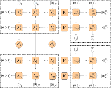
Refer to caption
Figure 7: Tensor Network calculation of expectation values

The calculation of expectation values with respect to a Bethe eigenstate of the form of (40) is a considerably complex problem, because it requires the contraction of the tensor network depicted in Fig. 7. A tensor network with such a structure also appears in connection with the calculation of partition functions of two-dimensional classical systems and one-dimensional quantum systems and the calculation of expectation values with respect to PEPSs. The complexity of contracting this network scales exponentially with the number of rows M𝑀M or columns N𝑁N (depending on the direction of contraction), which renders exact calculations infeasible.

Following Murg et al.Murg et al. (2012), to circumvent this problem, we attempt to perform the contraction in an approximative numerical way: the main idea is to consider the network in Fig. 4 as the time evolution of MPOs (L𝐿L operators) acting on MPSs in a sequential order. After each evolution step, the state remains an MPS, but the virtual dimension is increased, by a factor of 333 (first level) or 222 (nested level). Thus, we approximate the MPS after each evolution step by a MPS with smaller virtual dimension. Of course, we must exercise caution, as the creation operators are not unitary and the intermediate states of the evolution can be nonphysical (i.e., they might have to be represented by an MPS with high virtual dimension). We choose the order of contraction to be such:

  1. 1.

    In the nested Bethe ansatz, act the n1subscript𝑛1n_{1} nested creation operators C(1)(λn1(1))C(1)(λ1(1))superscript𝐶1superscriptsubscript𝜆subscript𝑛11superscript𝐶1superscriptsubscript𝜆11C^{(1)}(\lambda_{n_{1}}^{(1)})\cdots C^{(1)}(\lambda_{1}^{(1)}) on the initial MPS |0(1)superscriptket01\left|{0}\right\rangle^{(1)} sequentially, contracting approximately to get an MPS at each step, to produce a boundary MPS on the right of the first level Bethe ansatz.

  2. 2.

    Now, in the first level Bethe ansatz, n𝑛n first level creation operators C(λn)C(λ1)𝐶subscript𝜆𝑛𝐶subscript𝜆1C(\lambda_{n})\cdots C(\lambda_{1}) on the initial MPS |0ket0\left|{0}\right\rangle sequentially, contracting approximately to get an MPS at each step, with the right end of the first level Bethe ansatz terminated by the boundary MPS produced in the first step.

At each step in the above contraction process, we let

|Ψm=Cam(λm)|Ψ~m1,m=1,,nformulae-sequenceketsubscriptΨ𝑚subscript𝐶subscript𝑎𝑚subscript𝜆𝑚ketsubscript~Ψ𝑚1𝑚1𝑛\displaystyle\left|{\Psi_{m}}\right\rangle=C_{a_{m}}(\lambda_{m})\left|{\tilde{\Psi}_{m-1}}\right\rangle,\,\,m=1,\cdots,n (117)
|Ψm1(1)=C(1)(λm1(1))|Ψ~m11(1),m1=1,,n1formulae-sequencesuperscriptketsubscriptΨsubscript𝑚11superscript𝐶1superscriptsubscript𝜆subscript𝑚11ketsuperscriptsubscript~Ψsubscript𝑚111subscript𝑚11subscript𝑛1\displaystyle\left|{\Psi_{m_{1}}}\right\rangle^{(1)}=C^{(1)}(\lambda_{m_{1}}^{(1)})\left|{\tilde{\Psi}_{m_{1}-1}^{(1)}}\right\rangle,\,\,m_{1}=1,\cdots,n_{1} (118)

where

|Ψ~0=|0,|Ψ~0(1)=|0(1)formulae-sequenceketsubscript~Ψ0ket0superscriptketsubscript~Ψ01superscriptket01\displaystyle\displaystyle\left|{\tilde{\Psi}_{0}}\right\rangle=\left|{0}\right\rangle,\quad\left|{\tilde{\Psi}_{0}}\right\rangle^{(1)}=\left|{0}\right\rangle^{(1)} (119)

At each step of the first level Bethe ansatz, |ΨmketsubscriptΨ𝑚\left|{\Psi_{m}}\right\rangle is approximated by the MPS |Ψ~mketsubscript~Ψ𝑚\left|{\tilde{\Psi}_{m}}\right\rangle that has maximal bond dimension D𝐷D and is closest to |Ψ~mketsubscript~Ψ𝑚\left|{\tilde{\Psi}_{m}}\right\rangle. In other words, we try solve the minimization problem

K:=|Ψm|Ψ~m2minassign𝐾superscriptnormketsubscriptΨ𝑚ketsubscript~Ψ𝑚2min\displaystyle\displaystyle K:=\left\|\left|{\Psi_{m}}\right\rangle-\left|{\tilde{\Psi}_{m}}\right\rangle\right\|^{2}\rightarrow\textrm{min} (120)

by optimizing over all matrices of the MPS |Ψ~mketsubscript~Ψ𝑚\left|{\tilde{\Psi}_{m}}\right\rangle. (This minimization is done in the same manner for the nested Bethe ansatz.) This minimization problem also appears in the context of numerical calculation of expectation values with respect to PEPSs, calculation of partition functions, and (imaginary) time evolution of one-dimensional quantum systems. In this way, the MPS approximation of the Bethe state is obtained for the whole tensor network. The error of the approximation is well controlled in the sense that the expectation value of the energy can always be calculated with respect to the approximated MPS |Ψ~mketsubscript~Ψ𝑚\left|{\tilde{\Psi}_{m}}\right\rangle and compared to the exact energy available from the Bethe ansatz.

There is a (mathematical) degree of freedom that can be used to improve the approximation. This degree of freedom is due to the fact that the set of {{λ},{λ(1)}}𝜆superscript𝜆1\{\{\lambda\},\{\lambda^{(1)}\}\} encode information about physical quantities and the ordering of the them should not change the final wavefunction produced. That is, permutation of order of applying the creation operators through permutation of the set of {{λ},{λ(1)}}𝜆superscript𝜆1\{\{\lambda\},\{\lambda^{(1)}\}\} will not change the final wavefunction. However, the intermediate states are a priori not physical ground states; i.e., there is no reason for them to lie in the set of MPS with low bond dimension. Even so, similar to that which is noted in Murg et al. (2012), there is always an ordering of the set of λ𝜆\lambda’s such that the intermediate states contain as little entanglement as possible. We then use that ordering for doing the approximation.

VI Numerical Results

Using the previously described method, we have obtained numerical results for the t-J model with periodic boundary conditions. We chose to implement the tensor network representation of the Sutherland representation, since, near half filling, its Bethe ansatz equations are more well behaved numerically, and its tensor network is smaller. We chose to use the first method of implementing grading as the explicit construction of the matrices is more easily checked for errors. As a proof of principle, we obtain the correlation functions of eigenstates on lattices of length 181818 as presented below. Calculations for lattices of larger length can be achieved through consideration of symmetries, or using mathematical packages which can extend the limit of machine precision.

VI.1 Electron correlator
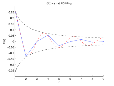
Refer to caption
Figure 8: Spin-up correlator at 2/3 filling for ground state

The asymptotic behavior of the spin correlator is predicted by conformal field theory to be

Gσ(r)=cσ(r)cσ(0)rηcos(kFr)subscript𝐺𝜎𝑟delimited-⟨⟩superscriptsubscript𝑐𝜎𝑟subscript𝑐𝜎0proportional-tosuperscript𝑟𝜂𝑐𝑜𝑠subscript𝑘𝐹𝑟\displaystyle\displaystyle G_{\sigma}(r)=\left\langle c_{\sigma}^{\dagger}(r)c_{\sigma}(0)\right\rangle\propto r^{-\eta}cos(k_{F}r) (121)

where η𝜂\eta and kFsubscript𝑘𝐹k_{F} are as defined in Kawakami and Yang (1991). This is strongly supported by our results, as can be gathered from Fig. 8.

VI.2 Singlet pair superconducting correlators
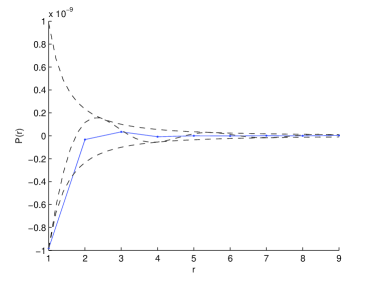
Refer to caption
Figure 9: Singlet pair superconducting correlator at 2/3 filling for ground state

The asymptotic behavior of the singlet pair correlator is predicted by conformal field theory to be

Ps(r)c(r+1)c(r)c(1)c(0)rβscos(2kFr)proportional-tosubscript𝑃𝑠𝑟delimited-⟨⟩superscriptsubscript𝑐𝑟1superscriptsubscript𝑐𝑟subscript𝑐1subscript𝑐0superscript𝑟subscript𝛽𝑠𝑐𝑜𝑠2subscript𝑘𝐹𝑟\displaystyle\displaystyle P_{s}(r)\left\langle c_{\uparrow}^{\dagger}(r+1)c_{\downarrow}^{\dagger}(r)c_{\uparrow}(1)c_{\downarrow}(0)\right\rangle\propto r^{-\beta_{s}}cos(2k_{F}r) (122)

where βssubscript𝛽𝑠\beta_{s} and kFsubscript𝑘𝐹k_{F} are as defined in Kawakami and Yang (1991). This is strongly supported by our results, as can be gathered from Fig. 9.

VI.3 Spin correlator

Refer to caption
Figure 10: Spin correlator at various filling for charge triplet state - the number in the legend shows N𝑁N, the total number of particles

The spin correlator is defined as:

χ(r)=Sz(r)Sz(0),Sz(r)=(n(r)n(r))formulae-sequence𝜒𝑟delimited-⟨⟩subscript𝑆𝑧𝑟subscript𝑆𝑧0subscript𝑆𝑧𝑟subscript𝑛𝑟subscript𝑛𝑟\displaystyle\displaystyle\chi(r)=\left\langle S_{z}(r)S_{z}(0)\right\rangle\;\;,\;\;S_{z}(r)=(n_{\uparrow}(r)-n_{\downarrow}(r)) (123)

We consider the charge triplet state and calculate its spin correlator, as shown in Fig. 10. It shows that an interesting trend that as we increase the filling towards half filling, the variation of the spin correlator increases, and that it tends toward a zigzag pattern that alternates between the even and odd lattice sites at half filling.

VI.4 Charge density correlator
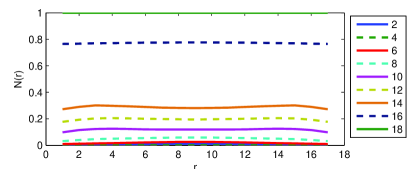
Refer to caption
Figure 11: Charge density correlator at various filling for charge triplet state (color online) - the number in the legend shows N, the total number of particles
Refer to caption
Figure 12: Normalized charge density correlator at various filling for charge triplet state (color online) - the number in the legend shows N𝑁N, the total number of particles

The charge density correlator is defined as:

N(r)=n(r)n(0),n(r)=(n(r)+n(r))formulae-sequence𝑁𝑟delimited-⟨⟩𝑛𝑟𝑛0𝑛𝑟subscript𝑛𝑟subscript𝑛𝑟\displaystyle\displaystyle N(r)=\left\langle n(r)n(0)\right\rangle\;\;,\;\;n(r)=(n_{\uparrow}(r)+n_{\downarrow}(r)) (124)

We consider the charge triplet state and calculate its charge density correlator, as shown in Fig. 11. It does not fully show the trend of variation across the lattice sites, as it is dominated by the constant term in the correlator. As such, we attempt to “normalize” the correlator by setting the correlator of the first site to be zero (by translation), as shown in Fig. 12. This clearly shows a trend that as N𝑁N (total number of particles) increases, the magnitude of the variation of the correlator across the lattice sites increases, until N=14𝑁14N=14 which is reaches a peak, then decreases.

VII Conclusions

Summing up, we have presented a method for approximative calculation of expectation values with respect to Bethe eigenstates of the t-J model. To achieve this, we make use of the fact that a Bethe eigenstate is a product of MPOs applied to an MPS. We systematically reduce the virtual dimension after each multiplication and obtain an MPS with small virtual dimension that can be used for the calculation of any expectation value. As a proof of principle, we have obtained the correlation functions of eigenstates on finite length lattices with our method.

Acknowledgements.
V. M. and F. V. acknowledge support from the SFB projects FoQuS and ViCoM, the European projects Quevadis, and the ERC grant Querg. V. E. K. and Y. Q. C. acknowledge support from the NSF grant DMS-1205422.

References

  • Bethe (1931) H. Bethe, Z. Phys. 71, 205 (1931)
  • Foerster and Karowski (1993) A. Foerster and M. Karowski, Nuclear Physics B 396, 611 (1993)
  • Essler and Korepin (1992) F. H. Essler and V. E. Korepin, Physical Review B 46, 9147 (1992)
  • Essler et al. (2005) F. H. L. Essler, H. Frahm, F. Göhmann, A. Klümper,  and V. E. Korepin, The one-dimensional Hubbard model (Cambridge University Press, 2005)
  • White (1992) S. R. White, Phys. Rev. Lett 69, 2863 (1992)
  • White (1993) S. R. White, Phys. Rev. B 48, 10345 (1993)
  • Affleck et al. (1087) I. Affleck, T. Kennedy, E. H. Lieb,  and H. Tasaki, Phys. Rev. Lett. 59, 799 (1087)
  • Affleck et al. (1988) I. Affleck, T. Kennedy, E. H. Lieb,  and H. Tasaki, Commun. Math. Phys. 115, 477 (1988)
  • Verstraete and Cirac (2006) F. Verstraete and J. Cirac, Phys. Rev. B 73, 094423 (2006), arXiv:cond-mat/0505140
  • Perez-Garcia et al. (2007) D. Perez-Garcia, F. Verstraete, M. Wolf,  and J. Cirac, Quantum Inf. Comput. 7, 401 (2007) 7, 401 (2007), arXiv:quant-ph/0608197v1
  • Verstraete et al. (2008) F. Verstraete, J. I. Cirac,  and V. Murg, Adv. Phys. 57 (2), 143 (2008), arXiv:0907.2796
  • Singh et al. (2010) S. Singh, R. N. C. Pfeifer,  and G. Vidal, Phys. Rev. A 82, 050301 (2010)
  • Verstraete and Cirac (2004) F. Verstraete and J. I. Cirac,   (2004), arXiv:cond-mat/0407066
  • Murg et al. (2007) V. Murg, F. Verstraete,  and J. I. Cirac, Phys. Rev. A 75, 033605 (2007), arXiv:cond-mat/0611522
  • Murg et al. (2009) V. Murg, F. Verstraete,  and J. I. Cirac, Phys. Rev. B 79, 195119 (2009), arXiv:0901.2019
  • Vidal (2005) G. Vidal, arXiv:cond-mat/0512165v2  (2005)
  • Vidal (2008) G. Vidal, Phys. Rev. Lett. 101, 110501 (2008)
  • Katsura and Maruyama (2010) H. Katsura and I. Maruyama, J. Phys. A: Math. Theor. 43, 175003 (2010)
  • Alcaraz and Lazo (2004a) F. C. Alcaraz and M. J. Lazo, J. Phys. A: Math. Gen. 37, 4149 (2004a)
  • Alcaraz and Lazo (2004b) F. C. Alcaraz and M. J. Lazo, J. Phys. A: Math. Gen. 37, L1 (2004b)
  • Alcaraz and Lazo (2006) F. C. Alcaraz and M. J. Lazo, J. Phys. A: Math. Gen. 39, 11335 (2006)
  • Murg et al. (2012) V. Murg, V. E. Korepin,  and F. Verstraete,   (2012), arXiv:1201.5627
  • Korepin and Essler (1994) V. E. Korepin and F. H. Essler, Exactly solvable models of strongly correlated electrons, Vol. 18 (World Scientific, 1994)
  • Murg et al. (2010) V. Murg, F. Verstraete, O. Legeza,  and R. M. Noack, Phys. Rev. B 82, 205105 (2010)
  • Kawakami and Yang (1990) N. Kawakami and S.-K. Yang, Phys. Rev. Lett. 65, 2309 (1990)
  • Kawakami and Yang (1991) N. Kawakami and S.-K. Yang, Journal of Physics: Condensed Matter 3, 5983 (1991)
  • Zhao et al. (2006) S.-Y. Zhao, W.-L. Yang,  and Y.-Z. Zhang, Communications in Mathematical Physics 268, 505 (2006)
  • Schlottmann (1987) P. Schlottmann, Phys. Rev. B 36, 5177 (1987)
  • Lai (1974) C. K. Lai, Journal of Mathematical Physics 15, 1675 (1974)
  • Sutherland (1975) B. Sutherland, Phys. Rev. B 12, 3795 (1975)