Finite-size scaling of survival probability in branching processes

Abstract

Branching processes pervade many models in statistical physics. We investigate the survival probability of a Galton-Watson branching process after a finite number of generations. We reveal the finite-size scaling law of the survival probability for a given branching process ruled by a probability distribution of the number of offspring per element whose standard deviation is finite, obtaining the exact scaling function as well as the critical exponents. Our findings prove the universal behavior of branching processes concerning the survival probability.

I Introduction

Branching processes have become a very useful modeling tool Harris_original ; Athreya , originally in demography and population biology Kendall75 , later in genetics and in the theory of nuclear reactions branching_biology ; neutron_fluctuations , and more recently in seismology Vere_Jones76 ; Helmstetter_Sornette_jgr02 . Important applications in statistical physics arise due to the relationships of branching processes with critical phenomena, through percolation theory and self-organized criticality (SOC) Christensen_Moloney ; Zapperi_branching ; Hergarten12 .

Indeed, branching processes provide one of the simplest examples of a second-order phase transition, equivalent to percolation in the Bethe lattice, and therefore free of geometric complexity Christensen_Moloney . These phase transitions (also called continuous) are characterized by a sudden change of an “order parameter” from zero to a non-zero value, at precisely a critical value of a “control parameter” Stanley ; Yeomans1992 . This fact is exploded in SOC theory, with mean-field sand-pile models where avalanches propagate through a system by means of a “critical branching process”; the peculiarity of SOC is that the critical state is reached in a spontaneous, self-organized way Christensen_Moloney ; Jensen ; Pruessner_book ; Corral_FontClos .

The common fact of criticality is the fulfillment of scaling laws for the thermodynamic variables and the correlation length $\xi$ close to the critical point; e.g., in a magnetic system Stanley ,

$$\frac{m}{|t|^{\beta}}=g_{\pm}\left(\frac{h}{|t|^{\Delta}}\right),$$

and an analogous one for $\xi|t|^{\nu}$, where $m$ is the dimensionless magnetic moment per particle, which plays the role of order parameter, $t$ is the reduced temperature, $h$ is the reduced magnetic field, $\beta$, $\Delta$, and $\nu$ are critical exponents, and $g_{\pm}$ represents two scaling functions, one ($+$) for $t>0$ and another one $(-)$ for $t<0$. The critical point is achieved at $t=h=0$.

A fundamental approach to analyze critical phenomena is by means of finite-size scaling. It turns out to be that the sharp change in the properties of a system at a critical state is only possible in the thermodynamic limit (this is the limit of infinite system size). However, in practice, computer simulations cannot attain such limit, for obvious reasons, and one cannot infer the existence of a critical point from the results of computer simulations alone. Then, in a finite system of size $L$ an additional dependence appears, given by the ratio $\xi/L$, which can be replaced by $L|t|^{\nu}$, yielding the ansatz

$$m=|t|^{\beta}\tilde{g}_{\pm}\left(\frac{h}{|t|^{\Delta}},L|t|^{\nu}\right)=\frac{1}{L^{\beta/\nu}}\mathcal{G}\left(aL^{\Delta/\nu}h,bL^{1/\nu}t\right),$$ (1)

where $\tilde{g}_{\pm}$ and $\mathcal{G}$ are bivariate scaling functions and $a$ and $b$ are metric factors introduced to ensure universality Privman . The previous scaling law is known as finite-size scaling. Note that, in the case when $t$ and $h$ appear linearly in the scaling function, no distinction is made between $t>0$ and $t<0$ and a single scaling function $\mathcal{G}$ is enough for describing both regimes. The reason is that in a finite system there is no singularity at $t=h=0$, where $\mathcal{G}$ is smooth and analytic Privman .

In this paper we show that branching processes with size limitations display finite-size scaling in the same way as in critical phenomena. We are able to derive the exact form of the scaling function as well as the critical exponents. In the next section we review the basic language for branching processes whereas in the third one we apply it to finite-size branching processes. In the last section some implications are discussed.

Usually, when the distance to the critical point is kept fixed, the decay of the probability of surviving towards the infinite-size case is exponential in $L$ Harris_original ; Athreya . In contrast, the finite-size scaling approach demonstrates, keeping fixed the distance to the critical point in relative units of $1/L$, a power-law decay with $L$, resulting in a sort of law of corresponding states which turns out to be valid for any system size $L$ (provided that this is large enough) and for any branching process of the Galton-Watson type (provided a finite variance). This universality Yeomans1992 ; Stanley_rmp arises because, as we show, at the critical point the only relevant quantity is the variance of the distribution that defines the Galton-Watson process.

II Overview of previous important results

For the connection of branching processes with critical phenomena it is enough to consider simply the Galton-Watson process Harris_original . This is started, in the zeroth generation of the process, by one single element, which produces other elements, called offspring, in a number given by a random variable $K$. The offsprings of the initial element constitute the first generation of the process, and each one of them produces again a random number of offspring, which are the second generation, and so on. The main ingredient of the model is that the number of offsprings of any element follows the same distribution (that of $K$), and each of these random numbers is independent from those of the other elements.

The first variable of interest is $N_{t}$, which represents the number of elements in each generation $t$. The initial condition is written then as $N_{0}=1$. The key question in branching process is if the process gets extinct or not, and this is represented by the event $N_{t}=0$; in particular, as extinction is an absorbing state, all extinction events are included in $N_{t}=0$ with $t\rightarrow\infty$. Then, the probabilty of extinction is

$$P_{\mathrm{ext}}=\lim_{t\rightarrow\infty}\mbox{Prob}(N_{t}=0).$$

At this point it is very useful to introduce the probability generating function. Consider a generic discrete random variable $X$ which takes value 0 with probability $p_{0}$, value 1 with $p_{1}$, … and value $x$ with probability $p_{x}$. The probability generating function $f_{X}(z)$ is defined as

$$f_{X}(z)=\sum_{x=0}^{\infty}p_{x}z^{x}=\langle z^{X}\rangle,$$

where the dependence of $f_{X}(z)$ is on $z$, and $X$ indicates to which random variable it corresponds (in our case, $X=K$ or $X=N_{t}$). Useful but straightforward properties of $f_{X}(z)$ are the following: (i) $f_{X}(0)=p_{0}$; (ii) $f_{X}(1)=1$; (iii) $f^{\prime}_{X}(1)=\langle X\rangle$; (iv) $f^{\prime\prime}_{X}(1)=\langle X(X-1)\rangle$; (v) $f^{\prime}_{X}(z)\geq 0$ in $[0,1]$; (vi) $f^{\prime\prime}_{X}(z)\geq 0$ in $[0,1]$; where the primes denote differentiation (with respect to the variable $z$), and we assume those expected values exist and are finite.

Applying the first of these properties to the variable $N_{t}$, we get, for the probability of extinction,

$$P_{\mathrm{ext}}=\lim_{t\rightarrow\infty}f_{N_{t}}(0),$$

which, as we will see, constitutes a great simplification of the calculation. Using that $N_{t+1}=\sum_{i=1}^{N_{t}}K_{t,i}$, where $K_{t,i}$ is the number of offsprings of the $i-$th element in the $t-$th generation, and that $f_{N_{1}}(z)=f_{K}(z)$, it is possible to derive a fundamental theorem in branching processes, which is

$$f_{N_{t}}(z)=f_{K}(f_{K}(\dots f_{K}(z)\dots))=f_{K}^{t}(z),$$

where the superindex $t$ means composition $t$ times (not power). This is valid because the $K_{t,i}$ are independent and identically distributed Harris_original ; Corral_FontClos . Therefore, the probability of extinction turns out to be

$$P_{\mathrm{ext}}=\lim_{t\rightarrow\infty}f_{K}^{t}(0),$$

i.e., the repeated iteration of the origin $z=0$ through the function $f_{K}(z)$.

Using the rest of properties of probability generating functions listed above it is possible to show that the probability of extinction is given by $P_{\mathrm{ext}}=q$, where $q$ is the smallest non-negative fixed point of $f(z)$, i.e., we have $f_{K}(q)=q$. For $\langle K\rangle\leq 1$ it turns out to be that $q=1$ but for $\langle K\rangle>1$ one gets $0\leq q<1$ Harris_original ; Athreya ; Corral_FontClos . As $q$ varies continuously with $\langle K\rangle$ this reveals the existence of a continuous (or second order) phase transition in the system, with control parameter $\langle K\rangle$ and with the probability of surviving to extinction, or survival probability, $P_{\mathrm{surv}}=1-P_{\mathrm{ext}}=1-q$ behaving as an order parameter. This is zero below and at the critical point $\langle K\rangle=1$, and strictly positive above the critical point, when $q$ and therefore $P_{\mathrm{surv}}$ will depend on the parameters of the distribution of $K$. The phase diagram of the Galton-Watson process consists then of three regimes: subcritical, critical, and supercritical, depending on the value of $\langle K\rangle$.

III Finite-size effects

In contrast with the explained above, we consider here a system with a limitation in size, that is, the limit of infinite generations $t\rightarrow\infty$ cannot be reached and one has instead an imposed maximum number of generations $L$, which we identify with system size. So, we redefine extinction as extinction at the boundary $t=L$, then, $P_{\mathrm{ext}}(L)=\mbox{Prob}(N_{L}=0)$. One can see that this value will be smaller than in an infinite equivalent system, as extinction at $t=L$ is a particular case of extinction at $t\rightarrow\infty$. In any case, as in the infinite system, we will have that the probability is given by the iteration of the origin through $f(z)=f_{K}(z)$ (from now on, to ease the notation we drop the subindex $K$ in $f_{K}(z)$), i.e.,

$$P_{\mathrm{ext}}(L)=f_{N_{L}}(0)=f^{L}(0).$$

So, the fixed point $q$ will not be reached but instead we will have that $P_{ext}(L)<q$.

What we expect is that after a large number of generations $n$ (if $L$ is also large), $f^{n}(0)$ will be close to the fixed point $q$, i.e., $q-f^{n}(0)$ will be close to zero. Then we will perform a Taylor expansion of $f(f^{n}(0))$, considered a function of $f^{n}(0)$, around the abscissa point $q$, that is,

$$f^{n+1}(0)=f(f^{n}(0))=$$

$$=f(q)+f^{\prime}(q)(f^{n}(0)-q)+\frac{1}{2}f^{\prime\prime}(q)(f^{n}(0)-q)^{2}+\ldots,$$

up to second order. Using the fixed-point condition we can rewrite

$$q-f^{n+1}(0)=f^{\prime}(q)(q-f^{n}(0))-\frac{1}{2}f^{\prime\prime}(q)(q-f^{n}(0))^{2};$$

in other words, the distance $d$ to the fixed point $q$ at iteration $n+1$ is given by

$$d_{n+1}=Md_{n}-Cd_{n}^{2}$$

when $n$ is large, defining $M=f^{\prime}(q)\mbox{ and }C=f^{\prime\prime}(q)/2$. Actually, it is simpler to iterate the inverse of the distance, which at the lowest orders in $d_{n}$ is

$$\frac{1}{d_{n+1}}=\frac{1}{Md_{n}}\left(1+\frac{Cd_{n}}{M}\right),$$

and introducing the inverse of the distance, $c_{n}=1/d_{n}$,

$${c_{n+1}}=\frac{c_{n}}{M}+\frac{C}{M^{2}}.$$

It is easy to see that successive iterations lead to

$${c_{n+\ell}} =\frac{c_{n}}{M^{\ell}}+\frac{C}{M^{2}}\left(1+\frac{1}{M}+\dots+\frac{1}{M^{\ell-1}}\right)=$$

$$=\frac{c_{n}}{M^{\ell}}+\frac{C(1-M^{\ell})}{M^{\ell+1}(1-M)},$$ (2)

using the formula of the geometric progression. From here one can see that, for fixed $M$ and large $\ell$, the decay of the distance to the fixed point $q$ is proportional to $M^{\ell}$, and therefore exponential in $\ell$ (we will see below that $M<1$ except at the critical point).

III.1 Subcritical and critical cases

Now we need to consider separately the three regimes. First we deal with the subcritical phase, defined by $\langle K\rangle<1$, for which the fixed point is $q=1$ and then, by the properties of the probability generating function, $M=f^{\prime}(1)=\langle K\rangle$ and $2C=f^{\prime\prime}(1)=\langle K(K-1)\rangle=\sigma^{2}+\langle K\rangle(\langle K\rangle-1)$, where $\sigma^{2}$ is the variance of $K$. This leads to

$${c_{n+\ell}}=\frac{c_{n}}{\langle K\rangle^{\ell}}+\frac{\sigma^{2}(1-\langle K\rangle^{\ell})}{2\langle K\rangle^{\ell+1}(1-\langle K\rangle)}-\frac{1-\langle K\rangle^{\ell}}{\langle K\rangle^{\ell}},$$

where we will introduce the rescaled distance to the critical point (distance in units of $1/\ell^{1/\nu}$), as

$$y=\ell^{1/\nu}(\langle K\rangle-1),$$

this means that $\langle K\rangle=1+y/\ell^{1/\nu}$. Further, we will take $\ell\rightarrow\infty$, then, an interesting limit emerges for $\nu=1$, yielding $\langle K\rangle^{\ell}\rightarrow e^{y}$. In order to keep $y$ finite we will impose that we are in the vicinity of the critical point, $\langle K\rangle\rightarrow 1^{-}$. Notice that in this limit only the middle term in the expression for ${c_{n+\ell}}$ survives, i.e.,

$${c_{n+\ell}}=-\frac{\sigma^{2}(1-e^{y})\ell}{2e^{y}y},$$

and from here we can obtain the probability of surviving in a system of limited size $L=n+\ell$, as

$$P_{\mathrm{surv}}(L)=1-P_{\mathrm{ext}}(L)=1-f^{L}(0)=\frac{1}{c_{L}}=\frac{2e^{y}y}{\sigma_{\mathrm{c}}^{2}(e^{y}-1)L},$$

where we have considered $L\gg n$, and so $\ell\simeq L$, and also have taken the variance right at the critical point, $\sigma_{\mathrm{c}}^{2}$.

One can realize that this result also includes the critical case, given by $M=\langle K\rangle=1$, just taking the limit $y\rightarrow 0$, for which $2ye^{y}/(e^{y}-1)\rightarrow 2$. This is in correspondence with the replacement of Eq. (2) by $c_{n+\ell}=c_{n}+C\ell$. Therefore,

$$P_{\mathrm{surv}}(L)=\frac{2}{\sigma_{\mathrm{c}}^{2}L},$$

at the critical point. This was apparently first proved by Kolmogorov under more restrictive assumptions (Harris_original, , p. 20), (Athreya, , p. 19), (branching_biology, , p. 47).

III.2 Supercritical case

We show now that the supercritical case leads, through a more involving path, to exactly the same result as the subcritical case. The main difference is that $M$ is not anymore the derivative of $f(z)$ at $z=1$ but at $z=q<1$. Let us expand by Taylor $f(q)$ around $q=1$, i.e., close to the value of the fixed point corresponding to the critical point,

$$f(q)=1+\langle K\rangle(q-1)+\frac{f^{\prime\prime}(1)}{2}(q-1)^{2}=q,$$

which leads, for $q\neq 1$, to

$$q=1-\frac{2}{f^{\prime\prime}(1)}(\langle K\rangle-1).$$ (3)

Substituting in the Taylor expansion of $f^{\prime}(q)$, up to first order in $q-1$,

$$M=f^{\prime}(q)=\langle K\rangle+f^{\prime\prime}(1)(q-1)=2-\langle K\rangle,$$

which is smaller than 1 as $\langle K\rangle>1$, and using that $\langle K\rangle=1+y/\ell$, allows one to calculate $M^{\ell}=e^{-y}$ and $1-M=y/\ell$. Notice that this looks the same as in the subcritical case but replacing $y$ by $-y$. Going back to Eq. (2),

$${c_{n+\ell}}=\frac{\sigma^{2}(1-e^{-y})\ell}{2e^{-y}y},$$

when $\ell$ is very large, approximating $2C=f^{\prime\prime}(q)=f^{\prime\prime}(1)=\sigma^{2}+\langle K\rangle(\langle K\rangle-1)$, and therefore

$$q-f^{L}(0)=\frac{1}{c_{L}}=\frac{2ye^{-y}}{\sigma_{\mathrm{c}}^{2}(1-e^{-y})L},$$

introducing the variance at the critical point, $\sigma_{\mathrm{c}}^{2}$.

In order to obtain the probability of surviving, we need to add $1-q$, which goes, using Eq. (3), as

$$1-q =\frac{\langle K\rangle-1}{f^{\prime\prime}(1)/2}=2\frac{\langle K\rangle-1}{\sigma_{\mathrm{c}}^{2}}\left(1-\frac{\langle K\rangle(\langle K\rangle-1)}{\sigma_{\mathrm{c}}^{2}}\right)=$$

$$=\frac{2y}{\sigma_{\mathrm{c}}^{2}L}\left(1-\frac{y}{\sigma_{\mathrm{c}}^{2}L}-\frac{y^{2}}{\sigma_{\mathrm{c}}^{2}L^{2}}\right),$$

using also $\langle K\rangle-1=y/L$. Therefore, the leading term in $P_{\mathrm{surv}}(L)$ turns out to be

$$P_{\mathrm{surv}}(L) =1-f^{L}(0)=1-q+\frac{1}{c_{L}}=$$

$$=\frac{1}{\sigma_{\mathrm{c}}^{2}L}\left({2y}+\frac{2e^{-y}y}{1-e^{-y}}\right)=\frac{1}{\sigma_{\mathrm{c}}^{2}L}\left(\frac{2ye^{y}}{e^{y}-1}\right)$$

which is the same indeed as in the subcritical case.

III.3 Finite-size scaling law

The previous formula, and its identical replication in the subcritical and critical cases, allows one to write the relationship between the probability of surviving and the control parameter $\langle K\rangle$ in the form of a scaling law,

$$P_{\mathrm{surv}}(L)=\frac{1}{L\sigma_{\mathrm{c}}^{2}}{\mathcal{G}(L(\langle K\rangle-1))},$$ (4)

with

$$\mathcal{G}(y)=\frac{2ye^{y}}{e^{y}-1}$$

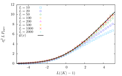
a universal scaling function, as it is independent of the underlying distribution of $K$ (number of offsprings per element). This is valid for large system sizes $L$ and small distances to the critical point, keeping $L(\langle K\rangle-1)=y$ finite. Notice that this corresponds to the usual finite-size scaling form, Eq. (1), at zero field, $h=0$, with exponents

$$\beta=\nu=1$$

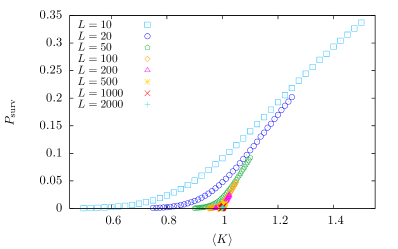
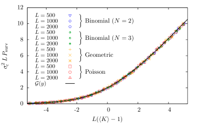
(and metric factor $b=1$). The only peculiarity is the appearance of an additional metric factor given by $\sigma_{\mathrm{c}}^{2}$. The validity of the finite-size scaling law and its universality is confronted with computer simulations of diverse branching processes in Figs. 1 and 2, with positive results.

From the finite-size scaling law, it is remarkable that keeping fixed the rescaled distance to the critical point, $y$, the survival probability decays to zero with $L$ as a power law, hyperbolically, see Eq. (4). In contrast, when the absolute distance to the critical point, $\langle K\rangle-1$, is fixed, the decay is exponential towards the infinite-size probability, $P_{\mathrm{surv}}(L)=1-q+[f^{\prime}(q)]^{L}$, see Refs. (Harris_original, , p. 16) and (Athreya, , p. 38), or Eq. (2) also.

(a)  

(b)  

Figure 1: Validity of the finite-size scaling law for the geometric Galton-Watson process. 1(a) Simulation results for the probability of surviving as a function of the mean number of offsprings $\langle K\rangle$ in a Galton-Watson process defined by a geometric distribution of $K$, given by Prob$[K=k]=p(1-p)^{k}$, for $k=0,1,\dots$ Different values of $L$ show the dependence with system size. Probabilities are estimated from 1000 independent realizations. 1(b) Same probabilities as a function of $\langle K\rangle-1$ under rescaling with $L$ and $\sigma_{\mathrm{c}}$. The collapse of the curves onto a unique scaling function, given by our theoretical result, is the signature of the validity of the finite-size scaling for large system sizes $L$ and close to the critical point $\langle K\rangle=1$.

Interesting information comes from the different limit behaviors of the scaling function,

$$\mathcal{G}(y)\rightarrow\left\{\begin{array}[]{rl}-2ye^{y}&\mbox{when }y\rightarrow-\infty,\\ 2&\mbox{when }y\rightarrow 0,\\ 2y&\mbox{when }y\rightarrow\infty,\\ \end{array}\right.$$

which yields,

$$P_{\mathrm{surv}}(L)\rightarrow\left\{\begin{array}[]{ll}2\sigma_{\mathrm{c}}^{-2}(1-\langle K\rangle)e^{-L(1-\langle K\rangle)}&\mbox{for }\langle K\rangle<1,\\ 2\sigma_{\mathrm{c}}^{-2}L^{-1}&\mbox{for }\langle K\rangle=1,\\ 2(\langle K\rangle-1)/\sigma_{\mathrm{c}}^{2}&\mbox{for }\langle K\rangle>1.\\ \end{array}\right.$$

The subcritical and supercritical results have to be understood as holding close to the critical point but for an infinitely large system.

Figure 2: Universality of the finite-size scaling. Extension of Fig. 1(b) to other Galton-Watson processes with different distributions for the number of offsprings $K$. In addition to the geometric case, the binomial distribution, with Prob$[K=k]=N!p^{k}(1-p)^{N-k}/(k!(N-k)!)$ and $N=2$ or $3$, and the Poisson distribution, with Prob$[K=k]=e^{-\lambda}\lambda^{k}/k!$, are simulated for different $\langle K\rangle$ and different system sizes $L$. The collapse of all rescaled curves validates the universality of the scaling exponents and of our scaling function.

IV Discussion

We can particularize the finite-size scaling law, Eq. (4), to the case where the number of offsprings $K$ of each element is given by a binomial distribution, defined by $N$ trials with probability of success $p$ in each trial. This distribution is relevant for the analogy with percolation Christensen_Moloney . The mean and variance are given by $\langle K\rangle=Np$ and $\sigma^{2}=Np(1-p)$. The critical point arises then at $p_{c}=1/N$ and $\sigma_{\mathrm{c}}^{2}=1-1/N$, and the finite-size scaling can be written as

$$P_{\mathrm{surv}}(L)=\frac{1}{L(1-1/N)}\mathcal{G}\left(NL\left(p-\frac{1}{N}\right)\right),$$

where the universality of Eq. (4) becomes “diffused” due to the appearance of two non-universal metric factors multiplying $L$. But it is worth mentioning that $P_{\mathrm{surv}}$ is not the order parameter defined usually in percolation, see for instance Ref. Botet .

As another illustration, if we considered a geometric distribution for $K$ (defined for $K\geq 0$), with success parameter $p$, the mean and variance are $\langle K\rangle=(1-p)/p$ and $\sigma^{2}=(1-p)/p^{2}$. The critical point is then $p_{c}=1/2$, $\sigma_{\mathrm{c}}^{2}=2$ and then the finite-size scaling transforms into

$$P_{\mathrm{surv}}(L)=\frac{1}{2L}\mathcal{G}\left(-4L\left(p-\frac{1}{2}\right)\right).$$

Notice that in this case the parameter $p$ has a different interpretation as for the binomial distribution. In any case, Fig. 2 demonstrates that the same universal finite-size scaling holds for the binomial, the geometric, and the Poisson distributions.

Summarizing, we have found that the second-order phase transition from sure extinction to non-sure extinction in the Galton-Watson branching process fulfills a finite-size scaling law, where the scaling function and the scaling exponents can be exactly derived. If the variance of the distribution of the number of offsprings per element is taken into account in the scaling law, this becomes universal, with universal metric factor, in the sense that it is exactly the same for all Galton-Watson branching processes.

References

- [1] T. E. Harris. The Theory of Branching Processes. Springer, Berlin, 1963.
- [2] K. B. Athreya and P. E. Ney. Branching Processes. Springer-Verlag, Berlin, 1972.
- [3] D. G. Kendall. The genealogy of genealogy branching processes before (and after) 1873. Bull. London Math. Soc., 7:225–253, 1975.
- [4] M. Kimmel and D. E. Axelrod. Branching Processes in Biology. Springer-Verlag, New York, 2002.
- [5] I. Pázsit and L. Pál. Neutron Fluctuations. Elsevier, Oxford, 2008.
- [6] D. Vere-Jones. A branching model for crack propagation. Pure Appl. Geophys., 114:711–725, 1976.
- [7] A. Helmstetter and D. Sornette. Subcritical and supercritical regimes in epidemic models of earthquake aftershocks. J. Geophys. Res., 107 B:2237, 2002.
- [8] K. Christensen and N. R. Moloney. Complexity and Criticality. Imperial College Press, London, 2005.
- [9] S. Zapperi, K. B. Lauritsen, and H. E. Stanley. Self-organized branching processes: Mean-field theory for avalanches. Phys. Rev. Lett., 75:4071–4074, 1995.
- [10] S. Hergarten. Branching with local probability as a paradigm of self-organized criticality. Phys. Rev. Lett., 109:–, 2012.
- [11] H. E. Stanley. Introduction to Phase Transitions and Critical Phenomena. Oxford University Press, Oxford, 1973.
- [12] J. M. Yeomans. Statistical Mechanics of Phase Transitions. Oxford University Press, New York, 1992.
- [13] H. J. Jensen. Self-Organized Criticality. Cambridge University Press, Cambridge, 1998.
- [14] G. Pruessner. Self-Organised Criticality: Theory, Models and Characterisation. Cambridge University Press, Cambridge, 2012.
- [15] A. Corral and F. Font-Clos. Criticality and self-organization in branching processes: application to natural hazards. In M. Aschwanden, editor, Self-Organized Criticality Systems, pages 183–228, 2013.
- [16] V. Privman. Finite-size scaling theory. In V. Privman, editor, Finite Size Scaling and Numerical Simulation of Statistical Systems, pages 1–98. World Scientific, Singapore, 1990.
- [17] H. E. Stanley. Scaling, universality, and renormalization: Three pillars of modern critical phenomena. Rev. Mod. Phys., 71:S358–S366, 1999.
- [18] R. Botet and M. Ploszajczak. Exact order-parameter distribution for critical mean-field percolation and critical aggregation. Phys. Rev. Lett., 95:185702, 2005.