22email: jake.stroud@wadh.ox.ac.uk 33institutetext: Mauricio Barahona 44institutetext: Department of Mathematics, Imperial College London, London, UK,
44email: m.barahona@imperial.ac.uk 55institutetext: Tiago Pereira 66institutetext: Department of Mathematics, Imperial College London, London, UK,
London Mathematical Laboratory, London, UK
66email: tiago.pereira@imperial.ac.uk
Dynamics of Cluster Synchronisation in Modular Networks: Implications for Structural and Functional Networks
1 Introduction
When using methods from network science to study real-world complex systems, one is faced with the choice of constructing either a structural or functional network that describes the relationship between the interacting components of the system. Sometimes it is more achievable or desirable to measure the dynamics of components and posit that if two components display similar activity, they are in some way dynamically linked. This gives rise to data-driven functional networks bassett . Conversely, in other situations, we may have access to structural networks representing known physical links between components. The focus of much research in complex network theory is towards gaining a greater understanding of how functional and structural networks relate to each other sporns1 .
To this end, much analysis has been conducted into network architecture and organisation. Recent results have shown that both functional and structural network representations of real world systems typically display a modular architecture bassett2 ; bullmore ; social ; soc ; cat ; maur ; Fortunato2010 . A network with a modular organization could be described as a network consisting predominantly of highly connected sub-graphs which have comparatively fewer connections to nodes outside the module. We are particularly interested in how functional modules relate to the structural modules of a network.
Synchronisation is a typical paradigm of dynamical network function. Such group collective behaviour appears with ubiquity in nature. Human hearts beat rhythmically because thousands of cells synchronise their activity cells , and the collective behaviour of neurons in the brain has been shown to be linked to Parkinson’s disease park and epileptic seizures ep . However, synchronisation does not have to be global, and can occur in particular subgroups or modules.
Over recent decades, synchronisation analysis has benefited from methods in the fields of graph theory and dynamical systems, and theories for global synchronisation have been established in terms of the network structure msf ; Heagy1995 ; Barahona2002 ; Arenas2008a . Of particular interest is the stability of the synchronised state. If global synchronisation can be maintained, this amounts to a coherent state, while if the synchronised state becomes unstable it can serve to predict a transition in the organisation of the complex system synchbar ; Belykh2004 ; Wu2005 ; August2011 ; msf ; OClery2013 .
In this chapter, we will study cluster synchronisation within modular networks of diffusively coupled oscillators. We predict the onset of stable and unstable module synchronisation by obtaining stability conditions within a densely connected module. Our model is based on the following assumptions: {svgraybox}
-
The network has a modular structure such that nodes in one module have few connections to nodes outside the module.
-
Within modules, nodes have a high mean degree and share many common neighbours.
Under these assumptions, we can perform a stability analysis independently for each module, thereby avoiding a spectral decomposition of the network adjacency matrix which poses a significant challenge for large networks. Typically, we would have to analyse as many equations as the number of nodes in a module, but because nodes within modules have a large number of common neighbours, we are able to reduce the analysis to a single equation describing the synchronisation of each module by bounding the dynamics of the external modules. Hence our analysis allows us to tackle the stability of each module independently, yet taking into account their influence on each other.
From our study of the local stability of synchronisation, we establish conditions for the persistence of stability under non-linear and linear perturbations. The stability of module synchronisation is determined as a function of: the module mean degree and matching index (defined in Section 2.2), and the isolated dynamics and coupling function. This analysis allows us to predict the formation and disintegration of functional modules depending upon the nature of the diffusive coupling between the components of the network.
Our results reveal that: {svgraybox}
-
The mean degree of the module dictates the onset of synchronisation.
-
Functional modules may not reflect fully the structural modules of a network.
As a consequence, the functional representation of a network can sometimes drastically differ from the underlying topological structure. Through the use of simulations we validate our analytical results and conclude with a discussion on how the functional network representation of a modular network relates to the underlying topological structure. The remainder of this chapter is organised as follows. Our model assumptions are formalised in Section 2. Both our analytical and numerical results are presented in Section 3. The derivation of our analytical results is then presented in Section 4. Finally we provide a conclusion and discussion in Section 5.
2 The Model
In this section we formalise our model setup. Initially we formalise some basic graph definitions we make use of as well as describing the network class we intend to study. We then present the dynamical model describing the interaction between the components of the network. See Section 2.1 for remarks regarding notation we adopt throughout the chapter.
2.1 Notation
The Jacobian matrix of a function at the point is denoted by .
When discussing synchronisation in this chapter, we imply a -synchronisation; that is, given two trajectories and we say that they are -synchronised if the difference in their state vectors are within a neighbourhood of radius at all large times
The small parameter measures the quality of synchronisation, and depends on both the isolated dynamics and coupling function as well as the network structure. This is particularly evident in the numerical simulations. To simplify the notation, we will omit the symbol when discussing -synchronisation.
We use the small ‘’ and big ‘’ notation to describe asymptotic behaviour. We write if goes to zero as tends to infinity, and we write if is bounded by a positive constant as tends to infinity.
2.2 Graphs: Basic Definitions
A graph is a set of nodes (or vertices) connected by a set of edges. Here, we will only consider simple, unweighted and undirected graphs; that is, graphs with no loops and where there is no order associated with the two vertices of each edge. We will also use the words ‘graph’ and ‘network’ interchangeably although a network commonly denotes a graph structure where some form of dynamics takes place on the nodes.
The adjacency matrix encodes the topology of the graph, with if and are connected and otherwise. Clearly, for undirected graphs. The degree of node is the number of connections it receives, that is
The mean degree for a set of nodes with cardinality is then:
We now define the matching index of a graph cat , which will play an important part in our analysis. The neighbourhood of node is the set of nodes it shares an edge with: . Clearly, for simple graphs . The matching index of nodes and is the overlap of their neighbourhoods:
The normalised matching index is then:
| (1) |
It follows that if and only if and are connected to exactly the same nodes, i.e., ; whereas if nodes and have no common neighbours cat . The mean matching index for a set of nodes with is then:
Figure 1 shows graphs with different mean degrees and matching indices.

2.3 The Modular Network
A subgraph of a graph is a set of nodes and edges of that connect any two nodes in . A structural module (or cluster) is rather loosely defined as a highly connected sub-graph with comparatively fewer connections to nodes outside the module Fortunato2010 . Conversely, by taking a dynamical perspective, popularised within the community detection literature, a module (or community) corresponds to a set of nodes and edges were a random walker is likely to become transiently trapped for a longer period of time than that expected at random zhou ; Delvenne2010 ; Schaub2012 ; maur . A prototypical example of a module would be a complete graph (or clique), where every node is connected to every other node, which is only weakly connected to other nodes. Figure 2 provides an example of such a modular network.
To make this notion more precise, we consider the mismatch index between a pair of nodes and , which corresponds to the complement of the matching index defined in Eq. (1):
| (2) |
While the matching index counts all nodes that and share, the mismatch index counts all nodes that and do not share. Hence the normalised mismatch index is:
Clearly if nodes and share exactly the same neighbours (as well as potentially being linked themselves), and if nodes and share no common neighbours.
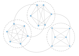
The theory we present in this chapter holds for all modules of a network G such that
| (3) |
along with the homogeneity condition
| (4) |
This final relation also implies that
Therefore from our first relation (Eq. (3)), a module will have a high matching index, that is, nodes within a module will have a large number of common neighbours. Our second relation (Eq. (4)), allows us to approximate the degree of each node in by the module mean degree and, certainly for small networks, excludes the possibility of any hubs (highly connected nodes) occurring in a module. As a consequence, module can be described by the number of nodes it contains and its mean degree: .
We note that the matching index does not distinguish between a lack of common neighbours within the module and additional (unshared) links to nodes outside the module. Therefore, a high matching index not only guarantees that nodes within a module share similar neighbours but that they also have a comparatively low number of links to nodes outside the module. In clustsynch , the edges of a graph were decomposed into inter-module and intra-module edges. They showed that this classification of edges distinguishes the formation of functional modules.
2.4 The Dynamical Model: Network of Diffusively-Coupled Bounded Systems
We now introduce some dynamics on each node of the graph. The dynamics of each node is governed by -dimensional dynamics:
| (5) |
where is a smooth vector field, and we also assume that the solutions of this isolated system are bounded, i.e., for all there exists a such that . The boundedness of the dynamics of the nodes encompasses a wide variety of stationary and oscillatory (periodic and chaotic) systems evo .
The influence that neighbour exerts on the dynamics of node is assumed to depend on the difference of their state vectors: . This type of coupling tries to equalise all states of the nodes and it is in this sense that it is called a diffusive coupling. The model accounts for the influence of all neighbours in a network with adjacency matrix , which is assumed to be given. The dynamics of node in a network of diffusively coupled elements is then given by:
| (6) |
where is the overall coupling strength and is the coupling function. Hence the coupling between elements is given in terms of the adjacency matrix and modulates the influence between connected nodes. Note that we assume identical elements, i.e., in our model, the dynamics and coupling are identical for all nodes.
3 Results
In this section, we first state briefly our main analytical results, which are derived in detail in Section 4. We then provide extensive numerical simulations to illustrate our findings.
3.1 Summary of Analytical Results
Firstly, we state our assumptions regarding the dynamics of the system.
-
A1
: The coupled node dynamics in Eq. (6) are bounded: there is a constant such that
-
A2
: The variational equation
(7) where is the trajectory of any node, admits a uniformly asymptotic trivial solution for , where the both the upper and lower bounds depend on the dynamics and coupling functions: and 111 We see the equation as a parametric equation in the same spirit as the master stability function approach Barahona2002 ; pec ; PRL_2013 , hence we omit the subindex that explicitly shows the dependence on the node. . That is, the solution of the variational equation is a contraction:
with
where uniformly and .
Assumption A1 is natural in applications. In particular, if a Lyapunov function exists for the isolated dynamics (5) with an absorbing domain, it is possible to show that the network solution satisfies A1 tiago . Assumption A2 is similar to the master stability function approach pec . The main difference is that in the master stability function, the trajectory corresponds to the a modified (perturbed) solution of the uncoupled dynamics, whereas here it corresponds to the trajectory of a coupled node. Depending on the structure of the coupling function this difference is immaterial Nonlinearity . Our numerical analysis shows that the values of and from the master stability function provide a good approximation.
Remark 1
If the coupling function is a positive definite matrix, then the results of Ref. Nonlinearity demonstrate that and . Moreover, the contraction exponent is given by
where is the smallest eigenvalue of .
Using these two assumptions in combination with the modular structure of the network, we derive, in Section 4, a stability condition for the synchronisation of modules which does not require a spectral analysis of the network adjacency matrix. This is a consequence of the high matching index within modules. Our results enable the prediction of functional module formation and disintegration depending on the structural properties of the module and the dynamical properties of the nodes.
Our main finding is the following: {svgraybox} Consider the modular network containing a module with nodes and mean degree . Assume that A1 and A2 hold, such that the system in Eq. 7 is a contraction for . If the matching index of the module is high, then the critical coupling strengths for synchronisation and for desynchronisation are given by
| (8) |
where . Hence, for , such that , the nodes in exhibit stable synchronised dynamics
| (9) |
This result shows that, under these assumptions, the average degree of the module has an effect on the coupling interval that guarantees synchronisation in the module: only if the coupling is such that the functional and structural modules coincide. If the coupling strength is too large () or too small (), the functional module disintegrates and no longer reflects the structural module. We call this change the bifurcation between functional and structural modules. Importantly, the intervals in which synchronisation is stable will be different for different modules, depending on their mean degree.
Remark 2
If the coupling function is a positive definite matrix, then . Therefore for this class of coupling function and large enough values of the coupling , the functional modules mirror all the structural modules in the network. On the other hand, if no functional modules will be apparent. In between those two limits, only some of the structural modules will be reflected as functional modules. This is the case of the coupling .
Note also that the solutions under cluster synchronisation may not be similar to the solutions of the invariant synchronisation manifold of the whole network
Therefore the dynamics of nodes in different modules can be very different to each other and, in particular, to the global synchronous dynamics of the network. In our analysis, we effectively decompose a modular network into individual modules with low inter-module connectivity and predict the onset of stable synchronisation based upon the mean degree within a module. For the derivation of our analytical results, see Section 4.
3.2 Numerical Simulations
To illustrate our analytical results we consider numerical simulations of the paradigmatic example of a network of diffusively coupled identical Rössler oscillators. The isolated dynamics of each oscillator is described by the system of differential equations
with the standard parameter values and . For these values, we know the system exhibits a chaotic attractor and that all trajectories eventually enter a compact set, thereby satisfying our assumptions regarding from Section 2.4.
For a network of diffusively coupled Rössler oscillators, the dynamics of a node are governed by the diffusive model (Eq.(6)), repeated here for clarity
| (10) |
where is the global coupling strength, is the inner coupling matrix, and encodes the graph topology.
To numerically determine the stability of synchronisation for a system of coupled oscillators, we construct a correlation matrix for a particular coupling strength . This correlation matrix describes the pairwise similarity between the dynamics of all oscillators in the system averaged over some large time
where the elements of the matrix are defined as:
for nodes and and
Using this notation, we also define the mean correlation between the dynamics of a set of nodes
We integrated Eq. (10) using an Adams-Bashforth multi-step scheme together with an intial fourth order Runge-Kutta algorithm using a step size of 0.001. The initial states of the oscillators were randomised between and .
We calculated the correlation matrix for a network with a modular structure, varying coupling strengths and for two coupling schemes: and , where
The case corresponds to each variable and being coupled to the same variable of all its neighbours, while corresponds to only the variable being coupled to its neighbouring nodes.
Dynamics within a modular network
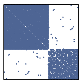
We first present the numerical results of the simulations of the modular network shown in Fig. 3. The network has two modules and generated according to an Erdös-Rényi architecture: contains nodes with and ; contains nodes with and . The inter-module connections are low compared with the intra-module links, as implied by the high module matching indices. In these simulations, we use the -coupling: . The results of the functional analysis are presented in Figure 9.
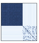

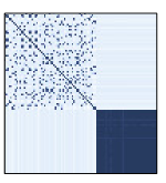
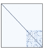
 \samenumber
Figures 9 to 9 display heat map representations of the correlation matrix for increasing coupling strengths . Darker regions correspond to higher correlation between node dynamics. From the analysis of the master stability function of the Rössler system with these parameters and -coupling, it has been found that the region of stable synchronisation are bounded by and msf . We can then use these numbers to approximate the regions of stable synchronisation for modules and : and for ; whereas and for . These regions are indicated by the illustration inset in Figure 9.
Our numerics show that when there is no correlation between the dynamics of the nodes. This is expected since there is no interaction between the oscillators. For , has synchronised and some nodes in are beginning to show cohesive dynamics. This is expected since the coupling strength has entered the predicted stable synchronisation region for but not for . For , both modules have synchronised, but the dynamics of the two modules are uncorrelated as indicated by the pale off-diagonal regions. This is a result of the low inter-module connectivity222Under certain conditions, it is possible for two modules to synchronise and this is explored elsewhere such as clustersynch .. For (Figure 9), module has already desynchronised, while remains synchronised. As the coupling strength is increased further, also desynchronises.
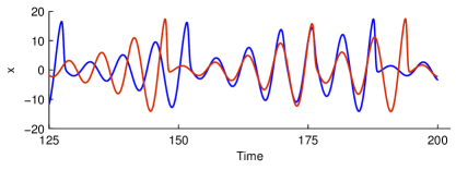
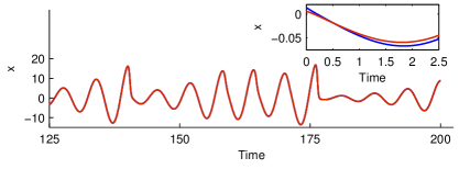
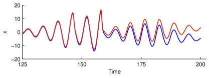
The dynamical behaviour of the clusters is perhaps expressed more clearly when analysing the time evolution of the oscillators. Figure 13 displays the evolution of the variable of two oscillators in module for increasing coupling strengths. In Figure 12, where , we observe, as expected, that the dynamics of the two oscillators are uncorrelated. For in Figure 12, the two oscillators synchronise. The inset in this figure demonstrates that the two oscillators have differing but close initial conditions and due to the coupling strength, soon achieve stable synchronisation. Finally, for (Figure 12), the oscillators initially synchronise before diverging after a short time and then remain uncorrelated thereafter.
Relation between the critical coupling strength and the module mean degree
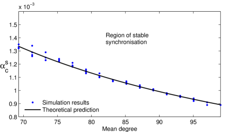
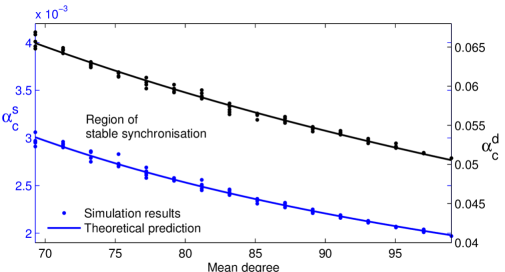
We now examine how the critical coupling strength required for stable synchronisation within a module depends upon its mean degree. To this end we simulated a network of nodes for varying matching indices between and which will act as a paradigmatic example of a module with no inter-module links, thereby removing any external perturbations from other modules. We then determined the coupling strength such that for both and . We repeated simulations times for varying network adjacency matrices.
Along with the simulations, we indicate the predicted critical coupling strength which depends inversely upon the mean degree of the module as determined by our methodology. We demonstrate this by fitting the simulation results to an expression of the form
| (11) |
where and are fitting parameters.
Remark 3
The precise bounds for the critical coupling strength depends on the actual node degrees and not only the mean degree (see the derivation of the results in Section 4 for details). However, since node degrees are close to the mean degree we can approximate , where is treated as a free parameter. The parameter effectively allows for inhomogeneities within the module structure to produce a small perturbation to the critical coupling strength required for stable synchronisation, details on these perturbations can be found in Section 4.4.
Figure 14 displays the results when coupling all components of the dynamics with . As expected, all nodes in the module will synchronise given a strong enough coupling strength and the module will remain synchronised as the coupling strength is increased thereafter. The simulations follow an inverse dependence upon the mean degree of the module (Eq. (11)), as expected from our results.
Figure 15 displays the results when coupling only the component of the dynamics, corresponding to . We see that for a module with a high matching index, all nodes will synchronise above a coupling strength and will then desynchronise as the coupling strength is increased further. Again, from the fitted curves, the critical coupling strengths required for synchronisation and desynchronisation display an inverse dependence upon the module mean degree in line with our results.
Remark 4
When setting in the curve fitting (corresponding to perfectly homogeneous node degrees), we can directly compare our results with those obtained in the literature from analysing the master stability function, which have shown and for this system msf . From our fits, allowing for a stable synchronisation region to be given by , we obtain and in close agreement with the master stability function bounds, as expected from our analytical results.
4 Derivation of our Analytical Results
Before detailing the derivation of our results below, we briefly outline our strategy. Starting from Eq. (6), we define
| (12) |
where is a module, and analyse the dynamics of . To this end, we take the following four steps.
-
1.
First, for sufficiently small, we obtain the linearised equation for :
(13) where and are to be determined and depend on both the node dynamics and network structure. By Taylor’s Theorem, the remainder is and it can be dealt with in step 2.
-
2.
We then analyse the associated homogeneous equation
and, by Eq. (7), represent in terms of its associated evolution operator
Our assumption A2 guarantees that the trivial solution of the above equation is uniformly asymptotically stable, that is, for some ,
-
3.
We then solve Eq. (13) using the method of variation of parameters
and by defining , from the triangle inequality we obtain
- 4.
We now explain these steps in more detail.
4.1 Obtaining the Variational Equation
For some such that is sufficiently small, we can expand as a Taylor series, and after some manipulations we obtain
where is the degree of node as given in Section 2.2. Without loss of generality, we assume and set to obtain
| (14) |
where
| (15) |
and
| (16) |
This is the first variational equation. Note, we truncated our Taylor expansion in up to first order and by Taylor’s Theorem we know the remainder satisfies .
4.2 The Homogeneous Equation
We now consider the homogeneous part of Eq. (14)
| (17) |
Notice the rescaling brings the above equation (Eq. (17)) to Eq. (7). Therefore, if
Eq. (17) has an evolution operator satisfying
| (18) |
Now, since modules will have a large number connections and nodes will share many common neighbours, will be close to the mean degree (see our network assumptions Eq. (3) and Eq. (4)). This means that in leading order in , the stability condition is given by
where takes into account the fluctuation between and the mean degree . After some rearrangements we obtain
| (19) |
Then for large we see that Eq. (19) resembles Eq. (8). Furthermore, according to Remark 1, if is positive definite, we obtain and
| (20) |
Then for satisfying in Eq. (20), we obtain a uniform contraction. It remains to show that the perturbations will not destroy the synchronisation property.
4.3 The Perturbed Equation
4.4 Bounds for the Perturbation
We give the argument for Eq. (21). The argument for Eq. (22) is similar. We first recall the mismatch index Eq. (2):
Then since since the trajectories are bounded and the coupling function is smooth, we can bound
for a positive constant , and since
from Eq. (16), we obtain
| (23) |
Then, motivated by the matching index notation in Eq. 1, we can introduce
to obtain
| (24) |
Therefore, for the perturbation to be small, we require:
-
•
The difference in node degrees within a module to be low.
-
•
Nodes to share many common neighbours within a module.
-
•
Nodes to have comparatively fewer connections to nodes outside the module.
The final two requirements emerge via the matching index in Eq. (24) since penalises for not only a lack of shared nodes within a module but also for additional (unshared) connections to nodes outside the module. Then, from our network assumptions (Eq. (3) and Eq. (4)) along with statisfying the stability condition Eq. (19), by Eq. (21) and Eq. (23), we obtain
Therefore the stability of module synchronisation depends upon the module mean degree and the extent to which synchronisation can be achieved depends upon the matching index within a module. These conditions will clearly vary between modules and our conditions only guarantee individual modules to synchronise independently as opposed to global network synchronisation.
5 Conclusion and Discussion
We have shown that the stability of module synchronisation in complex modular networks can be predicted based upon the module mean degree given certain assumptions on the component dynamics and network structure. Our key assumption on the modular structure is that nodes within modules share many common neighbours and inter-module connections are weak in comparison.
Our analysis revealed two basic scenarios for module synchronisation. If the coupling function is linear and positive definite, we showed that the functional modules reflect the structural modules. In this case, as the coupling strength is increased, the module with the largest mean degree synchronizes first, then more and more modules achieve synchronisation. In this case, the dynamics of the network mirror the structural properties of the network.
However, for more general couplings, typically our stability criterion A2 is satisfied, see Ref. msf . In this case, we observe interesting dynamical behaviour as the coupling parameter is increased where, in a first stage, modules of synchronised nodes can form and reflect the structural organization, but for large couplings the synchronisation becomes unstable and functional modules disintegrate. This scenario corresponds to bifurcations between the functional and structural properties.
Our assumptions on the structure of the modules allowed for an analytical treatment of these scenarios and enabled us to determine the critical coupling strengths for synchronisation and desynchronisation. Additionally, we showed that the module matching index dictates the quality of synchronisation. Moreover, our present approach can be used to explain the synchronised dynamics of groups of nodes not necessarily forming modules such as hub synchronization Murilo ; HubPRE , since their matching index may be high and the degrees similar.
These results can be of importance for functional network analysis and enhance our understanding of the relation between the functional and structural network. Indeed, even though a module may possess the structural properties required for synchronisation, the functional modules may not reflect the structural modules of a network.
References
- (1) D.S. Bassett, M. Lynall, Network Methods to Characterize Brain Structure and Function, Cognitive Neurosciences: The Biology of the Mind (Fifth Edition).
- (2) C.J. Honey, O. Sporns, L. Cammoun, X. Gigandet, J.P. Thiran, R. Meuli, P. Hagmann, Predicting human resting-state functional connectivity from structural connectivity, Proc Natl Acad Sci USA 106: 2035-40, 2009
- (3) D.S. Bassett, N.F. Wymbs, M.A. Porter, P.J. Mucha, J.M. Carlson, S.T. Grafton, Dynamic reconfiguration of human brain networks during learning, PNAS 108, 7641 (2011).
- (4) D. Meunier, R. Lambiotte, E.T. Bullmore, Modular and hierarchically modular organisation of brain networks Front. Neurosci. 4, 200 (2010).
- (5) N. Mishra, R. Schreiber, I. Stanton, R.E. Tarjan, Clustering Social Networks, Algorithms and Models for the Web-Graph, Springer (2007).
- (6) S. Wang, C. Zhou, Hierarchical modular structure enhances the robustness of self-organized criticality in neural networks, New Journal of Physics 14, 023005 (2012)
- (7) G. Zamora-Lopez, C. Zhou, J. Kurths, Cortical hubs form a module for multisensory integration on top of the hierarchy of cortical networks, Font. Neuroinform. 4, 1 (2010).
- (8) S. Strogatz, Synch: The Emerging Science of Spontaneous Order, Hyperion, New York (2003).
- (9) P. Tass, M.G. Rosenblum, J.Weule, J. Kurths, A. Pikovsky, J. Volkmann, A. Schnitzler, H.J. Freud, Phys.Rev.Lett. 81, 3291, 1998
- (10) J. Milton, P. Jung (Ed), Epilepsy as a Dynamic Disease, Springer (2010).
- (11) L.M. Pecora, M. Barahona, Synchronisation of Oscillators in Complex Networks, Chaos and Complexity Letters 1, 61 (2005).
- (12) H. Zhou, Network landscape from a Brownian particle’s perspective, Phy. Rev Phys. Rev. E 67, 041908 (2003).
- (13) J-C. Delvenne, M.T. Schaub, S.N. Yaliraki, M. Barahona, The stability of a graph partition: A dynamics-based framework for community detection, Springer (2013).
- (14) W. Lu, B. Liu, T. Chen, Cluster synchronisation in networks of coupled non-identical dynamical systems, Chaos 20, 013120 (2010).
- (15) T. Pereira, Stability of Synchronized motion in complex networks, arXiv:1112.2297 (2012).
- (16) L.M. Pecora, T.L. Carrol, Master Stability Functions for Synchronized Coupled Systems, Phys. Rev. Lett. 80, 2109, 1998
- (17) T. Pereira, J. Eldering, M. Rasmussen, A. Veneziani, Towards a theory for diffusive coupling functions allowing persistent synchronization, Nonlinearity 27, 501, 2014
- (18) T. Pereira, D. Eroglu, G. Bagci, U. Tirnakli, and H.J. Jensen, Connectivity-Driven Coherence in Complex Networks, Phys. Rev. Lett. 110, 234103 (2013)
- (19) L. Huang, Q. Chen, Y-C. Lai, L. Pecora, Generic behaviour of master-stability functions in coupled nonlinear dynamical systems, Physical Review E, 80, 036204 (2009).
- (20) W. Jian-She, J. Li-Cheng, C. Guan-Rong, Cluster Synchronisation in a network of non-identical dynamic systems, Chin. Phys. B 20, 060503 (2011).
- (21) M.S. Batista, et al., Collective Almost Synchronisation in Complex Networks, PLoS ONE 7(11): e48118 (2012).
- (22) T. Pereira, Hub Synchronization in Scale Free Networks Phys. Rev. E 82, 036201 (2010).
- (23) S. Fortunato, Community detection in graphs, Physics Reports 486(3-5), 75 (2010).
- (24) J.F. Heagy, L.M. Pecora, T.L. Carroll, Short-Wavelength bifurcation and size instabilities in coupled oscillator-systems, Physical review letters 74(21), 4185 (1995).
- (25) M. Barahona, L.M. Pecora, Synchronization in Small-World Systems, Phys. Rev. Lett. 89, 054101 (2002).
- (26) A. Arenas, A. Díaz-Guilera, J. Kurths, Y. Moreno, C. Zhou, Synchronization in complex networks, Physics Reports 469(3), 93 (2008).
- (27) V.N. Belykh, I.V. Belykh, M. Hasler, Connection graph stability method for synchronized coupled chaotic systems, Physica D: nonlinear phenomena 195(1), 159 (2004).
- (28) C.W. Wu, Synchronization in networks of nonlinear dynamical systems coupled via a directed graph, Nonlinearity 18(3), 1057 (2005).
- (29) E. August, M. Barahona, Obtaining certificates for complete synchronisation of coupled oscillators, Physica D: Nonlinear Phenomena 240(8), 795 (2011).
- (30) N. O’Clery, Y. Yuan, G.B. Stan, M. Barahona, Observability and coarse-graining of consensus dynamics through the External Equitable Partition, Physical Review E 88(4), 042805 (2013).
- (31) J.C. Delvenne, S.N. Yaliraki, M. Barahona, Stability of graph communities across time scales, Proceedings of the National Academy of Sciences 107(29), 12755 (2010).
- (32) M.T. Schaub, J.C. Delvenne, S.N. Yaliraki, M. Barahona, Markov dynamics as a zooming lens for multiscale community detection: non clique-like communities and the field-of-view limit, PLoS ONE 7(2), e32210 (2012).
- (33) G. Teschl, Ordinary differential equations and Dynamical Systems, Volume 140, Amer. Math. Soc., Providence, 2012