Intrinsic alignments of SDSS-III BOSS LOWZ sample galaxies
Abstract
Intrinsic alignments (IA) of galaxies, i.e. correlations of galaxy shapes with each other (II) or with the density field (gI), are potentially a major astrophysical source of contamination for weak lensing surveys. We present the results of IA measurements of galaxies on –Mpc scales using the SDSS-III BOSS LOWZ sample, in the redshift range . We extend the existing IA measurements for spectroscopic LRGs to lower luminosities, and show that the luminosity dependence of large-scale IA can be well-described by a power law. Within the limited redshift and color range of our sample, we observe no significant redshift or color dependence of IA. We measure the halo mass of galaxies using galaxy-galaxy lensing, and show that the mass dependence of large-scale IA is also well described by a power law. We detect variations in the scale dependence of IA with mass and luminosity, which underscores the need to use flexible templates in order to remove the IA signal. We also study the environment dependence of IA by splitting the sample into field and group galaxies, which are further split into satellite and central galaxies. We show that group central galaxies are aligned with their halos at small scales and also are aligned with the tidal fields out to large scales. We also detect the radial alignments of satellite galaxies within groups. These results can be used to construct better intrinsic alignment models for removal of this contaminant to the weak lensing signal.
keywords:
galaxies: evolution – cosmology: observations –large-scale structure of Universe –gravitational lensing: weak1 Introduction
The deflection of light rays due to the gravitational effects of matter, gravitational lensing, changes both the observed shape and size of distant galaxies. Weak lensing, the statistical study of such tiny shape distortions, has emerged as an important tool in cosmology to study and map the distribution of dark matter as well as to study the effects of dark energy. Due to its sensitivity to the total matter content, weak lensing is theoretically a clean probe for dark matter and dark energy, but it is affected by a number of potential systematic sources (see, e.g., Weinberg et al., 2013). Much effort has been put into controlling the observational systematics arising from the effect of the point-spread function (PSF) on the estimated galaxy shape distortions. Future surveys like LSST111http://www.lsst.org/ (LSST Science Collaboration et al., 2009), Euclid222http://sci.esa.int/euclid/, http://www.euclid-ec.org (Laureijs et al., 2011) and WFIRST-AFTA 333http://wfirst.gsfc.nasa.gov/ (Spergel et al., 2013) aim to bring these systematics below the percent level, with comparable improvement being needed on astrophysical sources of contamination to the weak lensing measurements.
Intrinsic alignments of galaxies is perhaps the most important astrophysical systematic for weak lensing (for a review see, Troxel & Ishak, 2014). It is the coherent alignments of the shapes of physically nearby galaxies which can mimic the weak lensing signal. One likely explanation for intrinsic alignments is that they are an environmental effect, whereby the local or large-scale tidal fields can shear and align the galaxy shapes, producing shape correlations. These correlations violate the assumption in weak lensing studies that observed correlations in galaxy shapes are only caused by gravitational lensing. Hirata & Seljak (2004) developed the linear alignment model for the intrinsic alignments, assuming that intrinsic alignments are set by tidal fields at the time of galaxy formation (Catelan, Kamionkowski & Blandford, 2001). This model was later extended by Bridle & King (2007) to non-linear scales using the full non-linear matter power spectrum. To extend this model inside of dark matter halos, Schneider & Bridle (2010) developed the halo model of intrinsic alignments, which assumes that satellites are aligned radially within the halo, with central galaxies (BCGs or BGGs) being preferentially aligned with the shape of the halo. There is also extensive literature on spin alignments of spiral galaxies which we will not explore in this paper (see, e.g., Crittenden et al., 2001; Capranico, Merkel & Schäfer, 2013; Zhang et al., 2015). Constraining these models observationally is important for all techniques for mitigating intrinsic alignments in future weak lensing surveys that involve marginalizing over models with some free parameters (e.g., Joachimi & Bridle, 2010); these techniques require valid models, and priors on the model parameters.
Intrinsic alignments are also interesting from the galaxy formation perspective, as the alignments of galaxies with their dark matter halos and the alignments of dark matter halos themselves are intricately related to the processes involved in galaxy formation and evolution. Many studies have concentrated on studying intrinsic alignments of dark matter halos in cosmological simulations (for example, Croft & Metzler, 2000; Hopkins, Bahcall & Bode, 2005; Basilakos et al., 2006; Heymans et al., 2006; Kang et al., 2007; Kuhlen, Diemand & Madau, 2007a; Faltenbacher et al., 2008; Knebe et al., 2008; Pereira, Bryan & Gill, 2008; Schneider, Frenk & Cole, 2012; Forero-Romero, Contreras & Padilla, 2014). These studies have found that dark matter halo shapes tend to align with each other and with the large scale structure (Schneider, Frenk & Cole, 2012; Forero-Romero, Contreras & Padilla, 2014). These alignments depend on the halo properties such as mass, radii and redshift. More massive halos in general have higher ellipticities and show stronger alignments. Ellipticities and alignments also increase with the redshift, with higher redshift halos being more elliptical and showing stronger alignments (see, for example, Hopkins, Bahcall & Bode, 2005; Ragone-Figueroa et al., 2010; Wang et al., 2011; Schneider, Frenk & Cole, 2012). This is consistent with the picture of alignments being imprinted at the time of formation which can then get disrupted by various processes such as halo mergers and hence alignments decrease with redshift. There is also radial dependence, where the ellipticity and the alignment signal varies with the radii used to measure the shapes of the halos, with outer radii being more elliptical and showing stronger alignments (see, for example, Hopkins, Bahcall & Bode, 2005; Schneider, Frenk & Cole, 2012; Tenneti et al., 2014a, b).
At small scales, the subhalos within larger halos tend to align radially within their host halos (Kuhlen, Diemand & Madau, 2007b; Knebe et al., 2008; Pereira, Bryan & Gill, 2008; Faltenbacher et al., 2008). These radial alignments primarily originate from tidal torquing of galaxies within host halo (Pereira, Bryan & Gill, 2008), are independent of host halo mass (Knebe et al., 2008; Pereira, Bryan & Gill, 2008), depend on the distance of the subhalo from the center of the host halo, and can be observed out to large distances of (Faltenbacher et al., 2008). The satellite alignment signal also has some contribution from the anisotropic satellite distribution, with satellites distributed preferentially along the host halo major axis (Faltenbacher et al., 2008).
Several studies have also looked at the relation between dark matter shapes and galaxy shapes by populating the dark matter halos with galaxies using semi analytic models (Okumura, Jing & Li, 2009; Faltenbacher et al., 2008; Schneider, Frenk & Cole, 2012; Joachimi et al., 2013a, b). For example, Joachimi et al. (2013a, b) studied shapes and intrinsic alignments of COSMOS galaxies by populating dark matter halos in the Millennium simulation (Springel et al., 2005) with galaxies using semi-analytical methods, finding a strong dependence of intrinsic alignments on scale, redshift and galaxy type. Faltenbacher et al. (2008) also compared the results from semi-analytic modeling and SDSS DR6 LRGs and found that a mean misalignment angel of degrees between the dark matter shape and galaxy shapes is necessary to explain the observations (see also Okumura, Jing & Li, 2009; Schneider, Frenk & Cole, 2012). Tenneti et al. (2014a) also studied the orientations of stellar components of galaxies within their halos using the MassiveBlack-II (MB-II) hydrodynamical simulation (Khandai et al., 2014), and found that galaxy shapes are preferentially aligned with their dark matter halos with an average misalignment angle of degrees, with the degree of misalignment being a strong function of mass.
Observationally, several studies have detected the intrinsic alignments for Luminous Red Galaxies (LRGs) to tens of Mpc scales (Mandelbaum et al., 2006; Hirata et al., 2007; Okumura, Jing & Li, 2009; Joachimi et al., 2011), finding the radial dependence of the signal to be consistent with the linear alignment model. Hirata et al. (2007) and Joachimi et al. (2011) also observed luminosity dependence of intrinsic alignments, with more luminous objects having stronger alignments. Many studies have also tried to measure intrinsic alignments within halos using large cluster samples (Sifón et al., 2014; Schneider et al., 2013; Hung & Ebeling, 2012; Hao et al., 2011), but so far, satellite alignments within groups and clusters have not been conclusively detected. Zhang et al. (2013) used the Sloan Digital Sky Survey (SDSS) DR7 data to reconstruct the cosmic tidal field, and observed that the major axis of galaxies tends to be aligned with the direction of the filament or the plane of the sheet in which they live. They also observed color, environment and luminosity dependence of this alignment, with central, red and brighter galaxies showing stronger alignments. Blazek et al. (2012) and Chisari et al. (2014) also developed methods to measure intrinsic alignments using more general photometric samples from SDSS. When using photometric redshifts, intrinsic alignments measurements suffer from contamination from weak lensing. After accounting for possible weak lensing contamination, Blazek et al. (2012) and Chisari et al. (2014) found the intrinsic alignments signals for typical galaxies to be consistent with null detection.
In this work, we will extend the study of intrinsic alignments in LRGs to more faint objects using the low redshift (LOWZ) spectroscopic sample of LRGs from the SDSS-III BOSS survey. The LOWZ sample covers the same redshift range as the LRG sample used by Hirata et al. (2007), but it extends to lower luminosities, with mean and median band magnitude fainter by magnitudes in the redshift range that we use in this work. LOWZ also has higher comoving number density , an increase by a factor of 3. We test the validity of the non-linear alignment model in both the linear and quasi-linear regimes using shape-density cross correlations for various samples defined using different galaxy properties. We study the environmental dependence of intrinsic alignments by identifying galaxies in groups and study the intrinsic alignments for satellites, BGGs (brightest group galaxies), and field galaxies (galaxies in groups of multiplicity one in our sample). We also model the small-scale signal using a halo model fitting function from Schneider & Bridle (2010), and study the variations in small-scale intrinsic alignment amplitude with different galaxy properties.
This paper is organized as follows: in section 2, we describe the linear alignment model of intrinsic alignments along with the halo model and the two point correlation functions we use to measure intrinsic alignments. Section 3 describes the SDSS-III BOSS LOWZ sample and selection criteria for the different sub-samples that we use. We present our results in section 4 and conclude in section 5.
Throughout we use standard cosmology with , , , , , (WMAP9, Hinshaw et al., 2013). All the distances are in comoving , though as mentioned above was used to calculate absolute magnitudes and to generate predictions for the matter power spectrum.
2 Formalism and Methodology
We model galaxy shapes as some purely random shape, plus two small but coherent shape distortions (“shears”), one due to intrinsic alignments (e.g., from some large-scale tidal field) and the other due to gravitational lensing. The coherent part of the shears can be written as , where is the lensing shear and is the intrinsic shear. The two point correlation function for shear thus has the following contributions:
| (1) |
is the desired lensing signal, while the contribution comes from two nearby galaxies that are affected by the same tidal field and contribution comes from the pair where one galaxy shape is affected by the tidal field of the gravitational potential it lives in while a background galaxy is lensed by the same potential, see Hirata & Seljak (2004). In Sec. 2.1 we describe the linear alignment model used to model intrinsic alignments at large scales, followed by the halo model prescription in Sec. 2.2, which describes the intrinsic alignments at small scales.
2.1 Linear alignment model
One popular formalism to study intrinsic alignments at large scales is the linear alignment model (Catelan, Kamionkowski & Blandford, 2001; Hirata & Seljak, 2004; Chisari & Dvorkin, 2013). In this section, we briefly describe the main features of the model.
The linear alignment model is based on the assumption that the intrinsic shear of galaxies is determined by the tidal field at the time of formation of the galaxy (assumed to be during matter domination; Catelan, Kamionkowski & Blandford, 2001). Thus, we can write the intrinsic shear in terms of the primordial potential as
| (2) |
Using the form of described in Eq. (2), Hirata & Seljak (2004) derived the power spectrum for the two-point matter-intrinsic alignments correlation functions, relating them to the linear matter power spectrum, .
| (3) | ||||
| (4) | ||||
| (5) |
Here, () is the cross-power spectrum between the galaxy density field and the galaxy intrinsic shear along (at 45∘ from) the line connecting a pair of galaxies; is the shape- shape power spectrum for alignment along the line joining each pair of galaxies in the two-point correlations; and is the linear galaxy bias. Following Joachimi et al. (2011), we fix , and use an arbitrary constant to measure the amplitude of intrinsic alignments for different samples. is the linear growth factor, normalized to unity at .
To measure the two-point correlation functions, we cross-correlate two samples of galaxies, with one sample used as a biased tracer of the matter density (“density sample”, denoted ) and the other sample with shapes to trace the intrinsic shear (“shape sample”, denoted ). See Sec. 2.3 for more details. The galaxy bias entering Eq. (3) is the bias of the density sample, while is measured for shape sample.
Bridle & King (2007) suggested using the full non-linear matter power spectrum, , in Eqs. (3)–(5) to extend the linear alignment model to quasi-linear scales. This model is called the non-linear linear alignment (NLA) model. While there are a number of reasons why this substitution of the non-linear matter power spectrum is unlikely to be valid to very small scales (see discussion in Bridle & King, 2007), it should allow at least some extension to smaller scales, and use of this model will permit us to compare our results more easily with many other works that have also adopted this model. In this work, we will use the non-linear matter power spectrum based on halofit model (Smith et al., 2003), generated with software CAMB (Lewis & Bridle, 2002), with fixed WMAP9 cosmology from Hinshaw et al. (2013). The expressions in Eqs. (3)–(5) can be Fourier transformed to get the 3d correlation functions:
| (6) |
Here , and is the linear redshift distortion parameter444 We do not explicitly account for the Fingers of God effect due to the virial motions of galaxies within halos. However, these are expected to be negligible in the projected correlations which are obtained by integrating along the line-of-sight between . with the Kaiser factor which accounts for the effects of redshift-space distortions (RSD, see Appendix A). For quantities that include a galaxy overdensity, the relevant is defined as , where is the logarithmic growth rate at redshift and is the galaxy bias of the sample. For the case of the shear, there is no RSD effect at leading order (, see Appendix A). In CDM, for a wide range of redshifts, . For the purpose of modelling projected correlation functions, van den Bosch et al. (2013a) show that the Kaiser approximation is sufficiently accurate.
From data, we most easily measure , the 2d (projected) correlation function, which can be obtained by integrating the 3d correlation function over the line of sight separation
| (7) |
Here is the 2d projected separation and is the redshift window function (Mandelbaum et al., 2011):
| (8) |
and are the redshift probability distributions for shape and density sample respectively and is the comoving distance to redshift .
Doing the integral in Eq. (7), we get the 2d correlation functions:
| (9) |
where is the galaxy bias for density sample, while . is expected to be zero by symmetry. The projected intrinsic alignments auto- correlation function is defined as
| (10) |
As discussed earlier, there is no RSD correction in at leading order. Thus, the RSD correction555This is different from equation C.1 in Blazek, McQuinn & Seljak (2011) and equation 12 in Chisari & Dvorkin (2013), which have an incorrect RSD factor in . in is only (from the galaxy overdensity ) and there is no RSD correction in at leading order (see Appendix A for derivation).
To measure the bias of the density sample and of the shape sample, , we measure the two-point galaxy-galaxy cross correlation function
| (11) |
Intrinsic alignments measurements that do not use spectroscopic redshifts suffer from gravitational lensing as a potential contaminant (Joachimi et al., 2011; Blazek et al., 2012; Chisari et al., 2014). Since we use spectroscopic redshifts to select galaxy pairs, we expect negligible lensing contamination in our measurements from galaxy-galaxy lensing. Hence we do not include any contamination signals in our model.
2.2 Halo model
To extend this model of intrinsic alignments into scales comparable to or smaller than the sizes of dark matter halos, Schneider & Bridle (2010) proposed the halo model for intrinsic alignments. The halo model assumes that BCGs (Brightest Cluster Galaxy) or BGGs (Brightest Group Galaxy) are at the center of dark matter halos, with their shapes aligned with the host halos. Satellite galaxies tend to align radially with the major axis pointing towards the center of the halo. In practice there can be substantial contamination in small scale intrinsic alignments signal due to off-centering of BCGs, as well as misalignments between dark matter and baryons.
Schneider & Bridle (2010) calculated the 1-halo intrinsic alignments power spectrum using Monte Carlo simulations with the aforementioned complications, and they provide a fitting function for the halo model, given by
| (12) |
The parameters are given by
| (13) |
is the redshift and are the parameters that we keep fixed to values described in Table 1. Our choice of and values are the same as in Schneider & Bridle (2010), while the are different, chosen to fit the shape of for LOWZ sample. As in Sec. 2.1, we do the Fourier transform and line-of-sight integration to get
| (14) |
When computing the correlation functions from data, we use , which is much larger than a typical halo size. The integral can then be approximated as a delta function, and Eq. (14) can be written as
| (15) |
| Parameter Index | |||
|---|---|---|---|
| 1 | 0.005 | 5.909 | 0.3798 |
| 2 | 0.6 | 1.087 | 0.6655 |
| 3 | 3.1 | 0.1912 | 0.4368 |
We emphasize that in order to fully explain and interpret the small-scale intrinsic alignments, a full halo model description would require us to describe the halo occupation statistics of each sample including the Fingers of God effect, along with a model for radial dependence of intrinsic shear and misalignment angles. Some of the assumptions made by Schneider & Bridle (2010) when computing the power spectrum might not be valid in the context of some (or all) of our measurements. However, here we have a much simpler goal: we want to provide a simple fitting formula that approximately describes the observed intrinsic alignments of LOWZ galaxies on small scales. For this reason, we use the above formulae and fit for the amplitude parameter as a simple way to encapsulate the 2-point correlation functions below in terms of one number. Thus, cannot be simply interpreted as a single quantity such as the amplitude of a satellite galaxy radial shear.
2.3 Correlation function estimators
In order to compute the intrinsic alignments signals, we cross-correlate the shapes of galaxies in the shape sample (S) with the positions of galaxies in the density sample (D). We use a generalized Landy-Szalay correlation function estimator (Landy & Szalay, 1993) to calculate the cross-correlations
| (16) |
| (17) |
| (18) |
and are sets of random points corresponding to the shape sample and the density sample, respectively. Here the terms involving shears for the galaxies are
| (19) |
and
| (20) |
measure the components of the shear along the line joining the pair of galaxies and at degrees from that line, respectively. In our sign convention, positive implies radial alignments, while negative implies tangential alignments.
Finally, the projection uses summation over bins in ,
| (21) |
We use , with . Our choice is different from that used in Mandelbaum et al. (2006), but our results and conclusions are not significantly affected by this difference, and when modeling the results we self-consistently include this choice in the model predictions. , , and are defined in a similar fashion. Note that our correlation function estimator is different from those used by Joachimi et al. (2011). Compared to the estimator , the Landy-Szalay estimator is less affected by geometrical effects from survey boundaries and holes, and it also minimizes the covariance matrix.
To get the error bars, we divide the sample (described in Sec. 3) into 100 jackknife regions of approximately equal area on the sky, and compute the cross-correlation functions by excluding 1 jackknife region at a time. Norberg et al. (2009) have shown that for galaxy two-point correlation functions, which have a substantial contribution to the errors from cosmic variance, the jackknife covariance estimator tends to overestimate the covariances especially on small scales. While the magnitude of the effect likely depends on the size of the jackknife regions compared to the scales used for measurements, it seems possible that our errorbars on the density sample bias will be somewhat overestimated. In contrast, Mandelbaum et al. (2005) showed that for two-point correlation functions that are dominated by shape noise, internal covariance estimates from the bootstrap agree with those from external methods at better than 20%. There is no reason to expect the jackknife (another internal covariance estimator) to behave differently in this particular case, so our error estimates on intrinsic alignments amplitudes should be quite reliable.
When the shape and density sample are the same, we fix the cosmology and then simultaneously fit and for the galaxy bias, , and intrinsic alignments amplitude, , for each jackknife sample. The final values for both parameters are the jackknife mean, with errors calculated from the jackknife variance. If the shape and density sample are different, the bias for the density sample () is measured separately from its auto-correlation function, and then is held fixed during the fitting procedure that uses the cross-correlation functions and to get the bias of the shape sample and its intrinsic alignments amplitude . This procedure leads to slightly underestimated errors on our bias () measurements, but has a negligible effect on the intrinsic alignments amplitude, since the errors on the intrinsic alignments amplitude are dominated by shape noise. We also note that the size of our jackknife regions on the sky is approximately degrees on a side, which corresponds to at redshift of 0.16. We measure (and show) the correlation function out , but we fit the models only for to avoid any issues resulting from the size of jackknife regions (most notably the error bars for will be underestimated). We test the effect of limiting our model to , by fitting out to and found that our results and conclusions remain unchanged.
2.4 Weak lensing
To study the possible halo mass dependence of intrinsic alignments, we estimate the halo mass of galaxies in our sample using galaxy-galaxy weak lensing, with our LOWZ galaxies as the lens sample. As described earlier, the observed shear of a galaxy has two contributions, , where is the tangential shear from lensing and is the intrinsic shear of the galaxy. Blazek et al. (2012) used the same SDSS source sample as used in this work to estimate the intrinsic alignments contamination in galaxy-galaxy lensing (with SDSS LRG sample as lenses) and found that the intrinsic alignments contamination is well below the statistical error for this source sample. Thus, for our lensing measurements we will assume that the contribution of the term is well below the shape noise limit, and will ignore its contribution when modeling the lensing signal. In the weak lensing regime, the observable is then tangential shear , which relates to the surface density contrast as
| (22) |
is the critical surface density, given in comoving coordinates as
| (23) |
is the lens redshift; and are the angular diameter distances to the source galaxy and lens respectively while is the angular diameter distance between the lens and source.
To measure the lensing signal, we compute the surface density contrast around a lens galaxy using the statistic
| (24) |
Here is the weight for the lens-source pair,
| (25) |
where the denominator includes the shape noise and measurement error for the galaxy shear estimates added in quadrature. is similar to , but with random points acting as the lens sample. Thus dividing by accounts for any galaxies that are physically-associated with the lens but are accidentally included in the source sample, which would lower the lensing signal if left uncorrected (Sheldon et al., 2004; Mandelbaum et al., 2005).
Since we are primarily interested in measuring the average mass of galaxies within our sample, we only model the lensing using an NFW profile (Navarro, Frenk & White, 1996), for . The generalized NFW profile is given by
| (26) |
with projected surface density given by
| (27) |
For the NFW profile, and are fixed. We define the concentration, , and mass, , using a spherical overdensity of times the mean density:
| (28) |
Using the mass-concentration relation from Mandelbaum, Seljak & Hirata (2008) in Eq. (29), we fit the signal for each jackknife sample in the range . We limit the model to to avoid contamination from the 1-halo satellite term and the halo-halo terms, which are important at larger values for galaxies in this mass range (see, e.g., figure 3 of Velander et al. 2014, which shows the contributions of these terms for a lower mass sample; all contributions tend to shift to the right for higher mass). The final quoted values for the mass are jackknife mean and standard error. When presenting mass results we will discuss sensitivity to this choice of mass-concentration relation:
| (29) |
3 Data
The SDSS (York et al., 2000) imaged roughly steradians of the sky, and followed up approximately one million of the detected objects spectroscopically (Eisenstein et al., 2001; Richards et al., 2002; Strauss et al., 2002). The imaging was carried out by drift-scanning the sky in photometric conditions (Hogg et al., 2001; Ivezić et al., 2004), in five bands () (Fukugita et al., 1996; Smith et al., 2002) using a specially-designed wide-field camera (Gunn et al., 1998) on the SDSS Telescope (Gunn et al., 2006). These imaging data were used to create the catalogues of shear estimates that we use in this paper. All of the data were processed by completely automated pipelines that detect and measure photometric properties of objects, and astrometrically calibrate the data (Lupton et al., 2001; Pier et al., 2003; Tucker et al., 2006). The SDSS-I/II imaging surveys were completed with a seventh data release (Abazajian et al., 2009), though this work will rely as well on an improved data reduction pipeline that was part of the eighth data release, from SDSS-III (Aihara et al., 2011); and an improved photometric calibration (‘ubercalibration’, Padmanabhan et al., 2008).
3.1 Redshifts
Based on the photometric catalog, galaxies are selected for spectroscopic observation (Dawson et al., 2013), and the BOSS spectroscopic survey was performed (Ahn et al., 2012) using the BOSS spectrographs (Smee et al., 2013). Targets are assigned to tiles of diameter using an adaptive tiling algorithm (Blanton et al., 2003), and the data was processed by an automated spectral classification, redshift determination, and parameter measurement pipeline (Bolton et al., 2012).
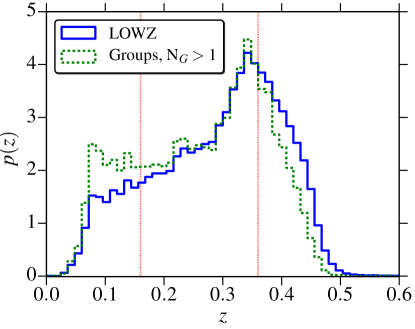
We use SDSS-III BOSS DR11 LOWZ galaxies, in the redshift range . The LOWZ sample consists of Luminous Red Galaxies (LRGs) at , selected from the SDSS DR8 imaging data and observed spectroscopically in BOSS survey. Fig. 1 shows the normalized redshift distribution of the LOWZ galaxies. The sample is approximately volume limited in the redshift range , with a number density of (Manera et al., 2014). We combine the spectroscopic redshifts from BOSS with galaxy shape measurements from Reyes et al. (2012). BOSS DR11 has 225334 LOWZ galaxies within our redshift range. However, due to higher Galactic extinction in some regions of the sky, Reyes et al. (2012) did not have shape measurements in those regions. After cutting out those regions, we are left with 173855 galaxies for our LOWZ density sample, of which there are good shape measurements for 159621 galaxies, which constitutes our LOWZ shape sample.
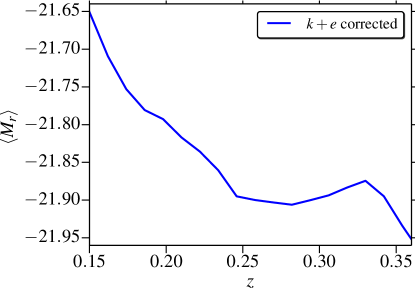
To compute absolute magnitudes, we use distances in the units of for distance modulus computation and then apply corrections (to ) as described in Wake et al. (2006). Fig. 2 shows the average corrected magnitudes as function of redshift. Throughout, we will use the corrected magnitudes.
To study the evolution of intrinsic alignments with redshift and different galaxy properties, we cut the LOWZ sample into different sub-samples. Table 2 describes the selection criteria and various properties of different sub-samples. Since our corrections are not perfect, we observe some redshift evolution in luminosity and color. To ensure that we select a fair samples based on luminosity and color cuts, those cuts are applied within redshift bins where each bin has 10 per cent of the sample (equal sized bins in redshift percentile space). We also observe evolution of color with luminosity but we avoid selecting color samples from luminosity bins, as that changes the redshift distribution () for different color samples, which complicates our correlation function calculations. For simplicity, we stick to redshift-based selection and keep the luminosity evolution in mind when interpreting the results for different color samples. Color and luminosity cuts are also based on percentile values. For example, the sample contains the galaxies in the percentile in luminosity within each bin. samples go from brightest to faintest, with – each containing 20% of the galaxies, and having the faintest 40 per cent of the galaxies ( has more galaxies to get sufficient S/N). Similarly each color sample has 20 per cent of the galaxies and go from blue to red end, with being the bluest and being the reddest.
| Dataset | Cuts | - | ||||||||
| Lowz | 173855 | 159621 | 0.28 | 0.95 | 1.18 | 13.180.05 | 4.60.5 | 1.770.04 | 0.080.01 | |
| BGG | , BGG=True | 19319 | 17916 | 0.27 | 1.31 | 1.16 | 13.50.1 | 8.11.5 | 2.540.13 | 0.410.05 |
| Group | 44780 | 40928 | 0.27 | 1.01 | 1.19 | 13.30.1 | 3.61.0 | 2.670.14 | 0.260.03 | |
| Satellite | , BGG=False | 25461 | 23012 | 0.27 | 0.78 | 1.22 | 13.10.1 | 01 | 2.770.15 | 0.160.04 |
| Field | 129075 | 118693 | 0.28 | 0.93 | 1.18 | 13.130.06 | 5.00.6 | 1.460.07 | 0.0110.007 | |
| Z1 | 67880 | 63180 | 0.21 | 0.91 | 1.17 | 13.170.06 | 4.10.8 | 1.660.07 | 0.050.01 | |
| Z2 | 105975 | 96441 | 0.32 | 0.98 | 1.19 | 13.180.07 | 5.10.8 | 1.880.05 | 0.160.02 | |
| 34760 | 31910 | 0.28 | 1.55 | 1.14 | 13.490.07 | 8.50.9 | 2.00.1 | 0.200.02 | ||
| 34768 | 31910 | 0.28 | 1.04 | 1.16 | 13.250.09 | 51 | 1.740.08 | 0.090.02 | ||
| 34768 | 31910 | 0.28 | 0.87 | 1.17 | 13.10.1 | 4.71.0 | 1.670.09 | 0.060.02 | ||
| 69530 | 63830 | 0.28 | 0.65 | 1.23 | 12.960.09 | 2.20.9 | 1.700.08 | 0.030.02 | ||
| 34760 | 31910 | 0.28 | 1.16 | 1.08 | 13.00.1 | 4.61.1 | 1.520.09 | 0.070.02 | ||
| 34768 | 31910 | 0.28 | 0.99 | 1.16 | 13.240.10 | 5.01.0 | 1.720.09 | 0.060.02 | ||
| 34768 | 31910 | 0.28 | 0.96 | 1.19 | 13.220.09 | 5.40.9 | 1.840.10 | 0.100.02 | ||
| 34768 | 31910 | 0.28 | 0.92 | 1.21 | 13.360.09 | 5.81.0 | 1.950.10 | 0.100.02 | ||
| 34760 | 31910 | 0.28 | 0.73 | 1.29 | 13.00.1 | 21 | 1.80.1 | 0.0790.025 |
Due to the finite size of the optical fibers required to target galaxies for spectroscopy, the SDSS is not able to simultaneously take spectra for galaxy pairs separated by on the sky. In regions of the sky which are observed multiple times (due to overlapping tiles), a number of such cases can be resolved. Nevertheless a significant fraction of targets remain unassigned. This effect is known as fiber collisions. Since fiber collisions occur preferentially in denser environments, the resulting incompleteness introduces a bias in correlation functions at all scales, with small scales being more strongly affected. One way to correct for this, is to upweight the nearest neighbor of a fiber collided galaxy. This is based on the assumption that two very nearby red sequence galaxies are likely to be within the same group or cluster. The nearest neighbor upweighting scheme has been shown to correct the bias in galaxy-galaxy correlation function on large scales ( fiber collision scale), but can introduce some bias at small scales since the redshift separation between the collided pair of galaxies has been artificially set to zero, which is not always correct (Reid et al., 2014). Also while measuring the clustering of galaxies in subsamples, the assumption that the fiber collided galaxy would also have been part of the same subsample as its nearest neighbor would be incorrect (see e.g., More et al., 2014, in the context of SDSS-III CMASS galaxies). Therefore, instead of upweighting the neighbors, we include the fiber collided galaxies in our sample, but assign them redshifts of their nearest neighbors. Nevertheless, bearing in mind sample incompleteness and fiber collision correction as possible source of systematics at small scales, we do not use the points below the fiber collision scale when fitting our models. Throughout, the fiber collision scale will be marked with solid black lines at kpc/h (fiber collision scale at ). In addition to the fiber collided galaxies, we also assign the nearest neighbor redshifts to galaxies for which the spectroscopic pipeline failed to obtain a redshift estimate. We calculate the absolute magnitudes along with corrections for these galaxies based on the nearest neighbor redshift estimates.
We use the sets of random points provided by the BOSS collaboration. However, some of our subsamples have different redshift distributions from the full LOWZ sample, in which case we generate new redshifts for the randoms from the subsample redshift distribution using the acceptance-rejection method. The acceptance-rejection method generates a set of random variates by uniformly sampling the area of the probability distribution of the random variable.
3.2 Shapes
The catalogue of galaxies with measured shapes used in this
paper (described in Reyes et al. 2012 and further characterized in Mandelbaum et al. 2013)
was generated using
the re-Gaussianization method (Hirata & Seljak, 2003) of
correcting for the effects of the point-spread function (PSF) on the
observed galaxy shapes. The catalogue production procedure was described in detail in previous work, so
we describe it only briefly here. Galaxies were selected in a 9243
deg2 region, with an average number density of arcmin-2.
The selection was based on cuts on the imaging quality, data reduction
quality, galactic extinction defined using the dust maps from
Schlegel, Finkbeiner & Davis (1998) and the extinction-to-reddening ratios from
Stoughton et al. (2002), apparent magnitude (extinction-corrected
), and galaxy size compared to the
PSF. The apparent magnitude cut used model
magnitudes666http://www.sdss3.org/dr8/algorithms/
magnitudes.php#mag_model. For comparing
the galaxy size to that of the PSF, we use the resolution factor
which is defined using the trace of the moment matrix of the PSF
and of the observed (PSF-convolved) galaxy image
as
| (30) |
We require in both and bands.
The software pipeline used to create this catalogue obtains galaxy images in the and filters from the SDSS ‘atlas images’ (Stoughton et al., 2002). The basic principle of shear measurement using these images is to fit a Gaussian profile with elliptical isophotes to the image, and define the components of the ellipticity
| (31) |
where is the axis ratio and is the position angle of the major axis. The ellipticity is then an estimator for the shear,
| (32) |
where is called the ‘shear responsivity’ and represents the response of the distortion to a small shear (Kaiser, Squires & Broadhurst, 1995; Bernstein & Jarvis, 2002); . In the course of the re-Gaussianization PSF-correction method, corrections are applied to account for non-Gaussianity of both the PSF and the galaxy surface brightness profiles (Hirata & Seljak, 2003).
For this work, we do not use the entire source catalogue, only the portion overlapping the LOWZ sample.
When computing the intrinsic alignment correlation functions, we use the shear estimates from this catalog together with the redshifts from BOSS. However, when computing the weak lensing signals around the LOWZ galaxies, we need estimates of the redshifts for the fainter source galaxies. For this purpose, we use the maximum-likelihood estimates of photometric redshifts (photo-) based on the five-band photometry from the Zurich Extragalactic Bayesian Redshift Analyzer (ZEBRA, Feldmann et al., 2006), which were characterized by Nakajima et al. (2012) and Reyes et al. (2012). In this work, we used a fair calibration sample of source galaxies with spectroscopic redshifts as defined in Nakajima et al. (2012) to calculate biases in weak lensing signals due to bias and scatter in the photo-, and applied corrections that were of order 10 per cent ( per cent) to the weak lensing signals.
3.3 Groups
We use the counts in cylinder (CiC) technique (Reid & Spergel, 2009) to find the galaxies in groups. The CiC technique assumes that for galaxies in the same halos, the dominant source of redshift separation between satellite and central galaxies are the line of sight relative velocities. Under such an assumption, a cylinder with size determined by the size and velocity dispersion of the halo should be able to identify galaxy pairs within a single halo. Reid & Spergel (2009) calibrated the CiC technique for halos hosting LRGs using mock LRG catalogs and we use their dimensions for the cylinders, given by and in comoving coordinates. Once within-halo pairs are identified, we can use the friends-of-friends algorithm to find all the galaxies belonging to the same group.
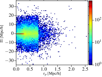
We note that the CiC parameters were optimized by Reid & Spergel (2009) for the SDSS LRG sample, and the LOWZ sample has a number density that is three times higher, extending to lower mass halos. Thus, using the CiC parameters optimized for LRG sample can potentially lead to spurious group identification in our LOWZ group sample. To roughly quantify the level of contamination, we use the halo mass function of Tinker et al. (2008) and find that the lower limit of halo mass for a sample of halos with the LOWZ sample abundance is a factor of less than a sample with the abundance of the LRG sample. Since the cylinder parameters should scale roughly like , this will give and for the LOWZ sample. Using these parameters, we find that the satellite fraction in LOWZ reduces to 11.7 per cent, versus 14.6 per cent using the CiC parameters from Reid & Spergel (2009). Most of this difference is coming from the reduction in the size, since most of the satellites are within as shown in Fig. 3. However, our calculation of CiC parameters for LOWZ is only approximate, as the CiC technique needs to be calibrated using mock catalogs, which is beyond the scope of this work. Hence for our science analysis we will use the group catalog obtained using CiC parameters of Reid & Spergel (2009) and we will discuss the impact of cylinder size on our conclusions in section 4.2.
Table 3 shows the multiplicity function of our group sample and Fig. 3 shows the stacked distribution of satellites with respect to BGGs, which we assume as the centre of groups. BGGs are selected as the brightest galaxy (in band) within the group. The assumption that the brightest galaxy truly resides at the center of the halo fails for about 25%-40% of the groups within our mass range (Skibba et al., 2011; Hikage et al., 2013), in which case the brightest galaxy is in fact a satellite galaxy. The mislabelling of the group center can suppress the radial alignment signal of satellite and also lead to spurious higher order moments in the measured correlation functions (see Schneider & Bridle 2010 for an illustration of this effect). Also, in low multiplicity groups (which dominate our group sample) the misidentification of a central but non-BGG galaxy as satellite can enhance the satellite alignment signal (under the assumption that central galaxies are more strongly aligned with halo shape as traced by satellites). These potential sources of contamination should be kept in mind when interpreting our results on the environmental dependence of intrinsic alignments.
1 130414 0.75 2 14944 0.17 3 2784 0.048 4 780 0.018 5 215 0.0062 6 84 0.0029 7 33 0.0013 8 17 0.00078 9 7 0.00036 10 2 0.00012 11 1 6.3 12 1 6.9 13 0 0 14 1 8.1 15 1 8.6
4 Results
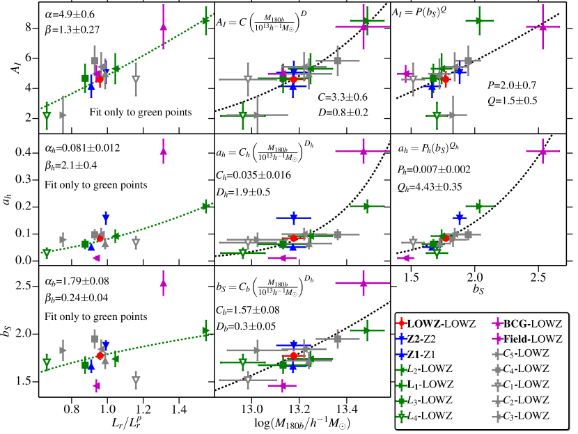
In this sections we present the results, beginning with correlation functions for full LOWZ sample and some tests for systematics. After that we primarily focus on evolution of intrinsic alignments amplitudes with different galaxy properties and end the section with some comparisons with other studies of intrinsic alignments, using different intrinsic alignments estimators where necessary. A summary of most of the results discussed in this section is presented in table 2 and Fig. 10.
4.1 LOWZ sample
We begin by showing our measurements for the full LOWZ sample. Fig. 4 shows our results for the galaxy-galaxy correlation function and the density-shape correlation function, . Throughout, when referring to two point correlation measurements, our naming convention for different results will be in the form of “Shape sample-Density sample”. We fit these data to the following models: the galaxy-galaxy correlation function calculated using non-linear matter power spectrum and linear galaxy bias, and the NLA model at . For the full LOWZ sample, we find a bias and intrinsic alignment amplitude . The NLA model is a good fit to the measurement for , and can be extended to , but there are significant deviations below that scale, due to differing scale dependence.
Our bias measurement appears to be in tension with results from Parejko et al. (2013), who measured for the BOSS DR9 LOWZ sample. However, there are a number of differences between our study and theirs: Parejko et al. (2013) (i) use a different redshift range, , (ii) use a smaller area DR9 sample, (iii) neglect redshift space distortions which can affect the large scale bias (see e.g., van den Bosch et al., 2013b), and (iv) use a FKP weighting scheme which favorably weights the large bias high redshift galaxies. Using the same redshift range as theirs, we also get a higher value of bias . When RSD corrections in our model are neglected, we obtain an even higher value of . We expect the remaining discrepancy to be a result of the further differences in the weighting scheme and/or the sample size. Our values are closer to the used by Tojeiro et al. (2014) in the reconstruction scheme for the BAO measurement (Tojeiro et al. 2014 use and ).
On non-linear scales, we use the halo model fitting formula for intrinsic alignments defined in Sec. 2.2, fitting to the data with . We find a good agreement with the data using the halo model parameters as described in Table 1, with halo model amplitude . Keeping fixed, but using fitting formula parameters from Schneider & Bridle (2010), the model does not fit data well. This is not surprising as the halo model fitting function does not explicitly model effects such as scale dependence of non-linear bias and intrinsic alignments themselves, which can change both the amplitude and scale dependence of the signal. For this reason and those described in Sec. 2.2, we caution against interpreting our values directly as an average intrinsic alignments shear.
The halo model fitting formula combined with the LA model (linear alignment model with linear matter power spectrum) does not fit the data well in the intermediate regime . Fig. 5 shows the joint fit to the sum of the halo model fitting function and the NLA model in the range . To better match the shape of the observed signal we let the parameter free in the halo model fitting function (in addition to the amplitude). We get best-fit values . The higher value of compared to the previous result, , is driven by the newly-included points below 6, while the value of is driven down by the small but non-negligible contributions from the NLA model below 1. The interpretation of this joint model is not clear, since it is possible that certain contributions to the signal are being double counted. Fitting our results to the NLA plus halo model fitting function with free shape parameter will permit us to fit many of the signals across a range of scales, but it also complicates the interpretation of the amplitude variations that we study later (variations in of the halo model fitting function also contribute to changes in ). For this reason, we do not show the combined fits for the NLA and halo model for other samples, but simply use the halo model fitting function as a convenient way to encapsulate the amplitude of the small-scale signal in a single number. For readers interested in self-consistent and uniform modeling using this ad hoc model at all scales, in Fig. 5 we also show the result of combining the one-parameter halo function with a smoothed NLA model (Blazek, McQuinn & Seljak, 2011) where the power spectrum in Eq. (3) is modified with a smoothing function as shown in Eq. (33), with smoothing scale /Mpc. Though not a very smooth function, this combination should provide a decent approximation to the measured signal at all scales as long as the halo model fitting function is valid (i.e. density sample is LOWZ):
| (33) |
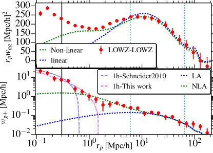
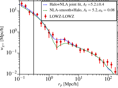
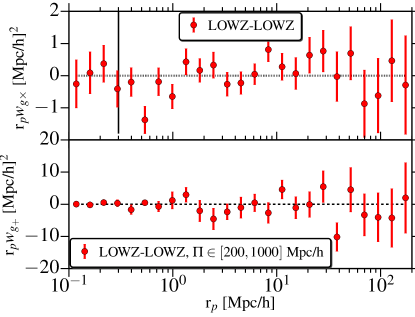
Fig. 6 shows our results for the measurement. The NLA model with the best-fitting parameters from predicts a small but non-zero . Our signal is dominated by shape noise, and our results (at ) marginally prefer the null model (best fit , with 8 bins, ,) over the NLA prediction using the amplitude from the fits to the signal () with a , which is not a statistically significant difference. Theoretically, from the NLA model with the best-fitting value of from the fits to , we expect (the ratio is scale dependent with a peak value of for ). In the shape noise-dominated limit, in the case that the shape and density sample are the same, the standard deviations of and are proportional to and (see, e.g., Schneider et al., 2002), respectively, where is the shape noise per component for our sample. For this sample, . Given a detection signal-to-noise ratio (SN) for on large scales of (), the expected SN for on large scales is then . Thus at we expect to have a null detection of , consistent with our observations. If we use scales below , the for a null signal777All -values in this paper calculated from either or use the simulation method described in Hirata et al. (2004) to account for the fact that the jackknife covariances are noisy, which modifies the expected distribution., with bins, giving a -value ().
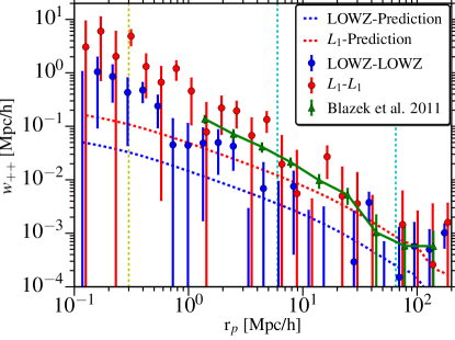
Our results are inconsistent with those for SDSS-I/II LRGs from Blazek, McQuinn & Seljak (2011) (, -value), as shown in Fig. 6. While calculating the projected correlation function from the 3d correlation functions in Okumura, Jing & Li (2009), Blazek, McQuinn & Seljak (2011) assumed isotropic along with Gaussian and independent errors. These assumptions are likely to break down at some level, and can cause a potential discrepancy with our results.
Other possible sources of the discrepancy are as follows. First, the LOWZ sample is fainter than the LRG sample in Blazek, McQuinn & Seljak (2011). Since the signal goes as , our expected signal is lower by a factor of (, ). Our sub-sample is closer to the LRG sample in term of luminosity and the number of galaxies. However, as shown in Fig. 6, the large scale signal for the sample is also consistent with a null signal (for , the best fit with for bins). The when we compare this with the value for the value from Blazek, McQuinn & Seljak (2011) is only . Hence our sample results do not rule out the Blazek, McQuinn & Seljak (2011) results; however, what is interesting is the very large discrepancy in the significance of detection between the two studies (with Blazek, McQuinn & Seljak 2011 ruling out the null model at high significance).
A possible explanation for this discrepancy in detection significance comes from the use of different per-galaxy shear estimates. The results in Okumura, Jing & Li (2009) that were used to present in Blazek, McQuinn & Seljak (2011) used isophotal shape measurements from the SDSS pipeline which are defined at a low surface brightness level and are not corrected for the effects of the PSF. PSF contamination and other systematics can introduce spurious shape correlations which can mimic a signal. However, it is still possible that we are seeing a real physical effect. The SDSS isophotal shape measurements emphasize the outer parts of galaxies, while re-Gaussianization puts more weight on the inner regions of galaxies. If the outer regions of galaxy shapes are more responsive to tidal fields, this could result in legitimately different signals when using the two different shear estimates. Using the MB-II SPH simulation, Tenneti et al. (2014b) found that differences in shape measurement methods, weighted towards outer or inner regions, leads to a difference of about 10% in the measurement888The trend is mass-dependent, and the difference is larger for lower mass. The number we quote here is for halo masses , which are the most appropriate ones for a comparison with massive galaxies like those in the LOWZ sample. (see also Schneider, Frenk & Cole, 2012; Allgood et al., 2006; Jing & Suto, 2002; Bett, 2012), which would translate to a difference in (with the right sign to explain what is seen here: is larger when weighting the outer regions more heavily). However, shape measurement methods in simulations may not correspond directly to shape measurement methods in observations and hence there may not be a direct correspondence between results from Tenneti et al. (2014b) and discrepancies observed between our results and that of Blazek, McQuinn & Seljak (2011). We also note that Blazek, McQuinn & Seljak (2011) detected signal as well, but our signal (not shown), like our signal, is consistent with zero. A definitive answer to this puzzle requires deeper analysis of shape measurement methods and their impact on IA measurement, which we defer to future work. Due to the null detection of in the LOWZ sample, we will not discuss hereafter.
4.2 Systematics tests
In this section, we present a measurement for the full LOWZ sample, and a measurement when integrating only over large values. Both these measurements are a good test for systematics in our shape measurements and correlation function calculations. From symmetry, is expected to be zero, while is also expected to have null signal when only large values are considered since the galaxy pairs are too far apart along the line-of-sight. As shown in Fig. 7, the signal is consistent with zero, with for bins (across all scales shown on the plot) and -value. at large values is also consistent with zero, with and -value. We therefore conclude that these signals, which could reveal possible systematic errors, are fully consistent with zero. There are also no patterns evident in the residuals from zero, just a slight hint that errorbars might be underestimated.
Fig. 8 shows the comparison of for two group samples with different CiC cylinder sizes. To test for the effect of our cylinder size choice, we make another group sample with cylinder size and (see Sec. 3.3 for reasons to choose alternative cylinder sizes) and compare the results with our main group sample as defined in Sec. 3.3. We find consistent values (well within ) for the linear bias and intrinsic alignments amplitudes and for all the samples used here (group, BGG, satellite, field). We do observe some differences in the small-scale clustering signal, which is probably due to some contamination of our main group sample by non-associated pairs. This does not affect any of our science results, and since the alternate group sample has not been validated with simulations, we will use the main group sample as defined in Sec. 3.3 for our science results.
4.3 Luminosity Dependence
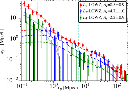
Previous studies using LRGs have observed luminosity dependence of intrinsic alignments (Hirata et al., 2007; Joachimi et al., 2011), where brighter galaxies tend to have higher intrinsic alignments amplitude. LOWZ sample allows us to study luminosity dependence by going to fainter luminosities, with spectroscopic redshifts for all galaxies. To study luminosity dependence, we divide the LOWZ sample into four sub-samples, based on -band absolute magnitude . The sample are defined according percentiles within bins (each bin has 10% of the sample). has the brightest 20% of the galaxies, followed by and samples which have next 20% galaxies each based on . has the faints 40% of the galaxies. Due to the decrease in signal to noise at fainter end, we do not cut sample into more sub-samples. Our density-shape correlation function measurements for the luminosity samples are shown in Fig. 9. All four samples are cross correlated with LOWZ as the density sample, and the LOWZ bias is fixed to (Sec. 4.1) when modeling the results. Fits to (not shown) reveal that the sample has the highest bias, followed by the , and samples though differences in last three samples are statistically not very significant(see Table 2 for values of fit parameters like the bias). However, the overall trend in the evolution of bias with luminosity is consistent with the fact that brighter galaxies live in more massive and hence more biased halos.
We also see luminosity variation of the intrinsic alignments amplitude and therefore of the NLA model best-fitting amplitude , with brighter galaxies having higher amplitude. Since the density sample is the same in each case, the increasing amplitude reflects the different intrinsic alignments for the different luminosity samples. Following Joachimi et al. (2011), we use a power law function to study the variation of with luminosity.
| (34) |
and are the -band luminosity and absolute magnitude, respectively, and is a pivot luminosity (magnitude), chosen to be . Fitting to the samples defined by our luminosity cuts, we find and slope (where these errors come from the jackknife). Our results are quite consistent with those of Joachimi et al. (2011), who found and (using MegaZ-LRG + SDSS LRG + L4 + L3), with the same k-corrections and choice of .
On small scales, we also see luminosity evolution of the halo model fitting function amplitude , with brighter galaxies having higher amplitude. Fitting a power law similar to Eq. (34), we find a power-law amplitude , and a power-law index (subscript “h” denotes fits to halo model fitting function parameters). The scaling of with luminosity is somewhat steeper than that of . This difference is likely due to that fact that more luminous galaxies live in denser regions, where tidal fields are stronger and hence leads to stronger intrinsic alignments (Pereira, Bryan & Gill, 2008). This will increase at all scales, but the impact will be much stronger at smaller scales, leading to stronger scaling of . This effect also contributes to the change in shape of for as the luminosity varies.
4.4 Redshift Dependence
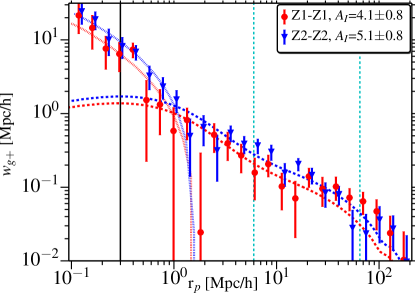
To study the redshift dependence of intrinsic alignments, we divide our sample into two redshift bins, Z1: , Z2: . Due to the small redshift range of the LOWZ sample, we cannot cut our samples further, as the edge effects from the redshift boundaries can then introduce significant bias in the correlation functions.
Fig. 11 shows the density-shape correlation measurements for both of the redshift samples. From measurement (not shown), we find higher galaxy bias for Z2 sample () compared to Z1 sample (), which is consistent with the fact that among halos of similar mass, ones at higher redshift are more biased. We do not find any redshift evolution for , which is consistent with the LA paradigm, where galaxy alignments are set at the time of galaxy formation and hence we do not expect any significant redshift evolution for intrinsic alignments beyond what is implicitly included due to use of a redshift-dependent nonlinear matter power spectrum that determines the gravitational tidal field. However, given the short redshift baseline, our power to constrain evolution of intrinsic alignments with redshift is limited.
On the small scales where we fit the halo model fitting function, there are significant differences between the two redshift ranges. The Z2 sample has a higher halo model amplitude. However, the Z2 sample is also expected to have a higher non-linear bias which will contribute to the increase in . Processes within groups and clusters, such as galactic mergers, stripping, peculiar motion and tidal torquing will also play an important role in determining the small scale signal (see, e.g. Pereira, Bryan & Gill, 2008) and can contribute to the redshift evolution of . Due to a degeneracy between intrinsic alignments amplitude and non-linear bias within the halo model, we cannot separate out the effects of these processes.
4.5 Color Dependence
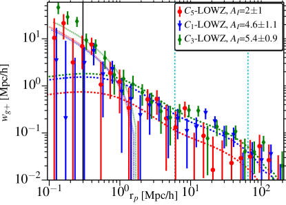
Our sample consists of only luminous red galaxies, so we cannot divide it into subsamples to study difference in intrinsic alignments for red and blue galaxies. However, we do split our sample based on color to study intrinsic alignments dependence on color within the LRG sample. We divide our sample into five sub-samples based on color, with each sample having 20 per cent of the LOWZ galaxies. Color cuts were applied in bins to take out the evolution of color and make sure we select a fair sample. The five samples, are arranged from the bluest to reddest. We observe significant luminosity evolution across the five samples, with redder samples getting progressively fainter. We do observe some intrinsic alignments evolution across the different samples, but find that the evolution can be well explained by the luminosity variations alone (see Fig. 12). We note that the sample is expected to have some contamination from late-type galaxies (Masters et al., 2011), but we do not observe a very significant deviation in intrinsic alignments signal from the expectation based on luminosity or mass scalings.
Our results suggests that luminosity and mass are more important properties in determining intrinsic alignments signal for red sequence galaxies, with color variations being absent or at least sub-dominant. This is an important test of the models that are commonly used to predict the intrinsic alignments contamination of future weak lensing surveys (e.g., Joachimi et al., 2011), which split galaxies into a red and a blue sample without permitting any variation in intrinsic alignments with color within those two samples. Our results validate this choice for the red galaxies, which are currently more important since they are the ones for which there is a robust intrinsic alignments detection.
4.6 Weak Lensing
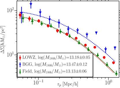
To study the halo mass dependence of intrinsic alignments, we compute the average halo mass of galaxies within different samples using galaxy-galaxy lensing. Figure 13 shows the weak lensing signal for LOWZ, BGG and field galaxies, with points being measurements from data and dashed lines are the NFW profile fits, with concentration fixed using concentration-mass relation defined in Eq. (29). The signal for BGGs deviates from an NFW profile for . These deviations could be due to some satellite contamination in our BGG sample, which is expected at the level of tens of per cent. At small scales, BGG mis-centering effects (which we have not accounted for in our fits) can also lead to deviations from the NFW profile resulting in underestimated halo mass.
To check for the effect of using fixed concentration-mass relation defined in Eq. (29), we vary the amplitude in Eq. (29) by and re-fit the signal from field sample, using (different from range used for main results). We find that the final mass measured changes by .
Mass measurements for different sample are given in table. 2. For full LOWZ sample, we get and for our brightest sample, , we get . Using the clustering analysis, Parejko et al. (2013) found for the DR9 LOWZ sample. Their masses correspond to FOF halos with a linking length of 0.2 which are expected to have a higher overdensity (see More et al., 2011), worsening the discrepancy we see here. However, clustering mass estimates are obtained in a less direct way that can have some bias due to modeling assumptions. Clustering and galaxy-galaxy lensing also have different redshift window functions and Parejko et al. (2013) used a different redshift range, , due to which it is hard to do a fair comparison between the two studies.
The second column in Fig. 10 shows the variations in intrinsic alignments amplitudes and galaxy bias as function of mass. As expected, more massive galaxies have higher bias, with the mass dependence of the bias being well-described by a power law, . Intrinsic alignments amplitudes are also strongly correlated with the mass, with more massive galaxies showing stronger intrinsic alignments. The relation between and mass can be well defined by a power law:
| (35) |
We find an amplitude and index . Similarly for the small scale amplitude , we get and index . However, this fit is significantly effected by the BGG-LOWZ correlation point, where BGG mass measurement are affected by satellite contamination and BGG mis-centering effects. Excluding the BGG-LOWZ point, we find and index . We also note that we can only test a small range in mass using our LOWZ sample, and this result is unlikely to be valid when extrapolated significantly outside this mass range.
4.7 Environment Dependence
One of the main goals of this work is to address the environmental dependence of intrinsic alignments. The halo model of intrinsic alignments (Schneider & Bridle, 2010) predicts that satellite galaxies tend to align radially within their host halos, while the BGGs tend to align with the halo shape, which itself tends to align with the large scale tidal gravitational field according to the linear alignment model. As described in Sec. 3.3, we identify galaxies in groups using the CiC technique and then separate them into satellites and BGGs. It is important to bear in mind that all results shown in this section for BGGs vs. satellites may be affected by the imperfect BGG selection, which will tend to dilute differences between the samples.
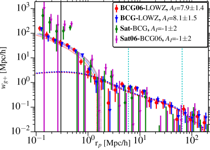
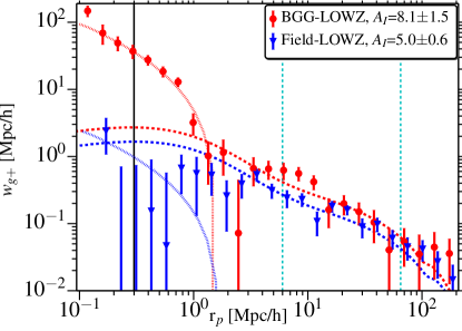
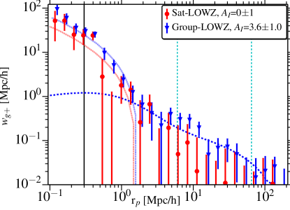
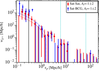
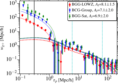
Figures 14 and 15 show our measurements for different combinations of galaxies within the groups and the field galaxies. In the plots, the density sample for both signals shown is the same, so the interpretation of large-scale amplitudes includes the same factor of density sample bias. At linear scales, we find that BGGs do tend to align with the tidal field and that BGG alignments are also stronger than that of field galaxies. This effect is consistent with the halo mass dependence of intrinsic alignments seen in Sec. 4.6, with BGGs living in more massive halos and thus showing stronger alignments. Satellite galaxies on the other hand, do not show any alignments at large scales, with . This is discrepant with the luminosity and mass relations of intrinsic alignments observed earlier, but consistent with the expectations from the halo model, where satellites are expected to be radially aligned within the halos and hence will have much weaker signal on large scales. Satellites are also the reason that the large-scale intrinsic alignments amplitude for group galaxies is lower than that of BGGs or even field galaxies.
At small scales, we detect a significant density-shape alignment signal for both satellite galaxies and BGGs. In the BGG-LOWZ correlation, the small scale signal is dominated by BGG-Group correlations (see also Fig. 18). In both cases what we are seeing is the fact that BGGs tend to point preferentially towards their own satellites or, equivalently, that the luminous red satellites of luminous red central galaxies are preferentially located along the major axes of their hosts. Also, in the satellite-LOWZ correlations, the primary contribution to the small scale signal is from within the groups as well, with satellite-BGG correlations (satellites pointing radially towards their hosts) being the dominant signal (see also Fig. 17). This confirms two of the assumptions made in the halo model: satellites do preferentially align radially within the halos, and BGGs preferentially align with the shape of their host halo. The signal observed in satellite-satellite correlations can also be explained by the combination of radial satellite alignments and the anisotropic distribution of satellites along the major axis of the host halo (Faltenbacher et al., 2007). The results shown in Figures 14 and 15 are likely to be affected by the contamination in our group sample due to our choice of CiC parameters (see discussion in Sec. 3.3), but the results in Figures 17 and 18 are more robust since most of the satellites are within of the BGG (see Fig. 3) and the signal for is not likely to be affected by the contamination in the group sample. We also note that even though our results do not agree with the null detection of satellite radial alignments in studies using cluster galaxies (e.g., Sifón et al., 2014; Schneider et al., 2013; Hao et al., 2011), our sample of LRGs is inherently different. The samples used in the group and cluster studies are dominated by fainter galaxies, which as shown in Sec. 4.3 have lower intrinsic alignments and hence lower the expected signal. Also, those samples are expected to have a small but non-negligible number of late type (blue/disk) galaxies for which intrinsic alignments may arise from angular momentum alignment, which is a second order effect (Hirata & Seljak, 2004). This will further weaken the likelihood of a detection of intrinsic alignments in the cluster studies. Hence, our detection of satellite radial alignments is not necessarily inconsistent with studies using cluster galaxies. Also see Sec. 4.10 for more discussion.
In Fig. 10, we also observe strong environmental dependence of the halo model fitting function amplitude . This result could potentially be contaminated by the effects of non-linear bias of the density sample which the halo model does not account for. We factor out this dependence by looking for variations in when the density sample of galaxies is fixed to LOWZ. As shown in Fig. 10, we fit a power law relation between halo model amplitude and linear galaxy bias, ,
| (36) |
We find amplitude and slope , in the bias range . We note that the power law dependence of small scale IA amplitude () on the large-scale linear bias () is not intuitively obvious. This relation implies that galaxies in more biased and hence more dense regions show higher intrinsic alignments at small scales, even though they are more likely to be effected by processes such galactic mergers and peculiar velocities which can potentially suppress the intrinsic alignments signal. This suggests that effects such as tidal torquing (which counteract mergers, boosting intrinsic alignments) do play an important role in determining intrinsic alignments at small scales.
Also, as described in Appendix A, what we measure is the density-weighted intrinsic shear . On small scales where the term cannot be neglected, the non-linear bias of shape sample (which is correlated with the large-scale linear bias ) will also contribute to produce correlations between and . These correlations will likely go as which is weaker than what we observe (). Thus, the intrinsic alignments at small scales are still driving the correlations between and . Given the small scatter in this relationship between and shown in Fig. 10, it is apparent that for a given sample of density tracers, the large-scale bias of the shape sample is the single best predictor of the small-scale intrinsic alignments amplitude considered in this work, better than luminosity or host halo mass. Note that the vs. halo mass relation shown in Fig. 10 is driven by the BGG-LOWZ data, where the BGG mass can be affected by satellite contamination and mis-centering effects as discussed in Sec. 4.6. However, that does not affect our conclusion that the large-scale bias is a more robust predictor of the small-scale amplitude than the galaxy luminosity. These results were all derived with a fixed density tracer sample; we relax this restriction in the following subsection.
4.8 Variation of intrinsic alignments with density sample
In this section, we address the question of whether alignments of galaxy shapes also depend on the density sample, i.e., do galaxy shapes tend to be more aligned with more massive or biased objects beyond the simple linear dependence on the bias of the density tracer sample. At linear scales, galaxies are biased tracers of large scale tidal fields and thus within the NLA regime we expect this effect to be negligible. Any changes in for the same shape sample and different density samples should be explained by variations in the bias of the density samples, and not by any changes in intrinsic alignments amplitude, . It is unlikely that the same should be true on small scales, where different density samples could have quite different nonlinear bias and environmental effects that will modify the intrinsic alignments beyond what is expected from the large-scale linear bias of the density tracer.
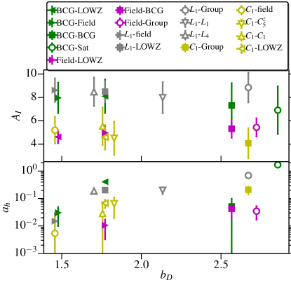
The top panel in Fig. 16 shows the variations in when a shape sample is correlated with different density samples. For a given shape sample, we do not find any significant changes in with different density samples. The largest change observed is for the field shape sample, where the difference in for field-LOWZ and field-group is , after accounting for the correlated errors (but see Fig. 21 for variations observed using a different estimator).
As described in Sec. 4.7, on small scales and especially within halos, more complex effects can be important in determining the intrinsic alignments signal for a given shape sample with different density samples. This effect is much harder to interpret using the 1-parameter halo model fitting function that we use in this work. As can be seen in Figs. 17 and 18, our fitting function does not fully capture the scale dependence of the small-scale signal once the density sample is different from the full LOWZ sample. This is not surprising, since we calibrated the shape of the fitting function to fit signals with LOWZ as the density sample. The scale dependence in the signal suggests that non-linear bias should have significant contributions to the scale dependence of intrinsic alignments signal. This effect, along with some possible variation of intrinsic alignments itself, can be captured if we let more free parameters in the fitting function, but the physical interpretation in that case is not very clear and we defer the study of such effects to future work. The bottom panel in Fig. 16 also shows the variations in the halo model fit to on small scales. There are significant deviations in observed with variations in the density sample, but as described earlier, it is hard to interpret these in terms of one parameter fitting function; a more detailed physical model is needed.
4.9 Putting it all together
In this section we briefly discuss and compare the scaling relations of intrinsic alignments amplitudes described earlier and shown in Fig. 10. For NLA amplitude, , we find that scalings with halo mass and luminosity are well described by a power law and scaling with bias is also well described by a linear fit though with larger scatter. All of these scaling are consistent with the observation that more luminous galaxies, living in more massive halos have stronger alignments. It is interesting to note that scaling with luminosity is stronger than scaling with mass, though we caution that mass and luminosity are correlated. To check if this difference in scaling index has any physical meaning, we fit a power law of of the form to mass and luminosity of different samples. We get , which compares well with the expectation from simply comparing scalings, . From this we can conclude that these scaling represent same underlying physical effect and one can use either mass or luminosity to predict intrinsic alignments amplitude at large scale. We also note that when fitting for vs scaling, including all the points shown in Fig. 10, the parameters donot change significantly ( and ), which further strengthens our conclusion that either mass or luminosity of sample can be used to predict intrinsic alignments amplitude.
We also find similar mass and luminosity scaling for the halo model amplitude and we can also draw similar conclusions that both mass and luminosity scaling present same underlying physical effect. It is also interesting to note that mass and luminosity scaling indices for are higher than that for , though scatter is also higher. The correlation with linear galaxy bias for is also much stronger, with linear galaxy bias being much better predictor of than mass or luminosity, within the narrow range of our sample. Since the scaling relations with mass/luminosity are steeper for than for , this implies that the radial () dependence of the intrinsic alignments on kpc to tens of Mpc scales must be changing as the mass/luminosity change. Thus, a single template for intrinsic alignment radial dependence will be insufficient to model intrinsic alignments for future surveys.
As discussed in Sec. 4.5 and Sec. 4.4, we do not detect any significant redshift or color evolution of intrinsic alignments amplitudes within the limited range of values probed by our sample (red sequence galaxies in the range ). However, galaxy properties like mass, luminosity and bias may also depend slightly on the redshift and color. Any such evolution of these properties and intrinsic alignments amplitudes is self-consistently explained by the scaling relations discussed above and we do not detect any additional redshift or color dependence.
To summarize, we find that the best (lowest scatter) predictor of the large-scale intrinsic alignments signal for a given shape sample is the galaxy luminosity or mass (not its linear bias), whereas the lowest- scatter predictor of the small-scale intrinsic alignments signal for a given shape sample is the linear bias (not its luminosity or mass). However, the shape and amplitude of the small-scale intrinsic alignments signal also depends on the choice of density-tracer sample in a non-trivial way, whereas the large-scale signal only depends in a simple (linear) way on the linear bias of the density sample.
4.10 Comparison with other works
Different studies have used a variety of estimators to measure the intrinsic alignments of galaxies. To compare with their results and also to test for compatibility of different estimators, we present our results using two more estimators, and .
| (37) |
| (38) |
is as defined in Sec. 2.3. is the angle between the projected major axis of the shape galaxy and the line joining the pair of galaxies. measures the average intrinsic shear of the galaxies, while measures the tendency of galaxies to align in the direction of other galaxies. In the absence of intrinsic alignments, will be consistent with zero while will tend to a value of 45∘. In case of radial alignments, will be less than 45∘ and will be positive.
Both and are measured with a single bin in the range . Unless stated otherwise, we take .
Figure 19 shows our measurement of both and for the full LOWZ sample. There is good agreement with the three estimators in terms of scale dependence, with 1-halo to 2-halo transitions around clearly observable in all three estimators. The flattening of and at small scales is due to the fact that in taking average, normalization is done by while in it is done by . Since at small scales there are more galaxy pairs than would be expected for a random galaxy distribution, the small scale slope for is steeper than for and . The flattening of the signal at could also partly be due to contamination from fiber collision galaxies that we have included in our sample, which can potentially bring the signal down if the fiber collision correction is wrong. Note that similar values of and is a coincidence. They represent very different measurements, and similarities in their magnitudes does not have any physical meaning.
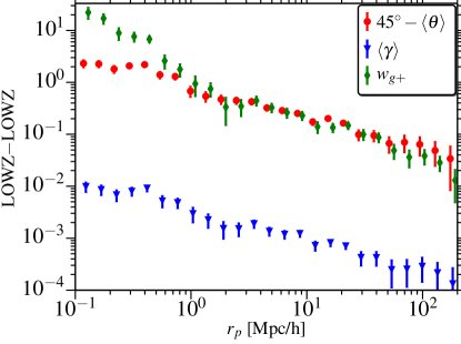
Fig. 20 shows the satellite-BGG and BGG-satellite correlations. In this case, we fix , so that the signal at small scales, is only for galaxies within the groups. Our choice of range here is the same as in Sec. 3.3, to select the galaxy pairs within the groups (given that the apparent size of groups along the line of sight is determined by the Fingers of God effect). Sifón et al. (2014) measured the satellite-BGG correlations using spectroscopically selected member for clusters and found a null signal, with . For our sample, we find satellite radial shear , for scales . To provide a plausible explanation for this discrepancy, we assume that the power-law relation between halo model amplitude and -band magnitude in Fig. 10 can be extrapolated outside of the luminosity range of the LOWZ sample and can also be extended to measurement for Sat-BCG type correlations. This assumption, coupled with the fact that galaxies used by Sifón et al. (2014) are on average magnitude fainter than LOWZ galaxies, implies that the expected signal for Sifón et al. (2014) is lower than our by a factor of (allowing for some possible variations in luminosity scaling), which is well within the size of their errors. Also, disturbed and late type (blue) galaxies in Sifón et al. (2014) sample will further bring down the expected signal, but their galaxies reside in more massive halos, which could push the signal up again. We speculate that, with these two effects acting in opposite direction, the expected signal in Sifón et al. (2014) sample will still be lower than observed in our sample.
For , averaging over , we find for satellite-BGG correlations and for BGG-satellite correlations with While satellites and BGGs tend to point towards each other, the effect is stronger for BGGs pointing towards satellites rather than the reverse. Though these results suffer from contamination in our group sample due to our choice of CiC parameters (see discussion in Sec. 3.3), the results in Fig. 20 as function of are robust since most satellites are within of the BGGs (see Fig. 3).
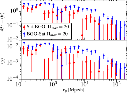
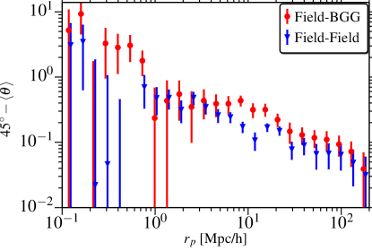
Fig. 21 shows a measurement of for field galaxies, correlated with other field galaxies (blue) and BGGs (red). is higher for field-BGG than field-field, which suggests that field galaxies have higher tendency to point towards groups than towards other field galaxies. Averaging over , we get for field-BGG and for field-field correlations (errors are correlated since the shape sample is the same in both cases.). The deviation from a strict amplitude rescaling, manifested as a change in shape around , is likely from filamentary structures, with field galaxies residing in filaments around the groups and hence having higher tendency to align with the groups. This result is qualitatively consistent with the findings of Zhang et al. (2013), who used SDSS DR7 data to reconstruct tidal fields and found that galaxies within filaments tend to have their major axis preferentially aligned with the direction of the filament. More generally, this observation implies that there is a mass dependent sphere of influence within which gravity can align the shapes of galaxies, with BGGs having a larger sphere of influence due to the fact that they reside in higher-mass halos.
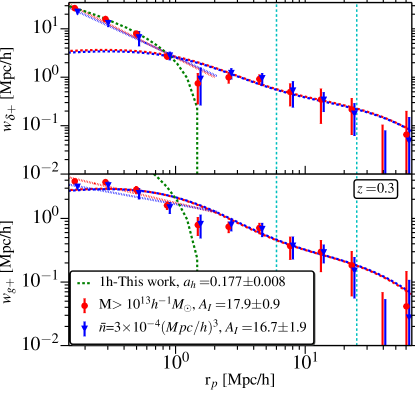
Fig. 22 shows results from Tenneti et al. (2014b) for and measurements from the MB-II hydrodynamical simulation, at redshift . We show results from two different samples, the first of which is defined by a halo mass threshold (blue) and the second by a luminosity threshold giving a fixed comoving number density of ()3. in Tenneti et al. (2014b) is measured using the shapes of galaxies as defined using the star particles (for those galaxies with star particles), with dark matter subhalos as density tracers (), while for , dark matter particles are the density tracers (). Both and are fit simultaneously at linear scales, assuming they have the same but different . On non-linear scales, Tenneti et al. (2014b) fit a simple power law. The NLA model intrinsic alignments amplitudes are higher for these simulated samples than for LOWZ. The mass threshold sample is comparable to our and BGG samples in terms of average halo mass, but its intrinsic alignments are higher than what we observe for these samples by a factor of two. The luminosity threshold sample has a comoving number density similar to the full LOWZ sample, but LOWZ has lower by a factor of .
There are several possibilities that could explain the discrepancy between simulations and observations. The first possibility is some unrealistic aspect of the simulations, including an atypical galaxy shape distribution or a higher degree of alignment between dark matter halo and galaxy shapes than in reality. The second possibility is that this comparison is not completely fair due to the way the galaxy samples were selected in MB-II. For example, the LOWZ sample has a color cut but the simulated samples do not; in real data we are rejecting some massive galaxies that are even slightly blue and including some lower mass red galaxies, but this effect is not included in the simulated samples. Also, a mass-selected sample is unrealistic because our mass tracer (luminosity) is known to have a quite high scatter with mass. Moreover, if this scatter is not present at the same level in the simulated luminosities, that will drastically change the nature of the simulated samples in the direction of having too high average mass and intrinsic alignments. We therefore cannot draw any conclusions from the disagreement in amplitude. However, it is encouraging that despite the difference in selection, the scaling of with in simulations and the LOWZ observations are comparable. This suggests that the simulations are likely successful in modeling the basic physical processes that cause the intrinsic alignments, even if the magnitude is not quite correct.
5 Conclusions
We have studied intrinsic alignments in SDSS-III BOSS low redshift (LOWZ) galaxies by combining spectroscopic redshifts from BOSS with shape measurements from Reyes et al. (2012). Using this sample, we have made a robust detection of intrinsic alignments from to scales. We find that the NLA model (linear alignment model with non-linear power spectrum) fits the data well for , though there are significant deviations at smaller scales. At small scales, we also fitted the data with a halo model-based fitting formula, and find that as long as the density tracer sample is fixed, the intrinsic alignments for different shape samples can be described by simply varying the halo model amplitude, i.e. different shape samples do not introduce any significant scale dependence of their own. However, variations in density samples changes the scale dependence on scales due to changes in the non-linear bias for different samples.
We also studied the luminosity dependence of intrinsic alignments, finding significant evolution of intrinsic alignments with luminosity, with brighter galaxies having stronger intrinsic alignments. For the density sample comprising of LOWZ galaxies, the luminosity dependence of the intrinsic alignments can be well described by a power law fit in luminosity, with power law slope of for (NLA model amplitude) and for the small-scale halo model fitting function amplitude. While extrapolation beyond the range of luminosities explored here must be done cautiously, this luminosity dependence likely has important implications for future surveys like LSST and Euclid, which will go to much fainter magnitudes than SDSS, and hence overall intrinsic alignments contamination for shear studies in such surveys should go down. This, however, does not mean that intrinsic alignments contamination will not be important as the statistical error budget for these surveys is also far smaller than for SDSS.
We calculated the average halo mass of galaxies in various samples using weak lensing and then studied the mass dependence of intrinsic alignments. We find that the intrinsic alignments amplitude (on both small and large scales) increases with halo mass, and the mass-intrinsic alignments amplitude relations are well described by a power law in mass. This result is consistent with luminosity evolution as well and taken together, both luminosity and mass evolutions imply that brighter and more massive galaxies show stronger intrinsic alignments.
We do not find any significant redshift dependence of intrinsic alignments within the limited range of . This is consistent with the linear alignment model, which assumes that intrinsic alignments are imprinted at earlier times during the formation of galaxy. Other effects at later times can in principle introduce some redshift dependence, but the effect seems to be too small to be detected in our narrow redshift range.
We also do not find any significant evolution of intrinsic alignments with color, within the red sequence. We split the sample into 5 color bins with each bin containing 20 per cent of the LOWZ sample. There is some luminosity evolution within our color samples, and any intrinsic alignments variation that we see within these samples can be explained by the luminosity scalings.
We identified the galaxies in groups using the CiC technique as described in Sec. 3.3 and studied the environment dependence of intrinsic alignments. We find large scale alignments for BGGs in our sample as well as strong alignments of BGGs shapes with satellites. Our results are consistent with the halo model as well as observations from simulations where BGGs are found to be aligned with their host dark matter halos (as traced by satellites), which in turn have large scale alignments as described by linear alignment model. We also detect small scale alignments of satellite shapes, consistent with radial alignments assumed in halo model and observed in simulations (this conclusion is based on the assumption that BGGs are the center of halos). We reiterate that the CiC parameters used in this work were optimized for the higher mass SDSS LRG sample, not the LOWZ sample. This could potentially lead to some contamination in our group sample. However, based on our estimates of the importance of this effect, it does not significantly affect our overall conclusions about the environmental dependence of intrinsic alignments.
Finally, comparison with previous studies using a variety of estimators suggests that our results are either in good agreement or the differences can be explained by differences in the sample selection, most notably the average luminosity of the galaxies.
To summarize, our results suggest that mass and luminosity are the most important factors in determining the intrinsic alignments of red galaxies, with color (within the red sequence) and redshift effects being subdominant. The best predictor (least scatter) for intrinsic alignments at large scales is the halo mass/luminosity of the galaxies, while at small scales, the (large-scale) linear bias is the best predictor assuming that the density tracer sample is kept fixed. Comparing our halo fitting function and NLA amplitudes to those observed in simulations should help in better understanding of processes involved in galaxy formation and how baryonic matter and dark matter influence each other within the halos. Moreover, our results and constraints on the NLA model and the small-scale fitting function should also be useful in putting priors on models of intrinsic alignments used in mitigation schemes (see for example, King, 2005; Bridle & King, 2007; Joachimi & Bridle, 2010) for upcoming large surveys that aim to use weak lensing to measure the equation of state of dark energy to extremely high precision.
6 Acknowledgements
This work was supported by the National Science Foundation under Grant. No. AST-1313169. RM was also supported by an Alfred P. Sloan Fellowship. SM is supported by World Premier International Research Center Initiative (WPI Initiative), MEXT, Japan, by the FIRST program “Subaru Measurements of Images and Redshifts (SuMIRe)”, CSTP, Japan. We thank Benjamin Joachimi, Alina Kiessling, Marcello Cacciato, Jonathan Blazek, and Cristobal Sifón for useful discussions about this work. We thank the anonymous referee for useful feedback that improved the paper.
Funding for SDSS-III has been provided by the Alfred P. Sloan Foundation, the Participating Institutions, the National Science Foundation, and the U.S. Department of Energy Office of Science. The SDSS-III web site is http://www.sdss3.org/.
SDSS-III is managed by the Astrophysical Research Consortium for the Participating Institutions of the SDSS-III Collaboration including the University of Arizona, the Brazilian Participation Group, Brookhaven National Laboratory, Carnegie Mellon University, University of Florida, the French Participation Group, the German Participation Group, Harvard University, the Instituto de Astrofisica de Canarias, the Michigan State/Notre Dame/JINA Participation Group, Johns Hopkins University, Lawrence Berkeley National Laboratory, Max Planck Institute for Astrophysics, Max Planck Institute for Extraterrestrial Physics, New Mexico State University, New York University, Ohio State University, Pennsylvania State University, University of Portsmouth, Princeton University, the Spanish Participation Group, University of Tokyo, University of Utah, Vanderbilt University, University of Virginia, University of Washington, and Yale University.
References
- Abazajian et al. (2009) Abazajian K. N. et al., 2009, ApJS, 182, 543
- Ahn et al. (2012) Ahn C. P. et al., 2012, ApJS, 203, 21
- Aihara et al. (2011) Aihara H. et al., 2011, ApJS, 193, 29
- Allgood et al. (2006) Allgood B., Flores R. A., Primack J. R., Kravtsov A. V., Wechsler R. H., Faltenbacher A., Bullock J. S., 2006, MNRAS, 367, 1781
- Basilakos et al. (2006) Basilakos S., Plionis M., Yepes G., Gottlöber S., Turchaninov V., 2006, MNRAS, 365, 539
- Bernstein & Jarvis (2002) Bernstein G. M., Jarvis M., 2002, AJ, 123, 583
- Bett (2012) Bett P., 2012, MNRAS, 420, 3303
- Blanton et al. (2003) Blanton M. R., Lin H., Lupton R. H., Maley F. M., Young N., Zehavi I., Loveday J., 2003, AJ, 125, 2276
- Blazek et al. (2012) Blazek J., Mandelbaum R., Seljak U., Nakajima R., 2012, JCAP, 5, 41
- Blazek, McQuinn & Seljak (2011) Blazek J., McQuinn M., Seljak U., 2011, JCAP, 5, 10
- Bolton et al. (2012) Bolton A. S. et al., 2012, AJ, 144, 144
- Bridle & King (2007) Bridle S., King L., 2007, New Journal of Physics, 9, 444
- Capranico, Merkel & Schäfer (2013) Capranico F., Merkel P. M., Schäfer B. M., 2013, MNRAS, 435, 194
- Catelan, Kamionkowski & Blandford (2001) Catelan P., Kamionkowski M., Blandford R. D., 2001, MNRAS, 320, L7
- Chisari & Dvorkin (2013) Chisari N. E., Dvorkin C., 2013, JCAP, 12, 29
- Chisari et al. (2014) Chisari N. E., Mandelbaum R., Strauss M. A., Huff E. M., Bahcall N. A., 2014, MNRAS, 445, 726
- Crittenden et al. (2001) Crittenden R. G., Natarajan P., Pen U.-L., Theuns T., 2001, ApJ, 559, 552
- Croft & Metzler (2000) Croft R. A. C., Metzler C. A., 2000, ApJ, 545, 561
- Dawson et al. (2013) Dawson K. S. et al., 2013, AJ, 145, 10
- Eisenstein et al. (2001) Eisenstein D. J. et al., 2001, AJ, 122, 2267
- Faltenbacher et al. (2008) Faltenbacher A., Jing Y. P., Li C., Mao S., Mo H. J., Pasquali A., van den Bosch F. C., 2008, ApJ, 675, 146
- Faltenbacher et al. (2007) Faltenbacher A., Li C., Mao S., van den Bosch F. C., Yang X., Jing Y. P., Pasquali A., Mo H. J., 2007, ApJ, 662, L71
- Feldmann et al. (2006) Feldmann R. et al., 2006, MNRAS, 372, 565
- Forero-Romero, Contreras & Padilla (2014) Forero-Romero J. E., Contreras S., Padilla N., 2014, MNRAS, 443, 1090
- Fukugita et al. (1996) Fukugita M., Ichikawa T., Gunn J. E., Doi M., Shimasaku K., Schneider D. P., 1996, AJ, 111, 1748
- Gunn et al. (1998) Gunn J. E. et al., 1998, AJ, 116, 3040
- Gunn et al. (2006) Gunn J. E. et al., 2006, AJ, 131, 2332
- Hao et al. (2011) Hao J., Kubo J. M., Feldmann R., Annis J., Johnston D. E., Lin H., McKay T. A., 2011, ApJ, 740, 39
- Heymans et al. (2006) Heymans C., White M., Heavens A., Vale C., van Waerbeke L., 2006, MNRAS, 371, 750
- Hikage et al. (2013) Hikage C., Mandelbaum R., Takada M., Spergel D. N., 2013, MNRAS, 435, 2345
- Hinshaw et al. (2013) Hinshaw G. et al., 2013, ApJS, 208, 19
- Hirata & Seljak (2003) Hirata C., Seljak U., 2003, MNRAS, 343, 459
- Hirata et al. (2007) Hirata C. M., Mandelbaum R., Ishak M., Seljak U., Nichol R., Pimbblet K. A., Ross N. P., Wake D., 2007, MNRAS, 381, 1197
- Hirata et al. (2004) Hirata C. M. et al., 2004, MNRAS, 353, 529
- Hirata & Seljak (2004) Hirata C. M., Seljak U., 2004, Phys.Rev.D, 70, 063526
- Hogg et al. (2001) Hogg D. W., Finkbeiner D. P., Schlegel D. J., Gunn J. E., 2001, AJ, 122, 2129
- Hopkins, Bahcall & Bode (2005) Hopkins P. F., Bahcall N. A., Bode P., 2005, ApJ, 618, 1
- Hung & Ebeling (2012) Hung C.-L., Ebeling H., 2012, MNRAS, 421, 3229
- Ivezić et al. (2004) Ivezić Ž. et al., 2004, Astronomische Nachrichten, 325, 583
- Jing & Suto (2002) Jing Y. P., Suto Y., 2002, ApJ, 574, 538
- Joachimi & Bridle (2010) Joachimi B., Bridle S. L., 2010, A&A, 523, A1
- Joachimi et al. (2011) Joachimi B., Mandelbaum R., Abdalla F. B., Bridle S. L., 2011, A&A, 527, A26
- Joachimi et al. (2013a) Joachimi B., Semboloni E., Bett P. E., Hartlap J., Hilbert S., Hoekstra H., Schneider P., Schrabback T., 2013a, MNRAS, 431, 477
- Joachimi et al. (2013b) Joachimi B., Semboloni E., Hilbert S., Bett P. E., Hartlap J., Hoekstra H., Schneider P., 2013b, MNRAS, 436, 819
- Kaiser (1987) Kaiser N., 1987, MNRAS, 227, 1
- Kaiser, Squires & Broadhurst (1995) Kaiser N., Squires G., Broadhurst T., 1995, ApJ, 449, 460
- Kang et al. (2007) Kang X., van den Bosch F. C., Yang X., Mao S., Mo H. J., Li C., Jing Y. P., 2007, MNRAS, 378, 1531
- Khandai et al. (2014) Khandai N., Di Matteo T., Croft R., Wilkins S. M., Feng Y., Tucker E., DeGraf C., Liu M.-S., 2014, arXiv, 1402.0888
- King (2005) King L. J., 2005, A&A, 441, 47
- Knebe et al. (2008) Knebe A., Draganova N., Power C., Yepes G., Hoffman Y., Gottlöber S., Gibson B. K., 2008, MNRAS, 386, L52
- Kuhlen, Diemand & Madau (2007a) Kuhlen M., Diemand J., Madau P., 2007a, ApJ, 671, 1135
- Kuhlen, Diemand & Madau (2007b) Kuhlen M., Diemand J., Madau P., 2007b, ApJ, 671, 1135
- Landy & Szalay (1993) Landy S. D., Szalay A. S., 1993, ApJ, 412, 64
- Laureijs et al. (2011) Laureijs R. et al., 2011, arXiv, 1110.3193
- Lewis & Bridle (2002) Lewis A., Bridle S., 2002, Phys. Rev., D66, 103511
- LSST Science Collaboration et al. (2009) LSST Science Collaboration et al., 2009, arXiv, 0912.0201
- Lupton et al. (2001) Lupton R., Gunn J. E., Ivezić Z., Knapp G. R., Kent S., 2001, in Astronomical Society of the Pacific Conference Series, Vol. 238, Astronomical Data Analysis Software and Systems X, Harnden Jr. F. R., Primini F. A., Payne H. E., eds., p. 269
- Mandelbaum et al. (2011) Mandelbaum R. et al., 2011, MNRAS, 410, 844
- Mandelbaum et al. (2006) Mandelbaum R., Hirata C. M., Ishak M., Seljak U., Brinkmann J., 2006, MNRAS, 367, 611
- Mandelbaum et al. (2005) Mandelbaum R. et al., 2005, MNRAS, 361, 1287
- Mandelbaum, Seljak & Hirata (2008) Mandelbaum R., Seljak U., Hirata C. M., 2008, JCAP, 8, 6
- Mandelbaum et al. (2013) Mandelbaum R., Slosar A., Baldauf T., Seljak U., Hirata C. M., Nakajima R., Reyes R., Smith R. E., 2013, MNRAS, 432, 1544
- Manera et al. (2014) Manera M. et al., 2014, arXiv, 1401.4171
- Masters et al. (2011) Masters K. L. et al., 2011, MNRAS, 418, 1055
- More et al. (2011) More S., Kravtsov A. V., Dalal N., Gottlöber S., 2011, ApJS, 195, 4
- More et al. (2014) More S., Miyatake H., Mandelbaum R., Takada M., Spergel D., Brownstein J., Schneider D. P., 2014, arXiv, 1407.1856
- Nakajima et al. (2012) Nakajima R., Mandelbaum R., Seljak U., Cohn J. D., Reyes R., Cool R., 2012, MNRAS, 420, 3240
- Navarro, Frenk & White (1996) Navarro J. F., Frenk C. S., White S. D. M., 1996, ApJ, 462, 563
- Norberg et al. (2009) Norberg P., Baugh C. M., Gaztañaga E., Croton D. J., 2009, MNRAS, 396, 19
- Okumura, Jing & Li (2009) Okumura T., Jing Y. P., Li C., 2009, ApJ, 694, 214
- Padmanabhan et al. (2008) Padmanabhan N. et al., 2008, ApJ, 674, 1217
- Parejko et al. (2013) Parejko J. K. et al., 2013, MNRAS, 429, 98
- Pereira, Bryan & Gill (2008) Pereira M. J., Bryan G. L., Gill S. P. D., 2008, ApJ, 672, 825
- Pier et al. (2003) Pier J. R., Munn J. A., Hindsley R. B., Hennessy G. S., Kent S. M., Lupton R. H., Ivezić Ž., 2003, AJ, 125, 1559
- Ragone-Figueroa et al. (2010) Ragone-Figueroa C., Plionis M., Merchán M., Gottlöber S., Yepes G., 2010, MNRAS, 407, 581
- Reid et al. (2014) Reid B. A., Seo H.-J., Leauthaud A., Tinker J. L., White M., 2014, MNRAS, 444, 476
- Reid & Spergel (2009) Reid B. A., Spergel D. N., 2009, ApJ, 698, 143
- Reyes et al. (2012) Reyes R., Mandelbaum R., Gunn J. E., Nakajima R., Seljak U., Hirata C. M., 2012, MNRAS, 425, 2610
- Richards et al. (2002) Richards G. T. et al., 2002, AJ, 123, 2945
- Schlegel, Finkbeiner & Davis (1998) Schlegel D. J., Finkbeiner D. P., Davis M., 1998, ApJ, 500, 525
- Schneider & Bridle (2010) Schneider M. D., Bridle S., 2010, MNRAS, 402, 2127
- Schneider et al. (2013) Schneider M. D. et al., 2013, MNRAS, 433, 2727
- Schneider, Frenk & Cole (2012) Schneider M. D., Frenk C. S., Cole S., 2012, JCAP, 5, 30
- Schneider et al. (2002) Schneider P., van Waerbeke L., Kilbinger M., Mellier Y., 2002, A&A, 396, 1
- Sheldon et al. (2004) Sheldon E. S. et al., 2004, AJ, 127, 2544
- Sifón et al. (2014) Sifón C., Hoekstra H., Cacciato M., Viola M., Köhlinger F., van der Burg R., Sand D., Graham M. L., 2014, arXiv, 1406.5196
- Skibba et al. (2011) Skibba R. A., van den Bosch F. C., Yang X., More S., Mo H., Fontanot F., 2011, MNRAS, 410, 417
- Smee et al. (2013) Smee S. A. et al., 2013, AJ, 146, 32
- Smith et al. (2002) Smith J. A. et al., 2002, AJ, 123, 2121
- Smith et al. (2003) Smith R. E. et al., 2003, MNRAS, 341, 1311
- Spergel et al. (2013) Spergel D. et al., 2013, arXiv, 1305.5422
- Springel et al. (2005) Springel V. et al., 2005, Nature, 435, 629
- Stoughton et al. (2002) Stoughton C. et al., 2002, AJ, 123, 485
- Strauss et al. (2002) Strauss M. A. et al., 2002, AJ, 124, 1810
- Tenneti et al. (2014a) Tenneti A., Mandelbaum R., Di Matteo T., Feng Y., Khandai N., 2014a, MNRAS, 441, 470
- Tenneti et al. (2014b) Tenneti A., Singh S., Mandelbaum R., Di Matteo T., Feng Y., Khandai N., 2014b, arXiv, 1409.7297
- Tinker et al. (2008) Tinker J., Kravtsov A. V., Klypin A., Abazajian K., Warren M., Yepes G., Gottlöber S., Holz D. E., 2008, ApJ, 688, 709
- Tojeiro et al. (2014) Tojeiro R. et al., 2014, MNRAS, 440, 2222
- Troxel & Ishak (2014) Troxel M. A., Ishak M., 2014, ArXiv e-prints
- Tucker et al. (2006) Tucker D. L. et al., 2006, Astronomische Nachrichten, 327, 821
- van den Bosch et al. (2013a) van den Bosch F. C., More S., Cacciato M., Mo H., Yang X., 2013a, MNRAS, 430, 725
- van den Bosch et al. (2013b) van den Bosch F. C., More S., Cacciato M., Mo H., Yang X., 2013b, MNRAS, 430, 725
- Velander et al. (2014) Velander M. et al., 2014, MNRAS, 437, 2111
- Wake et al. (2006) Wake D. A. et al., 2006, MNRAS, 372, 537
- Wang et al. (2011) Wang H., Mo H. J., Jing Y. P., Yang X., Wang Y., 2011, MNRAS, 413, 1973
- Weinberg et al. (2013) Weinberg D. H., Mortonson M. J., Eisenstein D. J., Hirata C., Riess A. G., Rozo E., 2013, Phys.Rep., 530, 87
- York et al. (2000) York D. G. et al., 2000, AJ, 120, 1579
- Zhang et al. (2015) Zhang Y., Yang X., Wang H., Wang L., Luo W., Mo H. J., van den Bosch F. C., 2015, ApJ, 798, 17
- Zhang et al. (2013) Zhang Y., Yang X., Wang H., Wang L., Mo H. J., van den Bosch F. C., 2013, ApJ, 779, 160
Appendix A Effect of Redshift space distortions on intrinsic alignments
The effect of redshift space distortions on the galaxy clustering signal was first studied by Kaiser (1987). In this appendix we show the effect of redshift space distortions on the intrinsic alignment correlation functions. For simplicity, we will consider configuration space, assume that the plane parallel approximation holds, and that the direction corresponds to the line-of-sight. The following coordinate transformation maps real space to redshift space,
| (39) |
where the primed quantities correspond to redshift space, we have assumed units with , is the magnitude of the velocity at the real space position (positive value corresponds to motion away from the observer) and is the cosine of the angle between the velocity and the line-of-sight.
Let us begin by considering the quantity which is the intrinsic alignment of a shape sample of galaxies with respect to matter in real space. Since the intrinsic shear is measured at the position of the shape sample of galaxies, in practice, we measure the density-weighted intrinsic shear, , where
| (40) |
where is the overdensity of the shape sample of galaxies and its bias with respect to the matter density fluctuation . The last equality follows from the proportionality (see Equation 2), and from the Poisson equation. Here is the matter density fluctuation. Thus if we restrict to linear order (as we will throughout this appendix), there is no correction to the intrinsic shear due to the density weighted measurement. Therefore, we will not make a distinction between the intrinsic shear and its density weighted counterpart, hereafter.
In this appendix we will work out the relation between and the corresponding redshift space quantity, . Since the shear distortion comes from the tidal field at the true position of the galaxy, and is unchanged by redshift-space distortions, the only effect of RSD is to change the apparent position of the galaxy. This will result in its contributing to the 3D correlation function or at a different value of , but without changing the intrinsic shear value itself. and are therefore related by
| (41) |
The Fourier transform of the left hand side gives
| (42) |
where . We can combine this term and expand the exponential as a Taylor series to obtain
| (43) |
Here we have used , where the last two equalities are valid at linear order. Therefore,
| (44) |
This implies that there is no linear order correction to the intrinsic shear field while going from real to redshift space.
Now consider a density sample characterized by its overdensity . Number density conservation relates the redshift space overdensity to the real space overdensity such that
| (45) |
Therefore,
| (46) |
The linear order correction of when going from real coordinates to redshift coordinates is valid both in configuration and Fourier space.
The auto-power spectrum of the intrinsic shear and its cross power spectrum with the galaxy overdensity field in redshift space and real space are therefore related by
| (47) | ||||
| (48) |
while the galaxy-galaxy power spectrum in real and redshift space are related by
| (49) |