Some Invariant String Cosmological Models in Cylindrically Symmetric Space-time

Ahmad T Ali1,†, Anil Kumar Yadav2 , Farook Rahaman3 and Arkopriya Mallick4

1 King Abdul Aziz University, Faculty of Science, Department of Mathematics,

PO Box 80203, Jeddah, 21589, Saudi Arabia.

E-mail: atali71@yahoo.com

Mathematics Department, Faculty of Science, Al-Azhar University,

Nasr city, 11884, Cairo, Egypt

2 Department of Physics, Anand Engineering College, Keetham, Agra - 282 007, India.

E-mail: abanilyadav@yahoo.co.in

3 Department of Mathematics, Jadavpur University, Kolkata 700 032, India.

E-mail: rahaman@iucaa.ernet.in

4 Department of Mathematics, Jadavpur University, Kolkata 700 032, India.

E-mail: arkopriyamallick@gmail.com

Abstract

In this paper we derive some new invariant solutions of Einstein-Maxwell’s field equations for string fluid as source of matter in cylindrically symmetric space-time with Variable Magnetic Permeability. We also discuss the physical and geometrical properties of the models derived in the paper. The solutions, at least one of them, are interesting physically as they can explain the accelerating as well as singularity free Universe.

PACS: 98.80.JK, 98.80.-k.

Keywords: Similarity solutions, Magnetized cylindrically symmetric space-time, Inhomogeneous cosmological model, General Relativity.

1 Introduction

One of the important consequence of general theory of relativity is to know the large scale structure of the Universe. The study of cosmology is devoted to the Universe as a whole. Initial study was based on FRW type which describes the space which is homogeneous and isotropic. We know homogeneity and isotropy are symmetries of space. Though the present observations indicates that the Universe is almost perfectly homogeneous and isotropic in large scales,, however, the symmetries of space in very early Universe could be very different. Today s observations could not able to provide information about symmetries of space near initial singularity. Hence, it is very justified to consider inhomogeneous and anisotropic models of the Universe. Cylindrically-symmetric space-time is more general than the homogeneous and isotropic space-time and plays an important role in the study of the universe when the anisotropy and inhomogeneity are taking into consideration. Barrow and Kunze [1, 2] investigated flat and open homogeneous universe, considering string fluid as source of matter. In the recent past, Pradhan et al [3] and Yadav et al [4] have studied inhomogeneous cosmological models with cloud of strings; the latter were invoked to palliate the problems associated with cylindrically symmetric space-time.

Due to non-linearity, general theory of relativity is a very difficult theory. Therefore, to describe the models of the Universe, different group of symmetries are used in literature. In this study, we apply the so-called symmetry analysis method. The main advantage of this method is that it can be successfully applied to nonlinear differential equations. The similarity solutions are attractive because they result in the reduction of the independent variables of the problem. In our case, the problem under investigation is the system of second order nonlinear PDEs and similarity solution will transform this system of nonlinear PDEs into a system of ODEs.

The groups of continuous transformations that leave a given family of equations invariant is known as symmetry groups (isovector fields) [5, 6, 7, 8, 9]. In a pioneering work, Ovsiannikov [10] mentioned that the usual Lie infinitesimal invariance approach could as well be employed in order to construct symmetry groups [11, 12, 13].

In recent years , there has been considerable interest in string cosmology. Cosmic string plays an important role in the study of the early universe. String cosmology is a relatively new field that tries to apply equation of string theory to solve the questions of early cosmology , a related area of study in brain cosmology. It was argued by Melvin [14] that the presence of magnetic field is not as unrealistic because for a large part of the history of evolution matter was highly ionized and matter and field were smoothly coupled. Latter during the expansion of the Universe, the ions combined to form neutral matter. Therefore, inclusion of the magnetic field with Variable Magnetic Permeability is justified for cosmological modeling of the Universe.

In this paper, we attempted to find a new class of exact (similarity) solutions for string cosmological models in cylindrically symmetric inhomogeneous universe with electro magnetic perfect fluid distribution with variable magnetic permeability in general relativity.

We organize the paper as follows: String cosmological model in cylindrically symmetric inhomogeneous universe with electro-magnetic perfect fluid distribution of variable magnetic permeability in general relativity, is introduced in section 2. In section 3, symmetry analysis and isovector fields for Einstein field equations are obtained. In section 4, we find a new class of exact (similarity) solutions for Einstein field equations. Section 5 is devoted to the study of some physical and geometrical properties of the obtained model. The paper ends with a short discussion.

2 The metric and field equations

We consider the metric in the form

ds2=A2(dx2dt2)+B2dy2+C2dz2,𝑑superscript𝑠2superscript𝐴2𝑑superscript𝑥2𝑑superscript𝑡2superscript𝐵2𝑑superscript𝑦2superscript𝐶2𝑑superscript𝑧2ds^{2}=A^{2}\,\big{(}dx^{2}-dt^{2}\big{)}+B^{2}\,dy^{2}+C^{2}\,dz^{2}, (1)

where A𝐴A, B𝐵B and C𝐶C are functions of x𝑥x and t𝑡t. The energy-momentum tensor for the string with electro-magnetic field has the form

Tij=ρuiujλxixj+Eij,subscript𝑇𝑖𝑗𝜌subscript𝑢𝑖subscript𝑢𝑗𝜆subscript𝑥𝑖subscript𝑥𝑗subscript𝐸𝑖𝑗T_{ij}=\rho\,u_{i}\,u_{j}-\lambda\,x_{i}\,x_{j}+E_{ij}, (2)

where uisubscript𝑢𝑖u_{i} and xisubscript𝑥𝑖x_{i} satisfy the conditions

uiui=xixi=1,superscript𝑢𝑖subscript𝑢𝑖superscript𝑥𝑖subscript𝑥𝑖1u^{i}\,u_{i}\,=\,-x^{i}\,x_{i}\,=\,-1, (3)

and

uixi= 0.superscript𝑢𝑖subscript𝑥𝑖 0u^{i}\,x_{i}\,=\,0. (4)

Here ρ𝜌\rho being the rest energy density of the system of strings, λ𝜆\lambda the tension density of the strings , xisuperscript𝑥𝑖x^{i} is a unit space-like vector representing the direction of strings so that x1=x2=x4=0superscript𝑥1superscript𝑥2superscript𝑥40x^{1}=x^{2}=x^{4}=0 and x30superscript𝑥30x^{3}\neq 0, and uisuperscript𝑢𝑖u^{i} is the four velocity vector. Eijsubscript𝐸𝑖𝑗E_{ij} is the electro-magnetic field given by Lichnerowicz [15]:

Eij=μ¯[hlhl(uiuj+12gij)hihj],subscript𝐸𝑖𝑗¯𝜇delimited-[]subscript𝑙superscript𝑙subscript𝑢𝑖subscript𝑢𝑗12subscript𝑔𝑖𝑗subscript𝑖subscript𝑗E_{ij}=\bar{\mu}\big{[}h_{l}h^{l}\big{(}u_{i}u_{j}+\frac{1}{2}g_{ij}\big{)}-h_{i}h_{j}\big{]}, (5)

where μ¯¯𝜇\bar{\mu} is the magnetic permeability and hisubscript𝑖h_{i} the magnetic flux vector defined by:

hi=1μ¯Fjiuj,subscript𝑖superscript1¯𝜇subscript𝐹𝑗𝑖superscript𝑢𝑗h_{i}=\dfrac{1}{\bar{\mu}}\,^{*}F_{ji}\,u^{j}, (6)

where the dual electro-magnetic field tensor Fijsuperscriptsubscript𝐹𝑖𝑗{}^{*}F_{ij} is defined by Synge [16]

Fij=g2ϵijklFkl.^{*}F_{ij}=\dfrac{\sqrt{-g}}{2}\,\epsilon_{ijkl}\,F^{kl}. (7)

Here Fijsubscript𝐹𝑖𝑗F_{ij} is the electro-magnetic field tensor and ϵijklsubscriptitalic-ϵ𝑖𝑗𝑘𝑙\epsilon_{ijkl} is a Levi-Civita tensor density. In the present scenario, the co-moving coordinates are taken as

ui=(0,0,0,1A).superscript𝑢𝑖0001𝐴u^{i}=\Big{(}0,0,0,\dfrac{1}{A}\Big{)}. (8)

We choose the direction of string parallel to x𝑥x-axis so that

xi=(1A,0,0,0).superscript𝑥𝑖1𝐴000x^{i}=\Big{(}\dfrac{1}{A},0,0,0\Big{)}. (9)

If we consider the current flow along z𝑧z-axis, then F12subscript𝐹12F_{12} is only non-vanishing component of Fijsubscript𝐹𝑖𝑗F_{ij}. Then the Maxwell’s equations

Fij;k+Fjk;i+Fki;j=0subscript𝐹𝑖𝑗𝑘subscript𝐹𝑗𝑘𝑖subscript𝐹𝑘𝑖𝑗0F_{ij;k}+F_{jk;i}+F_{ki;j}=0 (10)

and

[1μ¯Fij];j=Ji\Big{[}\dfrac{1}{\bar{\mu}}F^{ij}\Big{]}_{;j}=J^{i} (11)

require that F12subscript𝐹12F_{12} be function of x𝑥x alone [17]. We assume that the magnetic permeability as a function of both x𝑥x and t𝑡t. Here the semicolon represents a covariant differentiation.

The Einstein’s field equation

Rij12gijR=χTij,subscript𝑅𝑖𝑗12subscript𝑔𝑖𝑗𝑅𝜒subscript𝑇𝑖𝑗R_{ij}-\dfrac{1}{2}\,g_{ij}\,R=-\chi\,T_{ij}, (12)

for the line-element (1) lead to the following system of equations:

CxtC+BxtBAtCx+AxCtACAtBx+AxBtAB=0,subscript𝐶𝑥𝑡𝐶subscript𝐵𝑥𝑡𝐵subscript𝐴𝑡subscript𝐶𝑥subscript𝐴𝑥subscript𝐶𝑡𝐴𝐶subscript𝐴𝑡subscript𝐵𝑥subscript𝐴𝑥subscript𝐵𝑡𝐴𝐵0missing-subexpression\begin{array}[]{ll}\dfrac{C_{xt}}{C}+\dfrac{B_{xt}}{B}-\dfrac{A_{t}\,C_{x}+A_{x}\,C_{t}}{A\,C}-\dfrac{A_{t}\,B_{x}+A_{x}\,B_{t}}{A\,B}=0,\end{array} (13)
CxxCtt2C+BxxBtt2B+AxxAttA+At2Ax2A2=0,subscript𝐶𝑥𝑥subscript𝐶𝑡𝑡2𝐶subscript𝐵𝑥𝑥subscript𝐵𝑡𝑡2𝐵subscript𝐴𝑥𝑥subscript𝐴𝑡𝑡𝐴superscriptsubscript𝐴𝑡2superscriptsubscript𝐴𝑥2superscript𝐴20missing-subexpression\begin{array}[]{ll}\dfrac{C_{xx}-C_{tt}}{2\,C}+\dfrac{B_{xx}-B_{tt}}{2\,B}+\dfrac{A_{xx}-A_{tt}}{A}+\dfrac{A_{t}^{2}-A_{x}^{2}}{A^{2}}=0,\end{array} (14)
χA2λ=CxxC+BttB+AxxAttA+BtCtBxCxBCAtCt+AxCxACAxBx+AtBtAB+At2Ax2A2,𝜒superscript𝐴2𝜆subscript𝐶𝑥𝑥𝐶subscript𝐵𝑡𝑡𝐵subscript𝐴𝑥𝑥subscript𝐴𝑡𝑡𝐴subscript𝐵𝑡subscript𝐶𝑡subscript𝐵𝑥subscript𝐶𝑥𝐵𝐶missing-subexpressionmissing-subexpressionmissing-subexpressionsubscript𝐴𝑡subscript𝐶𝑡subscript𝐴𝑥subscript𝐶𝑥𝐴𝐶subscript𝐴𝑥subscript𝐵𝑥subscript𝐴𝑡subscript𝐵𝑡𝐴𝐵superscriptsubscript𝐴𝑡2superscriptsubscript𝐴𝑥2superscript𝐴2missing-subexpression\begin{array}[]{ll}\chi\,A^{2}\,\lambda=\dfrac{C_{xx}}{C}+\dfrac{B_{tt}}{B}+\dfrac{A_{xx}-A_{tt}}{A}+\dfrac{B_{t}\,C_{t}-B_{x}\,C_{x}}{B\,C}\\ \\ \,\,\,\,\,\,\,\,\,\,\,\,\,\,\,\,\,\,\,\,\,\,\,\,\,\,\,\,\,\,\,\,\,\,\,\,\,\,\,\,\,\,\,\,\,\,\,\,\,\,-\dfrac{A_{t}\,C_{t}+A_{x}\,C_{x}}{A\,C}-\dfrac{A_{x}\,B_{x}+A_{t}\,B_{t}}{A\,B}+\dfrac{A_{t}^{2}-A_{x}^{2}}{A^{2}},\end{array} (15)
χA2ρ=Ctt2CxxCBttB+AttAxxA+BtCtBxCxBC+AtCt+AxCxAC+AxBx+AtBtAB+Ax2At2A2,𝜒superscript𝐴2𝜌subscript𝐶𝑡𝑡2subscript𝐶𝑥𝑥𝐶subscript𝐵𝑡𝑡𝐵subscript𝐴𝑡𝑡subscript𝐴𝑥𝑥𝐴subscript𝐵𝑡subscript𝐶𝑡subscript𝐵𝑥subscript𝐶𝑥𝐵𝐶missing-subexpressionmissing-subexpressionmissing-subexpressionsubscript𝐴𝑡subscript𝐶𝑡subscript𝐴𝑥subscript𝐶𝑥𝐴𝐶subscript𝐴𝑥subscript𝐵𝑥subscript𝐴𝑡subscript𝐵𝑡𝐴𝐵superscriptsubscript𝐴𝑥2superscriptsubscript𝐴𝑡2superscript𝐴2missing-subexpression\begin{array}[]{ll}\chi\,A^{2}\,\rho=\dfrac{C_{tt}-2\,C_{xx}}{C}-\dfrac{B_{tt}}{B}+\dfrac{A_{tt}-A_{xx}}{A}+\dfrac{B_{t}\,C_{t}-B_{x}\,C_{x}}{B\,C}\\ \\ \,\,\,\,\,\,\,\,\,\,\,\,\,\,\,\,\,\,\,\,\,\,\,\,\,\,\,\,\,\,\,\,\,\,\,\,\,\,\,\,\,\,\,\,\,\,\,\,\,\,+\dfrac{A_{t}\,C_{t}+A_{x}\,C_{x}}{A\,C}+\dfrac{A_{x}\,B_{x}+A_{t}\,B_{t}}{A\,B}+\dfrac{A_{x}^{2}-A_{t}^{2}}{A^{2}},\end{array} (16)
χF1222μ¯B2=CxxCttC+AxxAttA+At2Ax2A2,𝜒superscriptsubscript𝐹1222¯𝜇superscript𝐵2subscript𝐶𝑥𝑥subscript𝐶𝑡𝑡𝐶subscript𝐴𝑥𝑥subscript𝐴𝑡𝑡𝐴superscriptsubscript𝐴𝑡2superscriptsubscript𝐴𝑥2superscript𝐴2missing-subexpression\begin{array}[]{ll}\dfrac{\chi\,F_{12}^{2}}{2\,\bar{\mu}\,B^{2}}=\dfrac{C_{xx}-C_{tt}}{C}+\dfrac{A_{xx}-A_{tt}}{A}+\dfrac{A_{t}^{2}-A_{x}^{2}}{A^{2}},\end{array} (17)

The velocity field uisuperscript𝑢𝑖u^{i} is ir-rotational. The scalar expansion ΘΘ\Theta, shear scalar σ2superscript𝜎2\sigma^{2}, acceleration vector u˙isubscript˙𝑢𝑖\dot{u}_{i} and Proper volume V𝑉V are respectively found to have the following expressions [18, 19]:

Θ=u;ii=1A(CtC+BtB+AtA),\Theta\,=\,u_{;i}^{i}=\dfrac{1}{A}\Big{(}\dfrac{C_{t}}{C}+\dfrac{B_{t}}{B}+\dfrac{A_{t}}{A}\Big{)}, (18)
σ2=12σijσij=Θ231A2(BtCtBC+AtCtAC+AtBtAB),superscript𝜎212subscript𝜎𝑖𝑗superscript𝜎𝑖𝑗superscriptΘ231superscript𝐴2subscript𝐵𝑡subscript𝐶𝑡𝐵𝐶subscript𝐴𝑡subscript𝐶𝑡𝐴𝐶subscript𝐴𝑡subscript𝐵𝑡𝐴𝐵missing-subexpression\begin{array}[]{ll}\sigma^{2}\,=\,\dfrac{1}{2}\,\sigma_{ij}\,\sigma^{ij}=\dfrac{\Theta^{2}}{3}-\dfrac{1}{A^{2}}\Big{(}\dfrac{B_{t}\,C_{t}}{B\,C}+\dfrac{A_{t}\,C_{t}}{A\,C}+\dfrac{A_{t}\,B_{t}}{A\,B}\Big{)},\end{array} (19)
u˙i=ui;juj=(AxA,0,0,0),subscript˙𝑢𝑖subscript𝑢𝑖𝑗superscript𝑢𝑗subscript𝐴𝑥𝐴000\dot{u}_{i}\,=\,u_{i;j}\,u^{j}\,=\,\Big{(}\dfrac{A_{x}}{A},0,0,0\Big{)}, (20)
V=g=A2BC,𝑉𝑔superscript𝐴2𝐵𝐶V=\sqrt{-g}=A^{2}\,B\,C, (21)

where g𝑔g is the determinant of the metric (1). The shear tensor is

σij=u(i;j)+u˙(iuj)13Θ(gij+uiuj).\begin{array}[]{ll}\sigma_{ij}\,=\,u_{(i;j)}+\dot{u}_{(i}\,u_{j)}-\frac{1}{3}\,\Theta\,(g_{ij}+u_{i}\,u_{j}).\end{array} (22)

and the non-vanishing components of the σijsuperscriptsubscript𝜎𝑖𝑗\sigma_{i}^{j} are

{σ11=13A(2AtABtBCtC),σ22=13A(2BtBCtC+AtA),σ33=13A(2CtCBtB+AtA),σ44=0.casessuperscriptsubscript𝜎11absent13𝐴2subscript𝐴𝑡𝐴subscript𝐵𝑡𝐵subscript𝐶𝑡𝐶missing-subexpressionmissing-subexpressionsuperscriptsubscript𝜎22absent13𝐴2subscript𝐵𝑡𝐵subscript𝐶𝑡𝐶subscript𝐴𝑡𝐴missing-subexpressionmissing-subexpressionsuperscriptsubscript𝜎33absent13𝐴2subscript𝐶𝑡𝐶subscript𝐵𝑡𝐵subscript𝐴𝑡𝐴missing-subexpressionmissing-subexpressionsuperscriptsubscript𝜎44absent0\left\{\begin{array}[]{ll}\sigma_{1}^{1}&=\,\dfrac{1}{3\,A}\Big{(}\dfrac{2\,A_{t}}{A}-\dfrac{B_{t}}{B}-\dfrac{C_{t}}{C}\Big{)},\\ \\ \sigma_{2}^{2}&=\,\dfrac{1}{3\,A}\Big{(}\dfrac{2\,B_{t}}{B}-\dfrac{C_{t}}{C}+\dfrac{A_{t}}{A}\Big{)},\\ \\ \sigma_{3}^{3}&=\,\dfrac{1}{3\,A}\Big{(}\dfrac{2\,C_{t}}{C}-\dfrac{B_{t}}{B}+\dfrac{A_{t}}{A}\Big{)},\\ \\ \sigma_{4}^{4}&=0.\end{array}\right. (23)

Using the field equations and the relations (18) and (19) one obtains the Raychaudhuri’s equation is

Θt=u˙;iiΘ232σ2ρp2,\begin{array}[]{ll}\dfrac{\partial\Theta}{\partial t}=\dot{u}_{;i}^{i}-\dfrac{\Theta^{2}}{3}-2\,\sigma^{2}-\dfrac{\rho_{p}}{2},\end{array} (24)

where

ρp=2Rijuiuj.subscript𝜌𝑝2subscript𝑅𝑖𝑗superscript𝑢𝑖superscript𝑢𝑗missing-subexpression\begin{array}[]{ll}\rho_{p}=2\,R_{ij}\,u^{i}\,u^{j}.\end{array} (25)

The Einstein field equations (13)-(17) constitute a system of five highly non-linear differential equations with six unknowns variables, A𝐴A, B𝐵B, C𝐶C, λ𝜆\lambda, ρ𝜌\rho and F122μ¯superscriptsubscript𝐹122¯𝜇\frac{F_{12}^{2}}{\bar{\mu}}. Therefore, one physically reasonable conditions amongst these parameters are required to obtain explicit solutions of the field equations. Let us assume that the expansion scalar ΘΘ\Theta in the model (1) is proportional to the eigenvalue σ11superscriptsubscript𝜎11\sigma_{1}^{1} of the shear tensor σjksuperscriptsubscript𝜎𝑗𝑘\sigma_{j}^{k}. Then from (18) and (23), we get

2AtABtBCtC=3γ(AtA+BtB+CtC),2subscript𝐴𝑡𝐴subscript𝐵𝑡𝐵subscript𝐶𝑡𝐶3𝛾subscript𝐴𝑡𝐴subscript𝐵𝑡𝐵subscript𝐶𝑡𝐶missing-subexpression\begin{array}[]{ll}\dfrac{2\,A_{t}}{A}-\dfrac{B_{t}}{B}-\dfrac{C_{t}}{C}=3\,\gamma\,\Big{(}\dfrac{A_{t}}{A}+\dfrac{B_{t}}{B}+\dfrac{C_{t}}{C}\Big{)},\end{array} (26)

where γ𝛾\gamma is a constant of proportionality. The above equation can be written in the form

AtA=n(BtB+CtC).subscript𝐴𝑡𝐴𝑛subscript𝐵𝑡𝐵subscript𝐶𝑡𝐶missing-subexpression\begin{array}[]{ll}\dfrac{A_{t}}{A}\,=n\,\Big{(}\dfrac{B_{t}}{B}+\dfrac{C_{t}}{C}\Big{)}.\end{array} (27)

where n=1+3γ23γ𝑛13𝛾23𝛾n=\dfrac{1+3\,\gamma}{2-3\,\gamma}. If we integrate the above equation with respect to t𝑡t, we can get the following relation

A(x,t)=f(x)(B(x,t)C(x,t))n,𝐴𝑥𝑡𝑓𝑥superscript𝐵𝑥𝑡𝐶𝑥𝑡𝑛missing-subexpression\begin{array}[]{ll}A(x,t)\,=\,f(x)\,\Big{(}B(x,t)\,C(x,t)\Big{)}^{n},\end{array} (28)

where f(x)𝑓𝑥f(x) is a constant of integration which is an arbitrary function of x𝑥x. If we substitute the metric function A𝐴A from (20) in the Einstein field equations, the equations (13)-(14) transform to the nonlinear partial differential equations of the coefficients B𝐵B and C𝐶C only, as the following new form:

E1=BxtB+CxtC2n(BxBtB2+BxCt+BtCxBC+CxCtC2)ff(BtB+CtC)=0,subscript𝐸1subscript𝐵𝑥𝑡𝐵subscript𝐶𝑥𝑡𝐶2𝑛subscript𝐵𝑥subscript𝐵𝑡superscript𝐵2subscript𝐵𝑥subscript𝐶𝑡subscript𝐵𝑡subscript𝐶𝑥𝐵𝐶subscript𝐶𝑥subscript𝐶𝑡superscript𝐶2superscript𝑓𝑓subscript𝐵𝑡𝐵subscript𝐶𝑡𝐶0missing-subexpression\begin{array}[]{ll}E_{1}=\dfrac{B_{xt}}{B}+\dfrac{C_{xt}}{C}-2\,n\,\Big{(}\dfrac{B_{x}\,B_{t}}{B^{2}}+\dfrac{B_{x}\,C_{t}+B_{t}\,C_{x}}{B\,C}+\dfrac{C_{x}\,C_{t}}{C^{2}}\Big{)}-\dfrac{f^{\prime}}{f}\Big{(}\dfrac{B_{t}}{B}+\dfrac{C_{t}}{C}\Big{)}=0,\end{array} (29)
E2=(n+12)[BxxBttB+CxxCttC]+n(Bt2Bx2B2+Ct2Cx2C2)+f′′ff2f2=0,subscript𝐸2𝑛12delimited-[]subscript𝐵𝑥𝑥subscript𝐵𝑡𝑡𝐵subscript𝐶𝑥𝑥subscript𝐶𝑡𝑡𝐶𝑛superscriptsubscript𝐵𝑡2superscriptsubscript𝐵𝑥2superscript𝐵2superscriptsubscript𝐶𝑡2superscriptsubscript𝐶𝑥2superscript𝐶2superscript𝑓′′𝑓superscript𝑓2superscript𝑓20missing-subexpression\begin{array}[]{ll}E_{2}=\Big{(}n+\dfrac{1}{2}\Big{)}\Big{[}\dfrac{B_{xx}-B_{tt}}{B}+\dfrac{C_{xx}-C_{tt}}{C}\Big{]}+n\Big{(}\dfrac{B_{t}^{2}-B_{x}^{2}}{B^{2}}+\dfrac{C_{t}^{2}-C_{x}^{2}}{C^{2}}\Big{)}+\dfrac{f^{\prime\prime}}{f}-\dfrac{f^{\prime 2}}{f^{2}}=0,\end{array} (30)

where the prime indicates derivative with respect to the coordinate x𝑥x.

3 Symmetry analysis method

In order to obtain an exact solutions of the system of nonlinear partial differential equations (29)-(30), we will use the symmetry analysis method. For this we write

{xi=xi+ϵξi(xj,uβ)+𝕠(ϵ2),uα=uα+ϵηα(xj,uβ)+𝕠(ϵ2),i,j,α,β=1,2,formulae-sequencecasessuperscriptsubscript𝑥𝑖subscript𝑥𝑖italic-ϵsubscript𝜉𝑖subscript𝑥𝑗subscript𝑢𝛽𝕠superscriptitalic-ϵ2missing-subexpressionsuperscriptsubscript𝑢𝛼subscript𝑢𝛼italic-ϵsubscript𝜂𝛼subscript𝑥𝑗subscript𝑢𝛽𝕠superscriptitalic-ϵ2missing-subexpression𝑖𝑗𝛼𝛽12\left\{\begin{array}[]{ll}x_{i}^{*}=x_{i}+\epsilon\,\xi_{i}(x_{j},u_{\beta})+\mathbb{o}(\epsilon^{2}),\\ u_{\alpha}^{*}=u_{\alpha}+\epsilon\,\eta_{\alpha}(x_{j},u_{\beta})+\mathbb{o}(\epsilon^{2}),\end{array}\right.\,\,\,i,j,\alpha,\beta=1,2, (31)

as the infinitesimal Lie point transformations. We have assumed that the system (29)-(30) is invariant under the transformations given in Eq. (31). The corresponding infinitesimal generator of Lie groups (symmetries) is given by

X=i=12ξixi+α=12ηαuα,𝑋superscriptsubscript𝑖12subscript𝜉𝑖subscript𝑥𝑖superscriptsubscript𝛼12subscript𝜂𝛼subscript𝑢𝛼X=\sum_{i=1}^{2}\xi_{i}\dfrac{\partial}{\partial x_{i}}+\sum_{\alpha=1}^{2}\eta_{\alpha}\dfrac{\partial}{\partial u_{\alpha}}, (32)

where x1=xsubscript𝑥1𝑥x_{1}=x, x2=tsubscript𝑥2𝑡x_{2}=t, u1=Bsubscript𝑢1𝐵u_{1}=B and u2=Csubscript𝑢2𝐶u_{2}=C. The coefficients ξ1subscript𝜉1\xi_{1}, ξ2subscript𝜉2\xi_{2}, η1subscript𝜂1\eta_{1} and η2subscript𝜂2\eta_{2} are the functions of x𝑥x, t𝑡t, B𝐵B and C𝐶C. These coefficients are the components of infinitesimals symmetries corresponding to x𝑥x, t𝑡t, B𝐵B and C𝐶C respectively, to be determined from the invariance conditions:

Pr(2)X(Em)|Em=0=0,evaluated-atsuperscriptPr2𝑋subscript𝐸𝑚subscript𝐸𝑚00{\text{Pr}}^{(2)}\,X\Big{(}E_{m}\Big{)}|_{E_{m}=0}=0, (33)

where Em=0,m=1,2formulae-sequencesubscript𝐸𝑚0𝑚12E_{m}=0,\,m=1,2 are the system (29)-(30) under study and Pr(2)superscriptPr2{\text{Pr}}^{(2)} is the second prolongation of the symmetries X𝑋X. Since our equations (29)-(30) are at most of order two, therefore, we need second order prolongation of the infinitesimal generator in Eq. (33). It is worth noting that, the 222-th order prolongation is given by:

Pr(2)X=i=12ξixi+α=12ηαuα+i=12α=12ηαiuα,i+j=12i=12α=12ηαijuα,ij,superscriptPr2𝑋superscriptsubscript𝑖12subscript𝜉𝑖subscript𝑥𝑖superscriptsubscript𝛼12subscript𝜂𝛼subscript𝑢𝛼superscriptsubscript𝑖12superscriptsubscript𝛼12subscript𝜂𝛼𝑖subscript𝑢𝛼𝑖superscriptsubscript𝑗12superscriptsubscript𝑖12superscriptsubscript𝛼12subscript𝜂𝛼𝑖𝑗subscript𝑢𝛼𝑖𝑗{\text{Pr}}^{(2)}\,X=\sum_{i=1}^{2}\xi_{i}\dfrac{\partial}{\partial x_{i}}+\sum_{\alpha=1}^{2}\eta_{\alpha}\dfrac{\partial}{\partial u_{\alpha}}+\sum_{i=1}^{2}\,\sum_{\alpha=1}^{2}\,\eta_{\alpha\,i}\,\dfrac{\partial}{\partial u_{\alpha,i}}+\sum_{j=1}^{2}\,\sum_{i=1}^{2}\,\sum_{\alpha=1}^{2}\,\eta_{\alpha\,i\,j}\,\dfrac{\partial}{\partial u_{\alpha,ij}}, (34)

where

ηαi=Di(ηα)j=12uα,jDi(ξj),ηαij=Dj(ηαi)k=12uα,kiDj(ξk).formulae-sequencesubscript𝜂𝛼𝑖subscript𝐷𝑖subscript𝜂𝛼superscriptsubscript𝑗12subscript𝑢𝛼𝑗subscript𝐷𝑖subscript𝜉𝑗subscript𝜂𝛼𝑖𝑗subscript𝐷𝑗subscript𝜂𝛼𝑖superscriptsubscript𝑘12subscript𝑢𝛼𝑘𝑖subscript𝐷𝑗subscript𝜉𝑘\eta_{\alpha\,i}=D_{i}\Big{(}\eta_{\alpha}\Big{)}-\sum_{j=1}^{2}\,u_{\alpha,j}\,D_{i}\Big{(}\xi_{j}\Big{)}\,,\,\,\,\,\,\,\,\eta_{\alpha\,i\,j}=D_{j}\Big{(}\eta_{\alpha\,i}\Big{)}-\sum_{k=1}^{2}\,u_{\alpha,k\,i}\,D_{j}\Big{(}\xi_{k}\Big{)}\,. (35)

The operator Disubscript𝐷𝑖D_{i} is called the total derivative (Hach operator) and taken the following form:

Di=xi+α=12uα,iuα+j=12α=12uα,jiuα,j,subscript𝐷𝑖subscript𝑥𝑖superscriptsubscript𝛼12subscript𝑢𝛼𝑖subscript𝑢𝛼superscriptsubscript𝑗12superscriptsubscript𝛼12subscript𝑢𝛼𝑗𝑖subscript𝑢𝛼𝑗D_{i}=\dfrac{\partial}{\partial x_{i}}+\sum_{\alpha=1}^{2}\,u_{\alpha,i}\,\dfrac{\partial}{\partial u_{\alpha}}+\sum_{j=1}^{2}\,\sum_{\alpha=1}^{2}\,u_{\alpha,j\,i}\,\dfrac{\partial}{\partial u_{\alpha,j}}, (36)

where uα,i=uαxisubscript𝑢𝛼𝑖subscript𝑢𝛼subscript𝑥𝑖u_{\alpha,i}=\frac{\partial u_{\alpha}}{\partial x_{i}} and uα,ij=2uαxjxisubscript𝑢𝛼𝑖𝑗superscript2subscript𝑢𝛼subscript𝑥𝑗subscript𝑥𝑖u_{\alpha,i\,j}=\frac{\partial^{2}u_{\alpha}}{\partial x_{j}\,\partial x_{i}}.

Expanding the system of Eqs. (33) along with the original system of Eqs. (29)-(30) to eliminate Bxxsubscript𝐵𝑥𝑥B_{xx} and Bxtsubscript𝐵𝑥𝑡B_{xt} while we set the coefficients involving Cxsubscript𝐶𝑥C_{x}, Ctsubscript𝐶𝑡C_{t}, Cxxsubscript𝐶𝑥𝑥C_{xx}, Cxtsubscript𝐶𝑥𝑡C_{xt}, Cttsubscript𝐶𝑡𝑡C_{tt}, Bxsubscript𝐵𝑥B_{x}, Btsubscript𝐵𝑡B_{t}, Bttsubscript𝐵𝑡𝑡B_{tt} and various products to zero give rise the essential set of over-determined equations. Solving the set of these determining equations, the components of symmetries takes the following form:

ξ1=c1x+c2,ξ2=c1t+c3,η1=c4B,η2=c5C,formulae-sequencesubscript𝜉1subscript𝑐1𝑥subscript𝑐2formulae-sequencesubscript𝜉2subscript𝑐1𝑡subscript𝑐3formulae-sequencesubscript𝜂1subscript𝑐4𝐵subscript𝜂2subscript𝑐5𝐶\xi_{1}=c_{1}\,x+c_{2},\,\,\,\,\,\xi_{2}=c_{1}\,t+c_{3},\,\,\,\,\,\eta_{1}=c_{4}\,B,\,\,\,\,\,\eta_{2}=c_{5}\,C, (37)

such that the function A(t)𝐴𝑡A(t) must be equal:

{f(x)=c6exp[c7x],ifc1=0,f(x)=c8(c1x+c2)c9,ifc10,casesformulae-sequence𝑓𝑥subscript𝑐6subscript𝑐7𝑥ifsubscript𝑐10missing-subexpressionmissing-subexpressionmissing-subexpressionformulae-sequence𝑓𝑥subscript𝑐8superscriptsubscript𝑐1𝑥subscript𝑐2subscript𝑐9ifsubscript𝑐10missing-subexpression\left\{\begin{array}[]{ll}f(x)=c_{6}\,\exp\big{[}c_{7}\,x\big{]},\,\,\,\,\,\,\,\,\,\,\,\mathrm{if}\,\,\,c_{1}=0,\\ \\ f(x)=c_{8}\big{(}c_{1}\,x+c_{2}\big{)}^{c_{9}},\,\,\,\,\,\,\mathrm{if}\,\,\,c_{1}\neq 0,\end{array}\right. (38)

where ci,i=1,2,,9formulae-sequencesubscript𝑐𝑖𝑖129c_{i},\,i=1,2,...,9 are an arbitrary constants.

4 Similarity solutions

The characteristic equations corresponding to the symmetries (37) are given by:

dxc1x+c2=dtc1t+c3=dBc4B=dCc5C.𝑑𝑥subscript𝑐1𝑥subscript𝑐2𝑑𝑡subscript𝑐1𝑡subscript𝑐3𝑑𝐵subscript𝑐4𝐵𝑑𝐶subscript𝑐5𝐶\dfrac{dx}{c_{1}\,x+c_{2}}=\dfrac{dt}{c_{1}\,t+c_{3}}=\dfrac{dB}{c_{4}\,B}=\dfrac{dC}{c_{5}\,C}. (39)

By solving the above system, we have the following two cases:

Case (1): When c1=0subscript𝑐10c_{1}=0, the similarity variable and similarity functions can be written as the following:

ξ=ax+bt,B(x,t)=Ψ(ξ)exp[cx],C(x,t)=Φ(ξ)exp[dx],formulae-sequence𝜉𝑎𝑥𝑏𝑡formulae-sequence𝐵𝑥𝑡Ψ𝜉𝑐𝑥𝐶𝑥𝑡Φ𝜉𝑑𝑥missing-subexpression\begin{array}[]{ll}\xi=a\,x+b\,t,\,\,\,\,\,\,B(x,t)=\Psi(\xi)\,\exp[c\,x],\,\,\,\,\,\,C(x,t)=\Phi(\xi)\,\exp[d\,x],\end{array} (40)

where a=c3𝑎subscript𝑐3a=c_{3}, b=c2𝑏subscript𝑐2b=-c_{2}, c=c4c2𝑐subscript𝑐4subscript𝑐2c=\dfrac{c_{4}}{c_{2}} and d=c5c2𝑑subscript𝑐5subscript𝑐2d=\dfrac{c_{5}}{c_{2}} are an arbitrary constants. Substituting the transformations (40) in the field Eqs. (20)-(21) lead to the following system of ordinary differential equations:

aΨ′′+[c7c+2n(c+d)]ΨΨ+aΦ′′+[c7d+2n(c+d)]ΦΦ=2an(ΨΨ+ΦΦ)2,𝑎superscriptΨ′′delimited-[]subscript𝑐7𝑐2𝑛𝑐𝑑superscriptΨΨ𝑎superscriptΦ′′delimited-[]subscript𝑐7𝑑2𝑛𝑐𝑑superscriptΦΦ2𝑎𝑛superscriptsuperscriptΨΨsuperscriptΦΦ2missing-subexpression\begin{array}[]{ll}\dfrac{a\,\Psi^{\prime\prime}+\big{[}c_{7}-c+2\,n\,(c+d)\big{]}\,\Psi^{\prime}}{\Psi}+\dfrac{a\,\Phi^{\prime\prime}+\big{[}c_{7}-d+2\,n\,(c+d)\big{]}\,\Phi^{\prime}}{\Phi}=2\,a\,n\Big{(}\dfrac{\Psi^{\prime}}{\Psi}+\dfrac{\Phi^{\prime}}{\Phi}\Big{)}^{2},\end{array} (41)
(b2a2)[(2n+1)(Ψ′′Ψ+Φ′′Φ)2n(Ψ2Ψ2+Φ2Φ2)]2a(cΨΨ+dΦΦ)=c2+d2,superscript𝑏2superscript𝑎2delimited-[]2𝑛1superscriptΨ′′ΨsuperscriptΦ′′Φ2𝑛superscriptΨ2superscriptΨ2superscriptΦ2superscriptΦ22𝑎𝑐superscriptΨΨ𝑑superscriptΦΦsuperscript𝑐2superscript𝑑2missing-subexpression\begin{array}[]{ll}(b^{2}-a^{2})\,\Bigg{[}(2\,n+1)\,\Big{(}\dfrac{\Psi^{\prime\prime}}{\Psi}+\dfrac{\Phi^{\prime\prime}}{\Phi}\Big{)}-2\,n\,\Big{(}\dfrac{\Psi^{\prime 2}}{\Psi^{2}}+\dfrac{\Phi^{\prime 2}}{\Phi^{2}}\Big{)}\Bigg{]}-2\,a\,\Big{(}\dfrac{c\,\Psi^{\prime}}{\Psi}+\dfrac{d\,\Phi^{\prime}}{\Phi}\Big{)}=c^{2}+d^{2},\end{array} (42)

The equations (41) and (42) are non-linear ordinary differential equations which is very difficult to solve. However, it is worth noting that, this equation is easy to solve when b=a𝑏𝑎b=a. In this case, the equation (42) takes the form:

cΨΨ+dΦΦ=c2+d22a.𝑐superscriptΨΨ𝑑superscriptΦΦsuperscript𝑐2superscript𝑑22𝑎missing-subexpression\begin{array}[]{ll}\dfrac{c\,\Psi^{\prime}}{\Psi}+\dfrac{d\,\Phi^{\prime}}{\Phi}=-\dfrac{c^{2}+d^{2}}{2\,a}.\end{array} (43)

By integration the above equation, we can get the following:

Φ(ξ)=q1Ψα1(ξ)exp[α2ξ],Φ𝜉subscript𝑞1superscriptΨsubscript𝛼1𝜉subscript𝛼2𝜉missing-subexpression\begin{array}[]{ll}\Phi(\xi)=q_{1}\,\Psi^{\alpha_{1}}(\xi)\,\exp\big{[}\alpha_{2}\,\xi\big{]},\end{array} (44)

where α1=cdsubscript𝛼1𝑐𝑑\alpha_{1}=-\dfrac{c}{d} and α2=(c2+d22ad)subscript𝛼2superscript𝑐2superscript𝑑22𝑎𝑑\alpha_{2}=-\Big{(}\dfrac{c^{2}+d^{2}}{2\,a\,d}\Big{)} while q1subscript𝑞1q_{1} is an arbitrary constant of integration. Substitute (44) in (41), we have the following ordinary differential equation of the function ΨΨ\Psi only as follows:

Ψ′′Ψ=(α31)(Ψ2Ψ2)+α4(ΨΨ)+α5,superscriptΨ′′Ψsubscript𝛼31superscriptΨ2superscriptΨ2subscript𝛼4superscriptΨΨsubscript𝛼5missing-subexpression\begin{array}[]{ll}\dfrac{\Psi^{\prime\prime}}{\Psi}=(\alpha_{3}-1)\,\Big{(}\dfrac{\Psi^{\prime 2}}{\Psi^{2}}\Big{)}+\alpha_{4}\,\Big{(}\dfrac{\Psi^{\prime}}{\Psi}\Big{)}+\alpha_{5},\end{array} (45)

where

{α3=1+α122n(1+α1)21+α1,α4=2α2[a7(1+α1)+dα1(1+α122n(1+α1)2)]d(1+α1)(1+α12),α5=α22[2a7+d(α1212n(α12+2α11))]d(1+α1)(1+α12).casessubscript𝛼31superscriptsubscript𝛼122𝑛superscript1subscript𝛼121subscript𝛼1missing-subexpressionmissing-subexpressionmissing-subexpressionsubscript𝛼42subscript𝛼2delimited-[]subscript𝑎71subscript𝛼1𝑑subscript𝛼11superscriptsubscript𝛼122𝑛superscript1subscript𝛼12𝑑1subscript𝛼11superscriptsubscript𝛼12missing-subexpressionmissing-subexpressionmissing-subexpressionsubscript𝛼5superscriptsubscript𝛼22delimited-[]2subscript𝑎7𝑑superscriptsubscript𝛼1212𝑛superscriptsubscript𝛼122subscript𝛼11𝑑1subscript𝛼11superscriptsubscript𝛼12missing-subexpression\left\{\begin{array}[]{ll}\alpha_{3}=-\dfrac{1+\alpha_{1}^{2}-2\,n\,(1+\alpha_{1})^{2}}{1+\alpha_{1}},\\ \\ \alpha_{4}=-\dfrac{2\,\alpha_{2}\,\Big{[}a_{7}\,(1+\alpha_{1})+d\,\alpha_{1}\,\Big{(}1+\alpha_{1}^{2}-2\,n\,(1+\alpha_{1})^{2}\Big{)}\Big{]}}{d\,(1+\alpha_{1})\,(1+\alpha_{1}^{2})},\\ \\ \alpha_{5}=-\dfrac{\alpha_{2}^{2}\,\Big{[}2\,a_{7}+d\,\Big{(}\alpha_{1}^{2}-1-2\,n\,(\alpha_{1}^{2}+2\,\alpha_{1}-1)\Big{)}\Big{]}}{d\,(1+\alpha_{1})\,(1+\alpha_{1}^{2})}.\end{array}\right. (46)

If we use the transformation

Ψ(ξ)=q2exp[Ω(ξ)𝑑ξ]Ψ𝜉subscript𝑞2Ω𝜉differential-d𝜉missing-subexpression\begin{array}[]{ll}\Psi(\xi)\,=q_{2}\,\exp\Big{[}\int\,\Omega(\xi)\,d\xi\Big{]}\end{array} (47)

the equation (45) becomes:

Ω=α3Ω2+α4Ω+α5,superscriptΩsubscript𝛼3superscriptΩ2subscript𝛼4Ωsubscript𝛼5missing-subexpression\begin{array}[]{ll}\Omega^{\prime}=\alpha_{3}\,\Omega^{2}+\alpha_{4}\,\Omega+\alpha_{5},\end{array} (48)

where q2subscript𝑞2q_{2} is constant while Ω(ξ)Ω𝜉\Omega(\xi) is a new function of ξ𝜉\xi. For solving the above ordinary differential equation, we must take the following cases:

Case (1.1): When α3 0subscript𝛼3 0\alpha_{3}\,\neq\,0, α4 0subscript𝛼4 0\alpha_{4}\,\neq\,0 and α5 0subscript𝛼5 0\alpha_{5}\,\neq\,0, there exists three cases as the following:

Case (1.1.1): When 4α3α5α42=4K12a24subscript𝛼3subscript𝛼5superscriptsubscript𝛼424superscriptsubscript𝐾12superscript𝑎24\,\alpha_{3}\,\alpha_{5}-\alpha_{4}^{2}=\dfrac{4K_{1}^{2}}{a^{2}}, the general solution of the equation (48) is:

Ω(ξ)=α42α3K1aα3tan[K1ξa+ξ0],Ω𝜉subscript𝛼42subscript𝛼3subscript𝐾1𝑎subscript𝛼3tandelimited-[]subscript𝐾1𝜉𝑎subscript𝜉0missing-subexpression\begin{array}[]{ll}\Omega(\xi)=-\dfrac{\alpha_{4}}{2\,\alpha_{3}}-\dfrac{K_{1}}{a\,\alpha_{3}}\,\mathrm{tan}\Big{[}\dfrac{K_{1}\,\xi}{a}+\xi_{0}\Big{]},\end{array} (49)

where ξ0subscript𝜉0\xi_{0} is an arbitrary constant of integration.

Case (1.1.2): When α424α3α5=4K22a2superscriptsubscript𝛼424subscript𝛼3subscript𝛼54superscriptsubscript𝐾22superscript𝑎2\alpha_{4}^{2}-4\,\alpha_{3}\,\alpha_{5}=\dfrac{4K_{2}^{2}}{a^{2}}, the general solution of the equation (48) is:

Ω(ξ)=α42α3+K2aα3tanh[K2ξa+ξ0],Ω𝜉subscript𝛼42subscript𝛼3subscript𝐾2𝑎subscript𝛼3tanhdelimited-[]subscript𝐾2𝜉𝑎subscript𝜉0missing-subexpression\begin{array}[]{ll}\Omega(\xi)=-\dfrac{\alpha_{4}}{2\,\alpha_{3}}+\dfrac{K_{2}}{a\,\alpha_{3}}\,\mathrm{tanh}\Big{[}\dfrac{K_{2}\,\xi}{a}+\xi_{0}\Big{]},\end{array} (50)

where ξ0subscript𝜉0\xi_{0} is an arbitrary constant of integration.

Case (1.1.3): When α42=4α3α5superscriptsubscript𝛼424subscript𝛼3subscript𝛼5\alpha_{4}^{2}=4\,\alpha_{3}\,\alpha_{5}, the general solution of the equation (48) is:

Ω(ξ)=α4ξ22α3ξ.Ω𝜉subscript𝛼4𝜉22subscript𝛼3𝜉missing-subexpression\begin{array}[]{ll}\Omega(\xi)=\dfrac{\alpha_{4}\,\xi-2}{2\,\alpha_{3}\,\xi}.\end{array} (51)

Case (1.2): When α3 0subscript𝛼3 0\alpha_{3}\,\neq\,0, α4 0subscript𝛼4 0\alpha_{4}\,\neq\,0 and α5= 0subscript𝛼5 0\alpha_{5}\,=\,0, the general solution of the equation (48) is:

Ω(ξ)=α4exp[α3α4(ξ+ξ0)],Ω𝜉subscript𝛼4subscript𝛼3subscript𝛼4𝜉subscript𝜉0missing-subexpression\begin{array}[]{ll}\Omega(\xi)=\dfrac{\alpha_{4}}{\exp\Big{[}\alpha_{3}-\alpha_{4}\,\big{(}\xi+\xi_{0}\big{)}\Big{]}},\end{array} (52)

where ξ0subscript𝜉0\xi_{0} is an arbitrary constant of integration.

Case (1.3): When α3 0subscript𝛼3 0\alpha_{3}\,\neq\,0, α4= 0subscript𝛼4 0\alpha_{4}\,=\,0 and α5 0subscript𝛼5 0\alpha_{5}\,\neq\,0, then there exists the following cases:

Case (1.3.1): When α3=±K42subscript𝛼3plus-or-minussuperscriptsubscript𝐾42\alpha_{3}\,=\,\pm K_{4}^{2} and α5=±K32subscript𝛼5plus-or-minussuperscriptsubscript𝐾32\alpha_{5}\,=\,\pm K_{3}^{2}, the general solution of the equation (48) is:

Ω(ξ)=±K3K4tan[K4K3(ξ+ξ0)],Ω𝜉plus-or-minussubscript𝐾3subscript𝐾4tandelimited-[]subscript𝐾4subscript𝐾3𝜉subscript𝜉0missing-subexpression\begin{array}[]{ll}\Omega(\xi)=\pm\dfrac{K_{3}}{K_{4}}\,\mathrm{tan}\Big{[}K_{4}\,K_{3}\,\big{(}\xi+\xi_{0}\big{)}\Big{]},\end{array} (53)

where ξ0subscript𝜉0\xi_{0} is an arbitrary constant of integration.

Case (1.3.2): When α3=K62subscript𝛼3minus-or-plussuperscriptsubscript𝐾62\alpha_{3}\,=\,\mp K_{6}^{2} and α5=±K52subscript𝛼5plus-or-minussuperscriptsubscript𝐾52\alpha_{5}\,=\,\pm K_{5}^{2}, the general solution of the equation (48) is:

Ω(ξ)=±K5K6tanh[K5K6(ξ+ξ0)],Ω𝜉plus-or-minussubscript𝐾5subscript𝐾6tanhdelimited-[]subscript𝐾5subscript𝐾6𝜉subscript𝜉0missing-subexpression\begin{array}[]{ll}\Omega(\xi)=\pm\dfrac{K_{5}}{K_{6}}\,\mathrm{tanh}\Big{[}K_{5}\,K_{6}\,\big{(}\xi+\xi_{0}\big{)}\Big{]},\end{array} (54)

where ξ0subscript𝜉0\xi_{0} is an arbitrary constant of integration.

Remark (1): The two cases (1.3.1) and (1.3.2) are the spacial cases from the two cases (1.1.1) and (1.1.2), respectively.

Case (1.4): When α3= 0subscript𝛼3 0\alpha_{3}\,=\,0, α4 0subscript𝛼4 0\alpha_{4}\,\neq\,0 and α5 0subscript𝛼5 0\alpha_{5}\,\neq\,0, the general solution of the equation (48) is:

Ω(ξ)=exp[α4(ξ+ξ0)]α5α4,Ω𝜉subscript𝛼4𝜉subscript𝜉0subscript𝛼5subscript𝛼4missing-subexpression\begin{array}[]{ll}\Omega(\xi)=\exp\Big{[}\alpha_{4}\big{(}\xi+\xi_{0}\big{)}\Big{]}-\dfrac{\alpha_{5}}{\alpha_{4}},\end{array} (55)

where ξ0subscript𝜉0\xi_{0} is an arbitrary constant of integration.

Case (1.5): When α3=α4= 0subscript𝛼3subscript𝛼4 0\alpha_{3}\,=\,\alpha_{4}\,=\,0 and α5 0subscript𝛼5 0\alpha_{5}\,\neq\,0, the general solution of the equation (48) is:

Ω(ξ)=α5(ξ+ξ0),Ω𝜉subscript𝛼5𝜉subscript𝜉0missing-subexpression\begin{array}[]{ll}\Omega(\xi)=\alpha_{5}\,\big{(}\xi+\xi_{0}\big{)},\end{array} (56)

where ξ0subscript𝜉0\xi_{0} is an arbitrary constant of integration.

Case (1.6): When α3=α5= 0subscript𝛼3subscript𝛼5 0\alpha_{3}\,=\,\alpha_{5}\,=\,0 and α4 0subscript𝛼4 0\alpha_{4}\,\neq\,0, the general solution of the equation (48) is:

Ω(ξ)=exp[α4(ξ+ξ0)],Ω𝜉subscript𝛼4𝜉subscript𝜉0missing-subexpression\begin{array}[]{ll}\Omega(\xi)=\exp\Big{[}\alpha_{4}\,\big{(}\xi+\xi_{0}\big{)}\Big{]},\end{array} (57)

where ξ0subscript𝜉0\xi_{0} is an arbitrary constant of integration.

Case (1.7): When α4=α5= 0subscript𝛼4subscript𝛼5 0\alpha_{4}\,=\,\alpha_{5}\,=\,0 and α3 0subscript𝛼3 0\alpha_{3}\,\neq\,0, the general solution of the equation (48) is:

Ω(ξ)=1α3(ξ+ξ0),Ω𝜉1subscript𝛼3𝜉subscript𝜉0missing-subexpression\begin{array}[]{ll}\Omega(\xi)=-\dfrac{1}{\alpha_{3}\,\big{(}\xi+\xi_{0}\big{)}},\end{array} (58)

where ξ0subscript𝜉0\xi_{0} is an arbitrary constant of integration.

Case (1.8): When α3=α4=α5= 0subscript𝛼3subscript𝛼4subscript𝛼5 0\alpha_{3}\,=\,\alpha_{4}\,=\,\alpha_{5}\,=\,0, the general solution of the equation (48) is:

Ω(ξ)=ξ0,Ω𝜉subscript𝜉0missing-subexpression\begin{array}[]{ll}\Omega(\xi)=\xi_{0},\end{array} (59)

where ξ0subscript𝜉0\xi_{0} is an arbitrary constant of integration.

Remark (2): The three cases (1.6), (1.7) and (1.8) are the spacial cases from the three cases (1.4), (1.1.3) and (1.5), respectively.

Every solution from above give the solution of Einstein field equation. Therefore, we will study some of these solutions as the following:

Solution (1.1.1): We consider the solution correspondence to the case (1.1.1). Without loss of generality, we can take, in this case, d=c𝑑𝑐d=-c. Now, by using (49), (47), (44) and (40), we can find the solution as the following:

{A(x,t)=q1exp[c7(x+nn1(x+t))]cos2nn1[K1(x+t)+ξ0],B(x,t)=q2exp[c2(xt+n2(x+t))]cosn1[K1(x+t)+ξ0],C(x,t)=q3exp[c2(tx+n2(x+t))]cosn1[K1(x+t)+ξ0],cases𝐴𝑥𝑡subscript𝑞1subscript𝑐7𝑥𝑛subscript𝑛1𝑥𝑡superscript2𝑛subscript𝑛1subscript𝐾1𝑥𝑡subscript𝜉0missing-subexpressionmissing-subexpressionmissing-subexpression𝐵𝑥𝑡subscript𝑞2𝑐2𝑥𝑡subscript𝑛2𝑥𝑡superscriptsubscript𝑛1subscript𝐾1𝑥𝑡subscript𝜉0missing-subexpressionmissing-subexpressionmissing-subexpression𝐶𝑥𝑡subscript𝑞3𝑐2𝑡𝑥subscript𝑛2𝑥𝑡superscriptsubscript𝑛1subscript𝐾1𝑥𝑡subscript𝜉0missing-subexpression\left\{\begin{array}[]{ll}A(x,t)=q_{1}\,\exp\Big{[}c_{7}\Big{(}x+n\,n_{1}(x+t)\Big{)}\Big{]}\,\cos^{2\,n\,n_{1}}\Big{[}K_{1}\,\big{(}x+t\big{)}+\xi_{0}\Big{]},\\ \\ B(x,t)=q_{2}\,\exp\Big{[}\dfrac{c}{2}\Big{(}x-t+n_{2}(x+t)\Big{)}\Big{]}\,\cos^{n_{1}}\Big{[}K_{1}\,\big{(}x+t\big{)}+\xi_{0}\Big{]},\\ \\ C(x,t)=q_{3}\,\exp\Big{[}\dfrac{c}{2}\Big{(}t-x+n_{2}(x+t)\Big{)}\Big{]}\,\cos^{n_{1}}\Big{[}K_{1}\,\big{(}x+t\big{)}+\xi_{0}\Big{]},\end{array}\right. (60)

where n=c2+c72+4K124c2𝑛superscript𝑐2superscriptsubscript𝑐724superscriptsubscript𝐾124superscript𝑐2n=\dfrac{c^{2}+c_{7}^{2}+4\,K_{1}^{2}}{4\,c^{2}}, n1=c2c72+4K12subscript𝑛1superscript𝑐2superscriptsubscript𝑐724superscriptsubscript𝐾12n_{1}=-\dfrac{c^{2}}{c_{7}^{2}+4\,K_{1}^{2}} and n2=cc7c72+4K12subscript𝑛2𝑐subscript𝑐7superscriptsubscript𝑐724superscriptsubscript𝐾12n_{2}=-\dfrac{c\,c_{7}}{c_{7}^{2}+4\,K_{1}^{2}}. It is observed from equations (60), the line element (1) can be written in the following form:

ds1112=q12exp[2c7(x+nn1(x+t))]cos4nn1[ξ](dx2dt2)+exp[c(xt+n2(x+t))]cos2n1[ξ](q22dy2+q32exp[2c(tx))]dz2).\begin{array}[]{ll}ds_{111}^{2}=q_{1}^{2}\,\exp\Big{[}2\,c_{7}\Big{(}x+n\,n_{1}\,(x+t)\Big{)}\Big{]}\,\cos^{4\,n\,n_{1}}\big{[}\xi\big{]}\,\Big{(}dx^{2}-dt^{2}\Big{)}\\ \\ \,\,\,+\exp\Big{[}c\,\Big{(}x-t+n_{2}\,(x+t)\Big{)}\Big{]}\,\cos^{2\,n_{1}}\big{[}\xi\big{]}\,\Big{(}q_{2}^{2}\,dy^{2}+q_{3}^{2}\,\exp\Big{[}2\,c\,\big{(}t-x)\big{)}\Big{]}\,dz^{2}\Big{)}.\end{array} (61)

where ξ=K1(x+t)+ξ0𝜉subscript𝐾1𝑥𝑡subscript𝜉0\xi=K_{1}\,\big{(}x+t\big{)}+\xi_{0} while q1subscript𝑞1q_{1}, q2subscript𝑞2q_{2}, q3subscript𝑞3q_{3}, c𝑐c, c7subscript𝑐7c_{7}, K1subscript𝐾1K_{1} and ξ0subscript𝜉0\xi_{0} are an arbitrary constants.

Solution (1.1.2): We consider the solution correspondence the case (1.1.2). Without loss of generality, we can take, in this case, d=c𝑑𝑐d=-c. Now, by using (50), (47), (44) and (40), we can find the solution as the following:

{A(x,t)=q1exp[c7(x+nn1(x+t))]cosh2nn1[K2(x+t)+ξ0],B(x,t)=q2exp[c2(xt+n2(x+t))]coshn1[K2(x+t)+ξ0],C(x,t)=q3exp[c2(tx+n2(x+t))]coshn1[K2(x+t)+ξ0],cases𝐴𝑥𝑡subscript𝑞1subscript𝑐7𝑥𝑛subscript𝑛1𝑥𝑡superscript2𝑛subscript𝑛1subscript𝐾2𝑥𝑡subscript𝜉0missing-subexpressionmissing-subexpressionmissing-subexpression𝐵𝑥𝑡subscript𝑞2𝑐2𝑥𝑡subscript𝑛2𝑥𝑡superscriptsubscript𝑛1subscript𝐾2𝑥𝑡subscript𝜉0missing-subexpressionmissing-subexpressionmissing-subexpression𝐶𝑥𝑡subscript𝑞3𝑐2𝑡𝑥subscript𝑛2𝑥𝑡superscriptsubscript𝑛1subscript𝐾2𝑥𝑡subscript𝜉0missing-subexpression\left\{\begin{array}[]{ll}A(x,t)=q_{1}\,\exp\Big{[}c_{7}\Big{(}x+n\,n_{1}(x+t)\Big{)}\Big{]}\,\cosh^{2\,n\,n_{1}}\Big{[}K_{2}\,\big{(}x+t\big{)}+\xi_{0}\Big{]},\\ \\ B(x,t)=q_{2}\,\exp\Big{[}\dfrac{c}{2}\Big{(}x-t+n_{2}(x+t)\Big{)}\Big{]}\,\cosh^{n_{1}}\Big{[}K_{2}\,\big{(}x+t\big{)}+\xi_{0}\Big{]},\\ \\ C(x,t)=q_{3}\,\exp\Big{[}\dfrac{c}{2}\Big{(}t-x+n_{2}(x+t)\Big{)}\Big{]}\,\cosh^{n_{1}}\Big{[}K_{2}\,\big{(}x+t\big{)}+\xi_{0}\Big{]},\end{array}\right. (62)

where n=c2+c724K224c2𝑛superscript𝑐2superscriptsubscript𝑐724superscriptsubscript𝐾224superscript𝑐2n=\dfrac{c^{2}+c_{7}^{2}-4\,K_{2}^{2}}{4\,c^{2}}, n1=c2c724K22subscript𝑛1superscript𝑐2superscriptsubscript𝑐724superscriptsubscript𝐾22n_{1}=-\dfrac{c^{2}}{c_{7}^{2}-4\,K_{2}^{2}} and n2=cc7c724K22subscript𝑛2𝑐subscript𝑐7superscriptsubscript𝑐724superscriptsubscript𝐾22n_{2}=-\dfrac{c\,c_{7}}{c_{7}^{2}-4\,K_{2}^{2}}. It is observed from equations (62), the line element (1) can be written in the following form:

ds1122=q12exp[2c7(x+nn1(x+t))]cosh4nn1[ξ](dx2dt2)+exp[c(xt+n2(x+t))]cosh2n1[ξ](q22dy2+q32exp[2c(tx))]dz2).\begin{array}[]{ll}ds_{112}^{2}=q_{1}^{2}\,\exp\Big{[}2\,c_{7}\Big{(}x+n\,n_{1}\,(x+t)\Big{)}\Big{]}\,\cosh^{4\,n\,n_{1}}\big{[}\xi\big{]}\,\Big{(}dx^{2}-dt^{2}\Big{)}\\ \\ \,\,\,+\exp\Big{[}c\,\Big{(}x-t+n_{2}\,(x+t)\Big{)}\Big{]}\,\cosh^{2\,n_{1}}\big{[}\xi\big{]}\,\Big{(}q_{2}^{2}\,dy^{2}+q_{3}^{2}\,\exp\Big{[}2\,c\,\big{(}t-x)\big{)}\Big{]}\,dz^{2}\Big{)}.\end{array} (63)

where ξ=K2(x+t)+ξ0𝜉subscript𝐾2𝑥𝑡subscript𝜉0\xi=K_{2}\,\big{(}x+t\big{)}+\xi_{0} while q1subscript𝑞1q_{1}, q2subscript𝑞2q_{2}, q3subscript𝑞3q_{3}, c𝑐c, c7subscript𝑐7c_{7}, K1subscript𝐾1K_{1} and ξ0subscript𝜉0\xi_{0} are an arbitrary constants.

Solution (1.1.3): We consider the solution correspondence the case (1.1.3). Without loss of generality, we can take, in this case, d=c𝑑𝑐d=-c and a=1𝑎1a=1. Now, by using (51), (47), (44) and (40), we can find the solution as the following:

{A(x,t)=q1(x+t)2nd22exp[2d1d2(nt+n1x)],B(x,t)=q2(x+t)d22exp[n+t+nx)],C(x,t)=q1(x+t)d22exp[nt+n+x)],\left\{\begin{array}[]{ll}A(x,t)=q_{1}\,(x+t)^{-2\,n\,d_{2}^{2}}\exp\Big{[}2\,d_{1}\,d_{2}\Big{(}n\,t+n_{1}\,x\Big{)}\Big{]},\\ \\ B(x,t)=q_{2}\,(x+t)^{-d_{2}^{2}}\exp\Big{[}n_{+}\,t+n_{-}\,x\Big{)}\Big{]},\\ \\ C(x,t)=q_{1}\,(x+t)^{-d_{2}^{2}}\exp\Big{[}n_{-}\,t+n_{+}\,x\Big{)}\Big{]},\end{array}\right. (64)

where n=d22+14d22𝑛superscriptsubscript𝑑2214superscriptsubscript𝑑22n=\dfrac{d_{2}^{2}+1}{4\,d_{2}^{2}}, n1=d2234d22subscript𝑛1superscriptsubscript𝑑2234superscriptsubscript𝑑22n_{1}=\dfrac{d_{2}^{2}-3}{4\,d_{2}^{2}} and n±=d1(d2±1)subscript𝑛plus-or-minussubscript𝑑1plus-or-minussubscript𝑑21n_{\pm}=d_{1}\,(d_{2}\pm 1). It is observed from equations (64), the line element (1) can be written in the following form:

ds1132=q12(x+t)4nd22exp[4d1d2(nt+n1x)](dx2dt2)+(x+t)2d22(q22exp[2(n+t+nx)]dy2+q32exp[2(nt+n+x)]dz2),𝑑superscriptsubscript𝑠1132superscriptsubscript𝑞12superscript𝑥𝑡4𝑛superscriptsubscript𝑑224subscript𝑑1subscript𝑑2𝑛𝑡subscript𝑛1𝑥𝑑superscript𝑥2𝑑superscript𝑡2missing-subexpressionmissing-subexpressionmissing-subexpressionsuperscript𝑥𝑡2superscriptsubscript𝑑22superscriptsubscript𝑞222subscript𝑛𝑡subscript𝑛𝑥𝑑superscript𝑦2superscriptsubscript𝑞322subscript𝑛𝑡subscript𝑛𝑥𝑑superscript𝑧2missing-subexpression\begin{array}[]{ll}ds_{113}^{2}=q_{1}^{2}\,(x+t)^{-4\,n\,d_{2}^{2}}\exp\Big{[}4\,d_{1}\,d_{2}\Big{(}n\,t+n_{1}\,x\Big{)}\Big{]}\,\Big{(}dx^{2}-dt^{2}\Big{)}\\ \\ \,\,\,+(x+t)^{-2\,d_{2}^{2}}\,\Big{(}q_{2}^{2}\,\exp\Big{[}2\,(n_{+}\,t+n_{-}\,x)\Big{]}\,dy^{2}+q_{3}^{2}\,\exp\Big{[}2(n_{-}\,t+n_{+}\,x)\Big{]}\,dz^{2}\Big{)},\end{array} (65)

where q1subscript𝑞1q_{1}, q2subscript𝑞2q_{2}, q3subscript𝑞3q_{3}, d1subscript𝑑1d_{1} and d2subscript𝑑2d_{2} are an arbitrary constants.

Solution (1.2): We consider the solution correspondence the case (1.2). Without loss of generality, we can take, in this case, d=c𝑑𝑐d=-c, c7=2ncsubscript𝑐72𝑛𝑐c_{7}=2\,n\,c, n=15𝑛15n=\dfrac{1}{5} and a=5a1𝑎5subscript𝑎1a=-5\,a_{1}. Now, by using (52), (47), (44) and (40), we can find the solution as the following:

{A(x,t)=q1[a1e3c(x+t)5]2ec5(5t+7x),B(x,t)=q2[a1e3c(x+t)5]5ec(3t+2x),C(x,t)=q3[a1e3c(x+t)5]5ec(2t+3x).cases𝐴𝑥𝑡subscript𝑞1superscriptdelimited-[]subscript𝑎1superscripte3𝑐𝑥𝑡52superscripte𝑐55𝑡7𝑥missing-subexpressionmissing-subexpressionmissing-subexpression𝐵𝑥𝑡subscript𝑞2superscriptdelimited-[]subscript𝑎1superscripte3𝑐𝑥𝑡55superscripte𝑐3𝑡2𝑥missing-subexpressionmissing-subexpressionmissing-subexpression𝐶𝑥𝑡subscript𝑞3superscriptdelimited-[]subscript𝑎1superscripte3𝑐𝑥𝑡55superscripte𝑐2𝑡3𝑥missing-subexpression\left\{\begin{array}[]{ll}A(x,t)=q_{1}\,\Big{[}a_{1}-\mathrm{e}^{\dfrac{3\,c\,(x+t)}{5}}\Big{]}^{2}\,\mathrm{e}^{-\dfrac{c}{5}\,(5\,t+7\,x)},\\ \\ B(x,t)=q_{2}\,\Big{[}a_{1}-\mathrm{e}^{\dfrac{3\,c\,(x+t)}{5}}\Big{]}^{5}\,\mathrm{e}^{-c\,(3\,t+2\,x)},\\ \\ C(x,t)=q_{3}\,\Big{[}a_{1}-\mathrm{e}^{\dfrac{3\,c\,(x+t)}{5}}\Big{]}^{5}\,\mathrm{e}^{-c\,(2\,t+3\,x)}.\end{array}\right. (66)

It is observed from equations (66), the line element (1) can be written in the following form:

ds1132=q12[a1e3c(x+t)5]4e2c5(5t+7x)(dx2dt2)+[a1e3c(x+t)5]10(q22e2c(3t+2x)dy2+q32e2c(2t+3x)dz2),𝑑superscriptsubscript𝑠1132superscriptsubscript𝑞12superscriptdelimited-[]subscript𝑎1superscripte3𝑐𝑥𝑡54superscripte2𝑐55𝑡7𝑥𝑑superscript𝑥2𝑑superscript𝑡2missing-subexpressionmissing-subexpressionmissing-subexpressionsuperscriptdelimited-[]subscript𝑎1superscripte3𝑐𝑥𝑡510superscriptsubscript𝑞22superscripte2𝑐3𝑡2𝑥𝑑superscript𝑦2superscriptsubscript𝑞32superscripte2𝑐2𝑡3𝑥𝑑superscript𝑧2missing-subexpression\begin{array}[]{ll}ds_{113}^{2}=q_{1}^{2}\,\Big{[}a_{1}-\mathrm{e}^{\dfrac{3\,c\,(x+t)}{5}}\Big{]}^{4}\,\mathrm{e}^{-\dfrac{2\,c}{5}\,(5\,t+7\,x)}\,\Big{(}dx^{2}-dt^{2}\Big{)}\\ \\ \,\,\,\,\,\,\,\,\,\,\,\,\,\,\,\,\,\,+\Big{[}a_{1}-\mathrm{e}^{\dfrac{3\,c\,(x+t)}{5}}\Big{]}^{10}\,\Big{(}q_{2}^{2}\,\mathrm{e}^{-2c\,(3\,t+2\,x)}\,dy^{2}+q_{3}^{2}\,\mathrm{e}^{-2\,c\,(2\,t+3\,x)}\,dz^{2}\Big{)},\end{array} (67)

where q1subscript𝑞1q_{1}, q2subscript𝑞2q_{2}, q3subscript𝑞3q_{3}, c𝑐c and a1subscript𝑎1a_{1} are an arbitrary constants.

Solution (1.4): We consider the solution correspondence the case (1.4). Without loss of generality, we can take, in this case, d=c𝑑𝑐d=-c, c7=b2asubscript𝑐7subscript𝑏2𝑎c_{7}=b_{2}\,a, c=2b1𝑐2subscript𝑏1c=2\,b_{1} and n=14𝑛14n=\dfrac{1}{4}. Now, by using (55), (47), (44) and (40), we can find the solution as the following:

{A(x,t)=q1exp[12b2(2b22xb12(x+t)+eb2(x+t))],B(x,t)=q2exp[1b2(b1[2b2x(b1+b2)(x+t)]+eb2(x+t))],C(x,t)=q3exp[1b2(b1[b2(tx)b1(x+t)]+eb2(x+t))].cases𝐴𝑥𝑡subscript𝑞112subscript𝑏22superscriptsubscript𝑏22𝑥superscriptsubscript𝑏12𝑥𝑡superscriptesubscript𝑏2𝑥𝑡missing-subexpressionmissing-subexpressionmissing-subexpression𝐵𝑥𝑡subscript𝑞21subscript𝑏2subscript𝑏1delimited-[]2subscript𝑏2𝑥subscript𝑏1subscript𝑏2𝑥𝑡superscriptesubscript𝑏2𝑥𝑡missing-subexpressionmissing-subexpressionmissing-subexpression𝐶𝑥𝑡subscript𝑞31subscript𝑏2subscript𝑏1delimited-[]subscript𝑏2𝑡𝑥subscript𝑏1𝑥𝑡superscriptesubscript𝑏2𝑥𝑡missing-subexpression\left\{\begin{array}[]{ll}A(x,t)=q_{1}\,\exp\Big{[}\dfrac{1}{2\,b_{2}}\Big{(}2\,b_{2}^{2}\,x-b_{1}^{2}\,(x+t)+\mathrm{e}^{b_{2}\,(x+t)}\Big{)}\Big{]},\\ \\ B(x,t)=q_{2}\,\exp\Big{[}\dfrac{1}{b_{2}}\Big{(}b_{1}\big{[}2\,b_{2}\,x-(b_{1}+b_{2})\,(x+t)\big{]}+\mathrm{e}^{b_{2}\,(x+t)}\Big{)}\Big{]},\\ \\ C(x,t)=q_{3}\,\exp\Big{[}\dfrac{1}{b_{2}}\Big{(}b_{1}\big{[}b_{2}\,(t-x)-b_{1}\,(x+t)\big{]}+\mathrm{e}^{b_{2}\,(x+t)}\Big{)}\Big{]}.\end{array}\right. (68)

It is observed from equations (68), the line element (1) can be written in the following form:

ds142=A2(dx2dt2)+B2dy2+C2dz2,𝑑superscriptsubscript𝑠142superscript𝐴2𝑑superscript𝑥2𝑑superscript𝑡2superscript𝐵2𝑑superscript𝑦2superscript𝐶2𝑑superscript𝑧2missing-subexpression\begin{array}[]{ll}ds_{14}^{2}=A^{2}\,\big{(}dx^{2}-dt^{2}\big{)}+B^{2}\,dy^{2}+C^{2}\,dz^{2},\end{array} (69)

where q1subscript𝑞1q_{1}, q2subscript𝑞2q_{2}, q3subscript𝑞3q_{3}, b1subscript𝑏1b_{1} and b2subscript𝑏2b_{2} are an arbitrary constants.

Solution (1.5): We consider the solution correspondence the case (1.5). Without loss of generality, we can take, in this case, d=c𝑑𝑐d=-c, c7=0subscript𝑐70c_{7}=0, c=22a3𝑐22subscript𝑎3c=2\,\sqrt{2}\,a_{3}, and n=14𝑛14n=\dfrac{1}{4}. Now, by using (55), (47), (44) and (40), we can find the solution as the following:

{A(x,t)=q1exp[(x+t2)(a2+2a3+a32(x+t))],B(x,t)=q2exp[a2(x+t)+a32(x+t)2+22a3x],C(x,t)=q3exp[a2(x+t)+a32(x+t)2+22a3t].cases𝐴𝑥𝑡subscript𝑞1𝑥𝑡2subscript𝑎22subscript𝑎3superscriptsubscript𝑎32𝑥𝑡missing-subexpressionmissing-subexpressionmissing-subexpression𝐵𝑥𝑡subscript𝑞2subscript𝑎2𝑥𝑡superscriptsubscript𝑎32superscript𝑥𝑡222subscript𝑎3𝑥missing-subexpressionmissing-subexpressionmissing-subexpression𝐶𝑥𝑡subscript𝑞3subscript𝑎2𝑥𝑡superscriptsubscript𝑎32superscript𝑥𝑡222subscript𝑎3𝑡missing-subexpression\left\{\begin{array}[]{ll}A(x,t)=q_{1}\,\exp\Big{[}\Big{(}\dfrac{x+t}{2}\Big{)}\,\Big{(}a_{2}+\sqrt{2}\,a_{3}+a_{3}^{2}\,(x+t)\Big{)}\Big{]},\\ \\ B(x,t)=q_{2}\,\exp\Big{[}a_{2}\,(x+t)+a_{3}^{2}\,(x+t)^{2}+2\,\sqrt{2}\,a_{3}\,x\Big{]},\\ \\ C(x,t)=q_{3}\,\exp\Big{[}a_{2}\,(x+t)+a_{3}^{2}\,(x+t)^{2}+2\,\sqrt{2}\,a_{3}\,t\Big{]}.\end{array}\right. (70)

It is observed from equations (70), the line element (1) can be written in the following form:

ds152=q12exp[(x+t)(a2+2a3+a32(x+t))](dx2dt2)+exp[2(x+t)(a2+a32(x+t))](q22e42a3xdy2+q32e42a3tdz2),𝑑superscriptsubscript𝑠152superscriptsubscript𝑞12𝑥𝑡subscript𝑎22subscript𝑎3superscriptsubscript𝑎32𝑥𝑡𝑑superscript𝑥2𝑑superscript𝑡2missing-subexpression2𝑥𝑡subscript𝑎2superscriptsubscript𝑎32𝑥𝑡superscriptsubscript𝑞22superscripte42subscript𝑎3𝑥𝑑superscript𝑦2superscriptsubscript𝑞32superscripte42subscript𝑎3𝑡𝑑superscript𝑧2missing-subexpression\begin{array}[]{ll}ds_{15}^{2}=q_{1}^{2}\,\exp\Big{[}(x+t)\,\Big{(}a_{2}+\sqrt{2}\,a_{3}+a_{3}^{2}\,(x+t)\Big{)}\Big{]}\,\big{(}dx^{2}-dt^{2}\big{)}\\ +\exp\Big{[}2\,(x+t)\,\Big{(}a_{2}+a_{3}^{2}\,(x+t)\Big{)}\Big{]}\,\Big{(}q_{2}^{2}\,\mathrm{e}^{4\,\sqrt{2}\,a_{3}\,x}\,dy^{2}+q_{3}^{2}\,\mathrm{e}^{4\,\sqrt{2}\,a_{3}\,t}\,dz^{2}\Big{)},\end{array} (71)

where q1subscript𝑞1q_{1}, q2subscript𝑞2q_{2}, q3subscript𝑞3q_{3}, a2subscript𝑎2a_{2} and a3subscript𝑎3a_{3} are an arbitrary constants.

Case (2): When c10subscript𝑐10c_{1}\neq 0, the similarity variable and similarity functions can be written as the following:

ξ=x+at+b,B(x,t)=(x+a)cΨ(ξ),C(x,t)=(x+a)dΦ(ξ),formulae-sequence𝜉𝑥𝑎𝑡𝑏formulae-sequence𝐵𝑥𝑡superscript𝑥𝑎𝑐Ψ𝜉𝐶𝑥𝑡superscript𝑥𝑎𝑑Φ𝜉missing-subexpression\begin{array}[]{ll}\xi=\dfrac{x+a}{t+b},\,\,\,\,\,B(x,t)=(x+a)^{c}\,\Psi(\xi),\,\,\,\,\,C(x,t)=(x+a)^{d}\,\Phi(\xi),\end{array} (72)

where a=c2c1𝑎subscript𝑐2subscript𝑐1a=\dfrac{c_{2}}{c_{1}}, b=c3c1𝑏subscript𝑐3subscript𝑐1b=\dfrac{c_{3}}{c_{1}}, c=c4c1𝑐subscript𝑐4subscript𝑐1c=\dfrac{c_{4}}{c_{1}} and d=c5c1𝑑subscript𝑐5subscript𝑐1d=\dfrac{c_{5}}{c_{1}} are an arbitrary constants. Substituting the transformations (72) in the field Eqs. (20)-(21) lead to the following system of ordinary differential equations:

ξΨ′′+[1+cc92n(c+d)]ΨξΨ+ξΦ′′+[1+cc92n(c+d)]ΦξΦ=2n(ΨΨ+ΦΦ)2,𝜉superscriptΨ′′delimited-[]1𝑐subscript𝑐92𝑛𝑐𝑑superscriptΨ𝜉Ψ𝜉superscriptΦ′′delimited-[]1𝑐subscript𝑐92𝑛𝑐𝑑superscriptΦ𝜉Φmissing-subexpressionmissing-subexpressionmissing-subexpressionabsent2𝑛superscriptsuperscriptΨΨsuperscriptΦΦ2missing-subexpression\begin{array}[]{ll}\dfrac{\xi\Psi^{\prime\prime}+\big{[}1+c-c_{9}-2n\,(c+d)\big{]}\,\Psi^{\prime}}{\xi\,\Psi}+\dfrac{\xi\Phi^{\prime\prime}+\big{[}1+c-c_{9}-2n\,(c+d)\big{]}\,\Phi^{\prime}}{\xi\,\Phi}\\ \\ \,\,\,\,\,\,\,\,\,\,\,\,\,\,\,\,\,\,\,\,\,\,\,\,\,\,\,\,\,\,\,\,\,\,\,\,\,\,\,\,\,\,\,\,\,\,\,\,\,\,\,\,\,\,\,\,\,\,\,\,\,\,\,\,\,\,\,\,\,\,\,\,\,\,\,\,\,\,\,\,\,\,\,\,\,\,\,\,\,\,\,\,\,\,\,\,\,\,\,\,=2\,n\,\Big{(}\dfrac{\Psi^{\prime}}{\Psi}+\dfrac{\Phi^{\prime}}{\Phi}\Big{)}^{2},\end{array} (73)
Ψ′′Ψ+Φ′′Φ+2[(2n+1)ξ2c]Ψ(2n+1)(ξ21)ξΨ+2[(2n+1)ξ2d]Φ(2n+1)(ξ21)ξΦ2n2n+1(Ψ2Ψ2+Φ2Φ2)=c(c1)+d(d1)2c92n(c+d)(2n+1)(ξ21)ξ2,superscriptΨ′′ΨsuperscriptΦ′′Φ2delimited-[]2𝑛1superscript𝜉2𝑐superscriptΨ2𝑛1superscript𝜉21𝜉Ψ2delimited-[]2𝑛1superscript𝜉2𝑑superscriptΦ2𝑛1superscript𝜉21𝜉Φmissing-subexpressionmissing-subexpressionmissing-subexpression2𝑛2𝑛1superscriptΨ2superscriptΨ2superscriptΦ2superscriptΦ2𝑐𝑐1𝑑𝑑12subscript𝑐92𝑛𝑐𝑑2𝑛1superscript𝜉21superscript𝜉2missing-subexpression\begin{array}[]{ll}\dfrac{\Psi^{\prime\prime}}{\Psi}+\dfrac{\Phi^{\prime\prime}}{\Phi}+\dfrac{2\big{[}(2\,n+1)\,\xi^{2}-c\big{]}\,\Psi^{\prime}}{(2\,n+1)\,(\xi^{2}-1)\,\xi\,\Psi}+\dfrac{2\big{[}(2\,n+1)\,\xi^{2}-d\big{]}\,\Phi^{\prime}}{(2\,n+1)\,(\xi^{2}-1)\,\xi\,\Phi}\\ \\ \,\,\,\,\,\,\,\,\,\,\,\,\,\,\,-\dfrac{2\,n}{2\,n+1}\,\Big{(}\dfrac{\Psi^{\prime 2}}{\Psi^{2}}+\dfrac{\Phi^{\prime 2}}{\Phi^{2}}\Big{)}=\dfrac{c\,(c-1)+d\,(d-1)-2\,c_{9}-2\,n\,(c+d)}{(2\,n+1)\,(\xi^{2}-1)\,\xi^{2}},\end{array} (74)

where f(x)=k(x+a)c9𝑓𝑥𝑘superscript𝑥𝑎subscript𝑐9f(x)=k\,(x+a)^{c_{9}}, k=c8c1c9𝑘subscript𝑐8superscriptsubscript𝑐1subscript𝑐9k=c_{8}\,c_{1}^{c_{9}}.

If one solves the system of second order non-linear ordinary differential equations (73)-(74), he can obtain the exact solutions of the original Einstein field equations (20)-(21) corresponding to reduction (72). The system (73)-(74) is very difficult to solve in general form. This system may be solved in some special cases in the future work.

5 Physical and geometrical properties of some models

For the Model (61):

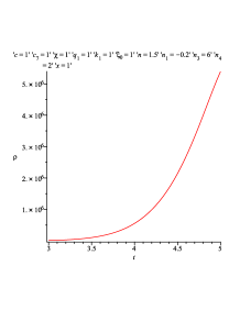
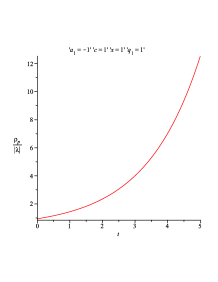
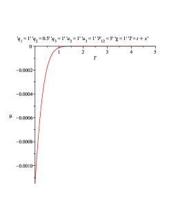
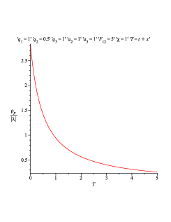
The expressions for energy density ρ𝜌\rho, the string tension density λ𝜆\lambda, magnetic permeability μ¯¯𝜇\bar{\mu} and The particle density ρpsubscript𝜌𝑝\rho_{p}, for the model (61), are given by:

ρ(x,t)=λ(x,t)=n1exp[2c7(n(x+t)x)]secn1[ξ](n3cos[ξ]n4sin[ξ]),𝜌𝑥𝑡𝜆𝑥𝑡subscript𝑛12subscript𝑐7𝑛𝑥𝑡𝑥superscriptsubscript𝑛1𝜉subscript𝑛3𝜉subscript𝑛4𝜉missing-subexpression\begin{array}[]{ll}\rho(x,t)=-\lambda(x,t)=n_{1}\,\exp\Big{[}2\,c_{7}\Big{(}n\,(x+t)-x\Big{)}\Big{]}\,\sec^{n_{1}}\big{[}\xi\big{]}\,\Big{(}n_{3}\,\cos\big{[}\xi\big{]}-n_{4}\,\sin\big{[}\xi\big{]}\Big{)},\end{array} (75)
μ¯(x,t)=χF122(x)exp[c(txn1(x+t))]2cn1q22cos2n1[ξ](2K1tan[ξ]c7),¯𝜇𝑥𝑡𝜒subscriptsuperscript𝐹212𝑥𝑐𝑡𝑥subscript𝑛1𝑥𝑡2𝑐subscript𝑛1superscriptsubscript𝑞22superscript2subscript𝑛1𝜉2subscript𝐾1𝜉subscript𝑐7missing-subexpression\begin{array}[]{ll}\bar{\mu}(x,t)\,=\dfrac{\chi\,F^{2}_{12}(x)\,\exp\Big{[}c\,\Big{(}t-x-n_{1}\,(x+t)\Big{)}\Big{]}}{2\,c\,n_{1}\,q_{2}^{2}\,\cos^{2\,n_{1}}\big{[}\xi\big{]}\,\Big{(}2\,K_{1}\,\tan\big{[}\xi\big{]}-c_{7}\Big{)}},\end{array} (76)
ρp(x,t)=n5exp[2c7(n(x+t)x)]cosn[ξ],subscript𝜌𝑝𝑥𝑡subscript𝑛52subscript𝑐7𝑛𝑥𝑡𝑥superscript𝑛𝜉missing-subexpression\begin{array}[]{ll}\rho_{p}(x,t)\,=n_{5}\,\exp\Big{[}2\,c_{7}\Big{(}n\,(x+t)-x\Big{)}\Big{]}\,\cos^{n}\big{[}\xi\big{]},\end{array} (77)

where n3=c7(c+c7)+4K12χq12subscript𝑛3subscript𝑐7𝑐subscript𝑐74superscriptsubscript𝐾12𝜒superscriptsubscript𝑞12n_{3}=\dfrac{c_{7}\,(c+c_{7})+4\,K_{1}^{2}}{\chi\,q_{1}^{2}}, n4=2cK1χq12subscript𝑛42𝑐subscript𝐾1𝜒superscriptsubscript𝑞12n_{4}=\dfrac{2\,c\,K_{1}}{\chi\,q_{1}^{2}}, n5=2c2q12subscript𝑛52superscript𝑐2superscriptsubscript𝑞12n_{5}=\dfrac{2\,c^{2}}{q_{1}^{2}}, ξ=K1(x+t)+ξ0𝜉subscript𝐾1𝑥𝑡subscript𝜉0\xi=K_{1}\,\big{(}x+t\big{)}+\xi_{0} and F12(x)subscript𝐹12𝑥F_{12}(x) is an arbitrary function of the variable x𝑥x.

The volume element is

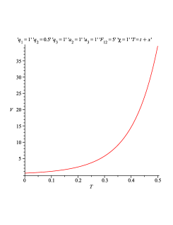
V=q12q2q3exp[c72(3xt+3n1(x+t))]cos3n11[ξ].𝑉superscriptsubscript𝑞12subscript𝑞2subscript𝑞3subscript𝑐723𝑥𝑡3subscript𝑛1𝑥𝑡superscript3subscript𝑛11𝜉V=q_{1}^{2}\,q_{2}\,q_{3}\,\exp\Big{[}\dfrac{c_{7}}{2}\Big{(}3\,x-t+3\,n_{1}\,(x+t)\Big{)}\Big{]}\,\cos^{3\,n_{1}-1}\big{[}\xi\big{]}. (78)

The expansion scalar, which determines the volume behavior of the fluid, is given by:

Θ=(5n114q1)(c7cos[ξ]2K1sin[ξ])exp[c7(n(x+t)x)]secnn11[ξ],Θ5subscript𝑛114subscript𝑞1subscript𝑐7𝜉2subscript𝐾1𝜉subscript𝑐7𝑛𝑥𝑡𝑥superscript𝑛subscript𝑛11𝜉missing-subexpression\begin{array}[]{ll}\Theta=\Big{(}\dfrac{5\,n_{1}-1}{4\,q_{1}}\Big{)}\,\Big{(}c_{7}\,\cos\big{[}\xi\big{]}-2\,K_{1}\,\sin\big{[}\xi\big{]}\Big{)}\,\exp\Big{[}c_{7}\Big{(}n\,(x+t)-x\Big{)}\Big{]}\,\sec^{n\,n_{1}-1}\big{[}\xi\big{]},\end{array} (79)

The non-vanishing components of the shear tensor, σijsuperscriptsubscript𝜎𝑖𝑗\sigma_{i}^{j}, are:

σ11=2(n1+1)Θ3(15n1).superscriptsubscript𝜎112subscript𝑛11Θ315subscript𝑛1missing-subexpression\begin{array}[]{ll}\sigma_{1}^{1}\,=\dfrac{2\,(n_{1}+1)\,\Theta}{3\,(1-5\,n_{1})}.\end{array} (80)
σ22=Θ3(5n11)[n1+16ccos[ξ]c7cos[ξ]2K1sin[ξ]],superscriptsubscript𝜎22Θ35subscript𝑛11delimited-[]subscript𝑛116𝑐𝜉subscript𝑐7𝜉2subscript𝐾1𝜉missing-subexpression\begin{array}[]{ll}\sigma_{2}^{2}\,=\dfrac{\Theta}{3\,(5\,n_{1}-1)}\Big{[}n_{1}+1-\dfrac{6\,c\,\cos\big{[}\xi\big{]}}{c_{7}\,\cos\big{[}\xi\big{]}-2\,K_{1}\,\sin\big{[}\xi\big{]}}\Big{]},\end{array} (81)
σ33=(σ11+σ22).superscriptsubscript𝜎33superscriptsubscript𝜎11superscriptsubscript𝜎22missing-subexpression\begin{array}[]{ll}\sigma_{3}^{3}\,=-\Big{(}\sigma_{1}^{1}+\sigma_{2}^{2}\Big{)}.\end{array} (82)

The shear scalar is:

σ2=[n6+n7cos[ξ]4c7K1sin[ξ]]Θ26(15n1)2(c7cos[ξ]2K1sin[ξ])2,superscript𝜎2delimited-[]subscript𝑛6subscript𝑛7𝜉4subscript𝑐7subscript𝐾1𝜉superscriptΘ26superscript15subscript𝑛12superscriptsubscript𝑐7𝜉2subscript𝐾1𝜉2missing-subexpression\begin{array}[]{ll}\sigma^{2}\,=\dfrac{\Big{[}n_{6}+n_{7}\,\cos\big{[}\xi\big{]}-4\,c_{7}\,K_{1}\,\sin\big{[}\xi\big{]}\Big{]}\,\Theta^{2}}{6\,(1-5\,n_{1})^{2}\,\Big{(}c_{7}\,\cos\big{[}\xi\big{]}-2\,K_{1}\,\sin\big{[}\xi\big{]}\Big{)}^{2}},\end{array} (83)

where n6=(n1210n1+1)(c72+4K12)subscript𝑛6superscriptsubscript𝑛1210subscript𝑛11superscriptsubscript𝑐724superscriptsubscript𝐾12n_{6}=(n_{1}^{2}-10\,n_{1}+1)(c_{7}^{2}+4\,K_{1}^{2}) and n7=(n12+1)(c724K12)2n1(5c72+28K12)subscript𝑛7superscriptsubscript𝑛121superscriptsubscript𝑐724superscriptsubscript𝐾122subscript𝑛15superscriptsubscript𝑐7228superscriptsubscript𝐾12n_{7}=(n_{1}^{2}+1)(c_{7}^{2}-4\,K_{1}^{2})-2\,n_{1}\,(5\,c_{7}^{2}+28\,K_{1}^{2}).

The acceleration vector is given by:

u˙i=14(c7(n1+3)+2K1(1n1)tan[ξ],0,0,0).subscript˙𝑢𝑖14subscript𝑐7subscript𝑛132subscript𝐾11subscript𝑛1𝜉000missing-subexpression\begin{array}[]{ll}\dot{u}_{i}=\dfrac{1}{4}\Big{(}c_{7}\,(n_{1}+3)+2\,K_{1}\,(1-n_{1})\,\tan\big{[}\xi\big{]},0,0,0\Big{)}.\end{array} (84)

The deceleration parameter is given by [18, 19]

𝐪=3Θ2(Θ;iui+13Θ2)=(5n11)3256q14exp[4c7(n(x+t)x)](c7cos[ξ]2K1sin[ξ])×(c2c72+20K11(n1+1)[(c724K12)cos[ξ]4c7K1sin[ξ]]).\begin{array}[]{ll}\mathbf{q}&=-3\,\Theta^{2}\,\Big{(}\Theta_{;i}\,u^{i}+\dfrac{1}{3}\,\Theta^{2}\Big{)}\\ &=\dfrac{(5\,n_{1}-1)^{3}}{256\,q_{1}^{4}}\exp\Big{[}4\,c_{7}\Big{(}n\,(x+t)-x\Big{)}\Big{]}\,\Big{(}c_{7}\,\cos\big{[}\xi\big{]}-2\,K_{1}\,\sin\big{[}\xi\big{]}\Big{)}\\ &\,\,\,\,\,\times\Bigg{(}c^{2}-c_{7}^{2}+20\,K_{1}^{1}-(n_{1}+1)\Big{[}(c_{7}^{2}-4\,K_{1}^{2})\,\cos\big{[}\xi\big{]}-4\,c_{7}\,K_{1}\,\sin\big{[}\xi\big{]}\Big{]}\Bigg{)}.\end{array} (85)

Remark (3): It is worth noting that: If we put the following transformation

K1ıK2,sinsinh,coscosh,formulae-sequencesubscript𝐾1italic-ısubscript𝐾2formulae-sequenceK_{1}\,\rightarrow\,\imath\,K_{2},\,\,\,\sin\,\rightarrow\,\sinh,\,\,\,\cos\,\rightarrow\,\cosh,

in the model (61), we have obtained the model (63), where ı=1italic-ı1\imath=\sqrt{-1}. Therefore, we can find the physical properties of the model correspondence to case (1.1.2) by putting the above transformation in the the model correspondence to case (1.1.1).

For the Model (65):

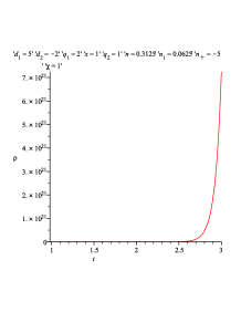
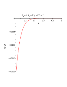
The expressions for energy density ρ𝜌\rho, the string tension density λ𝜆\lambda, magnetic permeability μ¯¯𝜇\bar{\mu} and The particle density ρpsubscript𝜌𝑝\rho_{p}, for the model (65), are given by:

ρ(x,t)=λ(x,t)=4d1χq12(x+t)d22[d22n+(x+t)]exp[4d1d2(nt+n1x)],𝜌𝑥𝑡𝜆𝑥𝑡4subscript𝑑1𝜒superscriptsubscript𝑞12superscript𝑥𝑡superscriptsubscript𝑑22delimited-[]superscriptsubscript𝑑22subscript𝑛𝑥𝑡4subscript𝑑1subscript𝑑2𝑛𝑡subscript𝑛1𝑥missing-subexpression\begin{array}[]{ll}\rho(x,t)=-\lambda(x,t)=\dfrac{4\,d_{1}}{\chi\,q_{1}^{2}}\,(x+t)^{d_{2}^{2}}\,\Big{[}d_{2}^{2}-n_{+}\,(x+t)\Big{]}\,\exp\Big{[}-4\,d_{1}\,d_{2}\,(n\,t+n_{1}\,x)\Big{]},\end{array} (86)
μ¯(x,t)=χF122(x)(x+t)1+2d22exp[4(n+t+nx)]8d1d2q22[d1(x+t)d2],¯𝜇𝑥𝑡𝜒subscriptsuperscript𝐹212𝑥superscript𝑥𝑡12superscriptsubscript𝑑224subscript𝑛𝑡subscript𝑛𝑥8subscript𝑑1subscript𝑑2superscriptsubscript𝑞22delimited-[]subscript𝑑1𝑥𝑡subscript𝑑2missing-subexpression\begin{array}[]{ll}\bar{\mu}(x,t)\,=\dfrac{\chi\,F^{2}_{12}(x)\,(x+t)^{1+2\,d_{2}^{2}}\,\,\exp\Big{[}-4\,(n_{+}\,t+n_{-}\,x)\Big{]}}{8\,d_{1}\,d_{2}\,q_{2}^{2}\,\Big{[}d_{1}\,(x+t)-d_{2}\Big{]}},\end{array} (87)
ρp(x,t)=8d12q12(x+t)1+d22exp[4d1d2(nt+n1x)],subscript𝜌𝑝𝑥𝑡8superscriptsubscript𝑑12superscriptsubscript𝑞12superscript𝑥𝑡1superscriptsubscript𝑑224subscript𝑑1subscript𝑑2𝑛𝑡subscript𝑛1𝑥missing-subexpression\begin{array}[]{ll}\rho_{p}(x,t)\,=\dfrac{8\,d_{1}^{2}}{q_{1}^{2}}\,(x+t)^{1+d_{2}^{2}}\,\exp\Big{[}-4\,d_{1}\,d_{2}\,(n\,t+n_{1}\,x)\Big{]},\end{array} (88)

where F12(x)subscript𝐹12𝑥F_{12}(x) is an arbitrary function of the variable x𝑥x.

The volume element is

V=q12q2q3(x+t)13d22exp[d1((1+3d22)t+3(d221)x)].𝑉superscriptsubscript𝑞12subscript𝑞2subscript𝑞3superscript𝑥𝑡13superscriptsubscript𝑑22subscript𝑑113superscriptsubscript𝑑22𝑡3superscriptsubscript𝑑221𝑥V=q_{1}^{2}\,q_{2}\,q_{3}\,(x+t)^{-1-3\,d_{2}^{2}}\,\exp\Big{[}d_{1}\,\Big{(}(1+3\,d_{2}^{2})\,t+3\,(d_{2}^{2}-1)\,x\Big{)}\Big{]}. (89)

The expansion scalar, which determines the volume behavior of the fluid, is given by:

Θ=(5d22+1)[d1(x+t)d2]2d2q1(x+t)d2212exp[2d1d2(nt+n1x)],Θ5superscriptsubscript𝑑221delimited-[]subscript𝑑1𝑥𝑡subscript𝑑22subscript𝑑2subscript𝑞1superscript𝑥𝑡superscriptsubscript𝑑22122subscript𝑑1subscript𝑑2𝑛𝑡subscript𝑛1𝑥missing-subexpression\begin{array}[]{ll}\Theta=\dfrac{(5\,d_{2}^{2}+1)\,\Big{[}d_{1}\,(x+t)-d_{2}\Big{]}}{2\,d_{2}\,q_{1}}\,(x+t)^{\dfrac{d_{2}^{2}-1}{2}}\,\exp\Big{[}-2\,d_{1}\,d_{2}\,(n\,t+n_{1}\,x)\Big{]},\end{array} (90)

The non-vanishing components of the shear tensor, σijsuperscriptsubscript𝜎𝑖𝑗\sigma_{i}^{j}, are:

σ11=2(1d22)Θ3(15d22).superscriptsubscript𝜎1121superscriptsubscript𝑑22Θ315superscriptsubscript𝑑22missing-subexpression\begin{array}[]{ll}\sigma_{1}^{1}\,=\dfrac{2\,(1-d_{2}^{2})\,\Theta}{3\,(1-5\,d_{2}^{2})}.\end{array} (91)
σ22=[d2(1+d2)+d1(16d2d22)(x+t)]Θ3(1+5d22)[d2d1(x+t)],superscriptsubscript𝜎22delimited-[]subscript𝑑21subscript𝑑2subscript𝑑116subscript𝑑2superscriptsubscript𝑑22𝑥𝑡Θ315superscriptsubscript𝑑22delimited-[]subscript𝑑2subscript𝑑1𝑥𝑡missing-subexpression\begin{array}[]{ll}\sigma_{2}^{2}\,=\dfrac{\Big{[}d_{2}\,(1+d_{2})+d_{1}\,(1-6\,d_{2}-d_{2}^{2})\,(x+t)\Big{]}\,\Theta}{3\,(1+5\,d_{2}^{2})\,\Big{[}d_{2}-d_{1}\,(x+t)\Big{]}},\end{array} (92)
σ33=(σ11+σ22).superscriptsubscript𝜎33superscriptsubscript𝜎11superscriptsubscript𝜎22missing-subexpression\begin{array}[]{ll}\sigma_{3}^{3}\,=-\Big{(}\sigma_{1}^{1}+\sigma_{2}^{2}\Big{)}.\end{array} (93)

The shear scalar is:

σ2=Θ23(1+5d22)2[1+d22(10+d22)+12d23(2d1(x+t)2d2+1)(d1(x+t)d2)2].superscript𝜎2superscriptΘ23superscript15superscriptsubscript𝑑222delimited-[]1superscriptsubscript𝑑2210superscriptsubscript𝑑2212superscriptsubscript𝑑232subscript𝑑1𝑥𝑡2subscript𝑑21superscriptsubscript𝑑1𝑥𝑡subscript𝑑22missing-subexpression\begin{array}[]{ll}\sigma^{2}\,=\dfrac{\Theta^{2}}{3\,(1+5\,d_{2}^{2})^{2}}\,\Bigg{[}1+d_{2}^{2}\,(10+d_{2}^{2})+\dfrac{12\,d_{2}^{3}\Big{(}2\,d_{1}\,(x+t)-2\,d_{2}+1\Big{)}}{\Big{(}d_{1}\,(x+t)-\,d_{2}\Big{)}^{2}}\Bigg{]}.\end{array} (94)

The acceleration vector is given by:

u˙i=2(n1d1nd2x+t,0,0,0).subscript˙𝑢𝑖2subscript𝑛1subscript𝑑1𝑛subscript𝑑2𝑥𝑡000missing-subexpression\begin{array}[]{ll}\dot{u}_{i}=2\Big{(}n_{1}\,d_{1}-\dfrac{n\,d_{2}}{x+t},0,0,0\Big{)}.\end{array} (95)

The deceleration parameter is given by:

𝐪=(5d22+1)38d24q14(x+t)2(d221)exp[8d1d2(nt+n1x)]×(d22(d22+2)+d1(d221)(x+t)[d1(x+t)2d2]).𝐪absentsuperscript5superscriptsubscript𝑑22138superscriptsubscript𝑑24superscriptsubscript𝑞14superscript𝑥𝑡2superscriptsubscript𝑑2218subscript𝑑1subscript𝑑2𝑛𝑡subscript𝑛1𝑥missing-subexpressionabsentsuperscriptsubscript𝑑22superscriptsubscript𝑑222subscript𝑑1superscriptsubscript𝑑221𝑥𝑡delimited-[]subscript𝑑1𝑥𝑡2subscript𝑑2\begin{array}[]{ll}\mathbf{q}&=-\dfrac{(5\,d_{2}^{2}+1)^{3}}{8\,d_{2}^{4}\,q_{1}^{4}}\,(x+t)^{2\,(d_{2}^{2}-1)}\,\exp\Big{[}-8\,d_{1}\,d_{2}\,(n\,t+n_{1}\,x)\Big{]}\\ &\,\,\,\,\,\,\,\,\,\,\,\,\,\,\,\times\Bigg{(}d_{2}^{2}\,(d_{2}^{2}+2)+d_{1}\,(d_{2}^{2}-1)\,(x+t)\,\Big{[}d_{1}\,(x+t)-2\,d_{2}\Big{]}\Bigg{)}.\end{array} (96)

For the Model (67):

The expressions for energy density ρ𝜌\rho, the string tension density λ𝜆\lambda, magnetic permeability μ¯¯𝜇\bar{\mu} and the particle density ρpsubscript𝜌𝑝\rho_{p}, for the model (67), are given by:

ρ(x,t)=λ(x,t)=6a1c2e2c(5t+7x)5χq1[a1e3c(x+t)5]5,𝜌𝑥𝑡𝜆𝑥𝑡6subscript𝑎1superscript𝑐2superscripte2𝑐5𝑡7𝑥5𝜒subscript𝑞1superscriptdelimited-[]subscript𝑎1superscripte3𝑐𝑥𝑡55missing-subexpression\begin{array}[]{ll}\rho(x,t)\,=\,-\lambda(x,t)=\dfrac{6\,a_{1}\,c^{2}\,\mathrm{e}^{\dfrac{2\,c\,(5\,t+7\,x)}{5}}}{\chi\,q_{1}}\,\Big{[}a_{1}-\mathrm{e}^{\dfrac{3\,c\,(x+t)}{5}}\Big{]}^{-5},\end{array} (97)
μ¯(x,t)=χF122(x)e2c(3t+2x)2c2q22[a1e3c(x+t)5]9[5a1e3c(x+t)5]1,¯𝜇𝑥𝑡𝜒subscriptsuperscript𝐹212𝑥superscripte2𝑐3𝑡2𝑥2superscript𝑐2superscriptsubscript𝑞22superscriptdelimited-[]subscript𝑎1superscripte3𝑐𝑥𝑡59superscriptdelimited-[]5subscript𝑎1superscripte3𝑐𝑥𝑡51missing-subexpression\begin{array}[]{ll}\bar{\mu}(x,t)\,=\,\dfrac{\chi\,F^{2}_{12}(x)\,\mathrm{e}^{2\,c\,(3\,t+2\,x)}}{2\,c^{2}\,q_{2}^{2}}\,\Big{[}a_{1}-\mathrm{e}^{\dfrac{3\,c\,(x+t)}{5}}\Big{]}^{-9}\,\Big{[}5\,a_{1}-\mathrm{e}^{\dfrac{3\,c\,(x+t)}{5}}\Big{]}^{-1},\end{array} (98)
ρp(x,t)=2ce2c(5t+7x)5q12[a1e3c(x+t)5]4,subscript𝜌𝑝𝑥𝑡2𝑐superscripte2𝑐5𝑡7𝑥5superscriptsubscript𝑞12superscriptdelimited-[]subscript𝑎1superscripte3𝑐𝑥𝑡54missing-subexpression\begin{array}[]{ll}\rho_{p}(x,t)\,=\,\dfrac{2\,c\,\mathrm{e}^{\dfrac{2\,c\,(5\,t+7\,x)}{5}}}{q_{1}^{2}}\,\Big{[}a_{1}-\mathrm{e}^{\dfrac{3\,c\,(x+t)}{5}}\Big{]}^{-4},\end{array} (99)

where F12(x)subscript𝐹12𝑥F_{12}(x) is an arbitrary function of the variable x𝑥x.

The volume element is

V=q12q2q3ec(35t+39x)5[a1e3c(x+t)5]14.𝑉superscriptsubscript𝑞12subscript𝑞2subscript𝑞3superscripte𝑐35𝑡39𝑥5superscriptdelimited-[]subscript𝑎1superscripte3𝑐𝑥𝑡514V=q_{1}^{2}\,q_{2}\,q_{3}\,\,\mathrm{e}^{\dfrac{-\,c\,(35\,t+39\,x)}{5}}\,\Big{[}a_{1}-\mathrm{e}^{\dfrac{3\,c\,(x+t)}{5}}\Big{]}^{14}. (100)

The expansion scalar, which determines the volume behavior of the fluid, is given by:

Θ=6c5q1ec(5t+7x)5[5a1+e3c(x+t)5][a1e3c(x+t)5]3,Θ6𝑐5subscript𝑞1superscripte𝑐5𝑡7𝑥5delimited-[]5subscript𝑎1superscripte3𝑐𝑥𝑡5superscriptdelimited-[]subscript𝑎1superscripte3𝑐𝑥𝑡53missing-subexpression\begin{array}[]{ll}\Theta=-\dfrac{6\,c}{5\,q_{1}}\,\mathrm{e}^{\dfrac{c\,(5\,t+7\,x)}{5}}\,\Big{[}5\,a_{1}+\mathrm{e}^{\dfrac{3\,c\,(x+t)}{5}}\Big{]}\,\Big{[}a_{1}-\mathrm{e}^{\dfrac{3\,c\,(x+t)}{5}}\Big{]}^{-3},\end{array} (101)

The non-vanishing components of the shear tensor, σijsuperscriptsubscript𝜎𝑖𝑗\sigma_{i}^{j}, are:

σ11=Θ6,superscriptsubscript𝜎11Θ6missing-subexpression\begin{array}[]{ll}\sigma_{1}^{1}\,=\dfrac{\Theta}{6},\end{array} (102)
σ22=Θ6[5a12e3c(x+t)5][5a1+e3c(x+t)5]1,superscriptsubscript𝜎22Θ6delimited-[]5subscript𝑎12superscripte3𝑐𝑥𝑡5superscriptdelimited-[]5subscript𝑎1superscripte3𝑐𝑥𝑡51missing-subexpression\begin{array}[]{ll}\sigma_{2}^{2}\,=\dfrac{\Theta}{6}\,\Big{[}5\,a_{1}-2\,\mathrm{e}^{\dfrac{3\,c\,(x+t)}{5}}\Big{]}\,\Big{[}5\,a_{1}+\mathrm{e}^{\dfrac{3\,c\,(x+t)}{5}}\Big{]}^{-1},\end{array} (103)
σ33=(σ11+σ22).superscriptsubscript𝜎33superscriptsubscript𝜎11superscriptsubscript𝜎22missing-subexpression\begin{array}[]{ll}\sigma_{3}^{3}\,=-\Big{(}\sigma_{1}^{1}+\sigma_{2}^{2}\Big{)}.\end{array} (104)

The shear scalar is:

σ2=Θ236[25a125a1e3c(x+t)5+7e6c(x+t)5][5a1+e3c(x+t)5]2.superscript𝜎2superscriptΘ236delimited-[]25superscriptsubscript𝑎125subscript𝑎1superscripte3𝑐𝑥𝑡57superscripte6𝑐𝑥𝑡5superscriptdelimited-[]5subscript𝑎1superscripte3𝑐𝑥𝑡52missing-subexpression\begin{array}[]{ll}\sigma^{2}\,=\dfrac{\Theta^{2}}{36}\,\Big{[}25\,a_{1}^{2}-5\,a_{1}\,\mathrm{e}^{\dfrac{3\,c\,(x+t)}{5}}+7\,\mathrm{e}^{\dfrac{6\,c\,(x+t)}{5}}\Big{]}\,\Big{[}5\,a_{1}+\mathrm{e}^{\dfrac{3\,c\,(x+t)}{5}}\Big{]}^{-2}.\end{array} (105)

The acceleration vector is given by:

u˙i=c7[7a1e3c(x+t)5][a1e3c(x+t)5]1(1,0,0,0).subscript˙𝑢𝑖𝑐7delimited-[]7subscript𝑎1superscripte3𝑐𝑥𝑡5superscriptdelimited-[]subscript𝑎1superscripte3𝑐𝑥𝑡511000missing-subexpression\begin{array}[]{ll}\dot{u}_{i}=-\dfrac{c}{7}\Big{[}7\,a_{1}-\mathrm{e}^{\dfrac{3\,c\,(x+t)}{5}}\Big{]}\,\Big{[}a_{1}-\mathrm{e}^{\dfrac{3\,c\,(x+t)}{5}}\Big{]}^{-1}\,\Big{(}1,0,0,0\Big{)}.\end{array} (106)

The deceleration parameter is given by:

𝐪=18c2Θ225q12e2c(5t+7t)5[a1e3c(x+t)5]6×[25a128a1e3c(x+t)5+e6c(x+t)5].𝐪absent18superscript𝑐2superscriptΘ225superscriptsubscript𝑞12superscripte2𝑐5𝑡7𝑡5superscriptdelimited-[]subscript𝑎1superscripte3𝑐𝑥𝑡56missing-subexpressionabsentdelimited-[]25superscriptsubscript𝑎128subscript𝑎1superscripte3𝑐𝑥𝑡5superscripte6𝑐𝑥𝑡5\begin{array}[]{ll}\mathbf{q}&=-\dfrac{18\,c^{2}\,\Theta^{2}}{25\,q_{1}^{2}}\,\mathrm{e}^{\dfrac{2\,c\,(5\,t+7\,t)}{5}}\,\Big{[}a_{1}-\mathrm{e}^{\dfrac{3\,c\,(x+t)}{5}}\Big{]}^{-6}\\ &\,\,\,\,\,\,\,\,\,\,\,\,\,\,\,\,\,\,\,\,\times\Big{[}25\,a_{1}^{2}-8\,a_{1}\,\mathrm{e}^{\dfrac{3\,c\,(x+t)}{5}}+\,\mathrm{e}^{\dfrac{6\,c\,(x+t)}{5}}\Big{]}.\end{array} (107)

For the Model (69):

The expressions for energy density ρ𝜌\rho, the string tension density λ𝜆\lambda, magnetic permeability μ¯¯𝜇\bar{\mu} and the particle density ρpsubscript𝜌𝑝\rho_{p}, for the model (69), are given by:

ρ(x,t)=λ(x,t)=4b1χb2q12[b1(b1+b2)b2eb2(x+t)]×exp[12b2(b12(x+t)2b22eb2(x+t))],𝜌𝑥𝑡𝜆𝑥𝑡4subscript𝑏1𝜒subscript𝑏2superscriptsubscript𝑞12delimited-[]subscript𝑏1subscript𝑏1subscript𝑏2subscript𝑏2superscriptesubscript𝑏2𝑥𝑡missing-subexpressionmissing-subexpressionmissing-subexpressionabsent12subscript𝑏2superscriptsubscript𝑏12𝑥𝑡2superscriptsubscript𝑏22superscriptesubscript𝑏2𝑥𝑡missing-subexpression\begin{array}[]{ll}\rho(x,t)\,=\,-\lambda(x,t)=-\dfrac{4\,b_{1}}{\chi\,b_{2}\,q_{1}^{2}}\,\Big{[}b_{1}\,(b_{1}+b_{2})-b_{2}\,\mathrm{e}^{b_{2}\,(x+t)}\Big{]}\\ \\ \,\,\,\,\,\,\,\,\,\,\,\,\,\,\,\,\,\,\,\,\,\,\,\,\,\,\,\,\,\,\,\,\,\,\,\,\,\,\,\,\,\,\times\exp\Big{[}\dfrac{1}{2\,b_{2}}\,\Big{(}b_{1}^{2}\,(x+t)-2\,b_{2}^{2}-\mathrm{e}^{b_{2}\,(x+t)}\Big{)}\Big{]},\end{array} (108)
μ¯(x,t)=χb2F122(x)8b1q22[b1b2eb2(x+t)]exp[2b2[b1(b2(tx)+b1(x+t))eb2(x+t)]],¯𝜇𝑥𝑡𝜒subscript𝑏2subscriptsuperscript𝐹212𝑥8subscript𝑏1superscriptsubscript𝑞22delimited-[]subscript𝑏1subscript𝑏2superscriptesubscript𝑏2𝑥𝑡2subscript𝑏2delimited-[]subscript𝑏1subscript𝑏2𝑡𝑥subscript𝑏1𝑥𝑡superscriptesubscript𝑏2𝑥𝑡missing-subexpression\begin{array}[]{ll}\bar{\mu}(x,t)=\dfrac{\chi\,b_{2}\,F^{2}_{12}(x)}{8\,b_{1}\,q_{2}^{2}\,\Big{[}b_{1}-b_{2}\,\mathrm{e}^{b_{2}\,(x+t)}\Big{]}}\,\exp\Big{[}\dfrac{2}{b_{2}}\,\Big{[}b_{1}\Big{(}b_{2}\,(t-x)+b_{1}\,(x+t)\Big{)}-\mathrm{e}^{b_{2}\,(x+t)}\Big{]}\Big{]},\end{array} (109)
ρp(x,t)=8b12q12exp[1b2(b12(xt)2b22xeb2(x+t))],subscript𝜌𝑝𝑥𝑡8superscriptsubscript𝑏12superscriptsubscript𝑞121subscript𝑏2superscriptsubscript𝑏12𝑥𝑡2superscriptsubscript𝑏22𝑥superscriptesubscript𝑏2𝑥𝑡missing-subexpression\begin{array}[]{ll}\rho_{p}(x,t)\,=\,\dfrac{8\,b_{1}^{2}}{q_{1}^{2}}\,\exp\Big{[}\dfrac{1}{b_{2}}\,\Big{(}b_{1}^{2}(x-t)-2\,b_{2}^{2}\,x-\mathrm{e}^{b_{2}\,(x+t)}\Big{)}\Big{]},\end{array} (110)

where F12(x)subscript𝐹12𝑥F_{12}(x) is an arbitrary function of the variable x𝑥x.

The volume element is

V=q12q2q3exp[1b2(2b22x3b12(xt)+3eb2(x+t))].𝑉superscriptsubscript𝑞12subscript𝑞2subscript𝑞31subscript𝑏22superscriptsubscript𝑏22𝑥3superscriptsubscript𝑏12𝑥𝑡3superscriptesubscript𝑏2𝑥𝑡V=q_{1}^{2}\,q_{2}\,q_{3}\,\exp\Big{[}\dfrac{1}{b_{2}}\,\Big{(}2\,b_{2}^{2}\,x-3\,b_{1}^{2}(x-t)+3\,\mathrm{e}^{b_{2}\,(x+t)}\Big{)}\Big{]}. (111)

The expansion scalar, which determines the volume behavior of the fluid, is given by:

Θ=52b2q1[b2eb2(x+t)b12]exp[12b2(b12(x+t)2b22xeb2(x+t))],,Θ52subscript𝑏2subscript𝑞1delimited-[]subscript𝑏2superscriptesubscript𝑏2𝑥𝑡superscriptsubscript𝑏1212subscript𝑏2superscriptsubscript𝑏12𝑥𝑡2superscriptsubscript𝑏22𝑥superscriptesubscript𝑏2𝑥𝑡missing-subexpression\begin{array}[]{ll}\Theta=\,\dfrac{5}{2\,b_{2}\,q_{1}}\,\Big{[}b_{2}\,\mathrm{e}^{b_{2}\,(x+t)}-b_{1}^{2}\Big{]}\,\exp\Big{[}\dfrac{1}{2\,b_{2}}\,\Big{(}b_{1}^{2}\,(x+t)-2\,b_{2}^{2}\,x-\mathrm{e}^{b_{2}\,(x+t)}\Big{)}\Big{]},,\end{array} (112)

The non-vanishing components of the shear tensor, σijsuperscriptsubscript𝜎𝑖𝑗\sigma_{i}^{j}, are:

σ11=2Θ15,superscriptsubscript𝜎112Θ15missing-subexpression\begin{array}[]{ll}\sigma_{1}^{1}\,=-\dfrac{2\,\Theta}{15},\end{array} (113)
σ22=Θ15(b12+6b1b2b2eb2(x+t)b12b2eb2(x+t)),superscriptsubscript𝜎22Θ15superscriptsubscript𝑏126subscript𝑏1subscript𝑏2subscript𝑏2superscriptesubscript𝑏2𝑥𝑡superscriptsubscript𝑏12subscript𝑏2superscriptesubscript𝑏2𝑥𝑡missing-subexpression\begin{array}[]{ll}\sigma_{2}^{2}\,=\dfrac{\Theta}{15}\,\Big{(}\dfrac{b_{1}^{2}+6\,b_{1}\,b_{2}-b_{2}\,\mathrm{e}^{b_{2}\,(x+t)}}{b_{1}^{2}-b_{2}\,\mathrm{e}^{b_{2}\,(x+t)}}\Big{)},\end{array} (114)
σ33=(σ11+σ22).superscriptsubscript𝜎33superscriptsubscript𝜎11superscriptsubscript𝜎22missing-subexpression\begin{array}[]{ll}\sigma_{3}^{3}\,=-\Big{(}\sigma_{1}^{1}+\sigma_{2}^{2}\Big{)}.\end{array} (115)

The shear scalar is:

σ2=Θ225[13+4b12b22(b12b2eb2(x+t))2].superscript𝜎2superscriptΘ225delimited-[]134superscriptsubscript𝑏12superscriptsubscript𝑏22superscriptsuperscriptsubscript𝑏12subscript𝑏2superscriptesubscript𝑏2𝑥𝑡2missing-subexpression\begin{array}[]{ll}\sigma^{2}\,=\dfrac{\Theta^{2}}{25}\,\Big{[}\dfrac{1}{3}+4\,b_{1}^{2}\,b_{2}^{2}\,\Big{(}b_{1}^{2}-b_{2}\,\mathrm{e}^{b_{2}\,(x+t)}\Big{)}^{-2}\Big{]}.\end{array} (116)

The acceleration vector is given by:

u˙i=12d1[2b22b12+b2eb2(x+t)](1,0,0,0).subscript˙𝑢𝑖12subscript𝑑1delimited-[]2superscriptsubscript𝑏22superscriptsubscript𝑏12subscript𝑏2superscriptesubscript𝑏2𝑥𝑡1000missing-subexpression\begin{array}[]{ll}\dot{u}_{i}=\dfrac{1}{2\,d_{1}}\Big{[}2\,b_{2}^{2}-b_{1}^{2}+b_{2}\,\mathrm{e}^{b_{2}\,(x+t)}\Big{]}\,\Big{(}1,0,0,0\Big{)}.\end{array} (117)

The deceleration parameter is given by:

𝐪=5Θ22b22q12[b12+b2(3b222b12)eb22(x+t)+2b22eb2(x+t)]×exp[1b2(2b22b12(x+t)+eb2(x+t))].𝐪5superscriptΘ22superscriptsubscript𝑏22superscriptsubscript𝑞12delimited-[]superscriptsubscript𝑏12subscript𝑏23superscriptsubscript𝑏222superscriptsubscript𝑏12superscriptesuperscriptsubscript𝑏22𝑥𝑡2superscriptsubscript𝑏22superscriptesubscript𝑏2𝑥𝑡missing-subexpressionmissing-subexpressionmissing-subexpressionabsent1subscript𝑏22superscriptsubscript𝑏22superscriptsubscript𝑏12𝑥𝑡superscriptesubscript𝑏2𝑥𝑡missing-subexpression\begin{array}[]{ll}\mathbf{q}=-\dfrac{5\,\Theta^{2}}{2\,b_{2}^{2}\,q_{1}^{2}}\,\Big{[}b_{1}^{2}+b_{2}\,(3\,b_{2}^{2}-2\,b_{1}^{2})\,\mathrm{e}^{b_{2}^{2}\,(x+t)}+2\,b_{2}^{2}\,\mathrm{e}^{b_{2}\,(x+t)}\Big{]}\\ \\ \,\,\,\,\,\,\,\,\,\,\,\,\,\,\,\,\,\,\,\,\,\,\,\,\,\,\,\,\,\,\,\,\times\exp\Big{[}-\dfrac{1}{b_{2}}\,\Big{(}2\,b_{2}^{2}-b_{1}^{2}\,(x+t)+\mathrm{e}^{b_{2}\,(x+t)}\Big{)}\Big{]}.\end{array} (118)

For the Model (71):

The expressions for energy density ρ𝜌\rho, the string tension density λ𝜆\lambda, magnetic permeability μ¯¯𝜇\bar{\mu} and the particle density ρpsubscript𝜌𝑝\rho_{p}, for the model (71), are given by:

ρ(x,t)=λ(x,t)=42a3χq12[a2+2a32(x+t)]exp[(x+t)(a2+2a3+a32(x+t))],𝜌𝑥𝑡𝜆𝑥𝑡42subscript𝑎3𝜒superscriptsubscript𝑞12delimited-[]subscript𝑎22superscriptsubscript𝑎32𝑥𝑡𝑥𝑡subscript𝑎22subscript𝑎3superscriptsubscript𝑎32𝑥𝑡missing-subexpression\begin{array}[]{ll}\rho(x,t)\,=\,-\lambda(x,t)=\dfrac{4\,\sqrt{2}\,a_{3}}{\chi\,q_{1}^{2}}\,\Big{[}a_{2}+2\,a_{3}^{2}\,(x+t)\Big{]}\,\exp\Big{[}-(x+t)\Big{(}a_{2}+\sqrt{2}\,a_{3}+a_{3}^{2}\,(x+t)\Big{)}\Big{]},\end{array} (119)
μ¯(x,t)=χF122(x)82a3q22[2a3+a2+2a22(x+t)]1×exp[2(22a3+a2(x+t)+a32(x+t)2)],¯𝜇𝑥𝑡𝜒subscriptsuperscript𝐹212𝑥82subscript𝑎3superscriptsubscript𝑞22superscriptdelimited-[]2subscript𝑎3subscript𝑎22superscriptsubscript𝑎22𝑥𝑡1missing-subexpressionmissing-subexpressionmissing-subexpressionabsent222subscript𝑎3subscript𝑎2𝑥𝑡superscriptsubscript𝑎32superscript𝑥𝑡2missing-subexpression\begin{array}[]{ll}\bar{\mu}(x,t)\,=\,-\dfrac{\chi\,F^{2}_{12}(x)}{8\,\sqrt{2}\,a_{3}\,q_{2}^{2}}\,\Big{[}\sqrt{2}\,a_{3}+a_{2}+2\,a_{2}^{2}\,(x+t)\Big{]}^{-1}\\ \\ \,\,\,\,\,\,\,\,\,\,\times\exp\Big{[}-2\Big{(}2\,\sqrt{2}\,a_{3}+a_{2}\,(x+t)+a_{3}^{2}\,(x+t)^{2}\Big{)}\Big{]},\end{array} (120)
ρp(x,t)=16a32q12exp[(x+t)(2a3+a2+a32(x+t))],subscript𝜌𝑝𝑥𝑡16superscriptsubscript𝑎32superscriptsubscript𝑞12𝑥𝑡2subscript𝑎3subscript𝑎2superscriptsubscript𝑎32𝑥𝑡missing-subexpression\begin{array}[]{ll}\rho_{p}(x,t)\,=\,\dfrac{16\,a_{3}^{2}}{q_{1}^{2}}\,\exp\Big{[}-(x+t)\,\Big{(}\sqrt{2}\,a_{3}+a_{2}+a_{3}^{2}\,(x+t)\Big{)}\Big{]},\end{array} (121)

where F12(x)subscript𝐹12𝑥F_{12}(x) is an arbitrary function of the variable x𝑥x.

The volume element is

V=q12q2q3exp[3(x+t)(2a3+a2+a32(x+t))].𝑉superscriptsubscript𝑞12subscript𝑞2subscript𝑞33𝑥𝑡2subscript𝑎3subscript𝑎2superscriptsubscript𝑎32𝑥𝑡V=q_{1}^{2}\,q_{2}\,q_{3}\,\exp\Big{[}3(x+t)\,\Big{(}\sqrt{2}\,a_{3}+a_{2}+a_{3}^{2}\,(x+t)\Big{)}\Big{]}. (122)

The expansion scalar, which determines the volume behavior of the fluid, is given by:

Θ=52q1[2a3+a2+2a32(x+t)]exp[(x+t2)(2a3+a2+a32(x+t))],Θ52subscript𝑞1delimited-[]2subscript𝑎3subscript𝑎22superscriptsubscript𝑎32𝑥𝑡𝑥𝑡22subscript𝑎3subscript𝑎2superscriptsubscript𝑎32𝑥𝑡missing-subexpression\begin{array}[]{ll}\Theta=\,\dfrac{5}{2\,q_{1}}\,\Big{[}\sqrt{2}\,a_{3}+a_{2}+2\,a_{3}^{2}\,(x+t)\Big{]}\,\exp\Big{[}-\Big{(}\dfrac{x+t}{2}\Big{)}\,\Big{(}\sqrt{2}\,a_{3}+a_{2}+a_{3}^{2}\,(x+t)\Big{)}\Big{]},\end{array} (123)

The non-vanishing components of the shear tensor, σijsuperscriptsubscript𝜎𝑖𝑗\sigma_{i}^{j}, are:

σ11=2Θ15,superscriptsubscript𝜎112Θ15missing-subexpression\begin{array}[]{ll}\sigma_{1}^{1}\,=-\dfrac{2\,\Theta}{15},\end{array} (124)
σ22=Θ15(a252a3+2a32(x+t)a2+2a3+2a32(x+t)),superscriptsubscript𝜎22Θ15subscript𝑎252subscript𝑎32superscriptsubscript𝑎32𝑥𝑡subscript𝑎22subscript𝑎32superscriptsubscript𝑎32𝑥𝑡missing-subexpression\begin{array}[]{ll}\sigma_{2}^{2}\,=\dfrac{\Theta}{15}\,\Big{(}\dfrac{a_{2}-5\,\sqrt{2}\,a_{3}+2\,a_{3}^{2}\,(x+t)}{a_{2}+\sqrt{2}\,a_{3}+2\,a_{3}^{2}\,(x+t)}\Big{)},\end{array} (125)
σ33=(σ11+σ22).superscriptsubscript𝜎33superscriptsubscript𝜎11superscriptsubscript𝜎22missing-subexpression\begin{array}[]{ll}\sigma_{3}^{3}\,=-\Big{(}\sigma_{1}^{1}+\sigma_{2}^{2}\Big{)}.\end{array} (126)

The shear scalar is:

σ2=Θ225[13+8a32(a2+2a3+2a32(x+t))2].superscript𝜎2superscriptΘ225delimited-[]138superscriptsubscript𝑎32superscriptsubscript𝑎22subscript𝑎32superscriptsubscript𝑎32𝑥𝑡2missing-subexpression\begin{array}[]{ll}\sigma^{2}\,=\dfrac{\Theta^{2}}{25}\,\Big{[}\dfrac{1}{3}+8\,a_{3}^{2}\,\Big{(}a_{2}+\sqrt{2}\,a_{3}+2\,a_{3}^{2}\,(x+t)\Big{)}^{-2}\Big{]}.\end{array} (127)

The acceleration vector is given by:

u˙i=[a32+a22+a32(x+t)](1,0,0,0).subscript˙𝑢𝑖delimited-[]subscript𝑎32subscript𝑎22superscriptsubscript𝑎32𝑥𝑡1000missing-subexpression\begin{array}[]{ll}\dot{u}_{i}=\Big{[}\dfrac{a_{3}}{\sqrt{2}}+\dfrac{a_{2}}{2}+a_{3}^{2}\,(x+t)\Big{]}\,\Big{(}1,0,0,0\Big{)}.\end{array} (128)

The deceleration parameter is given by:

𝐪=5Θ22q12[22a3a2+a22+8a32+4a32(2a3+a2)(x+t)+4a34(x+t)2]×exp[(x+t)(a2+2a3+a32(x+t))].𝐪5superscriptΘ22superscriptsubscript𝑞12delimited-[]22subscript𝑎3subscript𝑎2superscriptsubscript𝑎228superscriptsubscript𝑎324superscriptsubscript𝑎322subscript𝑎3subscript𝑎2𝑥𝑡4superscriptsubscript𝑎34superscript𝑥𝑡2missing-subexpressionmissing-subexpressionmissing-subexpressionabsent𝑥𝑡subscript𝑎22subscript𝑎3superscriptsubscript𝑎32𝑥𝑡missing-subexpression\begin{array}[]{ll}\mathbf{q}=-\dfrac{5\,\Theta^{2}}{2\,q_{1}^{2}}\,\Big{[}2\,\sqrt{2}\,a_{3}\,a_{2}+a_{2}^{2}+8\,a_{3}^{2}+4\,a_{3}^{2}\,(\sqrt{2}\,a_{3}+a_{2})\,(x+t)+4\,a_{3}^{4}\,(x+t)^{2}\Big{]}\\ \\ \,\,\,\,\,\,\,\,\,\,\,\,\,\,\,\,\,\,\,\,\,\,\,\,\,\,\,\,\,\,\,\,\times\exp\Big{[}-(x+t)\Big{(}a_{2}+\sqrt{2}\,a_{3}+a_{3}^{2}\,(x+t)\Big{)}\Big{]}.\end{array} (129)

6 Conclusion

In the paper, we have derived some new invariant solutions of Einstein-Maxwell’s field equations for string fluid as source of matter in cylindrically symmetric space-time with Variable Magnetic Permeability. Different set of solutions are found using different values of the parameters. Note that the cosmological solutions are physically viable for the following reasons:

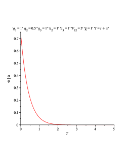
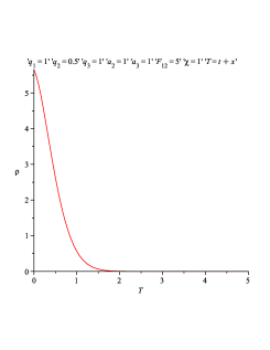
[i] energy density is positive and decreasing with the increase of the time

[ii] volume of the Universe is increasing due the expanding nature of the Universe

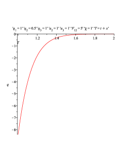
[iii] deceleration parameter should be negative as recent observations indicate that our Universe is accelerating

[iv] σθ𝜎𝜃\frac{\sigma}{\theta} will be vanished at large time as the Universe may got isotropized in some later time

[v] solutions must be non singular as existence of Big-bang singularity is one of the basic failures of general theory of relativity

The models (61), (65), (67) and (69) do not meet the above criterion (i). Here, in the models (61) and (65), densities increase with time whereas in models (67) particle density is increasing and in model (69) particle density is negative (Fig-1). Therefore, these models are not physically interesting. On the other hand, the model (71) is very much acceptable as it describes more or less observable Universe. It is to be noted that our procedure of solving the field equations (symmetry analysis method) is completely different compare to usual methods available in literature. The derived model starts expanding without Big Bang singularity ( fig-2). Also, from the theoretical perspective, the present model can be a viable model to explain the acceleration of the Universe. In other words, the solution presented here can be one of the potential candidates to describe the observed Universe. In our model, it seems magnetic field with negative magnetic Permeability (Fig-3) is responsible to provide accelerated as well as singularity free Universe. Nowadays, negative magnetic permeability is not an impossible event rather it can be found in split ring resonator (SRR) in the visible light region [20]. We also note that σθ𝜎𝜃\frac{\sigma}{\theta} will be vanished at large time (Fig-2). This means the Universe may got isotropized in some later time. Again, one can assume that negative magnetic Permeability is responsible for the isotropisation. A detail discussions of all basic cosmological constraints is beyond the scope in the present paper. We hope it will be taken care in a future project.

Refer to caption Refer to caption Refer to caption Refer to caption
Figure 1: (Left) The variation of energy density with respect to time for the model(61). (First Middle)The variation of energy density with respect to time for the model(65). (Second Middle) The variation of particle density with respect to time for model (67). (Right) The variation of particle density with respect to time for model (69).
Refer to caption Refer to caption Refer to caption
Figure 2: (Left) The variation of the volume of the Universe with respect to time.. (Middle) The variation of σθ𝜎𝜃\frac{\sigma}{\theta} with respect to time. (Right) The deceleration parameter is shown with respect to time.
Refer to caption Refer to caption Refer to caption
Figure 3: (Left) The variation of energy density with respect to time. (Middle) The variation of magnetic Permeability with respect to time. (Right) The variation of particle density with respect to time.

References

  • [1] Barrow JD and Kunze KE, Phys Rev D 56 (1997) 741.
  • [2] Barrow JD and Kunze KE, Phys Rev D 57 (1998) 2255.
  • [3] Pradhan A, Yadav AK, Singh RP and Singh VK, Astrophys Space Science 312 (2007) 145.
  • [4] Yadav AK, Yadav VK and Yadav L, Int J Theor Phys 48 (2009) 568.
  • [5] Attallah SK, El-Sabbagh MF and Ali AT, Commun Nonlinear Sci Numer Simulat 12(7) (2007) 1153.
  • [6] Ali AT, Phys Scr 79(3) (2009) 035006.
  • [7] Mekheimer KS, Husseny SZ, Ali AT and Abo-Elkhair RE, Phys Scr 83(1) (2011) 015017.
  • [8] Ali AT, Phys Scr 87(1) (2013) 015002.
  • [9] Ali AT, Yadav AK and Mahmoud SR, Astrophys Space Science 349(1) (2014) 539.
  • [10] Ovsyannikov LV, ”Group Analysis of Differential Equations”, Academic Press, NY, 1982.
  • [11] Bluman GW and Kumei S, ”Symmetries and differential equations in applied sciences”, New York, 1989.
  • [12] Ibragimov NH, ”Transformation groups applied to mathematical physics”, Reidel, Dordrecht, 1985.
  • [13] Olver PJ, ”Application of Lie Groups to differential equations in graduate texts in mathematics”, Vol. 107, Second edition, Springer, New York, 1993.
  • [14] Melvin MA, Ann N Y Acad Sci 262 (1975) 253.
  • [15] Lichnerowicz A, ”Relativistic Hydrodynamics and Magneto-hydro-dynamics”, W A Benjamin Inc. New-York, p.93, (1967).
  • [16] Synge JL, ”Relativity: The general Theory”, North-Holland Publ. Co., Amesterdam, p.356, 1960.
  • [17] Pradhan A and Mathur P, Fizika B 18 (2009) 243.
  • [18] Feinstein A and lbanez J, Class Quantum Grav 10 (1993) L227.
  • [19] Raychaudhuri AK, ”Theoritical Cosmology”, Oxford, p.80, 1979.
  • [20] Ishikawa A and Tanaka T, Opt Commun 258 (2006) 300.