The Rising Light Curves of Type Ia Supernovae

Abstract

We present an analysis of the early, rising light curves of 18 Type Ia supernovae (SNe Ia) discovered by the Palomar Transient Factory (PTF) and the La Silla-QUEST variability survey (LSQ). We fit these early data flux using a simple power-law ($f(t)=\alpha\times t^{n}$) to determine the time of first light ($t_{0}$), and hence the rise-time ($t_{\mathrm{rise}}$) from first light to peak luminosity, and the exponent of the power-law rise ($n$). We find a mean uncorrected rise time of $18.98\pm 0.54$ days, with individual SN rise-times ranging from $15.98$ to $24.7$ days. The exponent $n$ shows significant departures from the simple ‘fireball model’ of $n=2$ (or $f(t)\propto t^{2}$) usually assumed in the literature. With a mean value of $n=2.44\pm 0.13$, our data also show significant diversity from event to event. This deviation has implications for the distribution of ⁵⁶Ni throughout the SN ejecta, with a higher index suggesting a lesser degree of ⁵⁶Ni mixing. The range of $n$ found also confirms that the ⁵⁶Ni distribution is not standard throughout the population of SNe Ia, in agreement with earlier work measuring such abundances through spectral modelling. We also show that the duration of the very early light curve, before the luminosity has reached half of its maximal value, does not correlate with the light curve shape or stretch used to standardise SNe Ia in cosmological applications. This has implications for the cosmological fitting of SN Ia light curves.

1 Introduction

Type Ia supernovae (SNe Ia) are bright stellar explosions that can be standardised and used as distance indicators over cosmic scales. Relative distances calculated using SNe Ia were used to uncover the accelerating expansion of the universe (Riess et al., 1998; Perlmutter et al., 1999), and, more recently in the era of large surveys, sufficient accuracy has been attained to enable precise cosmological measurements (Kessler et al., 2009; Sullivan et al., 2011; Suzuki et al., 2012; Rest et al., 2014; Betoule et al., 2014).

SNe Ia are thought to be the result of a thermonuclear explosion of a carbon-oxygen (CO) white dwarf star as a result of mass transfer to the white dwarf in a binary system. This is supported by recent observations placing constrains on the radius of the progenitor, consistent with a WD (Nugent et al., 2011; Bloom et al., 2012). Two basic scenarios for the progenitor systems are generally considered: single-degenerate (SD) systems (Whelan & Iben, 1973), comprising a white dwarf accompanied by a less evolved secondary, and double-degenerate (DD) systems (Iben & Tutukov, 1984) with two white dwarfs. Other variations on these two scenarios include the detonation of a helium shell on a CO white dwarf that leads to core detonation (double detonation) (Woosley & Weaver, 1994; Livne & Arnett, 1995; Shen & Bildsten, 2014), the triggering of dynamical burning during the DD tidal disruption itself (Pakmor et al., 2012), and collisions between two white dwarfs in a triple system (Katz & Dong, 2012; Kushnir et al., 2013). Whatever the mechanism, as the progenitor white dwarf’s mass increases and approaches the Chandrasekhar mass, $M_{ch}$, carbon burning is ignited and a runaway thermonuclear explosion results (in the collisional and double detonation cases, the total mass may not need to reach $M_{ch}$ due to additional compression forces). However, many of the exact physical details behind this picture are poorly understood (see the recent review of Maoz, Mannucci & Nelemans (2014)).

Studying SNe Ia just after their explosion is important for understanding the physics of the ejected material. Immediately following the explosion, a shock travels through the envelope, causing it to become unbound from the star. In the case where the shock is radiation-dominated, the shock travels outwards until the optical depth falls to a level at which the radiation driving the shock can escape as a UV/X-ray flash. The shock breakout of the explosion itself is likely too dim and fast to be detectable for extragalactic events (Rabinak, Livne & Waxman, 2012; Nakar & Sari, 2012), but emission from the cooling ejecta heated by the shock could be detected. This shock-heated cooling is predicted to be faint but should be best observed in UV and blue optical bands (Piro & Nakar, 2013). Adding to the difficulty in detection, the timescale for this faint emission is very short given the small size of the progenitor star (Piro, Chang & Weinberg, 2010; Nugent et al., 2011; Bloom et al., 2012). Other sources of very early emission could trace the presence of companion stars. For instance, if the ejecta collides with a companion it may cause a disruption and re-heating of the ejecta, as well as blowing a hole in the ejecta, where high energy emission could escape (Kasen, 2010). However, optical searches for this effect have so far been unsuccessful (Bianco et al., 2011; Hayden et al., 2010). Another possible source of emission may arise from the SN Ia ejecta interacting with shells of circumstellar material (CSM) previously ejected by the system (Patat et al., 2007).

Interaction can occasionally be seen in the spectra of a SN either through absorption or emission. The strongest emission lines have been seen in SNe Ia initially mis-classified as type IIn SNe due to strong H$\alpha$ emission (Silverman et al., 2013) and have been termed SNe Ia-CSM. This emission arises by conversion of of the kinetic energy of the fast-moving SN ejecta into radiation by shock interaction with a slow-moving CSM.

However, the bulk of the early optical light curve of a SN Ia is powered by the radioactive decay of ⁵⁶Ni ($\rightarrow$ ⁵⁶Co $\rightarrow$ ⁵⁶Fe) synthesized in the explosion (Hoyle & Fowler, 1960; Colgate & McKee, 1969; Arnett, 1982; Pinto & Eastman, 2000a), and thus the shape of the light curve gives clues as to the distribution of the ⁵⁶Ni in the ejecta. The first photons that diffuse out of the ejecta result from energy deposition from the decay of the ⁵⁶Ni that is located furthest out in the ejecta (Piro & Nakar, 2013). This process is not instantaneous, and as such, there may be a dark phase between explosion and first light, as has recently been implied by abundance tomography (Hachinger et al., 2013; Mazzali et al., 2014). The escape of the first photons starts the rise of the light curve, and as the ejecta expands, photons generated by energy deposited by deeper ⁵⁶Ni escape. The expanding ejecta become less opaque, increasing the amount of energy escaping, and the point at which the energy radiated is equal to the energy deposited by ⁵⁶Ni is identifiable as a point of inflection on the light curve (Pinto & Eastman, 2000a). The ejecta continue to radiate previously deposited energy as well as the energy instantaneously deposited by ongoing ⁵⁶Ni decays, and consequently the peak of the SN light curve occurs several days later. The time between the first photons escaping the ejecta (not necessarily the time of explosion) and this peak is the ‘rise-time’, with a value of $\sim 17.5$ days to $B$-band peak for a normal SN Ia event (Hayden et al., 2010).

Although SNe Ia show considerable variation in their peak brightness from event to event, they are ultimately standardisable (Phillips 1993) in the sense that brighter SNe Ia have slower evolving light curves. This is usually parametrised by either a stretch-like parameter (e.g. Perlmutter et al., 1997; Guy et al., 2007), often denoted $x_{1}$, which measures the speed of a SN Ia relative to a normal event, or a $\Delta m$-like parameter, which measures the rate at which a light curve fades after peak brightness (Phillips, 1993; Riess, Press & Kirshner, 1996).

The width of the bolometric light-curve of a SN Ia is related to the photon diffusion time (Pinto & Eastman, 2000b; Woosley et al., 2007). A photon emitted in a ⁵⁶Ni decay will random walk out of the ejecta, depositing energy at each collision. A longer diffusion time means that the photon spends longer within the ejecta and as such deposits more energy in total, both increasing the peak brightness and stretching the light curve. The important parameters for determining the bolometric diffusion time are the mass of the ejecta, the kinetic energy, the radial distribution of ⁵⁶Ni and the effective opacity (Woosley et al., 2007). The opacity increases with the ionisation state of Fe-group elements, which blanket the blue, and, as this increases with temperature, links opacity to the ⁵⁶Ni mass - as hotter, brighter SNe Ia have more ⁵⁶Ni .

The study of SN Ia rise times has a long history (Pskovskii, 1984; Riess et al., 1999; Conley et al., 2006; Strovink, 2007; Hayden et al., 2010; Ganeshalingam, Li & Filippenko, 2011; González-Gaitán et al., 2012). Pskovskii (1984) used 54 literature SNe Ia to demonstrate a range in rise time values, with the rise time correlating with the decline rate over 100 days. Riess et al. (1999) used 30 unfiltered CCD observations and data at an earlier epoch than previously available, and measured $t_{\mathrm{rise}}=19.5\pm 0.2$ days. They found that the rise time was correlated with peak luminosity in the sense that longer rise-times were found in brighter SNe, as expected if the speed of the early light curve correlates with the light curve shape.

More recent work has used high-redshift SN surveys such as the Supernova Legacy Survey (SNLS, Astier et al., 2006) and the Sloan Digital Sky Survey (SDSS) SN search (Frieman et al., 2008). These surveys achieve a large sample size with very early detections due to their large search volume, time-dilated SN light curves, and high-cadence repeat imaging of ‘blank’ areas of sky. Lower redshift surveys, such as the Lick Observatory Supernova Search (LOSS, Li et al., 2000) that targeted nearby luminous galaxies, obtained a higher signal to noise, but located fewer SNe due to a smaller search volume. These surveys extract a rise time from their SNe by correcting all the SNe to the same peak brightness and light-curve width, and using a single rise-time value to represent the resulting distributions (Conley et al., 2006; Hayden et al., 2010; Ganeshalingam, Li & Filippenko, 2011; González-Gaitán et al., 2012). These studies were also able to investigate the shape of the early light curve, parameterising the early luminosity evolution as a power-law with exponent $n$. They generally found values of $n$ consistent with 2 (i.e., a light curve evolution proportional to $t^{2}$), and the results of these studies are summarised in Table LABEL:RT_table.

Some subtleties have emerged. Using eight well-sampled SNe Ia corrected for light curve width, Strovink (2007) found a range of rise times with a dispersion of $0.96^{+0.52}_{-0.25}$ days, and some evidence for a bimodal distribution. Ganeshalingam, Li & Filippenko (2011) and Hayden et al. (2010) use ‘2-stretch’ models to fit stretches to the rising and falling sections of the light curves separately. Ganeshalingam, Li & Filippenko (2011) note that the rise time of high-stretch SNe Ia is shorter than would be expected based on the rest of their light curve shape.

A handful of well-sampled, high-S/N local SNe Ia, in some cases discovered just a few hours after first light, have sufficient data to individually constrain the rise-time exponent ($n$): SN 2011fe, $n=2.01\pm 0.01$ (Nugent et al., 2011); SN 2010jn, $n=2.3\pm 0.6$ (Hachinger et al., 2013); SN 2013dy, $n=2.24\pm 0.08$ (Zheng et al., 2013); and SN 2014J, $2.94\pm 0.20$ (Zheng et al., 2014; Goobar et al., 2014). All of these studies found $n\geq 2$. Such early-time data are particularly valuable for placing constraints on the progenitor (Nugent et al., 2011) and the physical processes within the ejecta (Piro & Nakar, 2013).

Table 1: Rise-time results from the literature

Survey	n	Rise Time (days)
SDSS1	$1.8^{+0.23}_{-0.18}$	$17.38\pm 0.17$
LOSS2	$2.2^{+0.27}_{-0.19}$	$18.03\pm 0.24$
SNLS3	$1.92^{+0.31}_{-0.37}$	$16.85^{+0.54}_{-0.81}$

1. Hayden et al. (2010), 2. Ganeshalingam, Li & Filippenko (2011), 3. González-Gaitán et al. (2012)

In this paper, we use 18 SN Ia discoveries from two low redshift SN surveys: the Palomar Transient Factory (Law et al., 2009; Rau et al., 2009), and the La Silla-QUEST Variability Survey (Baltay et al., 2013). Both surveys operate with a similar 1-3 day cadence, and are wide-area rolling searches. This ensures that the early SN light curves are well-sampled, with strong constraints on the SN first light. This also means that, rather than calculating an average rise-time for the survey ensemble, individual events can be fitted both for the rise-time and the exponent of the power-law rise. We consider how the light curve behaves at these early times, what this can tell us about the physical conditions in the ejecta, and how this may relate to the progenitor. We also investigate the subclass of SNe Ia-CSM Silverman et al. (2013) to establish to what extent their rises are consistent with ‘normal’ SNe Ia.

A plan of the paper follows. In Section 2 we present the SN Ia data used in our analysis and our sample of 18 SNe Ia. Section 3 contains a review of the parameterisations of the early time light curves of SNe Ia, and the methods applied to fit them to the data. Section 4 presents the results of our study of a sample of 18 ‘normal’ SNe Ia, and in Section 5 these results are discussed, along with SNe Ia-CSM.

2 Data

Figure 1: Flux prior to first light for our entire sample. No evidence of a systematic offset is found. Each colour represents a different SN in our sample (online version only).

Figure 2: Left Panel: The stretch distribution of our combined PTF and LSQ (black) and LSQ (red) data sets. The stretch was measured using SiFTO on data later than $\tau<-10$, as detailed in 4.1. The grey histogram shows the distribution of the full $z<0.09$ PTF sample from Pan et al. (2014). Right Panel:  The redshift distribution of our combined sample.

In this section we introduce the sources of the SN data used in this paper, the SN photometry, and the selection of the events that we use for our analysis sample.

2.1 The supernova surveys

Our data come from two local, rolling SN surveys. The first is the the Palomar Transient Factory (PTF; Law et al., 2009; Rau et al., 2009), a wide-field survey using the CFH12k camera mounted on the 48-inch Samuel Oschin telescope at Palomar Observatory (the P48 telescope). The survey operated primarily in an $R$-band filter (hereafter $R_{\mathrm{P48}}$), with occasional runs in a $g$ filter ($g_{\mathrm{P48}}$) around new moon. The cadence varied between a few hours and 5 days, although after selection cuts all the data in this paper have a cadence of 4 days or better, and each 60s exposure typically reached a depth of $R_{\mathrm{P48}}\approx 21$. The combination of depth and cadence enabled the discovery of around 1250 spectroscopically confirmed SNe Ia (e.g., Pan et al. 2014). The PTF images were processed by the PTF/IPAC pipeline described in Laher et al. (2014) and are photometrically calibrated (Ofek et al., 2012a)

The second survey is the La Silla-QUEST variablity survey (LSQ; Baltay et al., 2013), a southern-hemisphere variability survey using the 10-deg² QUEST instrument (Baltay et al., 2007) on the 1.0m European Southern Observatoty (ESO) Schmidt telescope at La Silla, Chile. LSQ operates with a cadence of between 2 hrs and 2 days, using a broad $gr$ filter (hereafter $gr_{\mathrm{LSQ}}$).

The supernovae in this paper were spectroscopically confirmed using the Palomar Observatory Hale 200-in and the double spectrograph, the William Herschel Telescope (WHT) and the Intermediate dispersion Spectrograph and Image System (ISIS), the Keck-I telescope and the Low Resolution Imaging Spectrometer (LRIS; Oke et al., 1995), the Keck-II telescope and the DEep Imaging Multi-Object Spectrograph (DEIMOS; Faber et al., 2003), the Lick Observatory 3m Shane telescope and the Kast Dual Channel Spectrograph (Miller & Stone, 1994), the Gemini-N telescope and the Gemini Multi-Object Spectrograph (GMOS; Hook et al., 2004) and the University of Hawaii 88-in and the Supernova Integral Field Spectrograph (SNIFS; Lantz et al., 2004).

All of the classification spectra for SNe in this paper are available via the WISeREP archive (Yaron & Gal-Yam, 2012), and are also presented in Maguire et al. (2014).

2.2 SN photometry

Our photometric light curves originate from the original SN searches. We use a single pipeline written by one of us (MS) to construct all of the light curves from both PTF and LSQ. This pipeline has been used extensively in earlier PTF papers (e.g., Maguire et al., 2012; Ofek et al., 2013, 2014b; Pan et al., 2014) and we summarise the main details here.

The photometric pipeline runs on image subtraction, constructing a deep reference image from data prior to the SN explosion, registering this reference to each image containing the SN light, matching the point spread functions (PSFs), performing image subtraction, and then measuring the SN flux using PSF photometry on the difference images. The PSF is determined using isolated stars in the unsubtracted images, and the image subtraction uses a pixelized kernel (similar to that in Bramich 2008). The SN position is measured from epochs when the SN is present with the highest S/N (typically the position is determined to better than 0.05-0.1 pixels), and then the PSF photometry is performed in all images with this position fixed, avoiding biases in the low S/N regime (see Appendix B of Guy et al. (2007) for a discussion).

The flux calibration is to the Sloan Digital Sky Survey (SDSS; York et al., 2000) Data Release 10 (DR10; Ahn et al., 2014) if the SN lies within that survey’s footprint, or otherwise to the photometric catalogue of Ofek et al. (2012b) for $R_{\mathrm{P48}}$, or the AAVSO Photometric All-Sky Survey, APASS, (Henden et al., 2009), for the other filters.

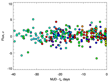
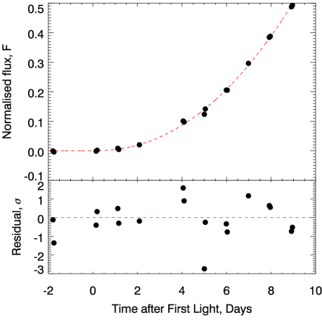
Our method is sensitive to variation in the data at very early times, i.e. very low flux levels, it is important to test for systematic effects. This was performed by averaging the points before the SN first light. Prior to the explosion, the flux level is consistent with 0, with no evidence of a systematic offset, as shown in figure 1.

An example of the data used can be found in table 3, and the entire dataset is available in online supplemental material.

Figure 3: Probability distribution contours from the fit of SN PTF09dsy. Contours enclose 99.73%, 95.45%, and 68.37% of the total probability.

Figure 4: The fit parameters for SN 2011fe as a function of the epoch range over which the fit is performed, from 2 to 18 days after first light. Top panel: The change in $n$, Middle panel: The variation in rise time, Bottom panel: The evolution of the goodness of fit statistic, $\chi^{2}$ per degree of freedom, as defined in Equation 4. The vertical dashed line shows the time at which the lightcurve reaches half of its maximum value ($t_{0.5}$)

We determine the light curve parameters for each SN Ia in our sample using the SiFTO light curve fitter (Conley et al., 2008). SiFTO manipulates the properties of a time-series SN Ia spectral energy distribution (SED) in order to best fit an observed light curve, returning the SN stretch ($s$), the time of maximum light in the rest-frame $B$-band ($t_{\mathrm{max}}$), a peak magnitude, and a colour parameter $c$ for SNe with data in more than one observed filter. We then define all phases ($\tau$) in the SN light curve as relative to this maximum-light, i.e. $\tau=t-t_{\mathrm{max}}$, thus epochs prior to maximum light have negative phases. We note that the use of SIFTO rather than (e.g.) SALT2 (Guy et al., 2007) is not critical in this paper as we do not make use of the peak magnitudes of the SNe, nor their Hubble residuals. The SiFTO stretch and SALT2 equivalent ($x_{1}$) agree very well for the same objects (e.g., Guy et al. 2010).

The spectral time-series template used by SiFTO assumes a $t^{2}$ photometric evolution in the $B$-band at phases $\tau\leq-10$ (equivalently 8-10 days post explosion for a normal SN Ia) due to a lack of accurate early SN Ia photometric data at the time the SiFTO package was written. Since in this paper we are primarily interested in the behaviour of this early time data, we remove all data with $\tau<-10$ when fitting with SiFTO. We use an iterative fitting process to do this, first using all the data to estimate the $\tau=-10$ epoch, and then refitting with data earlier than this removed.

2.3 Sample Selection

As our study requires well-sampled and relatively high signal-to-noise (S/N) data, there are several selection criteria that we make. We only allow SNe with both more than three epochs of data and more than 4 photometric points within the calculated fitting region (Section 3.3, Fig. 5), as fewer would be insufficient to constrain the free parameters in the model. Light curves with more than four days between any two consecutive points are also excluded.

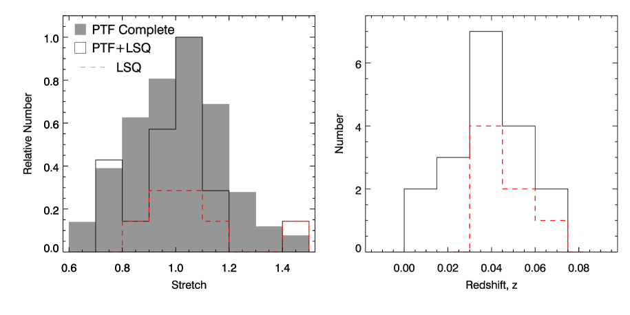
The distribution of stretch and redshift for our sample can be seen in Fig. 2. Using a Kolmogorov-Smirnov (KS) test, the stretch distribution of our sample is consistent with being drawn from the same distribution as the larger PTF sample with a probability of $91\%$. Our mean redshift, $z=0.037$, is slightly lower than that of the parent $z<0.09$ PTF sample, which has a mean redshift $z=0.056$.

3 Analysis methods

Figure 5: Schematic diagram of a SN Ia light-curve. The so called ‘dark phase’ occurs between the time of explosion, $t_{ex}$ and the time of first light, $t_{0}$. Also shown is the rise time split into its two sections: $t_{1}$ is the region within which our fitting is performed, $t_{2}$ is the time from the end of the fitting region up to maximum light

Figure 6: An example SN Ia lightcurve, best fitting model, and residual, for SN PTF11hub. The fit parameters can be found in Table 4. Uncertainties are plotted but are small, residual is shown for clarity

We now turn to the analysis methods we will use in this paper, before presenting the results in Section 4. We begin with a discussion on the parameterisation used to fit the early portion of SN Ia light curves.

3.1 Rise Time Parameterisation

The most widely used model parameterisation for the early-time SN Ia flux, $f_{model}$, as a function of time, $t$, is

$$f_{\textnormal{model}}(t)=\alpha(t-t_{0})^{n},$$ (1)

for $t>t_{0}$, and 0 otherwise. Here, $\alpha$ is a normalising coefficient, and $t_{0}$ is usually treated as the time of explosion. However, in this work we consider the possibility that the time of the first photons escaping the ejecta, and the actual explosion of the SN, are distinct, and therefore we refer to $t_{0}$ as the time of first light. Note that $t_{0}$ corresponds to the time at which the first photons leave the ejecta, which may differ from the time at which these photons can be detected by a given instrument. We do not require that the join of this model at early times to the remainder of the SN light curve be continuous.

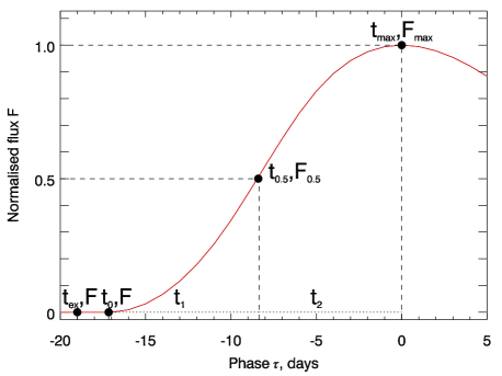
In the cases of SN 2011fe (Mazzali et al., 2014) and SN 2010jn (Hachinger et al., 2013), the precise measurement of the rise time led to some tension with spectral models, as the $t_{0}$ needed to match the observed abundances and spectral velocities is earlier than that derived from the photometry. This implies that either the models are incomplete in some way, or that there is a dark period between the time of the explosion and the emergence of the first photons from the ejecta. This is represented in Fig. 5, by the gap between $(t_{ex},F)$ and $(t_{0},F)$.

Finally, $n$ is the index of the power-law. The specific case of $n=2$ (giving a $t^{2}$ dependence) is known as the ‘expanding fireball’ model, and is used extensively in the literature as a reference model (e.g., Riess et al., 1999; Conley et al., 2006; Strovink, 2007; Hayden et al., 2010; Ganeshalingam, Li & Filippenko, 2011; González-Gaitán et al., 2012), as it provides a good empirical match to early-time SN Ia observations.

$\alpha$ is often ignored as a nuisance normalisation parameter, but physically contains information about the mass, radius, ⁵⁶Ni , and opacity of the ejecta. Pinto & Eastman (2000a) show that the (bolometric) rise time ($t_{\mathrm{rise}}$) depends on the same parameters as $\alpha$, whilst $n$ is most sensitive to the mass and distribution of ⁵⁶Ni and the shock velocity (Piro & Nakar, 2013). As $\alpha$ and $n$ depend on some of the same underlying physical parameters and processes, degeneracies between them are expected.

The simple fireball model can be justified under the assumption of constant photospheric temperature ($T$) and ejecta velocity ($v$) (Riess et al., 1999). Assuming the emitting region is hot enough and the SN is approximately represented by a black body, the standard optical passbands lie in the Rayleigh-Jeans tail of the SN SED and the SN flux will be $f\propto r^{2}T\propto v^{2}(t-t_{\mathrm{ex}})^{2}T$, which for constant $v$ and $T$ leaves $f\propto(t-t_{\mathrm{ex}})^{2}$. It should be noted that if $T$ is constant, then the bolometric luminosity rises quadratically as well. An assumption of a $t^{2}$ rise was also shown by Arnett (1982) to be reasonable, as the heating by radioactive decay should approximately balance any adiabatic losses.

These underlying assumptions are, however, unrealistic over timescales greater than a few hours. A more sophisticated treatment, following Arnett (1982), is presented in the analysis of SN 2011fe in Nugent et al. (2011), who show that the $t^{2}$ relation is expected without relying on the same assumptions. The rate of change of the internal energy can be defined as a relationship between the energy deposited by ⁵⁶Ni , the radiated luminosity and the internal radiation pressure. Their method assumes that radiation pressure dominates and that the energy from ⁵⁶Ni is thermalised throughout the ejecta. Their final, crucial assumption is that the elapsed time is much less than the ⁵⁶Ni   decay time, $t_{56}=8.8$ days. Despite the excellent fit to the data ($g_{\mathrm{P48}}$, in this case of SN 2011fe), Nugent et al. (2011) concede that this treatment is itself probably simplistic in its analysis of the diffusion wave and distribution of ⁵⁶Ni . If there is any colour evolution, then the bolometric light curve will not be well fit by the same parameters.

This is developed further by Piro (2012) who predict that the fireball model value of $n=2$ should be multiplied by a coefficient related to the ⁵⁶Ni density gradient through the ejecta and the shock velocity. This means that a single value of $n$ for all SNe Ia is not expected, and a range of $n$ is predicted instead.

Another method to probe both the structure of the ejecta and the assumptions is to investigate how the fit deviates from a $n=2$ fireball model over time. The assumptions made in deriving the fireball model (outlined in Nugent et al., 2011) are strongest soon after explosion and weaken at later times. As a result, in later sections, we consider a modified fireball model

$$f_{model}(t)=\alpha(t-t_{0})^{n_{0}+\dot{n}(t-t0)},$$ (2)

where $n_{0}$ is the rise index at time $t_{0}$ and $\dot{n}$ is a variable measuring the deviation from the fireball model as time progresses.

3.1.1 Alternative Parameterisation

A more recent parameterisation for the early light curve uses a broken power law (Zheng et al., 2013):

$$f_{model}(t)=\beta\left(\frac{t-t_{0}}{t_{b}}\right)^{\alpha 1}\left[1+\left(\frac{t-t_{0}}{t_{b}}\right)^{s(n_{1}-n_{2})}\right]^{-1/s},$$ (3)

where $\beta$ is a normalisation constant, $t_{0}$ is the time of first light, $t_{b}$ is the break time, $n_{1}$ and $n_{2}$ are the two rise indices before and after the break, and $s$ is a smoothing parameter. The motivation behind this approach is that changes in the index of a power-law are a result of drastic changes in the temperature and velocity of the fireball at very early times; the opposite of the assumptions in the fireball model. An additional contribution may come from the shock-heated cooling emission from the initial shock breakout. To date, two SNe have been fitted with this model: SN 2013dy (Zheng et al., 2013) and SN 2014J (Zheng et al., 2014; Goobar et al., 2014), in both cases predicting a faster rise time than that from a single power law model.

3.2 Fitting Methods

We perform fits of eqn (1) to our data, correcting for $1+z$ time dilation, using a grid-search minimisation of the $\chi^{2}$ statistic over our three free parameters; $\alpha$, t₀ and $n$, i.e.,

$$\chi^{2}=\sum{\left(\frac{F-f_{model}}{\sigma_{F}}\right)^{2}}$$ (4)

where $F$ and $\sigma_{\mathrm{F}}$ are the SN flux measurements and uncertainties, $f_{\mathrm{model}}$ is the model SN flux from eqn (1), and the sum runs over all the data points. We compute probabilities over a grid and report the mean value of the marginalised parameters as the best-fits, with our quoted uncertainties enclosing 68.3% of the probability. The conversion from $\chi^{2}$ to probability, $P$, is $P\propto e^{-\frac{\chi^{2}}{2}}$.

The grid size is chosen to enclose as close to 100% of the probability as is measurable. Specifically, we chose ranges of: $-15<t_{0}-t_{0}(n=2)<10$, where , $0.0<n<8.0$ and $-9<\log(\alpha)<0$. An example of the range covered, and probability distribution, can be seen in Fig. 3. We sample $\log(\alpha)$ rather than $\alpha$ to better sample low values of $\alpha$, while maintaining dynamic range.

This is a different, and slightly more direct approach to that used in Conley et al. (2006) and Ganeshalingham et al. (2011), in which Monte Carlo simulations are used to estimate the parameter uncertainties. However those analyses were performed on stacked light-curve data (rather than fitting individual objects), which requires a careful correction of the light curve shape and SN flux normalisation. This can introduce covariances between stacked data points, which demands a more sophisticated Monte Carlo like approach to handle these covariances.

The ellipticity of the contours in Fig. 3 demonstrate the covariance between the parameters in a typical fit. The strongest is found between $n$ and $\log(\alpha)$ but is present in significant strength between all of the variables.

3.3 Defining the Rise-time region

The simple rise-time model of eqn. (1) will only hold over the first few days of the SN evolution, as at some epoch the rise of the SN slows and eventually reaches a maximum point. Thus our first task is to determine over which range the model holds, and thus over which range we can fit data.

Both Conley et al. (2006) and Ganeshalingam, Li & Filippenko (2011) define the rise-time region as earlier than 10 days before $B$-band maximum light, (i.e., $\tau<-10$). This may occur at a different number of days post-explosion for different SNe Ia due to the stretching of the SN light curves. As we are not stretch-correcting the raw data in this study, prior to fitting, we instead prefer a definition relative to $t_{0}$.

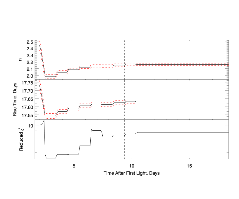
We first fit the fireball model with an initial rise time region of $\tau<-10$. This gives a first estimate of $t_{0}$ with $n=2$. We then re-fit the light curve using data ranging from 2 to 18 days after $t_{0}$, and record the values of $n$ and $t_{\mathrm{rise}}$, and the $\chi^{2}$ (Fig. 4). The discontinuous jumps in Fig. 4 are due to the inclusion of more data as the epoch range expands.

The choice of the fitting region must balance two competing constraints: there must be sufficient data to allow a meaningful rise-time fit, yet the fitting region must not reach too far into the photometric evolution where the rise-time parameterisation does not hold. Balancing these requirements across the sample, as well as taking into account the stability of the result is challenging.

In many cases, the cut-off time that best satisfied these constraints was nearly coincident with $t_{0.5}$, the time at which the SiFTO light curve was at half of its maximum value (see Fig. 5). $t_{0.5}$ is not reliant on either the stretch or a fixed number of days, so is an ideal choice as a limit of the fitting region. It is also broadly consistent with $\tau<-10$ if the light curve was stretch corrected. To ensure a consistent definition of $t_{0.5}$, after fitting, the value of $t_{0.5}$ is re-calculated using the best fit to the data. This is in most cases almost indistinguishable from that calculated from SiFTO, indicating a good match, but is free of any reliance on the later time data. Figure 6 shows the outcome of this process, a best fit to PTF 11hub.

This approach is similar to that used in González-Gaitán et al. (2012), where they define their limiting epoch as the ‘transition phase’, $\tau_{t}$, where the light curve transitions from the rise to the main body, and they find $-10\la\tau_{t}\la-8$.

Following this procedure to define our cut off, our final fit for each SN was performed on the data where $t_{0}(n=2)-2<t<t_{0.5}$ was satisfied; that is, we fit data up to two days before the time of first light, as calculated from an enforced fireball $n=2$ fit, and less than half of the maximum brightness. Imposing the lower limit was found not to affect the outcome of the fits, but removed contamination of the probability distribution from non detections.

3.4 Fits to bolometric versus filtered data

Our next task is to establish the validity of comparing fits obtained in different filters and at different redshifts, both for comparison to earlier work, and for comparison between the different surveys in our sample. Ideally we would measure the rise-time on the bolometric output of the SN, but such data are not available, and hence we need to examine any biases that might result; essentially, we are testing the effect of k-corrections. We test this by using the very well observed nearby SN Ia SN 2011fe, which has significant spectroscopic and photometric early time data.

We use 15 available pre-maximum spectra from the literature of SN 2011fe (Nugent et al., 2011; Parrent et al., 2012; Pereira et al., 2013; Mazzali et al., 2014). We measure synthetic light curves from these spectra in the $B$, $V$, $g_{\mathrm{P48}}$, $R_{\mathrm{P48}}$, and $gr_{\mathrm{LSQ}}$ filters, as well as a ‘pseudo-bolometric’ band with a wavelength range $3500-9000$Å, with each spectrum scaled so that its synthetic $g_{\mathrm{P48}}$ magnitude matched that measured from the real $g_{\mathrm{P48}}$ photometry. Using the spectral templates of Hsiao et al. (2007), this pseudo-bolometric filter contains $\simeq 70\%$ of the bolometric flux at $t_{0.5}$ (corresponding to $\tau=-8.9$), and $\simeq 72\%$ of the flux at maximum light. The wavelength range of the pseudo-bolometric filter was chosen as it is covered by most of our available spectra.

The uncertainties in our synthetic light curves come from the $g_{\mathrm{P48}}$ photometric uncertainties, with an additional systematic uncertainty added in quadrature arising from relative flux calibration errors (e..g, differential slit losses). We estimate this to be 1%. These synthetic light curves were then fit as described in Section 3.2, and the results are in Table 2.

3.4.1 The Effect of Different Filters

Figure 7: Left Panel:The flux of SN 2011fe through various filters relative to a pseudo-bolometric flux (see Section 3.4 for details) as a function of epoch. The filters are (top to bottom) $gr_{\mathrm{LSQ}}$, $g_{\mathrm{P48}}$, $B$, $V$, and $R_{\mathrm{P48}}$ filters. Right Panel: The fits to the redshifted spectra of SN2011fe, over the range of redshifts covered by our sample. The scatter around the mean redshift is consistent with the values found in the neighbouring panel. The arrows at the top of the figure show where our supernovae lie.

Table 2: Results for the SN 2011fe synthetic light curves. $\Delta n$ is the difference between n in a given filter and that of the pseudo-bolometric, i.e. $n^{filter}-n^{Pseudo-bol}$. Similarly, $\Delta t$ is the difference between t nResults in $g_{\mathrm{P48}}$  differ from Nugent et al. (2011) as a result of fitting a longer segment of the light curve.

Filter	n	$\Delta$ n	$t_{\mathrm{rise}}$,	$\Delta t_{\mathrm{rise}}$
			days	days
Pseudo-bol	$2.23$	$0.0$	$17.75$	$0.0$
$B$	$2.05$	$-0.18$	$17.13$	$-0.62$
$V$	$2.33$	$0.1$	$18.54$	$0.79$
$g_{\mathrm{P48}}$	$2.15$	$-0.08$	$17.62$	$-0.13$
$R_{\mathrm{P48}}$	$2.15$	$-0.08$	$18.14$	$0.39$
$gr_{\mathrm{LSQ}}$	$2.20$	$-0.03$	$17.94$	$0.19$

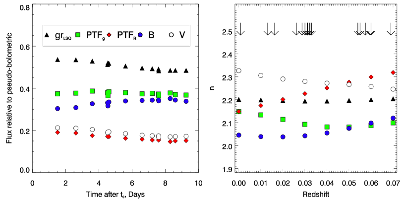
The results show some differences between different filters, due to rapid evolution in the spectral features in each band. Fig. 7 shows how the flux in each filter, relative to pseudo-bolometric flux at that epoch, changes with time. The $g_{\mathrm{P48}}$ band shows an almost constant flux ratio, but $R_{\mathrm{P48}}$ decreases with time, while the $B$-band increases. The pseudo-bolometric value, $2.23$ is greater than that in $g_{\mathrm{P48}}$, and greater than 2, in agreement with the findings of Piro & Nakar (2014). The broadest filter, $gr_{\mathrm{LSQ}}$, is obviously the closest to bolometric, but also shows a decreasing flux ratio. Note that earlier work has predominantly used data either in, or corrected to, the $B$-band. Table 2 shows that this fit has an $n$ closest to 2; however, it is significantly lower than the values in the other filters, and is not consistent with the pseudo-bolometric value.

In an attempt to further understand the colour evolution and its effect on $n$, templates from SALT2 (Guy et al., 2007) and Hsiao et al. (2007)/SiFTO(Conley et al., 2008) were analysed, however, the nature of the investigation probes the very earliest epochs, where there have been few spectral observations. For example, the earliest Hsiao et al. (2007) templates pre-maximum are based on 6 spectra with an average epoch of $\tau=-11.6$ days. Because of this, and despite being a single example, the data from SN 2011fe are the best resource available at very early times. Comparing with SN 2013dy (Zheng et al., 2013), the colour evolution is similar, although SN 2011fe exhibits a stronger Ca II IR triplet compared with SN 2013dy within the first 2 days. This does not fall within any of our filters, but falls within the pseudo-bolometric range.

In summary, by considering the different fits to our simulated photometry, we estimate the systematic effect of using different filters to be $n\pm 0.1$

3.4.2 The Effect of Redshift

As our sample lies across a range of redshifts, we also need to ascertain the impact that this has on the colour evolution. To do this, we performed the same procedure as in section 3.4.1, redshifting the spectra each time, up to our maximum redshift of $z=0.07$ before fitting. The results of these tests can be seen in the right-hand panel of figure 7.

We find that the broad $gr_{\mathrm{LSQ}}$ filter provides data that is very stable with redshift, the value of $n$ remaining almost static. Leaving the rest-frame, the measured $n$ in $R_{\mathrm{P48}}$ and $g_{\mathrm{P48}}$ diverges, with the $R_{\mathrm{P48}}$ increasing and the $g_{\mathrm{P48}}$ decreasing more steadily. The scatter around the mean redshift ($z=0.036$) is consistent with the dispersion between filters in table 2.

In summary, we estimate the systematic effect of redshift to be reflective of that from using different filters, since the low redshifts do not shift the spectra by more than the width of our filters, that is, a systematic effect of at most $n\pm 0.1$

3.4.3 The Effect of Extinction

We also performed these checks after reddening the spectra by $E(B-V)=1$ and found no significant deviation in results. Additionally, inspecting the spectra at maximum light of each PTF object in our sample, we find evidence of Na I D absorption in only two SNe (PTF11gdh and PTF12gdq). These are discussed in Section 4 but do not appear to be unusual events.

Figure 8: Left Panel: Histogram showing the distribution of rise times for our sample leaving $n$ as a free parameter. The solid grey histogram shows the raw rise-time, while the unshaded histogram shows the rise-time corrected for stretch. Right Panel: The histogram of the best-fit rise-index ($n$) values. The distribution has $n_{mean}=2.36\pm 0.13$ and $n_{median}=2.31$ with a slight positive skew.

4 Results

We now present the results of applying our fitting methods (Section 3.2) to our data sample (Section 2.3). We first discuss the rise-time analysis, followed by the rise index. Our results can be found in Table 4.

4.1 The SN Ia rise time

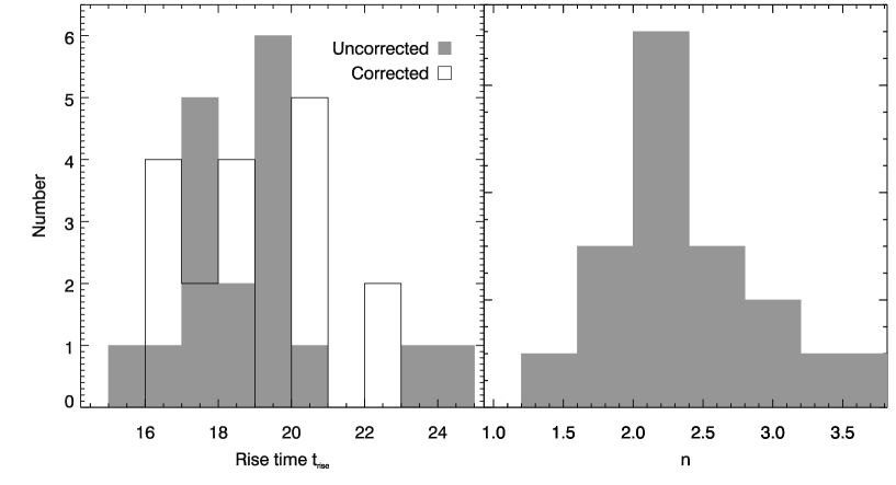
The average rise-time of the 18 SNe Ia in our sample with $n$ a free parameter in the fit, is $t_{\mathrm{rise}}=18.98\pm 0.54$ days, or $t_{\mathrm{rise}}=18.97\pm 0.44$ days if the rise-times are stretch-corrected, where the uncertainties in both cases are the standard error on the mean (We exclude one SN, PTF12emp, from this latter calculation as there is insufficient data to reliably estimate a stretch.) For the stretch correction, we use SIFTO to measure the stretch based on photometry later than $\tau=-10$, and so it is independent of the shape of the early light curve. These values are longer than those found in previous work. Assuming $n=2$, the mean rise-times are $t_{\mathrm{rise}}=17.86\pm 0.42$ days uncorrected and $t_{\mathrm{rise}}=17.90\pm 0.33$ days, after stretch correction. The $n=2$ rise times are shorter in both cases. These values are consistent with Ganeshalingam, Li & Filippenko (2011), but lower than Conley et al. (2006) and higher than those found in both Hayden et al. (2010) and González-Gaitán et al. (2012) by $3\sigma$.

Figure 9: The difference between the measured $t_{\mathrm{rise}}$ and the $t_{\mathrm{rise}}$ expected from our SN template based on the fit stretch, plotted against the stretch. The coloured points denotes a binning by the rise index. Red circles are $n>2.4$, green triangles $1.9<n<2.4$, and blue squares $n<1.9$. Higher stretch SNe Ia have a $t_{\mathrm{rise}}$ that is faster than that implied by the stretch-corrected template $t_{\mathrm{rise}}$.

Figure 10: Stretch vs rise time. The black points are those fitted with a free $n$ parameter, the hollow points are those where the fitting has been constrained to $n=2$.

Figure 11: Top Panel:  $n$ vs $t_{1}$, in the region fitted, $n$ correlates with the length of time from $t_{0}$ to $t_{0.5}$. Bottom Panel: $t_{2}$ vs $t_{1}$, no strong correlation can be seen between the early $t_{1}$ and late $t_{2}$ parts of the light curve.

The histogram of the rise-time distributions can be found in Fig. 8. Strovink (2007) previously suggested that there may be two rise time modes, once the rise times have been corrected for the overall shape of the light curve (using the fall time). We do not find any evidence for this using either $n=2$ or $n$-free.

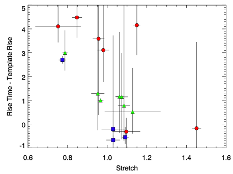
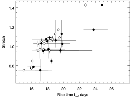
Hayden et al. (2010) and Ganeshalingam, Li & Filippenko (2011) both find that the fraction of their sample that are slowest to decline after peak are amongst the fastest to rise. Both studies therefore parameterise the width of the light curve using two stretch parameters, one pre- and one post-maximum. Ganeshalingam, Li & Filippenko (2011) also find that the luminous SNe Ia have a faster rise than expected based on a single stretch value. We see a similar trend in Fig. 9, also lower stretch SNe appear to have slower light curves than would be expected from a single stretch.

Figure 12: Left Panel:  Stretch vs $t_{1}$, no strong correlation can be seen. Right Panel:  Stretch vs $t_{2}$, a clear correlation is visible. This is expected as the stretch was measured using data within this region, the strength of the correlation is slightly weaker than expected.

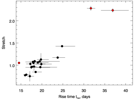
In Fig. 10, we show the relation between stretch (again calculated without the very early photometric data) and $t_{\mathrm{rise}}$. A correlation is expected and observed in the data. The results are also shown for when $n=2$ showing, on average, shorter rise times.

The rise-time can be decoupled into two components: $t_{1}$, the time between first light ($t_{0}$) and the time of half maximum ($t_{0.5}$), and $t_{2}$, the time between $t_{0.5}$ and $t_{\mathrm{max}}$  (shown in Fig. 5). As can be seen in Fig. 11, surprisingly, these two timescales do not show a particularly strong dependence, having a Pearsons Correlation Coefficient $P=0.61$, and when imposing a stretch cut commonly used in cosmology, $0.7\leq s\leq 1.3$ (Conley et al., 2011), which excludes LSQ12gpw, this drops to $0.43$. As the SiFTO fit includes data from $\tau>10$, which is roughly consistent with $t_{0.5}$, it is unsurprising that there is a strong correlation between $t_{2}$ and stretch (Fig. 12), with $P=0.89$. However, there is also no strong relationship between stretch and $t_{1}$ (Fig. 12) ($P=0.57$, which weakens to $P=0.34$ when imposing a stretch cut).

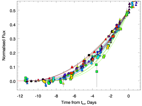
The diversity of the early time light curves in our sample can be seen in Fig. 13. The light curves have been stretch corrected and normalised, and shifted to have a coincident $t_{0.5}$. Whilst when stretch corrected, in the $t_{2}$ distribution the scatter is reduced, the data in $t_{1}$ still show a large amount of variation (Fig. 13). This variation, even after stretch correction, may have been lost within instrumental noise in previous surveys. To avoid introducing additional systematics due to misinterpreting this scatter, care must be taken when using SNe Ia data in this region for cosmology as the variation is significant.

4.2 The Rise Index - ‘$n$’

Figure 13: Our sample of 17 SNe Ia (PTF12emp excluded, see Sec. 4.1), normalised, stretch corrected and shifted to have coincident $t_{0.5}$. Note the diversity in the early SNe Ia light curves even after stretch correction

Figure 14: The best-fit ‘$n$’ and uncertainty for each SN in the sample. Hollow squares are $gr_{\mathrm{LSQ}}$observations, solid circles are $R_{\mathrm{P48}}$and hollow circles are $g_{\mathrm{P48}}$. The dotted lines indicate $n=2$ and the mean of the sample, $n_{mean}=2.44\pm 0.13$. The crosses show the location of the points corrected to the ‘bolometric’ value of $n$, if the SN 2011fe correction (Table 2) holds for other SNe

Figure 15: The fitted n plotted against the time of the first observation, relative to $t_{0}$ corrected for redshift. LSQ SNe are shown in red (filled) and PTF are shown in white (hollow). The best fit to the data is overplotted.

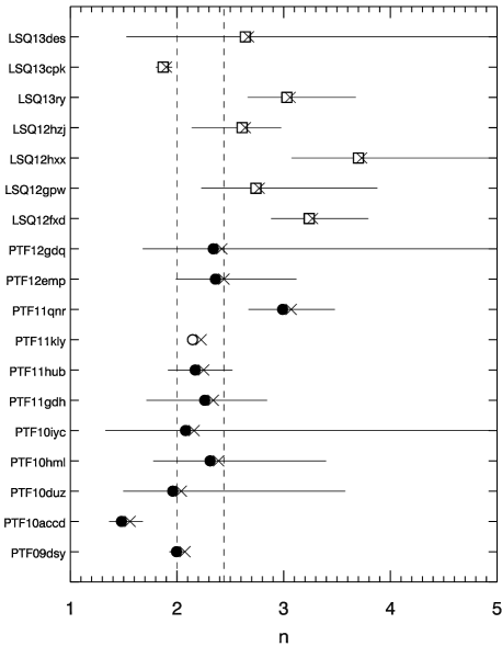
The distribution of the $n$ parameter, which can be seen in Fig. 8, has a mean of $n=2.44\pm 0.13$ and a tail in the distribution towards higher $n$. When corrected to a pseudo-bolometric value, as discussed in Section 3.4, this becomes $n=2.50\pm 0.13$. Both mean values, corrected and uncorrected, are not consistent with the $n=2$ fireball model, although individual SNe Ia within the sample are consistent with $n=2$ (Table 4); the $n$ values broken by SN name are shown in Fig. 14. To compare with previous work (Table LABEL:RT_table), our $n$ value is marginally consistent with Ganeshalingam, Li & Filippenko (2011), who use the low-redshift LOSS sample and find $n=2.2^{+0.27}_{-0.19}$. Our result is inconsistent with more recent higher redshift studies, Hayden et al. (2010) or González-Gaitán et al. (2012). Furthermore, the recent study of SN 2014J has yielded a rise index of $n=2.94\pm 0.20$ (Zheng et al., 2014). This lends further evidence that there is not only a range of $n$, but that the centre of the distribution is located at values $n>2$. This result supports the finding of Piro & Nakar (2014) that a $t^{2}$ rise is not a generic property of SNe Ia.

As mentioned in Section 3.4.3, we see non-zero Na I D absorption lines at the position of the host galaxy in the low-resolution spectra in in two SNe; PTF11gdh and PTF12gdq. However, we cannot tell whether this is from the host or from CSM interaction but the measurements of $n$ and $t_{\mathrm{rise}}$ are not different from the bulk of the sample. We do not find these SNe to occupy any unusual position in any of the parameter space we investigate. Both have a value of n that is consistent with the mean value within the calculated uncertainties.

We find no evidence of a correlation between $n$ and stretch (Fig 16, left panel). González-Gaitán et al. (2012) found a weak trend, with larger stretches corresponding with higher $n$. While both $t_{\mathrm{rise}}$and Stretch do not correlate strongly with $n$, as can be seen in Fig 16, there is a clear correlation between $t_{1}$ and $n$ (Figure 11, top panel), with the lowest rise indices corresponding to the shortest initial time spans.

A distribution of $n$ values centred above $2$ agrees well with previous work on individually fitted SNe (Nugent et al., 2011; Hachinger et al., 2013; Zheng et al., 2013, 2014). However, these fits were done on rise time regions of varying sizes, it is for this reason that our value of $n$ for SN 2011fe differs from that of Nugent et al. (2011); in Fig. 4, when the data range fitted is the same, the values are fully consistent. Thus direct comparisons between studies are difficult, as a shorter, earlier fitting region probes a shallower ejecta region, raising the prospect of a time dependent index.

4.2.1 A Time Dependent Index - $`\dot{n}$’

Figure 4 shows that the $n$ measured changes over time, as more data is added the behaviour of $n$ in Fig. (4), is evidence that this is occurring. This effect explains the difference in $n$ measured in this work ($n=2.15\pm 0.02$, for $t_{0}\leq t\leq t_{0.5}$) and Nugent et al. (2011) ($2.01\pm 0.01$ for $t_{0}\leq t\leq t_{0}+3$) procedure as outlined in Section 3.2, substituting eqn. 2 for eqn. 1.

We find evidence for a positive $\dot{n}$ in most SNe in our sample, with a mean value of $\dot{n}=0.011\pm 0.004\,d^{-1}$ (where the uncertainty is the standard error on the mean) and a weighted mean value of $\dot{n}=0.011\pm 0.001\,d^{-1}$. Specifically, in the case of SN 2011fe with n as a free parameter we find $n_{0}=2.02\pm 0.02$, consistent with Nugent et al. (2011), and an $\dot{n}=0.011\pm 0.001\,d^{-1}$. This positive $\dot{n}$ (in both cases) reflects that fitting equation 1 we find the mean $n$ greater than 2. We find some evidence that the SNe that have observations longest after explosion are those which, in general, have the largest $\dot{n}$; that is, the largest rate of deviation away from the fireball model. This may be driven physically by the later time data being driven by deeper ejecta layers.

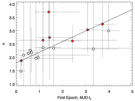
This time dependence of $n$ can also be seen in Fig 15. When the first observation of a SN is made earlier, the $n$ is lower, due to the different ejecta conditions. Applying a linear fit, an intercept of $n=1.8\pm 0.2$ is found, and a slope of $m=0.39\pm 0.15$, making the trend significant to $2.6\sigma$. When the observations begin at a later epoch, there is a smaller contribution from the ⁵⁶Ni in the upper most layers, changing the measured $n$.

Figure 16: Left Panel: $n$ vs Stretch for our sample, no evidence of a correlation is found. Right Panel: $n$ and $t_{\mathrm{rise}}$do show some evidence of a relationship, but with low significance.

4.2.2 Broken Powerlaw

We also performed a fit to SN 2011fe using equation 3. Unlike Zheng et al. (2013) and Zheng et al. (2014) we find no evidence for a break in the light curve. The data from SN 2011fe contains 6 data points within the first three days after the explosion (i.e. before a ‘break time’; $t_{b}^{2013dy}=3.14\pm 0.30\,d$ and $t_{b}^{2014J}=2.61\pm 0.20\,d$), however these are clustered in three epochs, and it may be that sub-day cadence is needed in this early time to be sensitive to broken power laws.

5 Discussion

In Piro (2012), the first four days of data from SN 2011fe were analysed and the implications of a power-law dependence explored, considering the dynamics and thermodynamics of the expanding ejecta in shells. At early times, the emitted luminosity originates from a shell between $\simeq 0.01$ and $0.3M_{\odot}$. Piro (2012) calculate that the power-law scaling for the bolometric luminosity goes as $L(t)\propto t^{2(1+1/\gamma+\chi)/(1+1/\gamma+\beta)}$ for $t\la t_{56}$, with the polytropic index, $\gamma=3/2$ for non-relativistic electrons ($\gamma=3$ for relativistic electrons), and for a radiation pressure dominated shock, $\beta=0.19$ which controls the rate of change of the shock velocity, while $\chi$ characterises the ⁵⁶Ni distribution in the ejecta shell. To change the $n$ value, either $\chi$ or $\beta$ must change. Simplifying the expression by setting $\chi=0$ results in $n\simeq 1.8$. This value is consistent with Conley et al. (2006), despite the fitting region being twice the size of the $4$ days for SN 2011fe. If we treat the region from $t_{0}$ to $t_{0.5}$ as one shell, as in this parameterisation, increasing $n$ is possible by increasing $\chi$, and having deeper ⁵⁶Ni dominating the rise. However smaller $n$ are more problematic to explain.

It should be noted that, in Fig 15, the intercept of the best fit, at $n=1.8$, is consistant with the above case from Piro (2012). This value is in tension with the findings of higher $n$ values in SN 2013dy and SN 2014J and the justification that the value of $n$ found was due to the unprecedented early discovery and followup. Clearly, data on further SNe collected very soon after first light are needed.

Only one of the SNe in our sample has $n<1.8$, PTF10accd, and the small uncertainties make it inconsistent with both $n=2$ and the lower limit of Piro (2012) ($n=1.8$). It should be reiterated that the bolometric value is expected to be larger than the values in $R_{\mathrm{P48}}$ or $g_{\mathrm{P48}}$; however, from our tests in Section 3.4 this would not make PTF10accd consistent with $n=1.8$.

This result has two possible implications depending on $\chi$. If $\chi<0$, either ⁵⁶Ni dominates the makeup of the outer ejecta, or the flux originates from elsewhere; potentially from some CSM interaction. Alternatively, the optical luminosity of the shock-heated cooling light curve may be dominant as this is expected to have $n=1.5$. If $\chi\geq 0$, then the shock is not radiation pressure dominated and $\beta$ may vary, or the delayed detonation transition (DDT) model, from which the velocity gradient is calculated (Piro, Chang & Weinberg, 2010) is an incomplete description of this process. Other models, such as He double-detonation (Fink et al., 2010) or the collision model (Kushnir et al., 2013; Dong et al., 2014) present different treatments of the velocity gradient.

More recent work (Piro & Nakar, 2013) investigates the contribution of ⁵⁶Ni heating, both directly and from the diffusive tail, throughout the ejecta. In the appendices of Piro & Nakar (2013), rather than treating shells of material individually, integrals are evaluated over the entire ejecta. This leads to an altogether more complex picture of the energy generation, which depends on the relative fraction of ⁵⁶Ni throughout the ejecta, as given by

$$X_{56}(x)=\frac{1}{1+\exp[-\beta(x-x_{1/2})]},$$ (5)

Figure 17: Contours showing the fitted $n$ parameter of a bolometric light curve generated by using different values of $\beta$ and $x_{1/2}$ in Equation 5. A large range of $n$ values are recovered, but extreme values of $\beta$ and $x_{1/2}$ may not be physical.

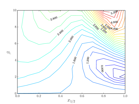
where $x$ is a measure of depth within the ejecta, $x_{1/2}$ is the point at which the ⁵⁶Ni fraction is half at that of its value at peak, and $\beta$ is the steepness of the rise in the distribution. Generating a bolometric luminosity using this parameterisation, it is possible to attain a large range of $n$ values, when fitting a power-law (Fig. 17). The physical limits of this parameter space are uncertain, and fitting a number of SNe directly with this has yielded values in the ranges $6\leq\beta\leq 8$ and $x_{1/2}\simeq 0.9$. The mean value of our study indicates that on average the envelope is less well mixed and there is an abrupt change within the ⁵⁶Ni distribution in most cases in the sample.

However, at very early times, fitting with a simple power law, the fit is poor, as the light curve is better described as an exponential (Piro & Nakar, 2014). The timescales for this discrepancy are short, and beyond the reach of this work. However, this may be the apparent ‘break’ in the power law seen in 2013dy and 2014J (Zheng et al., 2013, 2014) - an exponential rise turning into a power law at later times. Our finding that $\dot{n}$ is, in general, positive, supports this.

In Fig. 4 as the cutoff drops below $\sim 3.5$ days, $n$ is consistent with 2, in agreement with Nugent et al. (2011). This value differs from our final result for SN 2011fe because the shorter time period used only probes a shallow region of the ejecta. At very early times, the rise index jumps to higher values. This difference could be hinting towards a broken power-law as outlined in Section 2.1, Equation 3, or something that resembles one (Piro & Nakar, 2014); however, attempting to fit this model to SN 2011fe is unsuccessful; as there is not enough data at very early times to constrain the 7 free parameters.

At present, none of these various models make any predictions that would explain the decoupling of the early and late part of the rise seen in our data. However, a scatter in the measured photometric rise time can be explained by invoking a ‘dark phase’, between explosion and first light (Fig 5), due to deep ⁵⁶Ni deposits. More work is needed to further understand this phenomena, using the methods previously applied to SN 2011fe and SN 2010jn (Mazzali et al., 2014; Hachinger et al., 2013), on future samples of well observed SNe. The dark time for SN 2010jn was estimated to be  1.4 days, and that of SN 2011fe to be  1 day. As we expect that, for a given value of $x_{1/2}$, higher $n$ values are consistent with a steeper gradient, $\beta$, higher $n$ values should be consistent with a longer dark time. This effect is seen in these two SNe; SN 2011fe has an $n=2.15\pm 0.02$ (our value is used over that of Nugent et al. (2011) as the fitted regions are more comparable) and SN 2010jn $n=2.3\pm 0.6$.

As the available light curves can be well fit by using a simple power law, more high quality photometric and spectroscopic data is needed to distinguish between the models, and to see expected deviations from power laws (Zheng et al., 2013; Goobar et al., 2014). Ideally, future work would be able to concentrate on bolometric data, which is now becoming possible (Scalzo et al., 2014).

Tanaka et al. (2008) find a significant range of ⁵⁶Ni abundances in the outer ejecta of a sample of SNe Ia, which is taken as one of the causes of early time spectral variation in SNe Ia; they also suggest this could have photometric consequences. Our work clearly demonstrates that there is indeed a photometric shape variation, and that a cause of this is in ⁵⁶Ni deposition between SNe Ia, as suspected.

5.1 Type Ia ‘CSM’ Supernovae

As considered in the previous subsection, one of the possible reasons for a SN to have an ‘anomalous’ rise would be an energy contribution from interaction with CSM material (Falk & Arnett, 1977). Silverman et al. (2013) noted that the rise of SNe Ia-CSM tends to be significantly longer than a typical SNe Ia, following a simple photon diffusion argument - not only does a photon have to diffuse through the ejecta, but also significant amounts of CSM as well. In that respect, Ofek et al. (2014a) showed that in SNe Type IIn there is a possible correlation between rise time and peak luminosity.

We therefore examined PTF SNe Ia-CSM from the sample of Silverman et al. (2013) (7 SNe). Only 3 have sufficiently good photometry to provide acceptable fits, even after introducing constraints on the fitting. These fits assumed the fireball model, ($n=2$), and the results of measuring the rise time can be seen in Figure 18. One of these SNe, PTF12efc is a ‘typical’ broad and bright SNe-CSM, although having an extreme rise time and stretch, and seems to lie in agreement with the best fit to the distribution of normal SNe Ia. PTF10iuf also has a long rise and large stretch but a higher stretch than would be predicted from the measured rise time. Despite lying on or near the correlation of ‘normal’ SNe Ia, there seems to be no reason for this to be the case - the rise is shaped by different physical processes over different timescales.

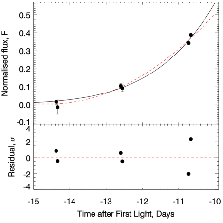
PTF11kx has a rise time of only $t_{r}^{n=2}=14.5\pm 0.2$ (Fig. 19), but a measured stretch of $s=1.05$. In Dilday et al. (2012), a rise time of $\sim 20$ days is assumed; note that a shorter rise time means that the ejecta will be smaller at a given epoch. Consequently, the ejecta mass calculated using the previous estimate ($\sim 5.3\textnormal{M}_{\odot}$.) is too large, and should be $\sim 80\%$ of that value, $\sim 4.3\textnormal{M}_{\odot}$, making the same assumptions as in the supplemental information of Dilday et al. (2012). As well as performing a fit holding $n=2$ a grid-search was done to find the best fit where $t_{r}=20$ days (Fig. 19). With a fixed rise, the best fit index was $n=6.2\pm 0.5$, this result is not physical for a ‘normal’ SN Ia, but SNe Ia-CSM have an additional contribution to their light from the collision of their ejecta with the CSM; this converts the kinetic energy in the ejecta into hard X-ray photons, which in the presence of sufficient optical depth can be converted into optical light (e.g. Chevalier & Irwin, 2012; Svirski, Nakar & Sari, 2012; Ofek et al., 2014a). With this in mind, it may be expected for SNe Ia-CSM to have abnormal rise properties. Until a confirmed SN Ia-CSM is observed with enough precision to enable a relaxing of $n$, few constraints can be placed on the effect of CSM on a rising light curve.

Figure 18: Stretch vs Rise time with 3 SNe Ia identified as CSM by Silverman et al. (2013) plotted in red

Figure 19: PTF11kx lightcurve and two fits to the data. A fit with fixed $n=2$ is shown in red (dashed), and a fit with a fixed rise of $t_{\mathrm{rise}}=20.0$ days is shown in black.

6 Conclusions

In this work we have used 18 type Ia supernovae (SNe Ia) from the Palomar Transient Factory (PTF) and the La Silla-QUEST variability surve (LSQ) to measure the rise time ($t_{\mathrm{rise}}$) (the time between first light $t_{0}$, and maximum light $t_{max}$) and rise index ($n$), where $f=(t-t_{0})^{n}$. Our main conclusions are:

1. The rise index, $n$, of our sample shows significant variation ($1.48\leq n\leq 3.70$), with the mean of the distribution $n=2.44\pm 0.13$, and $n=2.5\pm 0.13$ when correcting to a pseudo-bolometric value (Section 4.2), both inconsistent with a simple fireball model ($n=2$) at a $3\sigma$ level. This implies that current understanding of the ⁵⁶Ni distribution or shock velocity through the ejecta is incomplete, and that more complex physically motivated parameterisations may be needed in future.

2. We find that when the rise index is allowed to vary with time from $n=2$, $\dot{n}$ is in general positive, with an average value of $\dot{n}=0.011\pm 0.004\,$ day^-1. Supporting a time dependant $n$, is the finding that SN discovered later after first light have, in general a larger value of $n$, whereas those discovered soonest after $t_{0}$ have lower values.

3. The average $t_{\mathrm{rise}}$ of our sample is $t_{\mathrm{rise}}=18.98\pm 0.54$ days, and $t_{\mathrm{rise}}=18.97\pm 0.43$ days, when correcting for light curve width. We find no evidence for two rise time modes in our sample. These are longer than would ordinarily be found by enforcing $n=2$.

4. The broadest light curves have a $t_{\mathrm{rise}}$ that is faster than that of our stretch-corrected light curve template, which enforces $n=2$ in its construction. In agreement with previous studies, we find that a ‘two stretch’ model fits the data better. In contrast to current two-stretch fitting methods, which separate the light curve into the pre- and post-maximum sections ($t<t_{max}$ and $t>t_{max}$ respectively), the most significant variation occurs at the very earliest epochs ($t<t_{0.5}$, where $t_{0.5}$ is the time at which the SNe reaches half of its maximum, or phases $\tau<-10$ d).

5. We therefore decouple the rise time into two components: $t_{1}$ (where $t_{1}=t_{0.5}-t_{0}$) and $t_{2}$ (where $t_{2}=t_{max}-t_{0.5}$). These time-scales are not correlated with each other (Fig. 11); furthermore $t_{2}$ is strongly correlated with stretch, whereas $t_{1}$ is not. As a result, stretch correcting using a single stretch is ineffective in reducing the dispersion in the earliest portion of the light curve (Fig. 13).

6. These two regions are separated by the approximate location of the point at which energy deposition and radiation are equal, meaning that the physical conditions are distinct.

7. Using models from Piro & Nakar (2013), we show that potential variation in the shape of the ⁵⁶Ni  distribution within the SN ejecta can explain the measured range of $n$ and $t_{\mathrm{rise}}$.

8. SNe Ia showing evidence of strong interaction with circumstellar material (CSM) have long rise times. However a notable member of this subclass, PTF11kx, has an extremely short rise, $t_{\mathrm{rise}}=14.5\pm 0.5$ days, when fitted with a fireball model ($n=2$).

Further work should concentrate on further understanding the variation, and on which other observable quantities it depends. For this, a large sample of SNe Ia with high quality photometric and spectroscopic data must be assembled. The presence of high velocity features, Si II velocities and colour evolution may hold valuable information, particularly if the variation at very early times is misunderstood when used for cosmology.

7 Acknowledgements

We wish to thank the Reviewer for a careful and considered reading, and thorough and helpful report.

MS acknowledges support from the Royal Society and EU/FP7-ERC grant no [615929].

KM is supported by a Marie Curie Intra European Fellowship, within the 7th European Community Framework Programme (FP7).

This research used resources of the National Energy Research Scientific Computing Center, which is supported by the Office of Science of the U.S. Department of Energy under Contract No. DE-AC02-05CH11231.

E.O.O. is incumbent of the Arye Dissentshik career development chair and is grateful to support by grants from the Willner Family Leadership Institute Ilan Gluzman (Secaucus NJ), Israeli Ministry of Science, Israel Science Foundation, Minerva, Weizmann-UK and the I-CORE Program of the Planning and Budgeting Committee and The Israel Science Foundation.

Observations obtained with the Samuel Oschin Telescope at the Palomar Observatory as part of the Palomar Transient Factory project, a scientific collaboration between the California Institute of Technology, Columbia University, Las Cumbres Observatory, the Lawrence Berkeley National Laboratory, the National Energy Research Scientific Computing Center, the University of Oxford, and the Weizmann Institute of Science.

Some of the data presented herein were obtained at the W.M. Keck Observatory, which is operated as a scientific partnership among the California Institute of Technology, the University of California and the National Aeronautics and Space Administration. The Observatory was made possible by the generous financial support of the W.M. Keck Foundation.

This research was made possible through the use of the AAVSO Photometric All-Sky Survey (APASS), funded by the Robert Martin Ayers Sciences Fund.

Table 3: Table of example data for one SN, PTF09dsy. Data for the full sample can be found in online supplemental material

SN	MJD	Counts	$\Delta$ Counts	Filter	Zero Point	Redshift
PTF09dsy
	55054.441	-67.7	98.2	$R_{\mathrm{P48}}$	27.000	$0.0131\pm 0.001$
	55054.460	-68.7	72.3	$R_{\mathrm{P48}}$	27.000	$0.0131\pm 0.001$
	55055.460	480.0	101.0	$R_{\mathrm{P48}}$	27.000	$0.0131\pm 0.001$
	55055.472	457.2	67.6	$R_{\mathrm{P48}}$	27.000	$0.0131\pm 0.001$
	55059.443	8599.9	93.5	$R_{\mathrm{P48}}$	27.000	$0.0131\pm 0.001$
	55059.463	8603.4	94.4	$R_{\mathrm{P48}}$	27.000	$0.0131\pm 0.001$
	55061.434	16360.3	142.9	$R_{\mathrm{P48}}$	27.000	$0.0131\pm 0.001$
	55061.459	16634.9	104.1	$R_{\mathrm{P48}}$	27.000	$0.0131\pm 0.001$
	55063.438	27290.6	123.8	$R_{\mathrm{P48}}$	27.000	$0.0131\pm 0.001$
	55063.483	26937.5	143.1	$R_{\mathrm{P48}}$	27.000	$0.0131\pm 0.001$
	55066.421	38663.8	301.7	$R_{\mathrm{P48}}$	27.000	$0.0131\pm 0.001$
	55066.466	39415.6	192.0	$R_{\mathrm{P48}}$	27.000	$0.0131\pm 0.001$
	55069.410	46253.4	201.1	$R_{\mathrm{P48}}$	27.000	$0.0131\pm 0.001$
	55069.455	46201.3	209.2	$R_{\mathrm{P48}}$	27.000	$0.0131\pm 0.001$
	55080.373	30495.7	222.8	$R_{\mathrm{P48}}$	27.000	$0.0131\pm 0.001$
	55080.461	29730.6	248.6	$R_{\mathrm{P48}}$	27.000	$0.0131\pm 0.001$
	55087.350	24598.7	169.6	$R_{\mathrm{P48}}$	27.000	$0.0131\pm 0.001$
	55087.395	24978.9	178.0	$R_{\mathrm{P48}}$	27.000	$0.0131\pm 0.001$
	55089.381	23637.7	162.0	$R_{\mathrm{P48}}$	27.000	$0.0131\pm 0.001$
	55089.425	23756.2	197.7	$R_{\mathrm{P48}}$	27.000	$0.0131\pm 0.001$
	55093.351	20758.2	147.4	$R_{\mathrm{P48}}$	27.000	$0.0131\pm 0.001$
	55093.395	20267.0	159.0	$R_{\mathrm{P48}}$	27.000	$0.0131\pm 0.001$
	55095.338	18196.5	117.7	$R_{\mathrm{P48}}$	27.000	$0.0131\pm 0.001$
	55095.382	18400.1	168.8	$R_{\mathrm{P48}}$	27.000	$0.0131\pm 0.001$
	55107.311	8207.5	146.7	$R_{\mathrm{P48}}$	27.000	$0.0131\pm 0.001$
	55107.355	8001.8	136.7	$R_{\mathrm{P48}}$	27.000	$0.0131\pm 0.001$

Table 4: Table of Results

SN	$t_{max},$	$t_{\mathrm{rise}}$,	$n$	$\dot{n}$	Stretch	$\chi^{2}_{\textnormal{DOF}}$	R.A	Dec.	Filter
	MJD	days					(J2000)	(J2000)
PTF09dsy	$55070.4\pm 0.1$	$15.98\pm 0.20$	$2.00^{+0.08}_{-0.07}$	$0.0^{+0.13}_{-0.01}$	$0.80\pm 0.01$	0.58	3:33:22.1	-04:59:55.2	PTF48R
PTF10accd	$55556.0\pm 0.2$	$18.17^{+0.46}_{-0.32}$	$1.48^{+0.19}_{-0.12}$	$-0.02\pm 0.01$	$1.11\pm 0.02$	0.78	02:13:30.4	46:41:37.2	PTF48R
PTF10duz	$55285.0\pm 0.2$	$17.5^{+3.7}_{-1.0}$	$1.96^{+1.5}_{-0.46}$	$-0.005^{+0.02}_{+0.01}$	$1.00\pm 0.03$	1.88	12:51:39.5	14:26:18.7	PTF48R
PTF10hml	$55352.3\pm 0.1$	$19.4^{+2.7}_{-1.5}$	$2.31^{+1.08}_{-0.53}$	$0.01^{+0.01}_{-0.02}$	$1.07\pm 0.02$	1.50	13:19:49.7	41:59:1.6	PTF48R
PTF10iyc	$55361.5\pm 0.1$	$19.4^{+4.4}_{-1.4}$	$2.08^{+2.00}_{-0.70}$	$0.00^{+0.02}_{-0.03}$	$1.10\pm 0.02$	1.04	17:09:21.8	44:23:35.9	PTF48R
PTF11gdh	$55744.1\pm 0.1$	$19.57\pm 1.8$	$2.26^{+0.58}_{-0.55}$	$-0.005\pm 0.01$	$1.07\pm 0.03$	1.25	13:00:38.1	28:03:24.1	PTF48R
PTF11hub	$55770.0\pm 0.2$	$16.50^{+0.96}_{-0.76}$	$2.17^{+0.35}_{-0.26}$	$0.005\pm 0.01$	$0.80\pm 0.01$	1.17	13:12:59.5	47:27:40.3	PTF48R
PTF11kly/SN2011fe	$55814.3\pm 0.1$	$17.59\pm 0.1$	$2.15\pm 0.02$	$0.011\pm 0.001$	$0.965\pm 0.009$	$8.06$	14:30:5.8	54:16:25.2	PTF48g
PTF11qnr	$55902.3\pm 0.1$	$17.01^{+1.0}_{-0.7}$	$2.99^{+0.49}_{-0.32}$	$0.025^{+0.01}_{-0.005}$	$0.79\pm 0.04$	1.57	22:44:25.4	-00:10:2.0	PTF48R
PTF12emp	$56080.9\pm 0.4$	$19.9^{+1.9}_{-1.0}$	$2.36^{+0.76}_{-0.37}$	$0.01^{+0.01}_{-0.01}$	$1.13\pm 0.14$	3.52	13:13:53.7	34:06:59.7	PTF48R
LSQ12fxd	$56246.4\pm 0.1$	$23.8^{+1.8}_{-1.3}$	$3.24^{+0.53}_{-0.36}$	$0.02^{+0.02}_{-0.2}$	$1.17\pm 0.01$	2.77	05:22:17.0	-25:35:47.0	LSQgr
PTF12gdq	$56116.3\pm 1.8$	$17.6^{+4.7}_{-2.3}$	$2.34^{+1.86}_{-0.61}$	$0.015\pm 0.02$	$0.94\pm 0.02$	2.06	15:11:35.3	09:42:34.0	PTF48R
LSQ12gpw	$56268.4\pm 0.1$	$24.7^{+3.2}_{-1.6}$	$2.74^{+1.00}_{-0.50}$	$0.015\pm 0.01$	$1.42\pm 0.02$	5.79	03:12:58.2	-11:42:40.0	LSQgr
LSQ12hxx	$56289.8\pm 0.1$	$19.9^{+2.3}_{-1.3}$	$3.70^{+1.08}_{-0.61}$	$0.04\pm 0.01$	$1.00\pm 0.03$	2.00	03:19:44.2	-27:00:25.6	LSQgr
LSQ12hzj	$56300.8\pm 0.2$	$18.5^{+0.6}_{-0.8}$	$2.61^{+0.37}_{-0.47}$	$0.045^{+0.02}_{-0.03}$	$0.97\pm 0.05$	20.19	09:59:12.4	-09:0:8.30	LSQgr
LSQ13ry	$56394.9\pm 0.1$	$19.0^{+1.5}_{-0.8}$	$3.03^{+0.64}_{-0.37}$	$0.025\pm 0.01$	$0.86\pm 0.02$	1.81	10:32:48.0	04:11:51.4	LSQgr
LSQ13cpk	$556590.0\pm 0.1$	$17.01^{+0.15}_{-0.25}$	$1.87^{+0.07}_{-0.13}$	$0.02^{+0.04}_{-0.2}$	$1.05\pm 0.03$	1.77	02:31:3.8	-20:08:49.6	LSQgr
LSQ13des	$56638.9\pm 0.1$	$20.0^{+3.9}_{-2.3}$	$2.64^{+1.37}_{-0.8}$	$0.01\pm 0.01$	$0.96\pm 0.03$	2.79	03:25:18.9	-23:42:3.5	LSQgr

References

- Ahn et al. (2014) Ahn C. P. et al., 2014, ApJS, 211, 17
- Arnett (1982) Arnett W. D., 1982, ApJ, 253, 785
- Astier et al. (2006) Astier P. et al., 2006, A&A, 447, 31
- Baltay et al. (2007) Baltay C. et al., 2007, PASP, 119, 1278
- Baltay et al. (2013) Baltay C. et al., 2013, PASP, 125, 683
- Betoule et al. (2014) Betoule M. et al., 2014, A&A, 568, A22
- Bianco et al. (2011) Bianco F. et al., 2011, ApJ, 741, 20
- Bloom et al. (2012) Bloom J. S. et al., 2012, ApJ, 744, L17
- Bramich (2008) Bramich D. M., 2008, MNRAS, 386, L77
- Chevalier & Irwin (2012) Chevalier R. A., Irwin C. M., 2012, ApJ, 747, L17
- Colgate & McKee (1969) Colgate S. A., McKee C., 1969, ApJ, 157, 623
- Conley et al. (2011) Conley A. et al., 2011, ApJS, 192, 1
- Conley et al. (2006) Conley A. et al., 2006, ApJ, 132, 1707
- Conley et al. (2008) Conley A. et al., 2008, ApJ, 681, 482
- Dilday et al. (2012) Dilday B. et al., 2012, Science, 337, 942
- Dong et al. (2014) Dong S., Katz B., Kushnir D., Prieto J. L., 2014, ArXiv e-prints
- Faber et al. (2003) Faber S. M. et al., 2003, in Society of Photo-Optical Instrumentation Engineers (SPIE) Conference Series, Vol. 4841, Instrument Design and Performance for Optical/Infrared Ground-based Telescopes, Iye M., Moorwood A. F. M., eds., pp. 1657–1669
- Falk & Arnett (1977) Falk S. W., Arnett W. D., 1977, ApJS, 33, 515
- Fink et al. (2010) Fink M., Röpke F. K., Hillebrandt W., Seitenzahl I. R., Sim S. A., Kromer M., 2010, A&A, 514, A53
- Frieman et al. (2008) Frieman J. A. et al., 2008, AJ, 135, 338
- Ganeshalingam, Li & Filippenko (2011) Ganeshalingam M., Li W., Filippenko A., 2011, MNRAS, 416, 2607
- González-Gaitán et al. (2012) González-Gaitán S. et al., 2012, ApJ, 745, 44
- Goobar et al. (2014) Goobar A. et al., 2014, ApJ, 784, L12
- Guy et al. (2007) Guy J. et al., 2007, A&A, 466, 11
- Guy et al. (2010) Guy J. et al., 2010, A&A, 523, A7
- Hachinger et al. (2013) Hachinger S. et al., 2013, MNRAS, 429, 2228
- Hayden et al. (2010) Hayden B. et al., 2010, ApJ, 712, 350
- Hayden et al. (2010) Hayden B. T. et al., 2010, ApJ, 722, 1691
- Henden et al. (2009) Henden A. A., Welch D. L., Terrell D., Levine S. E., 2009, in American Astronomical Society Meeting Abstracts, Vol. 41, American Astronomical Society Meeting Abstracts 214, p. 669
- Hook et al. (2004) Hook I. M., Jørgensen I., Allington-Smith J. R., Davies R. L., Metcalfe N., Murowinski R. G., Crampton D., 2004, PASP, 116, 425
- Hoyle & Fowler (1960) Hoyle F., Fowler W. A., 1960, ApJ, 132, 565
- Hsiao et al. (2007) Hsiao E. Y., Conley A., Howell D. A., Sullivan M., Pritchet C. J., Carlberg R. G., Nugent P. E., Phillips M. M., 2007, ApJ, 663, 1187
- Iben & Tutukov (1984) Iben, Jr. I., Tutukov A. V., 1984, ApJS, 54, 335
- Kasen (2010) Kasen D., 2010, ApJ, 708, 1025
- Katz & Dong (2012) Katz B., Dong S., 2012, ArXiv e-prints
- Kessler et al. (2009) Kessler R. et al., 2009, ApJS, 185, 32
- Kushnir et al. (2013) Kushnir D., Katz B., Dong S., Livne E., Fernández R., 2013, ApJ, 778, L37
- Laher et al. (2014) Laher R. R. et al., 2014, PASP, 126, 674
- Lantz et al. (2004) Lantz B. et al., 2004, in Society of Photo-Optical Instrumentation Engineers (SPIE) Conference Series, Vol. 5249, Optical Design and Engineering, Mazuray L., Rogers P. J., Wartmann R., eds., pp. 146–155
- Law et al. (2009) Law N. et al., 2009, PASP, 121, 1395
- Li et al. (2000) Li W. D. et al., 2000, in American Institute of Physics Conference Series, Vol. 522, American Institute of Physics Conference Series, Holt S. S., Zhang W. W., eds., pp. 103–106
- Livne & Arnett (1995) Livne E., Arnett D., 1995, ApJ, 452, 62
- Maguire et al. (2012) Maguire K. et al., 2012, MNRAS, 426, 2359
- Maguire et al. (2014) Maguire K. et al., 2014, MNRAS, 444, 3258
- Maoz, Mannucci & Nelemans (2014) Maoz D., Mannucci F., Nelemans G., 2014, ARA&A, 52, 107
- Mazzali et al. (2014) Mazzali P. A. et al., 2014, MNRAS, 439, 1959
- Miller & Stone (1994) Miller J. S., Stone R. P. S., 1994, The kast double spectograph. Tech. Rep. 66, University of California Observatories/Lick Observatory
- Nakar & Sari (2012) Nakar E., Sari R., 2012, ApJ, 747, 88
- Nugent et al. (2011) Nugent P. E. et al., 2011, Nature, 480, 344
- Ofek et al. (2014a) Ofek E. O. et al., 2014a, ApJ, 788, 154
- Ofek et al. (2012a) Ofek E. O. et al., 2012a, PASP, 124, 62
- Ofek et al. (2012b) Ofek E. O. et al., 2012b, PASP, 124, 854
- Ofek et al. (2013) Ofek E. O. et al., 2013, Nature, 494, 65
- Ofek et al. (2014b) Ofek E. O. et al., 2014b, ApJ, 781, 42
- Oke et al. (1995) Oke J. B. et al., 1995, PASP, 107, 375
- Pakmor et al. (2012) Pakmor R., Kromer M., Taubenberger S., Sim S. A., Röpke F. K., Hillebrandt W., 2012, ApJ, 747, L10
- Pan et al. (2014) Pan Y.-C. et al., 2014, MNRAS, 438, 1391
- Parrent et al. (2012) Parrent J. T. et al., 2012, ApJ, 752, L26
- Patat et al. (2007) Patat F. et al., 2007, Science, 317, 924
- Pereira et al. (2013) Pereira R. et al., 2013, A&A, 554, A27
- Perlmutter et al. (1999) Perlmutter S. et al., 1999, ApJ, 517, 565
- Perlmutter et al. (1997) Perlmutter S. et al., 1997, ApJ, 483, 565
- Phillips (1993) Phillips M. M., 1993, ApJ, 413, L105
- Pinto & Eastman (2000a) Pinto P. A., Eastman R. G., 2000a, ApJ, 530, 744
- Pinto & Eastman (2000b) Pinto P. A., Eastman R. G., 2000b, ApJ, 530, 757
- Piro (2012) Piro A. L., 2012, ApJ, 759, 83
- Piro, Chang & Weinberg (2010) Piro A. L., Chang P., Weinberg N. N., 2010, ApJ, 708, 598
- Piro & Nakar (2013) Piro A. L., Nakar E., 2013, ApJ, 769, 67
- Piro & Nakar (2014) Piro A. L., Nakar E., 2014, ApJ, 784, 85
- Pskovskii (1984) Pskovskii Y. P., 1984, Sov. Astron., 28, 658
- Rabinak, Livne & Waxman (2012) Rabinak I., Livne E., Waxman E., 2012, ApJ, 757, 35
- Rau et al. (2009) Rau A. et al., 2009, PASP, 121, 1334
- Rest et al. (2014) Rest A. et al., 2014, ApJ, 795, 44
- Riess et al. (1998) Riess A. G. et al., 1998, ApJ, 116, 1009
- Riess et al. (1999) Riess A. G. et al., 1999, AJ, 118, 2675
- Riess, Press & Kirshner (1996) Riess A. G., Press W. H., Kirshner R. P., 1996, ApJ, 473, 88
- Scalzo et al. (2014) Scalzo R. et al., 2014, MNRAS, 440, 1498
- Shen & Bildsten (2014) Shen K. J., Bildsten L., 2014, ApJ, 785, 61
- Silverman et al. (2013) Silverman J. M. et al., 2013, ApJS, 207, 3
- Strovink (2007) Strovink M., 2007, ApJ, 671, 1084
- Sullivan et al. (2011) Sullivan M. et al., 2011, ApJ, 737, 102
- Suzuki et al. (2012) Suzuki N. et al., 2012, ApJ, 746, 85
- Svirski, Nakar & Sari (2012) Svirski G., Nakar E., Sari R., 2012, ApJ, 759, 108
- Tanaka et al. (2008) Tanaka M. et al., 2008, ApJ, 677, 448
- Whelan & Iben (1973) Whelan J., Iben, Jr. I., 1973, ApJ, 186, 1007
- Woosley et al. (2007) Woosley S. E., Kasen D., Blinnikov S., Sorokina E., 2007, ApJ, 662, 487
- Woosley & Weaver (1994) Woosley S. E., Weaver T. A., 1994, ApJ, 423, 371
- Yaron & Gal-Yam (2012) Yaron O., Gal-Yam A., 2012, PASP, 124, 668
- York et al. (2000) York D. G. et al., 2000, AJ, 120, 1579
- Zheng et al. (2014) Zheng W. et al., 2014, ApJ, 783, L24
- Zheng et al. (2013) Zheng W. et al., 2013, ApJ, 778, L15