Gradient Flow Analysis on MILC HISQ Ensembles
Abstract:
We report on a preliminary scale determination with gradient-flow techniques on the HISQ ensembles generated by the MILC collaboration. The ensembles include four lattice spacings, ranging from 0.15 to 0.06 fm, and both physical and unphysical values of the quark masses. The scales and are computed using Symanzik flow and the cloverleaf definition of on each ensemble. Then both scales and the meson masses and are adjusted for mistunings in the charm mass. Using a combination of continuum chiral perturbation theory and a Taylor series ansatz in the lattice spacing, the results are simultaneously extrapolated to the continuum and interpolated to physical quark masses. Our preliminary results are fm and fm. We also find the continuum mass-dependence of .
1 Introduction
Scale setting holds central importance in lattice QCD for two reasons. First, the continuum extrapolation of any quantity requires precise determination of the relative scale between ensembles with different bare couplings. Second, the precision of any dimensionful quantity in physical units is limited by the precision of the scale in physical units (the absolute scale).
Any dimensionful quantity that is finite in the continuum limit may be used for scale-setting. The relative scale may be set by calculating a dimensionful quantity and comparing its value in lattice units at different lattice spacings for the same physical quark masses. For absolute scale setting, one needs to compare the quantity in lattice units to its value in physical units, which may either be determined directly from experiment, or indirectly, by comparison to an experimentally-determined quantity. A non-experimental quantity may be useful for scale setting if it can be determined on the lattice with small statistical and systematic errors for relatively small computational cost. This may give a large gain in control over continuum extrapolations, at the price, perhaps, of a small additional error from the extra step of comparison to an experimentally-determined quantity. This has led to the consideration of theoretically-motivated, but not experimentally measurable, quantities such as [1] and [2], [3], and, more recently, [4] and [5] from gradient flow. Here we describe our calculation of gradient-flow scales on the MILC (2+1+1)-flavor HISQ ensembles [6, 7].
2 Theoretical Details
Gradient flow [8, 9] is a smoothing of the original gauge fields towards stationary points of the action. The new, smoothed gauge fields are functions of the ‘flow time’ and updated according to the diffusion-like equation,
The process of gradient flow introduces a dimensionful independent variable, the flow time. One may define a scale by choosing a reference time at which a chosen dimensionless quantity reaches a predefined value. If the dimensionless quantity is also finite in the continuum limit, then the reference time scale will be independent of the lattice spacing up to discretization corrections. One of the easiest, dimensionless quantities to calculate with only gauge fields is the product of the energy density and squared flow time . The energy density is proven to be finite to next-to-leading order (when expressed in terms of renormalized quantities) [4], so is a suitable candidate for setting the scale. A fiducial point is chosen, and the reference scale is defined by . The fiducial point is chosen so that for simulated lattice spacings and volumes, the reference timescale is large enough to reduce discretization effects but small enough to avoid finite volume corrections. The value of was found empirically to satisfy these requirements [4, 5]. Further empirical evidence suggests that discretization effects have little impact on the slope of at larger flow times [5]. Assuming the property is general, one may define a scale-setting quantity with smaller discretization effects: with evaluated at . Again, the value of the fiducial point is chosen to avoid discretization and finite volume effects.
Because both scales and are defined in terms of the energy density , and the energy density is a local, gauge-invariant quantity, chiral perturbation theory can be applied to determine the quark mass dependence. The expansion for in the case [10] is
where is the value of in the chiral limit, the chiral logarithms are represented with the shorthand , and are low energy constants (LECs) that depend on the flow time. The scale has the same expansion form, but with different coefficients .
One can generalize Eq. (2) to staggered chiral perturbation theory in order to explicitly take into account discretization effects from staggered taste-symmetry violations. In this paper, however, we have used simple polynomial expansions in lattice-spacing effects for two reasons. First, as will be evident below, the quark-mass dependence of the gradient flow scales is small, and nontrivial staggered effects would appear only in the chiral logarithms, namely at NNLO. For HISQ quarks, such effects are very small. Second, the number of undetermined coefficients in staggered chiral perturbation theory expansions would be large compared to the number of independent data points available for interpolations. Unlike analyses of pseudoscalar masses or decay constants, here we have no valence quarks whose masses could be varied to increase the dataset.
Mistunings of the charm quark mass on our ensembles vary between 1% and 11%. It is therefore important to account for the leading order corrections in the charm mass to the quantities we consider. Given any low-energy quantity that is proportional to a power of in the effective three-flavor low-energy theory, the leading order heavy-quark mass dependence can be determined using the relation between and of the four flavor theory [11, 12]. The derivative of with respect to at leading order is proportional to . For a dimensionless ratio, such as , where both dimensional quantities share the same power , the leading-order dependence on will cancel. However, for dimensionless ratios where the powers are not identical, such as where , dependence on will remain.
3 Analysis
Table 1 shows the results for and on the HISQ ensembles[6, 7]. For the ensembles with the smallest lattice volumes, all configurations are included in the computation. As the volumes and cost become larger, a fraction of the configurations are analyzed. These subsets have uniform spacing between configurations. The total number of generated configurations, number of configurations in the gradient flow calculation, and molecular dynamics time separation between the included configurations are tabulated for each ensemble in Table 1. The error listed with each scale is statistical and determined by a jackknife analysis. The jackknife bin size is set to be at least twice the integrated autocorrelation length of the energy density, conservatively determined in previous work [13].
| (fm) | |||||
|---|---|---|---|---|---|
Using all of the ensembles listed in Table 1, we perform a combined continuum extrapolation and interpolation to physical quark mass of and . is the pseudoscalar decay constant with degenerate valence quarks and physical sea-quark masses [3]. To perform the extrapolation, there are three functional forms that must be chosen: quark mass terms, lattice spacing terms, and terms that combine both (cross-terms). For the mass dependence we use the chiral expansion outlined in Eq. (2) with and as independent variables standing in for the quark mass dependence. We consider fits with the expansion up to LO, NLO, or NNLO. The HISQ action has leading discretization errors of . However tree-level discretization errors are introduced by the action used for the flow and by the observable [14]. For the lattice-spacing dependence in our fits, we therefore use a Taylor series ansatz in both and . Every fit includes at least with optional additional powers up to . Terms with are optionally included up to the same order as . We consider only products of chiral and lattice spacing terms whose total order is no higher than the largest non cross-term included in the fit function. For counting orders, we consider .
We also consider two restrictions of the dataset. We try fits that drop the coarsest, fm, ensembles, and then consider lattice spacing dependence only up to order , as the three remaining lattice spacings would otherwise be parameterized by four variables. The kaon mass imposes the second restriction. The lighter-than-physical strange-quark ensembles cover strange masses all the way down to . So, we consider seven different lower bounds for the kaon mass, ranging from including all ensembles to including only ensembles with physical strange-quark mass.
Overall, there are three chiral expansions, nine discretization expansions with the fm lattices, five discretization expansions without the fm lattices, and seven choices of lower bound for the kaon mass. This produces a total of different fits. We use the -value and proximity to the finest ( fm) physical-quark-mass ensemble to gauge the fits’ acceptability. For both and , the fits with p-values also pass close to the point from the fm physical ensemble (deviations of less than ). For all further analysis, we only analyze these ‘acceptable’ fits, of which there are 70 for and 45 for .
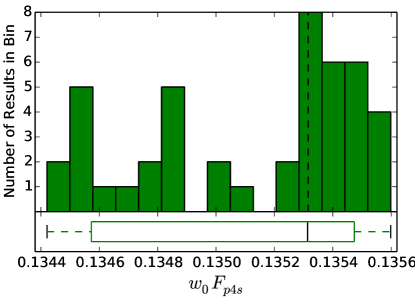
We take all the acceptable fits and create a histogram of the continuum extrapolated values. The histogram for is illustrated in Fig. 1. The histograms for both and show a bimodal distribution roughly distinguished by the presence or absence of terms. For the median and mean fall in the range where is not used, while the opposite is true for . At this time neither mode can be eliminated, so we use the full width of the entire histogram as an estimate of the systematic error from the choice of fit.


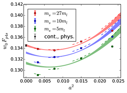
A central fit is chosen to be a fit close to the median of the distribution, with , and at least twice as many data points as parameters. For the central fit contains no terms but does contain , , and up to NNLO chiral terms. The fit has , , and passes below the physical-mass 0.06 fm ensemble. For the central fit contains , , and up to NNLO chiral terms. The fit has , , and passes below the physical-mass 0.06 fm ensemble. For both and the fm ensembles were dropped, but all values of the kaon mass were included. A plot of the central fit for is shown in Fig. 1, where is interpolated as a function of to make the plot. The accuracy of the fit can be judged using the dashed lines, which represent the fit evaluated at the same masses and lattice spacing as the data points. The three solid bands plotted across the entire figure show the lattice spacing dependence at fixed, re-tuned quark masses.
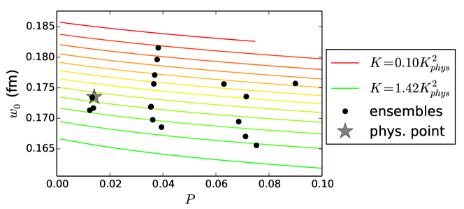
Using the central fit and data set, we determine the continuum mass dependence of . This function is useful for explicit comparisons of mass dependence to other scale setting quantities and for predicting the scales on future ensembles. The functional form of the mass dependence is chosen to be the same as the chiral perturbation theory expansion to NNLO, in agreement with the central fit. The coefficients are determined by solving the implicit equation numerically for , where the function is constructed by scaling the optimal fit by (fm) and evaluating in the continuum. Figure 2 plots this function over a large range of values for the meson masses and . Values corresponding to the HISQ ensembles and physical mass point are overlaid to give a sense of the range of data that went into constructing the plot.

4 Results and Conclusion
By evaluating and at physical quark mass, extrapolating to the continuum, and dividing by the physical value of MeV determined in Ref. [3], we compute our preliminary estimate of the gradient flow scales in physical units. The central values are taken from the center of the histograms. The first error in each case is statistical, and the remaining errors are systematic from: the choice of fit form to or (which includes continuum extrapolation and mass-interpolation errors), continuum-extrapolation and mass-interpolation errors in , residual finite volume effects on (through ), and the error in coming from the experimental error in [15].
Our results for and differ by 1.7 and 1.1 (joint) sigma, respectively, from BMW’s results, which are fm and fm [5]. HPQCD [16] used a subset of the HISQ ensembles included in our computation, but performed an independent gradient flow analysis using the Wilson action in the flow and extrapolating with instead of . Our results for and differ by 0.3 and 1.9, respectively, of the current sigma from HPQCD’s results, which are fm and fm. We do not use joint sigmas in this case because of the correlations between the two determinations. The difference with HPQCD on can be attributed largely to our inclusion of the fm ensembles in our analysis, and, to a lesser extent, our inclusion of and terms simultaneously in the continuum extrapolation. The combination of and terms are mainly needed because of the upward “hook” in the data for fm, as seen in Fig. 1.
Acknowledgments.
This work was supported by the U.S. Department of Energy and the National Science Foundation. Computations for the calculation of gradient flow were carried out with resources provided by the Texas Advanced Computing Center (TACC). The HISQ gauge configurations were generated with resources provided by the Argonne Leadership Computing Facility, the Blue Waters Project at the National Center for Supercomputing Applications (NCSA), the National Energy Resources Supercomputing Center (NERSC), the National Institute for Computational Sciences (NICS), TACC, the National Center for Atmospheric Research (UCAR), and the USQCD facilities at Fermilab, under grants from the DOE and NSF.References
-
[1]
R. Sommer, Nucl. Phys. B 411 (1994) 839 [arXiv:9310022].
-
[2]
C. Bernard et al., Phys. Rev. D 62, (2000) 034503 [arXiv:hep-lat/0002028].
-
[3]
A. Bazavov et al. [MILC Collaboration], Phys. Rev. D 90 (2014) 074509 [arXiv:1407.3772].
-
[4]
M. Lüscher, J. High Energy Phys. 1008 (2010) 071 [arXiv:1006.4518].
-
[5]
S. Borsanyi et al. [BMW], J. High Energy Phys. 1209 (2012) 010 [arXiv:1203.4469].
-
[6]
A. Bazavov et al. [MILC Collaboration], Phys. Rev. D 82 (2010) 074501 [arXiv:1004.0342].
-
[7]
A. Bazavov et al. [MILC Collaboration], Phys. Rev. D 87 (2013) 054505 [arXiv:1212.4768].
-
[8]
R. Narayanan and H. Neuberger, J. High Energy Phys. 0603 (2006) 064 [arXiv:hep-th/0601210].
-
[9]
M. Lüscher, Commun. Math. Phys. 293 (2010) 899 [arXiv:0907.5491].
-
[10]
O. Bar and M. Golterman, Phys. Rev. D 89 (2014) 034505 [arXiv:1312.4999].
-
[11]
W. Bernreuther and W. Wetzal, Nucl. Phys. B 197 (1982) 228.
-
[12]
Manohar and Wise, Heavy Quark Physics (Cambridge University Press, 2010).
-
[13]
A. Bazavov et al. [MILC Collaboration], \posPoS(Lattice 2013)269 [arXiv:1311.1474].
-
[14]
Z. Fodor et al., J. High Energy Phys. 1409 (2014) 018 [arXiv:1406.0827].
-
[15]
J. Beringer et al. [Particle Data Group], Phys. Rev. D 86 (2012) 010001.
-
[16]
R. J.Dowdall et al. [HPQCD], Phys. Rev. D 88 (2013) 074504 [arXiv:1303.1670].