SU(3) gauge theory with 12 flavours in a twisted box

Abstract:

We present preliminary result for the step-scaling study of the coupling constant with the Yang-Mills gradient flow, in the twelve-favour SU(3) gauge theory. In this work, the lattice simulation is performed using unimproved staggered fermions and the Wilson plaquette gauge action, from which the gradient flow is also implemented. Imposing twisted boundary condition a’la t’Hooft and Parisi, our calculation is performed at zero fermion mass. The renormalised coupling constant is extracted via the computation of the energy density. In order to examine the reliability of the continuum extrapolation, we investigate this coupling constant using two different lattice discretisations. Our result shows that in order to control the systematic effects in the continuum extrapolation, it is necessary to implement a large enough gradient-flow time. In the current calculation, the gauge-field averaging radius corresponding to the flow time has to be as large as $40\%$ of the lattice size.

1 Introduction

Over the past few years, there has been a significant amount of interest in identifying the minimal number of fermions, $N_{f}^{{\mathrm{cr}}}$, that results in infrared (IR) conformal behaviour of a particular gauge theory. The identification of $N_{f}^{{\mathrm{cr}}}$, which depends on the gauge group and the fermion representation, can lead to the construction of candidate models for the composite-Higgs scenario of electroweak (EW) symmetry breaking. These models can be realised using a gauge theory with the number of fermions, $N_{f}$, just below $N_{f}^{{\mathrm{cr}}}$.

Various approaches have been employed to determine $N_{f}^{{\mathrm{cr}}}$ for SU(2) and SU(3) gauge theories. In all these approaches, one has to work in the regime $N_{f}\sim N_{f}^{{\mathrm{cr}}}$. Therefore it is challenging to distinguish between the scenarios of IR conformality and chiral symmetry breaking. One of the lasting controversies in this research avenue is the IR property of SU(3) gauge theory with 12 massless flavours in the fundamental representation. While several studies led to the result that this theory can contain an infrared fixed point (IRFP) [1, 2, 3, 4, 5, 6, 7], there is evidence to support the opposite conclusion [8].

In this work, we adopt the method of step scaling [9] to investigate the behaviour of the running coupling in SU(3) gauge theory with 12 massless flavours. This method allows us to use the finite lattice size, $L$, as the renormalisation scale. The renormalisation scheme, as detailed in Sec. 2, is defined through the computation of the energy density with the implementation of the gradient flow [10, 11]. The step-scaling strategy for investigating the IR behaviour of this gauge theory requires high-precision data. This is because of the very slow running behaviour between the ultraviolet (UV) and the IR regimes. For SU(3) gauge theory with 12 massless flavours, two-loop perturbation theory predicts the existence of an IRFP at the renormalised coupling, $\bar{g}^{2}\sim 10$ ($\alpha_{s}\sim 0.8$), and

$$\left[\frac{\bar{g}^{2}(2L)}{\bar{g}^{2}(L)}\right]_{{\mathrm{two-loop}}}<1.07,$$ (1)

everywhere between the asymptotic-freedom point and the IRFP. Therefore, in numerical lattice studies, it is preferable to have data with error in the sub-percentage level, in order to obtain clear evidence for the existence/non-existence of an IRFP in this theory. Furthermore, it is also necessary to control systematic effects, which are normally dominated by the errors in the continuum extrapolation, to the same level. This task is very challenging, and was only partially achieved in previous step-scaling calculations for the running coupling in this theory [1, 3, 12]. In the present study, the statistical error of our data is well below $1\%$. We use two discretisations for computing the same renormalised coupling. This allows us to investigate the systematic error resulted from the continuum extrapolation. We find that it is necessary to implement a large enough gradient flow time (with the corresponding gauge-field averaging radius $\sim 40\%$ of the lattice size) in order to control this error.

2 Strategy and Simulation details

We adopt the Wilson plaquette gauge action and unimproved staggered fermions, with colour-twisted boundary condition [13, 14]. Details of the implementation of this boundary condition in the present calculation are exactly the same as those in Ref. [3]. In this work we use the renormalised coupling defined via the gradient flow. In particular we use the Wilson flow, defined by the equation (see Ref. [10] for any unexplained notation),

$$\frac{\partial V_{\mu}(x,t)}{\partial t}=-g_{0}^{2}\left\{\partial_{x,\mu}S_{{\mathrm{W}}}\left[V_{\mu}\right]\right\}V_{\mu}(x,t),\mbox{ }\mbox{ }V_{\mu}(x,0)=U_{\mu}(x).$$ (2)

For our step-scaling studies, we use the twisted gradient flow coupling as defined in Sec. 4 of Ref. [15],

$$\bar{g}^{2}(L)=\hat{\mathcal{N}}^{-1}(c_{\tau},a/L)\mbox{ }t^{2}\langle E(t)\rangle|_{t=c_{\tau}^{2}L^{2}/8},$$ (3)

where

$$E(t)=-\frac{1}{2}{\rm tr}\left(G_{\mu\nu}G_{\mu\nu}\right)$$ (4)

is the energy density at positive flow time, $G_{\mu\nu}$ is the field strength tensor, and $c_{\tau}$ is a dimensionless parameter that characterises our scheme. Finally $\hat{\mathcal{N}}(c_{\tau},a/L)$ ensures that at leading order our coupling is the same as the coupling in the $\overline{{\mathrm{MS}}}$ scheme. We note that $\hat{{\mathcal{N}}}(c_{\tau},a/L)$ is computed on the lattice, and therefore our coupling definition does not contain any leading order lattice artefacts. It is alo free from the zero-mode contribution because of the use of twisted boundary condition.

Similar definitions of the renormalised coupling have been investigated in Refs. [7, 11, 15, 16, 17]. In these previous works, it was observed that the statistical error of $\bar{g}^{2}$ are significantly smaller than that in other methods, such as the twisted Polyakov loop scheme [18]. This is also what we find in this work, where we compute the coupling every 50 to 200 Hybrid Monte-Carlo trajectories.

To implement the step-scaling approach, we perform simulations on lattices with the choices of volume,

$$\hat{L}\equiv L/a=6,8,10,12,16,20,24,$$ (5)

at many values of the lattice spacing, $a$. The Wilson flow, as described in Eq. (2), can be shown to result in the average of the gauge potential in the 4-dimensional sphere with mean-square radius $\sqrt{8t}$. This introduces a scale,

$$\mu=\frac{1}{\sqrt{8t}},$$ (6)

in the extraction of the coupling in Eq. (3). Therefore, to implement the step-scaling method, we have to ensure that the ratio,

$$c_{\tau}\equiv\frac{\sqrt{8t}}{L}=\frac{1}{\mu L},$$ (7)

is fixed in the procedure. This leads to the definition of a coupling, through Eq. (3), at the renormalisation scale $L$. In the rest of this article, we will denote this coupling as $\bar{g}(L)$. From the above discussion, it is obvious that $c_{\tau}$ should be larger than 0 and smaller than 0.5. Picking a value of $c_{\tau}$ corresponds to specifying a renormalisation scheme.

Tuning the bare couplings on the lattice sizes $\hat{L}=6,8,10,12$, such that the renormalised couplings are identical, we can make certain that these lattices are of the same physical size, $L$. Using these tuned bare couplings (lattice spacings), we then compute the renormalised coupling on the lattices that are twice larger. That is, we perform the calculation at $\hat{L}=12,16,20,24$ at these lattice spacings. This allows us to carry out the continuum extrapolation for the coupling renormalised at $2L$.

3 Analysis and Results

It is well known that the main source of the systematic effects in the step-scaling method is the lattice artefacts. In this work, we use two lattice discretisations, namely the clover operator and the plaquette, to compute the energy density in extracting the coupling defined in Eq. (3). We denote the “lattice version” of the renormalised coupling generically as $\bar{g}^{2}_{{\rm latt}}$. By comparing results from these two discretisations, we can investigate the effect of the lattice artefacts and the reliability of the continuum extrapolation. Furthermore, we calculate $\bar{g}^{2}_{{\rm latt}}$ at many values of $c_{\tau}$ between 0 and 0.5. This allows us to study the effect of $c_{\tau}$ on the size of the discretisation error.

Figure 1: Examples of interpolation in the bare coupling in this work.

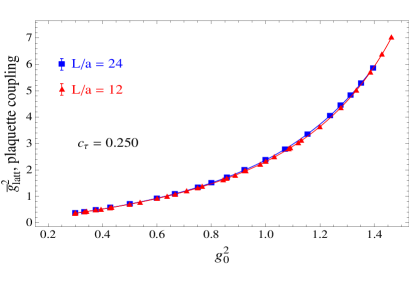
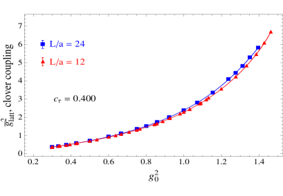
The implementation of the step-scaling approach involves careful tuning of the bare coupling, in order to set up the constant physical size of the lattice. In practice, we carry out this tuning procedure by computing the renormalised coupling with many values of the bare coupling, for each lattice volume in Eq. (5). At each choice of $\hat{L}$, through interpolation, we can then determine $\bar{g}^{2}_{{\rm latt}}$ as a function of $g^{2}_{0}$ within the interval where we have data. This interpolation is performed using a non-decreasing function proposed in Sec. V.B of Ref. [3]. Figure 1 demonstrates the result of such interpolations for $\hat{L}=12$ and 24, at two choices of $c_{\tau}$ for both the clover and the plaquette discretisations. In the upper right panel, the plot shows the “crossing” phenomenon, which means $\bar{g}^{2}_{{\rm latt}}$ decreases when $\hat{L}$ is increased at fixed bare coupling constant, in the strong-coupling regime. In the current work, this phenomenon happens for $\bar{g}^{2}_{{\rm latt}}$ computed using the plaquette discretisation at $c_{\tau}\leq 0.45$. We have not observed it with the clover discretisation.

Figure 2: Examples of continuum extrapolation, using a linear function in $(a/L)^{2}$ and data from the 3 finest lattices in each case. In the upper-right panel, the result for $\bar{g}^{2}_{{\rm latt}}(2L)$ from the clover discretisation on the coarsest lattice is $\sim 6.5$, and is off the range of this plot. The extrapolated results for the plaquette discretisation are shifted for clarity.

Once we have performed the bare-coupling interpolation for $\bar{g}^{2}_{{\rm latt}}$, it is straightforward to determine the values of $g^{2}_{0}$ which lead to

$$\bar{g}^{2}(L)=\bar{g}^{2}_{{\rm latt}}(6\times a_{6})=\bar{g}^{2}_{{\rm latt}}(8\times a_{8})=\bar{g}^{2}_{{\rm latt}}(10\times a_{10})=\bar{g}^{2}_{{\rm latt}}(12\times a_{12}),$$ (8)

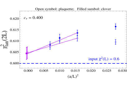
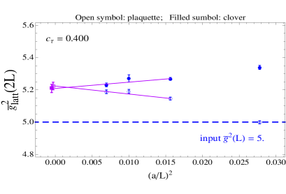
where $a_{6,8,10,12}$ are the lattice spacings for the lattices with sizes, $\hat{L}=6,8,10,12$. This can be done at any $\bar{g}^{2}$ in the range where we have data. The next step is to adopt these tuned $a_{6,8,10,12}$, and perform the continuum extrapolation using $\bar{g}^{2}_{{\rm latt}}(12\times a_{6})$, $\bar{g}^{2}_{{\rm latt}}(16\times a_{8})$, $\bar{g}^{2}_{{\rm latt}}(20\times a_{10})$, and $\bar{g}^{2}_{{\rm latt}}(24\times a_{12})$. This enables us to determine $\bar{g}^{2}(2L)$ for a given value of $\bar{g}^{2}(L)$. It is well known that this extrapolation procedure is the main source of the systematic error in the step-scaling study of the coupling constant. This is also the case in our current work. We first notice that our coarsest lattice contains significant lattice artefacts effect. Therefore we do not use data with $(\hat{L}=6\rightarrow\hat{L}=12)$ in the continuum extrapolation. This means we carry out a linear fit in $(a/L)^{2}$ with the data,

$$\left(\hat{L}=8\rightarrow\hat{L}=16,\mbox{ }\hat{L}=10\rightarrow\hat{L}=20,\mbox{ }\hat{L}=12\rightarrow\hat{L}=24\right),$$ (9)

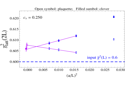
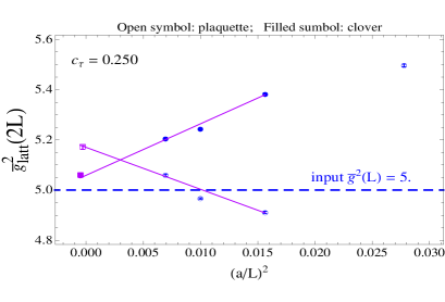
for this procedure. In Fig. 2, we show examples of the continuum extrapolation with two choices of $c_{\tau}$. As expected, increasing $c_{\tau}$ leads to smaller effects of the lattice artefacts. The cases with $c_{\tau}=0.25$ in the figure show that the plaquette and the clover discretisations of the same Yang-Mills field tensor give different results in the continuum limit, although the individual extrapolation seems acceptable. This feature becomes conspicuous in the strong coupling regime (the upper-right panel of Fig. 2). Therefore, we conclude that the continuum extrapolation is not under control at $c_{\tau}=0.25$. In fact, we find that it is necessary to increase $c_{\tau}$ to be $\sim 0.4$, in order to have reliable results in the continuum limit. This is demonstrated in the two lower panels in Fig. 2.

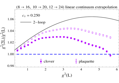
Figure 3 displays our results for $\bar{g}^{2}(2L)/\bar{g}^{2}(L)$, plotted against the input $\bar{g}^{2}(L)$. The left panel contains results obtained using the clover and the plaquette discretisations at $c_{\tau}=0.25$. This plot shows the importance of investigating the systematic effect in the continuum extrapolation. It demonstrates that the systematic error in the strong coupling regime is large for the case $c_{\tau}=0.25$, such that we cannot draw any conclusion regarding the existence of the IRFP.

Figure 3: Results of the step-scaling. These plots indicate that the clover and plaquette discretisations give consistent continuum-limit result only at large enough $c_{\tau}$. Working with a small value of $c_{\tau}$ and only one discretisation method may lead to incorrect conclusion regarding the existence of the IRFP.

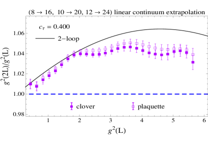
The right panel of Fig. 3 indicates that in the range of the coupling that we have studied, it is enough to work with the choice $c_{\tau}=0.4$ to control the continuum extrapolation. Of course, this still has to be confirmed with further investigation. Presently we are generating data at one lattice spacing with $\hat{L}=32$ in the strong-coupling regime, and use it to examine the reliability of our results in the continuum limit.

4 Conclusion and Outlook

In this article, we present preliminary results of our step-scaling study of the running coupling in SU(3) gauge theory with 12 massless flavours. We use the renormalised coupling extracted from the energy density at positive gradient-flow time with twisted boundary conditions. This renormalisation scheme enables us to have data with statistical errors at the sub-percentage level. Such accuracy is essential in the investigation of the IR behaviour of this theory, in which the coupling runs very slowly.

We find that cutoff effect in the gradient flow scheme can be difficult to control. To study this systematic effect, we use two discretisations to define the coupling. We find that continuum extrapolations agree for both discretisations only at large values of the flow time ($c_{\tau}\sim 0.4$). With various newly-proposed techniques [19, 20] relevant to improving the Wilson flow, one may be able to work with a smaller $c_{\tau}$. We will study some of these methods in the future.

Presently we are performing lattice simulations in the regime of stronger couplings. We envisage that it is possible to have data up to $\bar{g}\sim 6.3$ in our work, with simulations still performed on the weak-coupling side of the bulk phase structure in the lattice theory [21, 22]. It is desirable that our work will shed light on the controversy over the existence of the IRFP in SU(3) gauge theory with 12 massless flavours.