Symmetric low-rank representation for subspace clustering
Abstract
We propose a symmetric low-rank representation (SLRR) method for subspace clustering, which assumes that a data set is approximately drawn from the union of multiple subspaces. The proposed technique can reveal the membership of multiple subspaces through the self-expressiveness property of the data. In particular, the SLRR method considers a collaborative representation combined with low-rank matrix recovery techniques as a low-rank representation to learn a symmetric low-rank representation, which preserves the subspace structures of high-dimensional data. In contrast to performing iterative singular value decomposition in some existing low-rank representation based algorithms, the symmetric low-rank representation in the SLRR method can be calculated as a closed form solution by solving the symmetric low-rank optimization problem. By making use of the angular information of the principal directions of the symmetric low-rank representation, an affinity graph matrix is constructed for spectral clustering. Extensive experimental results show that it outperforms state-of-the-art subspace clustering algorithms.
keywords:
Subspace clustering , spectral clustering , symmetric low-rank representation , affinity matrix , low-rank matrix recovery , dimension reduction1 Introduction
Subspace clustering is one of the fundamental topics in machine learning, computer vision, and pattern recognition, e.g., image representation [1, 2], face clustering [3, 4, 2], and motion segmentation [5, 6, 7, 8, 9]. The importance of subspace clustering is evident in the vast amount of literature thereon, because it is a crucial step in inferring structure information of data from subspaces through data analysis [10, 11, 12]. Subspace clustering refers to the problem of clustering samples drawn from the union of low-dimensional subspaces, into their subspaces.
When considering subspace clustering in various applications, several types of available visual data are high-dimensional, such as digital images, video surveillance, and traffic monitoring. These high-dimensional data often have a small intrinsic dimension, which is often much smaller than the dimension of the ambient space. For instance, face images of a subject, handwritten images of a digit with different rotations, and feature trajectories of a moving object in a video often lie in a low-dimensional subspace of the ambient space [13, 14]. To describe a given collection of data well, a more general model is to consider data drawn from the union of low-dimensional subspaces instead of a single lower-dimensional subspace [2, 15].
Subspace clustering has been studied extensively over several decades. A number of techniques for exploiting low-dimensional structures of high-dimensional data have been proposed to tackle subspace clustering. Based on their underlying techniques, subspace clustering methods can be roughly divided into four categories according to the mechanism used: algebraic [16], statistical [17], iterative [18], and spectral clustering based methods [2, 19, 20, 21, 4]. For a more detailed explanation of these algorithms, we refer the reader to [10], which contains a recent review.
If there are no errors in the data, i.e., the data are strictly drawn from multiple subspaces, several existing methods can be used to solve subspace clustering exactly [22, 23, 2, 4]. However, the assumption of low-dimensional intrinsic structures of data is often violated when the real observations are contaminated by noise and gross corruption. Consequently, this results in inferior performance. A number of research efforts have focused on these problems. Spectral clustering based methods, such as sparse representation [4], low-rank representation [2], and their extensions [19, 24, 20, 25, 26] have yielded excellent performance in exploiting low-dimensional structures of high-dimensional data. Most existing methods perform subspace clustering involving two steps: first, learning an affinity matrix that encodes the subspace memberships of samples, and then obtaining the final clustering results with the learned affinity matrix using spectral clustering algorithms such as normalized cuts (NCuts) [27, 28]. The fundamental problem is how to build a good affinity matrix in these steps.
Inspired by recent advances in -norm and -norm techniques [29, 30, 31], the introduction of sparse representation based techniques has resulted in enhanced separation ability in subspace clustering. Elhamifar and Vidal [4] proposed a sparse subspace clustering (SSC) algorithm to cluster data points lying in the union of low-dimensional subspaces. SSC considers that each data point can be represented as a sparse linear combination of other points by solving an -norm minimization problem. The -norm minimization program can be solved efficiently using convex programming tools. If the subspaces are either independent or disjoint under the appropriate conditions, SSC succeeds in recovering the desired sparse representations. After obtaining the desired sparse representation to define an affinity matrix, spectral clustering techniques are used to obtain the final clustering results. SSC shows very promising results in practice. Nasihatkon and Hartley [32] further analyzed connectivity within each subspace based on the connection between the sparse representations through -norm minimization. Wang and Xu [33] extended SSC by adding either adversarial or random noise to study the behavior of sparse subspace clustering. However, some critical problems remain unsolved. In particular, the above techniques find the sparsest representation of each sample individually, which leads to high computational cost. Besides, a global structural constraint on the sparse representation is lacking, i.e., there is no theoretical guarantee that the nonzero coefficients correspond to points in the same subspace in the presence of corrupted data.
Low-rank representation based techniques have been proposed to address these drawbacks [2, 34, 9]. Liu et al. [2] proposed the low-rank representation (LRR) method to learn a low-rank representation of data by capturing the global structure of the data. The LRR method essentially requires singular value decomposition (SVD) at each iteration and needs hundreds of iterations before convergence. The computational complexity of LRR becomes computationally impracticable if the dimensionality of the samples is extremely large. Although an inexact variation of the augmented Lagrange multiplier (ALM) method [35, 36], which is used to solve the optimization problem in LRR, performs well, and generally converges adequately in many practical applications, its convergence property still lacks a theoretical guarantee. Vidala and Favarob [9] considered low-rank subspace clustering (LRSC) as a non-convex matrix decomposition problem, which can be solved in closed form using SVD of the noisy data matrix. Although LRSC can be carried out on data contaminated by noise with reduced computational cost, the clustering performance could be seriously degraded owing to the presence of such corrupted data. Chen and Yi [37] presented a low-rank representation with symmetric constraints (LRRSC) method. LRRSC further exploits the angular information of the principal directions of the symmetric low-rank representation for improved performance. However, LRRSC cannot avoid iterative SVD computations either, which is still time consuming. Consequently, LRRSC suffers from heavy computational cost when computing a symmetric low-rank representation. To obtain a good affinity matrix for spectral clustering using low-rank representation techniques, which can lead to higher performance and lower computational cost, low-rank representation of high-dimensional data still deserves investigation.
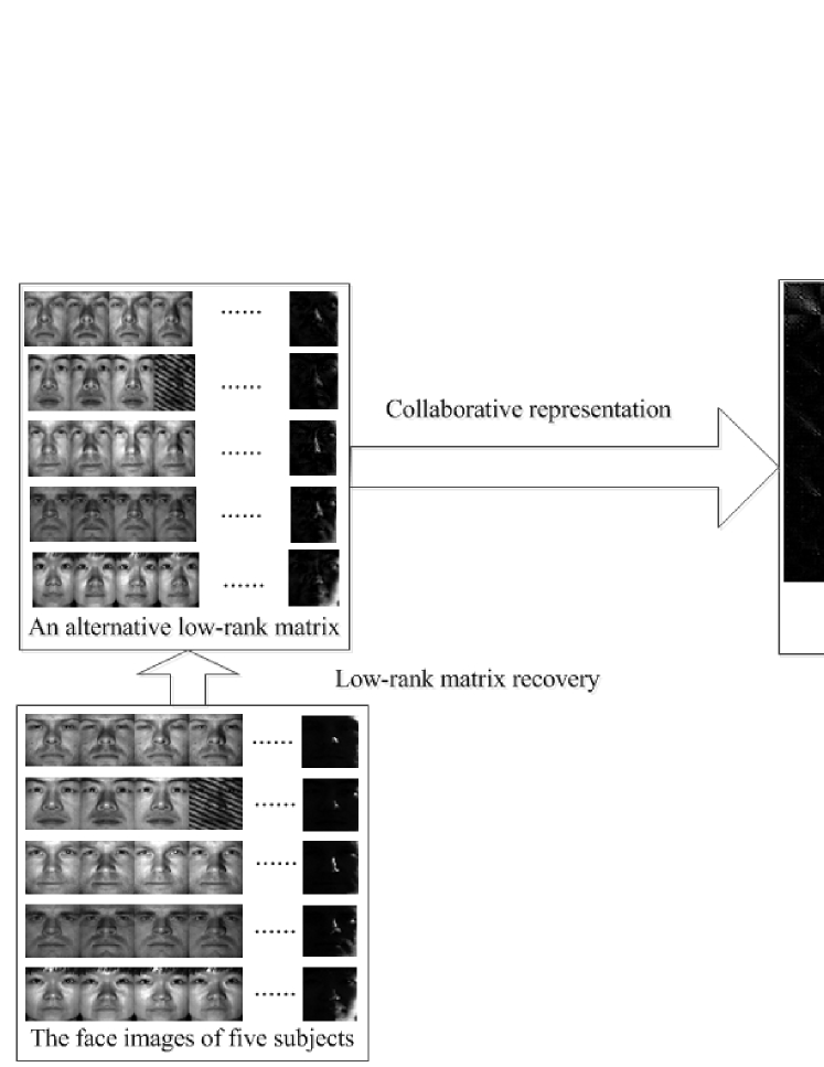
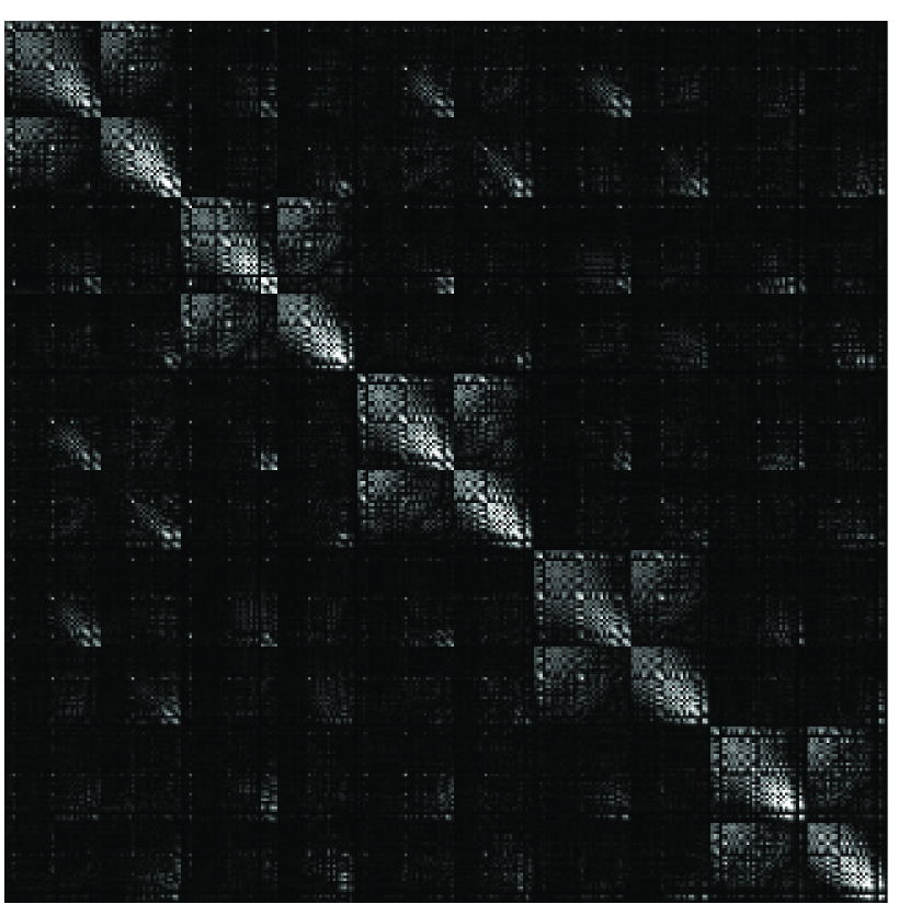
In this paper, we address the problem of subspace clustering by introducing the symmetric low-rank representation (SLRR) method. SLRR can be regarded as an improvement of our previous work, i.e., LRRSC [37]. Figure 1 shows an intuitive clustering example using five subjects to illustrate our approach. Owing to the self-expressiveness property of the data, our motivation starts from an observation of collaborative representation, which plays an important role in classification and clustering tasks [38, 39]. In particular, our motivation is to integrate the collaborative representation combined with low-rank matrix recovery techniques into a low-rank representation to learn a symmetric low-rank representation. The representation matrix involves the symmetric and low-rankness property of high-dimensional data representation, thereby preserving the low-dimensional subspace structures of high-dimensional data. An alternative low-rank matrix can be obtained by making use of the low-rank matrix recovery techniques closely related to the specific clustering problems. In contrast with -norm minimization or iterative shrinkage, SLRR obtains a symmetric low-rank representation in a closed form solution by solving the symmetric low-rank optimization problem. Thereafter, an affinity graph matrix can be constructed by computing the angular information of the principal directions of the symmetric low-rank representation for spectral clustering. Further details are discussed in Section 3.
The proposed SLRR method has several advantages:
-
1.
It incorporates collaborative representation combined with low-rank matrix recovery techniques into a low-rank representation, and can successfully learn a symmetric low-rank representation, which preserves the multiple subspace structure, for subspace clustering.
-
2.
A symmetric low-rank representation can be obtained in a closed form solution by the symmetric low-rank optimization problem, which is similar to solve a regularized least squares regression. Consequently, it avoids iterative SVD operations, and can be employed by large-scale subspace clustering problems with the advantages of computational stability and efficiency.
-
3.
Compared with state-of-the-art methods, our experimental results using benchmark databases demonstrate that the proposed method not only achieves competitive performance, but also dramatically reduces computational cost.
The remainder of the paper is organized as follows. A brief overview of some existing work on rank minimization is given in Section 2. Section 3 provides a detailed description of the proposed SLRR for subspace clustering. Section 4 presents the experiments to evaluate the proposed SLRR on benchmark databases. Finally, Section 5 concludes the paper.
2 Review of previous work
Let be a set of -dimensional data vectors drawn from the union of subspaces of unknown dimensions. Without loss of generality, we can assume , where consists of the vectors of . The task of subspace clustering involves clustering data vectors into the underlying subspaces. This section provides a review of low-rank representation techniques for subspace clustering.
Liu et al. [2] proposed the LRR method for subspace clustering. In the absence of noise, LRR solves the following rank minimization problem:
| (1) |
where is an overcomplete dictionary. Since problem (1) is non-convex and NP-hard, LRR uses the nuclear norm as a common surrogate for the rank function:
| (2) |
where denotes the nuclear norm (that is, the sum of the singular values in the matrix).
In the case of data grossly corrupted by noise or outliers, LRR solves the following convex optimization problem:
| (3) |
where is a parameter to balance the effects of the low-rank representation and errors, and indicates a certain regularization strategy for characterizing various corruptions. For instance, the -norm characterizes the error term that encourages the columns of error matrix to be zero. LRR uses the actual data as the dictionary. The above optimization problem can be efficiently solved by the inexact augmented Lagrange multipliers (ALM) method [35]. A post-processing step involves using to construct the affinity matrix as , which is symmetric and entrywise nonnegative. The final data clustering result is obtained by applying spectral clustering to the affinity matrix.
3 Symmetric low-rank representation
In this section, we discuss the core of the proposed method, which is to learn a SLRR for subspace clustering. The SLRR was inspired by collaborative representation and low-rank representation techniques, which are used in classification and subspace clustering [2, 38, 39]. This proposed technique identifies clusters using the angular information of the principal directions of the symmetric low-rank representation, which preserves the low-rank subspace structures. In particular, we first analyze the symmetric low-rank property of high-dimensional data representation based on the symmetric low-rank optimization problem, which is closely related with the regularized least squares regression. Then, we attempt to find an alternative low-rank matrix instead of the original data combined with low-rank matrix recovery techniques to obtain a symmetric low-rank representation. We further give the equivalence analysis of optimal solutions between problem (5) and (8). Finally, we construct the affinity graph matrix for spectral clustering, which completes the procedure for the SLRR method.
3.1 The symmetric low-rank representation model
In the absence of noise, i.e., the samples are strictly drawn from multiple subspaces, several criteria are imposed on the optimization models to learn the representation of samples as an affinity matrix for spectral clustering to solve the subspace clustering problem exactly [4, 2, 40, 39]. For example, SSC employs the sparsest representation using an -norm regularization, while LRR seeks to learn the lowest-rank representation using a nuclear-norm regularization. Both of these techniques can realize an affinity matrix of the samples involving the block diagonal between-clusters property, which reveals the membership of subspaces with theoretical guarantees. By considering noise and corruption in real observations, the lowest-rank criterion shows promising robustness among these criteria by capturing the global structure of the samples.
As mentioned above, the lowest-rank criterion, such as LRR, typically requires calculating singular value decomposition iteratively. This means that it becomes inapplicable both in terms of computational complexity and memory storage when the dimensionality of the samples is extremely large. To alleviate these problems, we design a new criterion as the convex surrogate of the nuclear norm. It is worth noting that we are intersected in a symmetric low-rank representation of a given data set. But we are not interested in seeking the best low-rank matrix recovery and completion using the obtained symmetric low-rank representation. The proposed method differs from the LRR method in terms of its matrix recovery. In the case of noisy and corrupted data, we seek to find a symmetric low-rank representation using collaborative representation combined low-rank representation techniques. The optimization problem is as follows:
| (4) |
The discrete nature of the rank function makes it difficult to solve Problem (4). Many researchers have instead used the nuclear norm to relax the optimization problem [2, 19, 19, 37]. Unfortunately, these methods cannot completely avoid the need for iterative singular value decomposition (SVD) operations, which incur a significant computational cost. Unlike these LRR-based methods that solve the nuclear norm problem, the following convex optimization provides a good surrogate for problem (4):
| (5) |
where denotes the Frobenius norm of the matrix, is a parameter used to balance the effects of the two parts, and is a parameter used to guarantee the low-rank representation . To maintain the weight consistency of each pair of data points, we impose a symmetric constraint on representation . Then, by imposing a low-rank constraint on representation , we obtain a desired symmetric low-rank representation.
To further analyze problem (5), we first simplify this optimization problem. Removing the constraint from the problem leads to another optimization problem:
| (6) |
The solution of SLRR in problem (6) can be analytically obtained
| (7) |
where is the identity matrix, and is a parameter.
Next, we show that is symmetric.
Theorem 1.
The matrix
is symmetric.
Proof.
Clearly,
On the other hand,
Since , is symmetric. ∎
It should be pointed out that may not be a low-rank matrix. Denote the ranks of and by and , respectively. It is easy to see that . As the noises we confront are ubiquitous in practice, is not a low-rank matrix. This implies that the real data may not strictly follow subspace structures because of noise or corruption.
In general, is a low-rank matrix if is low-rank. If we require that , where is some small positive integer, then is a symmetric low-rank matrix. If we can use an alternative low-rank matrix to replace , a desired low-rank solution could be obtained. We propose the following convex optimization provides a good surrogate for the problem (5).
| (8) |
If , then
| (9) |
is the analytical optimal solution to problem (8).
From linear algebra, is a symmetric low-rank matrix if is low-rank. The only remaining issue is how to get an alternative low-rank matrix instead of from a given set of data.
3.2 Pursuing an alternative low-rank matrix through low-rank matrix recovery techniques
Given the assumption mentioned above, data points are approximately drawn from a union of subspaces. Each data point can be represented by a linear combination of the other data points. Therefore, it is reasonable that a low-rank matrix recovered from corrupt observations is employed instead of the original data in problem (6). Here we consider in detail, three implementations of an alternative low-rank matrix from corrupt observations.
First, we explain the idea behind the first implementation. We incorporate low-rank matrix recovery techniques, the choice of which is closely related to the specific problem, into recovering corrupt samples. For example, it is well known that principal component analysis (PCA) is one of the most popular dimension reduction techniques for face images [41]. PCA assumes that the data is drawn from a single low-dimensional subspace. In fact, our experiments demonstrate its effectiveness when applied to face clustering and motion segmentation. In particular, PCA learns a low-rank project matrix by minimizing the following problem:
| (10) |
Let . Note that is low-rank matrix recovery of . If , a globally optimal solution of problem (8) can be obtained in closed form. Obviously, it is a symmetric low-rank matrix. The low-rank matrix recovery reveals its vital importance in learning a low-rank representation.
It is well known that PCA is an effective method when the data are corrupted by Gaussian noise. However, its performance is limited in real applications by a lack of robustness to gross errors. The second implication for consideration is to recover a low-rank matrix from highly corrupted observations. For example, RPCA decomposes the data matrix into the sum of a low-rank approximation and an additive error [42, 43], which leads to the following convex problem:
| (11) |
Assume that the optimal solution to this problem is , where , where is a low-rank matrix. If , a globally optimal solution can be obtained for problem (8).
Besides, we further consider incorporating feature extraction into the low-rank representation. We use low-rank features extracted from the corrupted samples instead of the original data by dimension reduction techniques. We also use the face clustering example to illustrate the importance and feasibility of feature extraction. Random features can be viewed as a less-structured face feature. Randomfaces are independent of the face images [44, 45]. A low-rank transform matrix , whose entries are independently sampled from a zero-mean normal distribution, is extremely efficient to generate, whose entries are independently sampled from zero-mean normal distribution. The random project (RP) matrix can be used to for dimension reduction for of face images. Let , where is an extracted feature matrix. A globally optimal solution to problem (8) can also be obtained.
To examine the connection among the low-rank matrix recovery techniques reliant on dimension reduction, we consider the special case in which the low-rank projection matrix has orthogonal columns, i.e., . Assuming that , both of the implications, i.e., and , are equivalent to each other in problem (8). This is summarized by the following Lemma.
Lemma 1.
Let , , and be matrices of compatible dimensions. Suppose and have orthogonal columns, i.e., and , then we have
Proof.
By definition of the Frobenius norm, we have
As and , we have
∎
According to Lemma 1, we can conclude that , where the low-rank project matrix has orthogonal columns. Consequently, or are alternatives to obtain the same globally optimal solution of problem (8). The computational cost of the first implementation can be effectively reduced by using a simplified version if the low-rank project matrix has orthogonal columns.
The use of low-rank matrix recovery techniques to improve the performance of many applications is not in itself surprising. However, in this paper, the main purpose of using such techniques is to derive an alternative low-rank matrix that can be used to obtain the symmetric low-rank representation discussed above.
3.3 Equivalence analysis of optimal solutions
In Section 3.1, we first introduced problem (5) to describe a symmetric low-rank representation model, and then considered this problem as the surrogate of an alternative low-rank matrix. We then analyzed the equivalence between problems (5) and (8) in terms of the optimal solution.
Let us first consider a specific case of low-rank matrix recovery techniques, such as PCA . In PCA, the low-rank projection matrix is an orthogonal matrix, i.e., . Then, problem (5) can be converted into an equivalent problem (8) according to Lemma 1. Consequently, the globally optimal solution of problem (8), , is the same as that of problem (5). It is clear that is a symmetric low-rank representation that preserves the multiple subspace structure.
Furthermore, we note the remaining cases of low-rank matrix recovery techniques, such as RP and RPCA . For example, the columns of the low-rank projection matrix may not be orthogonal to one another, or an alternative low-rank matrix recovered from the original data may not be directly obtained using the low-rank projection matrix. Thus, we cannot calculate the globally optimal solution of problem (5) directly since its solution is intractable. To address this problem, we integrate an alternative low-rank matrix into problem (8) to learn a symmetric low-rank representation. As mentioned above, problem (8) can be solved as a closed form solution. It should be emphasized that this surrogate is reasonable for the following two reasons: (1) high-dimensional data often lie close to low-dimensional structures; and (2) the alternative matrix recovered from the original data has low rank. Such a symmetric low-rank representation can also preserve the multiple subspace structure.
3.4 Construction of an affinity graph matrix for subspace clustering
Using the symmetric low-rank matrix from problem (8), we need to construct an affinity graph matrix . We consider with the skinny SVD , and define . As suggested in [37], we apply the mechanism of driving the construction of the affinity graph from matrix . This considers the angular information from all row vectors of matrix or all column vectors of matrix to define an affinity graph matrix as follows:
| (12) |
where and represent the -th and -th rows of matrix , and and represent the -th and -th columns of matrix , respectively, and is a parameter to adjust the sharpness of the affinity between different clusters. Algorithm 1 summarizes the complete subspace clustering algorithm for SLRR.
Assume that the size of is , where has samples and each sample has dimensions. For convenience, we apply PCA as an example low-rank matrix recovery technique to illustrate the computational complexity of Algorithm 1. Thus, the computational complexity of the first two steps in Algorithm 1 is , while the computational complexity of the last four steps in Algorithm 1 is . The complexity of Algorithm 1 is . If , the overall complexity of Algorithm 1 is .
4 Experiments
4.1 Experimental settings


4.1.1 Databases
To evaluate the SLRR, we performed different experiments on two popular benchmark databases, e.g., the extended Yale B and Hopkins 155 databases. The statistics of the two databases are summarized below.
-
1.
Extended Yale B database [46, 47]. This database contains 2414 frontal images of 38 individuals, with images of each individual lying in a low-dimensional subspace. There are around images available for each individual. To reduce the computational time and memory requirements of algorithms, we used a normalized face image with size pixels in the experiments. Figure 2(a) shows some example face images from the Extended Yale B Database.
-
2.
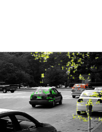
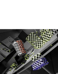
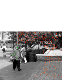
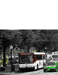
Hopkins 155 database [48]. This database consists of 156 video sequences of two or three motions. Each video sequence motion corresponds to a low-dimensional subspace. There are data vectors drawn from two or three motions for each video sequence. Figure 7 shows some example frames from four video sequences with traced feature points.
4.1.2 Baselines and evaluation
To investigate the efficiency and robustness of the proposed method, we compared the performance of SLRR with several state-of-the-art subspace clustering algorithms, such as LRR [2], LRRSC [37], SSC [4], local subspace affinity (LSA) [49], and low rank subspace clustering (LRSC) [9]. For the state-of-the-art algorithms, we used the source code provided by the respective authors. The Matlab source code for our method is available online at http://www.machineilab.org/users/chenjie.
The subspace clustering error is the percentage of misclassified samples over all samples, which is measured as
| (13) |
where denotes the number of misclassified samples, and is the total number of samples. For LRR, we reported the results after post-processing of the affinity graph. Moreover, we chose the noisy data version of of LRSC to show its results. All experiments were implemented on Matlab R2011b and performed on a personal computer with an Intel Core i5-2300 CPU and 16 GB memory.
4.1.3 Parameter settings
| Method | Face clustering | |
|---|---|---|
| Scenario 1 | Scenario 2 | |
| SLRRPCA | ||
| SLRRRP | ||
| SLRRRPCA | - | |
| LRRSC | ||
| LRR | ||
| SSC | ||
| LSA | ||
| LRSC | ||
| Method | Motion segmentation | |
|---|---|---|
| Scenario 1 | Scenario 2 | |
| SLRR | ||
| LRRSC | ||
| LRR | ||
| SSC | ||
| LSA | ||
| LRSC | ||
To obtain the best results of the state-of-the-art algorithms in the experiments, we either applied the optimal parameters for each method as given by the respective authors, or manually tuned the parameters of each method. We emphasize that SLRR is follow-up research based on our previous work, i.e., LRRSC [37]. Hence, we reported the parameter settings and results of several algorithms from [37], e.g., LRR, LRRSC, SSC, LSA and LRSC, for comparison with the results of SLRR in our experiments. The parameters for these methods are set as shown in Tables 1 and 2.
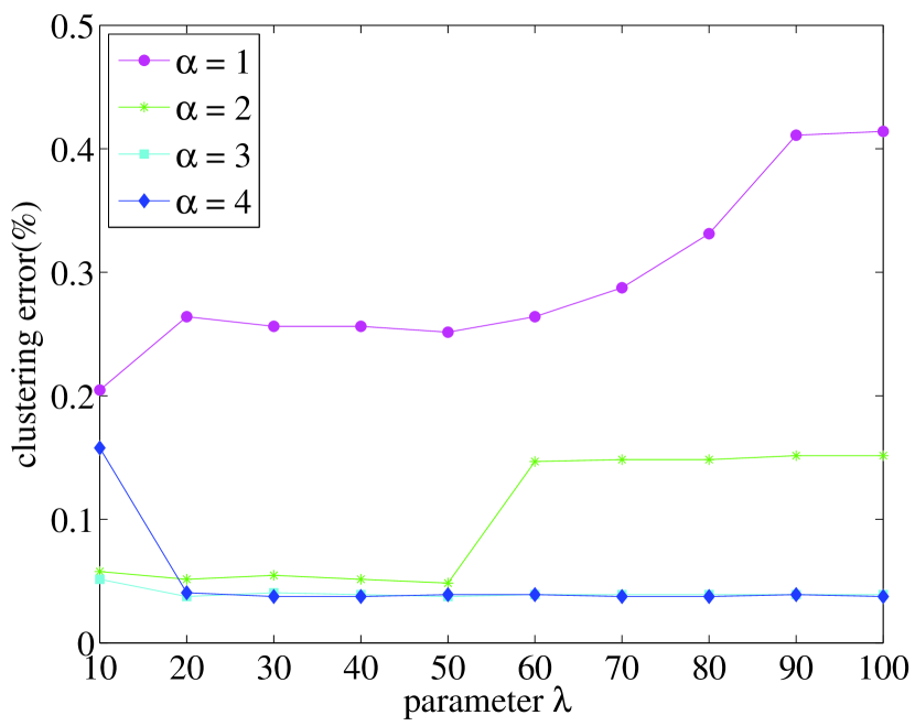
According to problem (8), SLRR has three parameters: , and . Empirically speaking, parameter should be relatively large if the data are slightly contaminated by noise, and vice versa. In other words, parameter is usually dependent on the prior of the error level of data. In fact, parameter has a wide range in our experiments. Parameter ranges from 2 to 4. To pursue an alternative low-rank matrix, parameter may be closely related with the intrinsic dimension of high-dimensional data. For example, images of an individual with a fixed pose and varying illumination lie close to a 9-dimensional linear subspace under the Lambertian assumption [14]. Besides, the tracked feature point trajectories from a single motion lie in a linear subspace of at most four dimensions [13]. Therefore, we used in some face clustering experiments shown in Table 1, and for the motion segmentation experiments shown in Table 2, where denotes the number of subspaces. Note that we used in SLRRPCA for the first scenario of face clustering. However, using for SLRRPCA also achieves satisfactory performance in the face clustering experiments. Further results and discussions of the parameters are given in the respective sections for the experiments.
4.2 Experiments on face clustering
We first evaluated the clustering performance of SLRR as well as the other methods on the Extended Yale B database. Face clustering refers to the problem of clustering face images from multiple individuals according to each individual. The face images of the individual, captured under various laboratory-controlled lighting conditions, can be well approximated by a low-dimensional subspace [14]. Therefore, the problem of clustering face images reduces to clustering a collection of images according to multiple subspaces. We considered two different clustering scenarios of face images to evaluate the performance of the proposed SLRR.
4.2.1 First scenario for face clustering
Following the experimental settings in [3], we chose a subset of the Extended Yale B database consisting of the 640 frontal face images from the first 10 subjects. We used two different low-rank matrix recovery techniques (PCA, RPCA) and one dimension reduction technique (RP) to implement SLRR for face clustering.
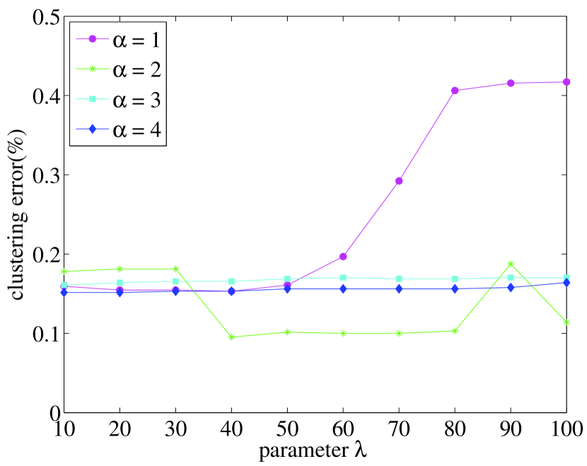
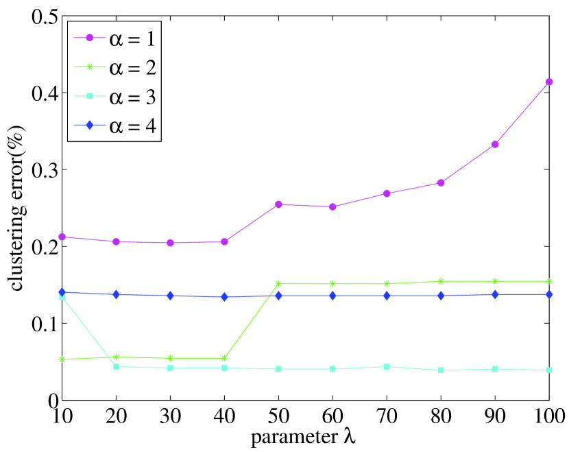
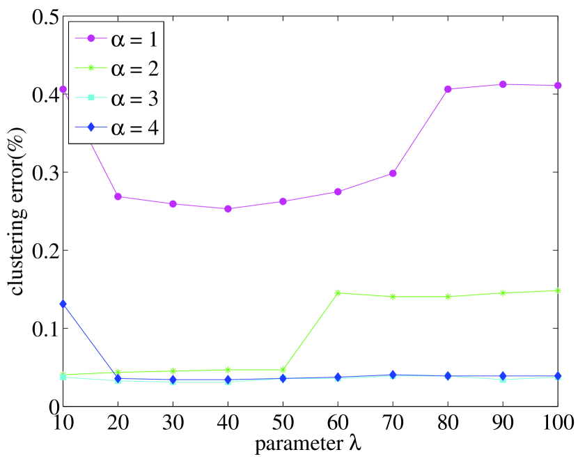
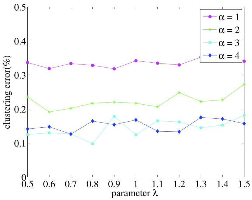
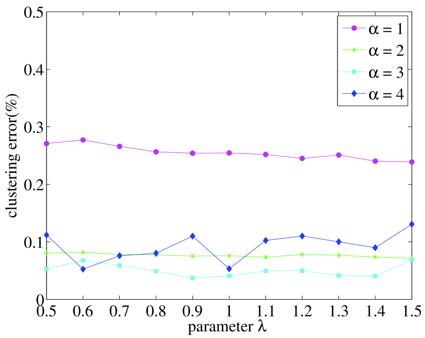
We first examined the performance of these algorithms on the original data. Figures 3 and 4 show the influence of parameters and for different values on the clustering errors of SLRR. Note that is the value of the reduced dimension after applying PCA or RP. Because the random projection matrix used in SLRRRP is generated randomly, ten different random projection matrices are employed in the performance evaluation. The final clustering performance of SLRRRP is computed by averaging the clustering error rates from these ten experiments. According to the Lambertian assumption mentioned above, the optimal value of is around 90 because of the 10 different subjects in the experiment. As shown in Figs. 3(a) and 4(a), a value of equal to results in inferior clustering performance. This implies that the reduced dimension information of face images, whose dimension is much less than the intrinsic dimension of face images, is not sufficient for low-rank representation to separate data from different subspaces. In contrast to the reduced dimension of the face images, a value of equal to or greater than leads to a significant performance improvement as shown in Figs. 3(b)3(d) and 4(b)-3(d). Therefore, parameter is closely related to the intrinsic dimension of high-dimensional data. In addition, SLRRPCA and SLRRRP seem to achieve better performance as increases. For example, the clustering error of SLRRPCA varies from to when ranges from 20 to 100 with in Fig. 3(b). On the contrary, the clustering error of SLRRPCA varies from to when ranges from 20 to 100 with in Fig. 3(b). These comparisons can also be observed in Figs. 3(c) 3(d) and 4(b)3(d). However, SLRRPCA and SLRRRP cannot further improve the performance if is too large (e.g., with in Figs. 3(b) 3(d) and 4(b)3(d)).
Table 3 shows the face clustering results and computational cost of the different algorithms in the first experimental scenario. SLRRPCA has better clustering performance and lower computational cost than the other algorithms. For example, the clustering errors of SLRRPCA and SLRRRP are 3.13% and 4.44%, respectively. SLRRPCA improved the clustering accuracy by nearly 18% compared with LRR. The improvement of SLRRPCA and SLRRRP indicates the importance of symmetric low-rank representation of high-dimensional data in the construction of the affinity graph matrix. From Table 3, it is clear that SLRRPCA, SLRRRP and LRSC execute much faster than the other approaches. This is because they obtain a closed form solution of the low-rank representation on their corresponding optimization problems. SSC solves the -norm minimization problem, while the optimization of LRR by inexact ALM requires hundreds of SVD computations before convergence. Hence, both of these incur a high computational cost. In SLRRPCA and SLRRRP, collaborative representation with low-rank matrix recovery techniques into low-rank representation exhibits its efficiency by making use of the self-expressiveness property of the data.
| Algorithm | SLRRPCA | SLRRRP | LRRSC | LRR | SSC | LSA | LRSC |
|---|---|---|---|---|---|---|---|
| error | 3.13 | 4.44 | 3.91 | 20.94 | 35 | 59.52 | 35.78 |
| time | 35.26 | 34.81 | 115.63 | 103.66 | 54.06 | 91.51 | 35.29 |
Finally, we explored the performance and robustness of these algorithms on a more challenging set of face images. Four artificial pixel corruption levels (10%, 20%, 30%, and 40%) were selected for the face images, and the locations of corrupted pixels were chosen randomly. To corrupt any chosen location, its observed value was replaced by a random number in the range [0, 1]. Some examples with 20% pixel occlusions and their corrections are shown in Figures 2(b) and 2(c), respectively. For a fair comparison, we applied RPCA to the corrupted face images for the other competing algorithms, where the RPCA parameter ranged from 0.025 to 0.05. All experiments were repeated 10 times. Table 4 shows the average clustering error. The results demonstrate that SLRR achieves a consistently high clustering accuracy when artificial pixel corruptions are relatively sparse, i.e., corruption percentages of 10% and 20%. As expected, the performance of SLRR deteriorates as the percentage of corruption increases. At corruption percentages of 30% and 40%, LRRSC obtains the highest clustering accuracy. The performance of SLRR degrades because the errors are no longer sparse during the low-rank matrix recovery algorithm, i.e., RPCA. LRR-based methods, such as SLRR, LRRSC, LRR, and LRSC perform better than the competing methods in all scenarios. This further highlights the benefit of estimating the underlying subspaces using the low-rank criterion. Compared with the other competing methods, SLRR and LRRSC are slightly more stable when the given data is corrupted by gross errors.
| Corruption ratio (%) | SLRRRPCA | LRRSC | LRR | SSC | LSA | LRSC |
|---|---|---|---|---|---|---|
| 10 | 9.23 | 12.16 | 21.38 | 32.84 | 60.86 | 16.22 |
| 20 | 10.34 | 12.25 | 24.77 | 39.44 | 62.89 | 17.47 |
| 30 | 13.69 | 12.79 | 30.44 | 43.84 | 61.58 | 17.2 |
| 40 | 14.59 | 12.23 | 31.72 | 48.95 | 64.98 | 20.72 |
4.2.2 Second scenario for face clustering
We used the experimental settings from [4]. The 38 subjects were divided into four groups as follows: subjects 1 to 10, 11 to 20, 21 to 30, and 31 to 38 corresponding to the four different groups. All choices of were considered for each of the first three groups, and all choices of were considered for the last group. Finally, we applied each algorithm to each choice (i.e., each set of subjects) in the experiments, and the mean and median subspace clustering errors for different numbers of subjects were computed.
| Algorithm | SLRRPCA | SLRRRP | LRRSC | LRR | SSC | LSA | LRSC |
|---|---|---|---|---|---|---|---|
| 2 Subjects | |||||||
| Mean | 1.29 | 4.81 | 1.78 | 2.54 | 1.86 | 41.97 | 4.25 |
| Median | 0.78 | 2.34 | 0.78 | 0.78 | 0 | 47.66 | 3.13 |
| 3 Subjects | |||||||
| Mean | 1.94 | 6.18 | 2.61 | 4.23 | 3.24 | 56.62 | 6.07 |
| Median | 1.56 | 4.17 | 1.56 | 2.6 | 1.04 | 61.98 | 5.73 |
| 5 Subjects | |||||||
| Mean | 2.72 | 6.03 | 3.19 | 6.92 | 4.33 | 59.29 | 10.19 |
| Median | 2.5 | 4.98 | 2.81 | 5.63 | 2.82 | 56.25 | 7.5 |
| 8 Subjects | |||||||
| Mean | 3.21 | 7.42 | 4.01 | 13.62 | 5.87 | 57.17 | 23.65 |
| Median | 2.93 | 4.98 | 3.13 | 9.67 | 4.49 | 59.38 | 27.83 |
| 10 Subjects | |||||||
| Mean | 3.49 | 3.44 | 3.7 | 14.58 | 7.29 | 59.38 | 31.46 |
| Median | 2.81 | 3.28 | 3.28 | 16.56 | 5.47 | 60.94 | 28.13 |
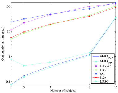
Table 5 shows the clustering results for the various algorithms using different numbers of subjects. The SLRRPCA algorithm almost consistently obtained lower mean clustering errors than the other algorithms for a varying number of subjects. This confirms that our proposed method is very effective and robust against a varying number of subjects with respect to face clustering. We also observed that the clustering performance by SLRRRP outperforms that of SLRRPCA by a very small margin with 10 subjects. However, SLRRRP performs worse than SLRRPCA as well as LRRSC and SSC when the number of subjects is less than 10. However, we also see that increasing the number of clusters of SLRRRP achieved a greater improvement compared with LRR. This phenomenon can be explained as follows. On the one hand, the clustering results of SLRRRP are effected largely by the randomly generated project matrix. On the other hand, what we emphasize is the importance of the determination of low-rank matrix recovery techniques for an alternative low-rank matrix. Moreover, we also compared the computational costs shown in Fig. 5. The computational costs of SLRRPCA and SLRRRP are very similar, and only slightly better than LRSC. LRSC also had relatively low computational time at the expense of degraded performance in the experiments. In fact, SLRRPCA and SLRRRP achieved high efficiency owing to completely avoiding the iterative SVD computation. Both of these run much faster than the other algorithms, e.g., LRR, LRRSC, SSC, and LSA.
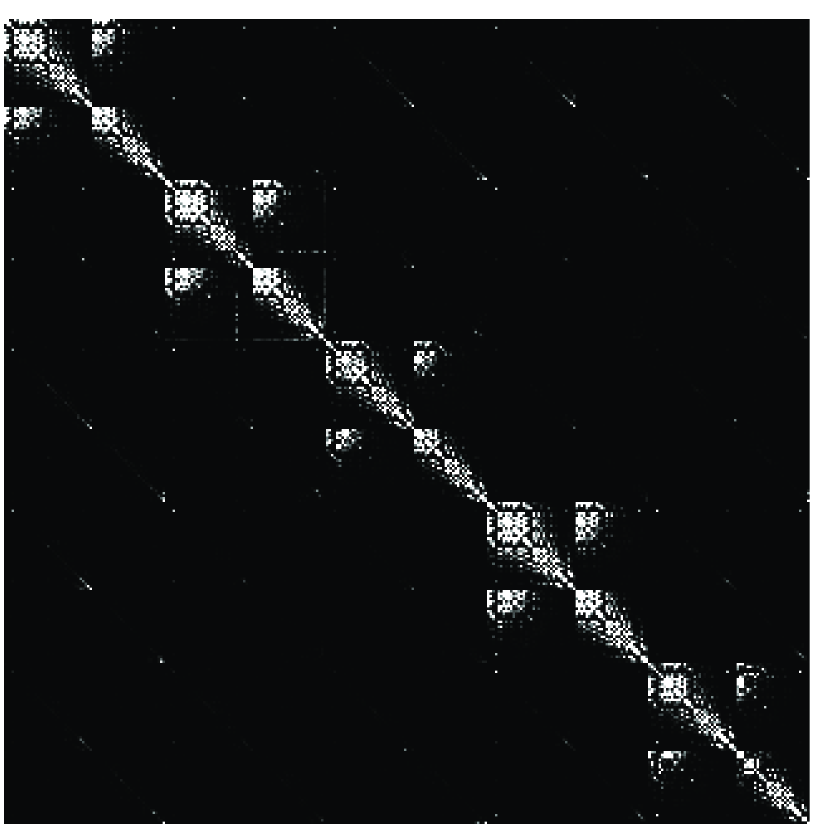
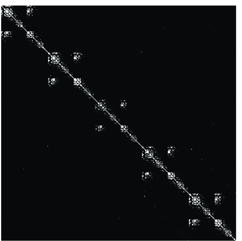
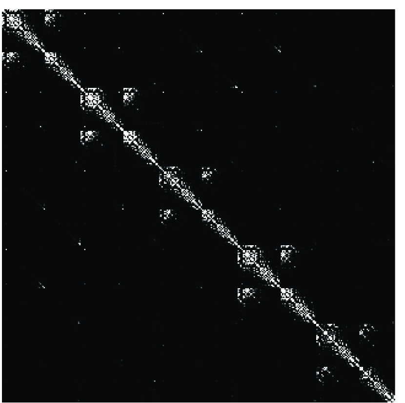
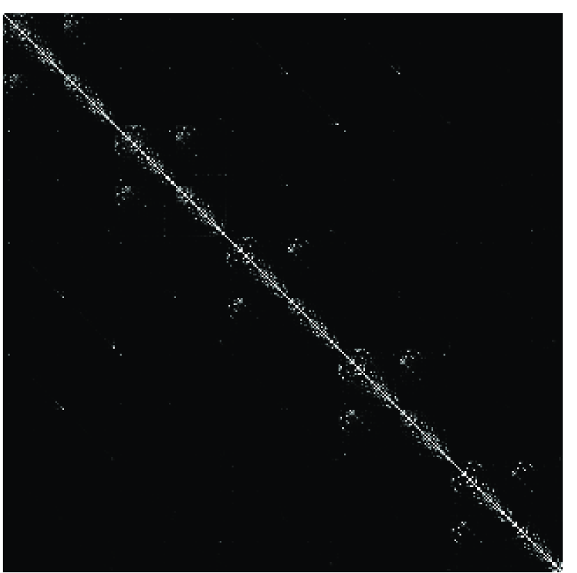
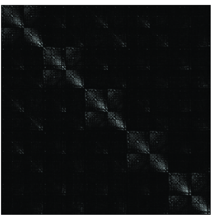
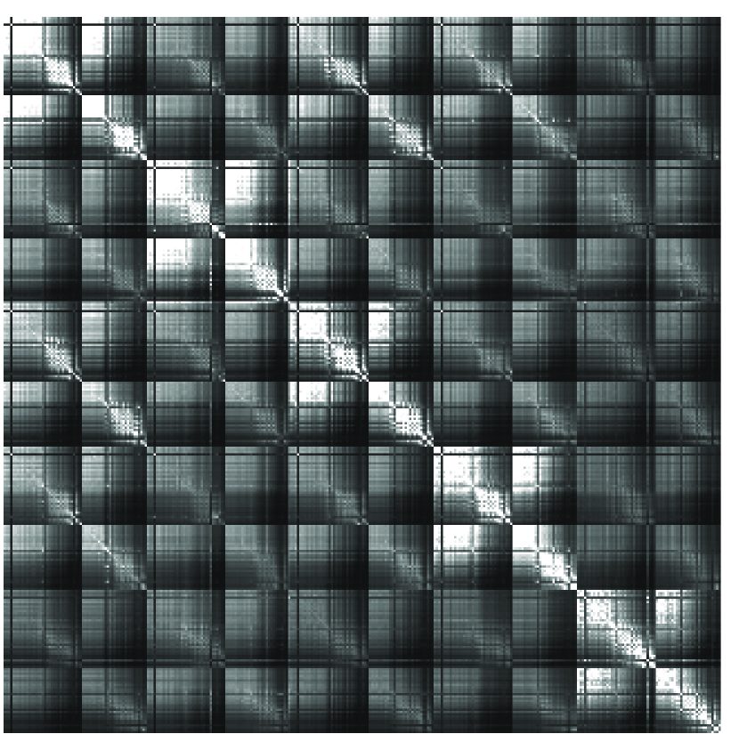
Figure 6 depicts seven representative examples of the affinity graph matrix produced by the different algorithms for the Extended Yale Database B with five subjects. Clearly there are five diagonal blocks in each affinity graph. The smaller the number of non-zero elements lying outside the diagonal blocks is, the more accurate are the clustering results in spectral clustering. It is clear from Fig. 6 that the affinity graph matrix produced by SLRRPCA has a distinct block-diagonal structure as is the case for LRRSC. This shows why SLRRPCA outperforms the other algorithms.
4.3 Experiments on motion segmentation
In this subsection we discuss applying SLRR to the Hopkins 155 database. The task of motion segmentation involves segmenting tracked feature point trajectories of multiple rigidly moving objects into their corresponding motions in a video sequence. Each video sequence is a sole subspace segmentation task. There are 156 video sequences of two or three motions in the Hopkins 155 database. As pointed out in [13], the tracked feature point trajectories for a single motion lie in a low-dimensional subspace. Therefore, the motion segmentation problem is equivalent to the problem of subspace clustering.
For each video sequence, tracked feature point trajectories were extracted automatically and the original data were almost noise-free, i.e., low-rank. Hence, we designed two experiments to evaluate the performance of the proposed SLRR in motion segmentation. First, we used the original tracked feature point trajectories associated with each motion to validate SLRR. Next, we used PCA to project the original data onto a -dimensional subspace, where is the number of motions in each video sequence. Note that both scenarios were implemented in an affine subspace, thereby ensuring that the sum of the feature point trajectory coefficients was .
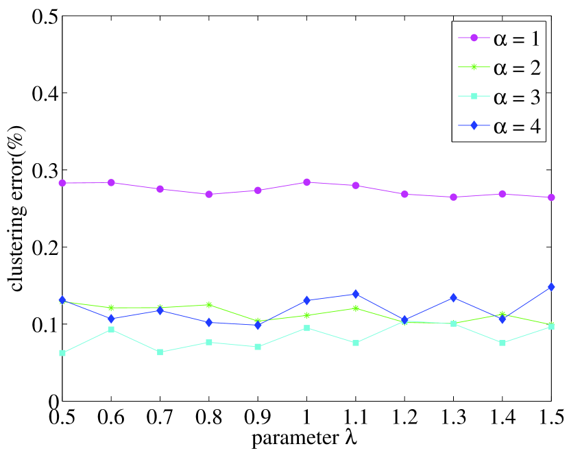
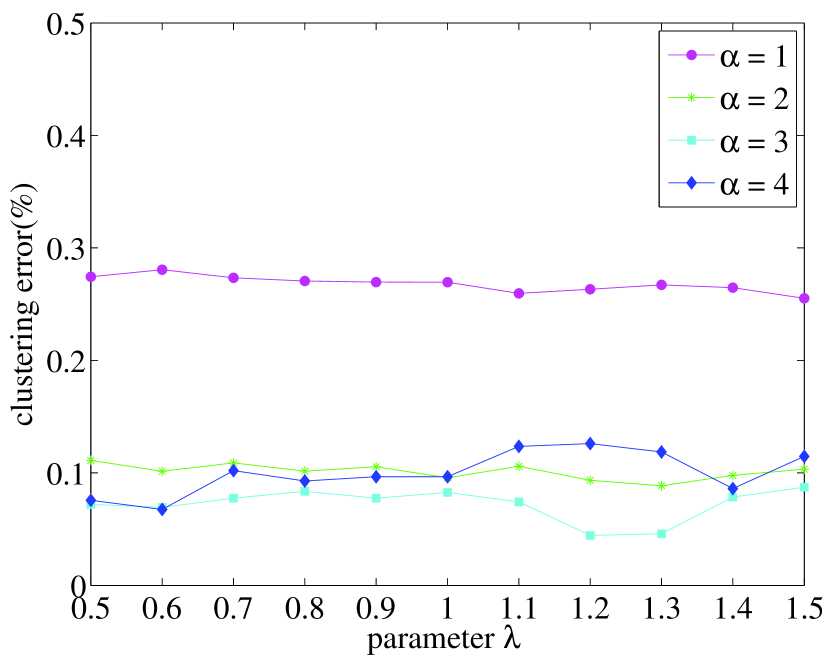
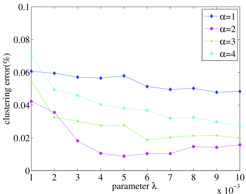
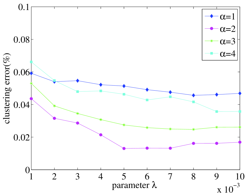
Figures 8 and 8 show the influence of parameters and under two experimental settings of the Hopkins 155 database on the average clustering error of SLRR. It is clear that increasing from 1 to 2 produced higher clustering performance. For example, the clustering error varies from 0.88% to 4.22% while ranges from to with in Fig. 8. If ranges from to , the clustering error appears to change only slightly, varying from 0.88% to 1.04% in Fig. 8. However, SLRR suffers from a decline in clustering performance when continues to increase from 2 to 4 in Fig. 8. We observed a similar influence of parameters and in Fig. 8. This implies that the clustering performance of SLRR on the Hopkins 155 database remains relatively stable for a large range of with .
Tables 6 and 7 show the average clustering errors of the different algorithms on two experimental settings of the Hopkins 155 database. SLRR obtained 0.88% and 1.3% clustering errors for the two experimental settings. In both experimental settings, SLLR significantly outperformed the other algorithms. We used the normalization step of symmetric low-rank representation to improve the clustering performance to further seek an affinity matrix. Under the same parameter settings, we also report the clustering error of SLRR within parentheses without the normalization step in Tables 6 and 7. The normalization step helps improve the clustering results. Compared with LRR, SLRR achieved 0.83% and 0.87% improvement on clustering errors for the two settings, respectively. The improvement comes from the advantages of the compactness of the symmetric low-rank representation. LRR has lower errors than SSC owing to the post-processing of its coefficient matrix. This also confirms the necessity of exploiting the structure of the low-rank representation for an affinity graph matrix. Besides, LRSC still has higher errors than the other algorithms in both experiments.
| Algorithm | Error | Time | |||
|---|---|---|---|---|---|
| mean | median | std. | max. | ||
| SLRR | 0.88 (3) | 0 (0) | 3.63 (9.33) | 38.06 (49.25) | 0.09 (0.09) |
| LRRSC | 1.5 | 0 | 4.36 | 33.33 | 4.71 |
| LRR | 1.71 | 0 | 4.86 | 33.33 | 1.29 |
| SSC | 2.23 | 0 | 7.26 | 47.19 | 1.02 |
| LSA | 11.11 | 6.29 | 13.04 | 51.92 | 3.44 |
| LRSC | 4.73 | 0.59 | 8.8 | 40.55 | 0.14 |
| Algorithm | Error | Time | |||
|---|---|---|---|---|---|
| mean | median | std. | max. | ||
| SLRR | 1.3 (2.42) | 0 (0) | 5.1 (8.14) | 42.16 (49.25) | 0.07 (0.08) |
| LRRSC | 1.56 | 0 | 5.48 | 43.38 | 4.62 |
| LRR | 2.17 | 0 | 6.58 | 43.38 | 0.69 |
| SSC | 2.47 | 0 | 7.5 | 47.19 | 0.93 |
| LSA | 4.7 | 0.6 | 10.2 | 54.51 | 3.35 |
| LRSC | 4.89 | 0.63 | 8.91 | 40.55 | 0.13 |
The computational cost of SLRR is much lower than that of the other algorithms owing to its closed form solution. High clustering performance can also be obtained when the original data are used directly in SLRR. This phenomenon occurs because most sequences are clean, i.e., low-rankness property. However, this does not deny the importance of pursing an alternative low-rank matrix by low-rank matrix recovery techniques. Clean data are not easily obtained because of noise or corruption in real observations.
4.4 Discussion
Our experiments show that the performance of SLRR and LRR differs, with a relative clustering error reduction of more than 10% in some cases. In what follows, we discuss the connection between SLRR and LRR.
First, LRR not only seeks the best low-rank representation of high-dimensional data for matrix recovery, but also recovers the true subspace structures. Contrarily, SLRR focuses only on how to recover the true subspace structures. Generally, differs from in the low-rank representation obtained by LRR, where or depicts the membership between data points and . LRR constructs the affinity for the spectral clustering input using a symmetrization step of the low-rank representation results, i.e., . Evaluating the membership between data points, however, is not good, because LRR attempts to enforce symmetry of the affinity using this trick, whereas SLRR directly models the symmetric low-rank representation, thereby ensuring weight consistency for each pair of data points. The symmetric low-rank representation given by SLRR effectively preserves the subspace structures of high-dimensional data.
Second, SLRR further exploits the intrinsically geometrical structure of the membership of data points preserved in the symmetric low-rank representation. Note that the mechanism for exploiting this has been elaborated in our previous work, i.e., LRRSC [37]. In other words, SLRR makes full use of the angular information of the principal directions of the symmetric low-rank representation so that highly correlated data points of subspaces are clustered together. This is a critical step in calculating the membership between data points. Fig. 6 shows that the block-diagonal structure of the affinity produced by SLRR is more distinct and compact than that obtained by LRR. The experimental results demonstrate that this significantly improves subspace clustering performance.
Finally, SLRR provides a more flexible model of the low-rank representation. SLRR integrates the collaborative representation combined with low-rank matrix recovery techniques into a low-rank representation with respect to various types of noise, e.g., Gaussian noise and arbitrary sparse noise. Additionally, it avoids iterative SVD operations while learning a symmetric low-rank representation. However, we need to emphasize that SLRR does not pursue the lowest-rank representation of data for evaluating the membership between data points. Strictly speaking, it does not make sense to pursue only the lowest-rank representation of data. Let us consider the LRR model again. The corresponding optimal solution can be obtained for an arbitrary value of parameter in problem (3). Obviously, we cannot determine which low-rank matrix of the optimal solution is desirable without prior knowledge of the data set. Hence, it is reasonable that SLRR tries to obtain a symmetric low-rank representation of the data. This also explains why we use the constraint, , to guarantee the low-rank property of the symmetric representation of the data in problem (5) or (8). In fact, in our experiments, we have also discussed some of the detail involved in estimating the rank of a data matrix of images of various examples, for example, images of an individual s face and handwritten images of a digit.
5 Conclusions
In this paper we presented a method called SLRR, which considers collaborative representation combined with low-rank matrix recovery techniques to create a low-rank representation for robust subspace clustering. Unlike time-consuming SVD operations in many existing low-rank representation based algorithms, SLRR involves learning a symmetric low-rank representation in a closed form solution by solving the symmetric low-rank optimization problem, which greatly reduces computational cost in practical applications. Experimental results on benchmark databases demonstrated that SLRR is efficient and effective for subspace clustering compared with several state-of-the-art subspace clustering algorithms.
SLRR is a simple and effective method, which is considered an improvement over our previously proposed LRRSC [37]. However, several problems remain to be solved. In the implementation of SLRR, it is important how to introduce low-rank matrix recovery algorithms, because a proper alternative low-rank matrix may significantly improve the subspace clustering performance. In addition, the determination of the parameter for pursing an alternative low-rank matrix by low-rank matrix recovery or feature extraction is also an intractable problem. Moreover, it is difficult to estimate a suitable value of without prior knowledge. In future work, we will investigate these problems for practical applications.
Acknowledgements
The authors would like to thank the anonymous reviewers for their valuable comments and suggestions. This research was supported by the National Basic Research Program of China (973 Program) under Grant 2011CB302201 and the National Science Foundation of China under Grant 61303015.
References
- Eldar and Mishali [2009] Y. C. Eldar, M. Mishali, Robust recovery of signals from a structured union of subspaces, IEEE Trans. Inf. Theor. 55 (2009) 5302–5316.
- Liu et al. [2013] G. Liu, Z. Lin, S. Yan, J. Sun, Y. Yu, Y. Ma, Robust recovery of subspace structures by low-rank representation, IEEE Trans. Pattern Anal. and Mach. Intell. 35 (2013) 171–184.
- Liu et al. [2010] G. Liu, Z. Lin, Y. Yu, Robust subspace segmentation by low-rank representation, In ICML (2010).
- Elhamifar and Vidal [2013] E. Elhamifar, R. Vidal, Sparse subspace clustering algorithm, theory, and applications, IEEE Trans. Pattern Anal. and Mach. Intell. 35 (2013) 2765–2781.
- Rao et al. [2008] S. Rao, R. Tron, R. Vidala, Y. Ma, Motion segmentation via robust subspace separation in the presence of outlying, incomplete, or corrupted trajectories, In CVPR (2008).
- Lauer and Schnrr [2009] F. Lauer, C. Schnrr, Spectral clustering of linear subspaces for motion segmentation, in IEEE International Conference on Computer Vision (2009) 678–685.
- Rao et al. [2010] S. Rao, R. Tron, R. Vidal, Y. Ma, Motion segmentation in the presence of outlying, incomplete, or corrupted trajectories, IEEE Trans. Pattern Anal. and Mach. Intell. 32 (2010) 1832–1845.
- Aldroubi and Sekmen [2012] A. Aldroubi, A. Sekmen, Nearness to local subspace algorithm for subspace and motion segmentation, IEEE Signal Processing Letters 19 (2012) 704–707.
- Vidala and Favarob [2013] R. Vidala, P. Favarob, Low rank subspace clustering (LRSC), Pattern Recognition Letters (2013).
- Vidal [2010] R. Vidal, A tutorial on subspace clustering, IEEE Signal Processing Magazine 28 (2010) 52–68.
- Sim et al. [2013] K. Sim, V. Gopalkrishnan, A. Zimek, G. Cong, A survey on enhanced subspace clustering, Data mining and knowledge discovery 26 (2013) 332–397.
- McWilliams and Montana [2014] B. McWilliams, G. Montana, Subspace clustering of high-dimensional data: a predictive approach, Data Mining and Knowledge Discovery 28 (2014) 736–772.
- Boult and Brown [1991] T. Boult, L. Brown, Factorization-based segmentation of motions, in IEEE Workshop on Proceedings of the Visual Motion (1991) 179–186.
- Basri and Jacobs [2003] R. Basri, D. W. Jacobs, Lambertian reflectance and linear subspaces, IEEE Trans. Pattern Anal. and Mach. Intell. 25 (2003) 218–233.
- Dyer et al. [2013] E. Dyer, A. Sankaranarayanan, R. Baraniuk, Greedy feature selection for subspace clustering, The Journal of Machine Learning Research 14 (2013) 2487–2517.
- Vidal et al. [2005] R. Vidal, Y. Ma, S. Sastry, Generalized principal component analysis (GPCA), IEEE Trans. Pattern Anal. and Mach. Intell. 27 (2005) 1945–1959.
- Fischler and Bolles [1981] M. Fischler, R. Bolles, Random sample consensus: a paradigm for model fitting with applications to image analysis and automated cartography, Communications of the ACM 24 (1981) 381–395.
- Ho et al. [2003] J. Ho, M. Y. J. Lim, K. Lee, D. Kriegman, Clustering appearances of objects under varying illumination conditions, In CVPR (2003).
- Ni et al. [2010] Y. Ni, J. Sun, S. Y. X.J. Yuan, L. Chong, Robust low-rank subspace segmentation with semidefinite guarantees, Proceedings of the IEEE International Conference on Data Mining Workshops (ICDMW) (2010) 1179–1188.
- L.Zhuang et al. [2012] L.Zhuang, H. Gao, Z. Lin, Y. Ma, X. Zhang, N. Yu, Non-negative low rank and sparse graph for semi-supervised learning, In CVPR (2012).
- Peng et al. [2012] X. Peng, L. Zhang, Z. Yi, Constructing the l2-graph for subspace learning and subspace clustering, arXiv preprint arXiv:1209.0841 (2012).
- Costeira and Kanade [1998] J. P. Costeira, T. Kanade, A multibody factorization method for independently moving objects, Int. J. Comput. Vision 29 (1998) 159–179.
- Wei and Lin [2011] S. Wei, Z. Lin, Analysis and improvement of low rank representation for subspace segmentation, arXiv:1107.1561 (2011).
- Liu et al. [2012] R. Liu, Z. Lin, F. Torre, Z. Su, Fixed-rank representation for unsupervised visual learning, In CVPR (2012).
- Liu et al. [2013] Y. Liu, L. Jiao, F. Shang, An efficient matrix factorization based low-rank representation for subspace clustering, Pattern Recognition 46 (2013) 284–292.
- Zhang et al. [2014] H. Zhang, Z. Yi, X. Peng, flrr: fast low-rank representation using frobenius-norm, Electronics Letters 50 (2014) 936–938.
- Luxburg [2007] U. V. Luxburg, A tutorial on spectral clustering, Statistics and computing 17 (2007) 395–416.
- Shi et al. [2000] J. Shi, J. Malik, S.Sastry, Normalized cuts and image segmentation, IEEE Trans. Pattern Anal. and Mach. Intell. 22 (2000) 888–905.
- Tibshiran [1996] R. Tibshiran, Regression shrinkage and selection via the lasso, Journal of the Royal Statistical Society Series B 58 (1996) 267–288.
- Donoho [2006] D. Donoho, For most large underdetermined systems of linear equations the minimal -norm solution is also the sparsest solution, Comm. Pure and Applied Math. 59 (2006) 797–829.
- Cands et al. [2008] E. J. Cands, M. B. Wakin, S. P. Boyd, Enhancing sparsity by reweighted minimization, Journal of Fourier Analysis and Applications 14 (2008) 877–905.
- Nasihatkon and Hartley [2011] B. Nasihatkon, R. Hartley, Graph connectivity in sparse subspace clustering, in CVPR (2011) 2137–2144.
- Wang and Xu [2013] Y. Wang, H. Xu, Noisy sparse subspace clustering, arXiv preprint arXiv:1309.1233 (2013).
- Bao et al. [2012] B. Bao, G. Liu, C. Xu, S. Yan, Inductive robust principal component analysis, IEEE Trans. Image Processing 21 (2012) 3794–3800.
- Z. Lin and Ma [2010] M. C. Z. Lin, Y. Ma, The augmented lagrange multiplier method for exact recovery of corrupted low-rank matrices, arXiv preprint arXiv:1009.5055 (2010).
- Lin et al. [2011] Z. Lin, R. Liu, Z. Su, Linearized alternating direction method with adaptive penalty for low-rank representation, In NIPS (2011).
- Chen and Yi [2014] J. Chen, Z. Yi, Subspace clustering by exploiting a low-rank representation with a symmetric constraint, arXiv preprint arXiv:1403.2330 (2014).
- Zhang et al. [2011] L. Zhang, M. Yang, X. Feng, Sparse representation or collaborative representation: Which helps face recognition?, In ICCV (2011) 471–478.
- Lu et al. [2012] C. Lu, H. Min, Z. Zhao, L. Zhu, D. Huang, S. Yan, Robust and efficient subspace segmentation via least squares regression, In ICCV (2012) 347–360.
- Wang et al. [2011] S. Wang, X. Yuan, T. Yao, S. Yan, J. Shen, Efficient subspace segmentation via quadratic programming, In AAAI (2011).
- Jolliffe [2002] I. Jolliffe, Principal Component Analysis, Springer New York, 2002.
- Wright et al. [2009] J. Wright, A. Ganesh, S. Rao, Y. Peng, Y. Ma, Robust principal component analysis: Exact recovery of corrupted low-rank matrices by convex optimization, In NIPS (2009) 2080–2088.
- Cands et al. [2011] E. J. Cands, X. Li, Y. Ma, J. Wright, Robust principal component analysis, Journal of the ACM (JACM) 58 (2011).
- Kaski [1998] S. Kaski, Dimensionality reduction by random mapping: Fast similarity computation for clustering, IEEE International Joint Conf. Neural Networks Proceedings (1998) 413–418.
- Bingham and Mannila [2001] E. Bingham, H. Mannila, Random projection in dimensionality reduction: applications to image and text data, Proc. ACM SIGKDD international Conf. Knowledge discovery and data mining (2001) 245–250.
- Lee et al. [2005] K. Lee, J. Ho, D. Kriegman, Acquiring linear subspaces for face recognition under variable lighting, IEEE Trans. Pattern Anal. and Mach. Intell. 27 (2005) 684–698.
- Georghiades et al. [2011] A. Georghiades, P. Belhumeur, D. Kriegman, From few to many: Illumination cone models for face recognition under variable lighting and pose, IEEE Trans. Pattern Anal. and Mach. Intell. 23 (2011) 643–660.
- Tron and Vidal [2007] R. Tron, R. Vidal, A benchmark for the comparison of 3-d motion segmentation algorithms, In CVPR (2007).
- Yan and Pollefeys [2006] J. Yan, M. Pollefeys, A general framework for motion segmentation: Independent, articulated, rigid, non-rigid, degenerate and non-degenerate, In European Conf. on Computer Vision (2006) 94–106.