Dynamic Model Averaging in Large Model Spaces Using Dynamic Occam’s Window

Abstract

Bayesian model averaging has become a widely used approach to accounting for uncertainty about the structural form of the model generating the data. When data arrive sequentially and the generating model can change over time, Dynamic Model Averaging (DMA) extends model averaging to deal with this situation. Often in macroeconomics, however, many candidate explanatory variables are available and the number of possible models becomes too large for DMA to be applied in its original form. We propose a new method for this situation which allows us to perform DMA without considering the whole model space, but using a subset of models and dynamically optimizing the choice of models at each point in time. This yields a dynamic form of Occam’s window. We evaluate the method in the context of the problem of nowcasting GDP in the Euro area. We find that its forecasting performance compares well that of other methods.

Keywords: Bayesian model averaging; Model uncertainty; Nowcasting; Occam’s window.

1 Introduction

In macroeconomic forecasting, there are often many available candidate predictor variables, and uncertainty about precisely which ones should be included in the forecasting model. Accounting for this uncertainty is important, and Bayesian model averaging (BMA) (Leamer, 1978; Raftery, 1988; Madigan and Raftery, 1994; Raftery, 1995; Raftery et al., 1997; Hoeting et al., 1999) has emerged as an established way of doing so, thanks in large part to methodological developments to which Eduardo Ley has contributed (Fernández and Steel, 2001; Fernández et al., 2001; Ley and Steel, 2007, 2009). For other developments of BMA in macroeconomics, see Brock and Durlauf (2001), Brock et al. (2003), Sala-i-Martin et al. (2004), Durlauf et al (2006, 2008), Eicher et al. (2010) and Varian (2014); see Steel (2011) for a survey.

Model averaging has been found useful in economics for several reasons. These include the possibility of using more parsimonious models, which tend to yield more stable estimates, because fewer degrees of freedom are used in individual models. Also, BMA yields the posterior inclusion probability for each variable, making the results easy to interpret. Further, when compared to large scale models with the same variables, BMA provides automatic shrinkage through the parsimony of the individual models. It can be used to account for uncertainty about the best way to measure a concept, such as different measures of slack in a Phillips curve. It can also be used to account for uncertainty about model structure beyond variable selection (e.g. linear versus nonlinear, univariate versus multivariate, fixed versus time-varying parameters).

BMA is a static method, and as such cannot deal with the situation where data arise sequentially (as is generally the case in macroeconomics), and the form of the generating model can change over time. To deal with this, Dynamic Model Averaging (DMA) was proposed by Raftery et al. (2010). This allows both the model form and the model parameters to change over time and tracks both recursively.

DMA requires the evaluation of each model at each time point. Often in macroeconomics, however, many candidate predictor variables are available. Typically, the number of candidate regression models is equal or close to $2^{J}$, where $J$ is the number of candidate predictor variables. This grows rapidly with $J$, and so the number of possible models becomes too large for it to be computationally feasible for DMA to be applied in its original form.

We propose a way of implementing DMA in large model spaces, called Dynamic Occam’s Window (DOW). This allows us to perform DMA without considering the whole model space, but using a subset of models and dynamically optimizing the choice of models at each point in time. It is particularly adapted to macroeconomic studies and allowing the inclusion of big information sets. Our proposal allows us to run DMA without an exhaustive exploration of the space of models. We describe an application to the difficult problem of nowcasting GDP in the euro area.

The paper is organized as follows. Section 2 briefly reviews Bayesian and Dynamic Model Averaging and Model Selection. In Section 3 we describe the Dynamic Occam’s Window method. In Section 4 we describe an economic application, the nowcasting of the euro area GDP, and show in Section 5 that the results of our technique compare well with others in the existing literature in terms of forecasting performance and computational efficiency. Section 6 gives the results of several sensitivity analyses, and the final section concludes.

2 Forecasting with Dynamic Model Averaging

Here we outline the main concept of Dynamic Model Averaging (DMA), introduced by Raftery et al. (2010). Assume a population, $M$, of $K$ candidate regression models, $M=\{m_{1},..,m_{K}\}$, where model $m_{k}$ takes the form:

$$y_{t}=x_{t}^{\left(k\right)}\beta_{t}^{\left(k\right)}+\varepsilon_{t}^{\left(k\right)}\\ ,\qquad$$

where $\varepsilon_{t}^{\left(k\right)}\sim N\left(0,\sigma_{t}^{2\left(k\right)}\right)$ .

Each explanatory set $x_{t}^{\left(k\right)}$ contains a subset of the potential explanatory variables $x_{t}$. It can be seen immediately that this implies a large number of models: if $J$ is the number of explanatory variables in $x_{t}$ there are $K=$ $2^{J}$ possible regression models involving every possible combination of the $J$ explanatory variables.

DMA averages across models using a recursive updating scheme. At each time two sets of weights are calculated, $w_{t|t-1,k}$ and $w_{t|t,k}$. The first, $w_{t|t-1,k}$, is the key quantity. It is the weight of model $k$ in forecasting $y_{t}$ given data available at time $t-1$. The second weight, $w_{t|t,k}$, is the update of $w_{t|t-1,k}$ using data available at time $t$. DMA produces forecasts which average over all $K$ models using $w_{t|t-1,k}$ as weights. Note that DMA is dynamic since these weights can vary over time.

Dynamic Model Selection (DMS) is similar but it involves selecting the model with the highest value for $w_{t|t-1,k}$ and using it for forecasting $y_{t}$. DMS allows for model switching: at each point in time it is possible that a different model is chosen for forecasting.

Raftery et al. (2010) derive for DMA the following updating equation:

$$w_{t|t,k}=\frac{w_{t|t-1,k}L_{k}\left(y_{t}|y_{1:t-1}\right)}{\sum_{\ell=1}^{K}w_{t|t-1,\ell}L_{\ell}\left(y_{t}|y_{1:t-1}\right)},$$ (1)

where $L_{k}\left(y_{t}|y_{1:t-1}\right)$ is the predictive likelihood, or the predictive density of $y_{t}$ for model $m_{k}$ evaluated at the realized value of $y_{t}$. The algorithm then produces the weights to be used in the following period by using a forgetting factor, $\alpha$:

$$w_{t+1|t,k}=\frac{w_{t|t,k}^{\alpha}}{\sum_{\ell=1}^{K}w_{t|t,\ell}^{\alpha}}.$$ (2)

The forgetting factor, $\alpha$, is specified by the user. Here we use $\alpha=0.99$, following Raftery et al. (2010).

Thus, starting with $w_{0|0,k}$ (for which we use the noninformative choice of $w_{0|0,k}=\frac{1}{K}$ for $k=1,..,K$) we can recursively calculate the key elements of DMA: $w_{t|t,k}$ and $w_{t|t-1,k}$ for $k=1,..,K$.

3 Dynamic Occam’s Window

When many potential regressors are considered, the number of models is too high to be tractable. However, typically the great majority of models contribute little to the forecast, as their weights are close to zero. These include for example highly misspecified models, which are kept despite their poor performance only to calculate equation (2).

We propose a heuristic aiming at eliminating most of these low probability models from the computation, while being able to “resurrect” them when needed. This is based on the Occam’s Window method of Madigan and Raftery (1994), in which model averaging is based only on models whose posterior model probability is greater than some multiple $C$ of the highest model probability. (Madigan and Raftery (1994) used $C=1/20$, while subsequent implementations have used lower values.)

We now extend Occam’s Window to the dynamic context. Our Dynamic Occam’s Window (DOW) method is based on two implicit assumptions:

1. We dispose at the initial time of a valid population of models

2. Models do not change too fast over time: the relevant models at each time are close enough (in a “neighbourhood” opportunely defined) to those of the preceding time.

We believe these assumptions are reasonable in typical problems of macroeconomic analysis. If verified, they allow the exploration of the space of models in a parsimonious and efficient way.

3.1 Forecast, Expand, Assess, Reduce: the FEAR algorithm

We propose to implement Occam’s window on currently used models and keep for future use only those that perform sufficiently well relative to the best performer. Call the current set of models $M_{0}(t)$, and renormalize their current weights, $w_{t|t,k}$, so that they sum to 1 over the current set of models, i.e. so that $\sum_{k:m_{k}\in M_{0}(t)}w_{t|t,k}=1$. After choosing a threshold $C\in(0,1]$, we keep for future use the models $m_{k}\in M_{0}(t)$ that fall in Occam’s window, namely

$$m_{k}:m_{k}\in M_{0}(t),w_{t|t,k}\geq C*\max_{\ell:m_{\ell}\in M_{0}(t)}w_{t|t,\ell}.$$ (3)

The FEAR algorithm iterates four steps: Forecasting, Expanding the set of models, Assessing them, and Reducing the model set via Occam’s window.

Initialization

1. Divide the sample $1,\ldots,T$ into a training sample $1,\ldots,T_{r}$ and a forecasting/evaluation sample $T_{r+1},\ldots,T$

2. Start with an initial population of models $M_{0}(T_{r})$ and an initial set of weights $w_{T_{r}|T_{r},k}$.

For $t=(T_{r}+1),\ldots,T$:

1. (Forecast) Use the models in $M_{0}(t-1)$ and the weights $w_{t|t-1,k}$ to perform model averaging as in Raftery et al. (2010), obtaining the forecast distribution $p(y_{t}|y_{1:t-1},M_{0}(t-1))$.

2. (Expand) Expand $M_{0}(t-1)$ into a larger population $M_{1}(t)$ including all $m_{k}\in M_{0}(t-1)$ and all their neighbouring models (all models derived from any model $m\in M_{0}(t-1)$ by adding or subtracting a regressor).

3. (Assess) Upon observing $y_{t}$ compute for all $m_{k}\in M_{1}(t)$ the weights $w_{t|t,k}$, normalized to sum to 1 over $M_{1}(t)$.

4. (Reduce) Define the final population of models for time $t$, $M_{0}(t)$, as those in $M_{1}(t)$ that are in Occam’s Window, namely $M_{0}(t)=\{m_{k}\in M_{1}(t):w_{t|t,k}\geq C*\max_{\ell:m_{\ell}\in M_{1}(t)}w_{t|t,\ell}\}$.

End for

3.2 Computational issues

This section explains why Dynamic Occam’s Window allows the exploration of large models spaces that would not be possible otherwise.

We define, rather imprecisely but as a rough reference, a Notional Unit of Computation (NUC) as a basic operation of estimation. Since we are concentrating on computability, we consider broadly equivalent (one NUC) one OLS estimation, one period estimation of a Kalman filter and in general each operation involving at least a matrix inversion. On this loosely defined but quite general metric we compare the DOW method with a DMA exhaustively exploring the space of models. Let $J$ be the number of candidate explanatory variables, $T$ be the number of time points for which we have data, and $N$ be the number of models in Occam’s window (a subset of the $K$ possible regression models).

DMA with all models has approximate computational cost

$${\rm NUC}_{\rm DMA}=2^{J}*T,$$ (4)

because all the potential models need to be estimated once per period.

The DOW method reduces the number of models to be evaluated but changes the population dynamically. It is therefore necessary to re-estimate each model from the beginning each time. Its computational cost is thus approximately that of estimating about

$${\rm NUC}_{\rm DOW}=\frac{(T+1)*T}{2}*N$$ (5)

different models. The role of the number of models $N$ is explored in Section 6.

The DOW method allows gains in speed when ${\rm NUC}_{\rm DOW}<{\rm NUC}_{\rm DMA}$, or

$$N<2*\frac{2^{J}}{(nT+1)}.$$ (6)

To illustrate, consider the case where $T$ = 45, $J$ = 25, and $N$ varies. Then for $N=1000$

$$\frac{{\rm NUC}_{\rm DOW}}{{\rm NUC}_{\rm DMA}}=\frac{10.350.000}{1.509.949.440}=0.68\%.$$ (7)

Thus the DOW method is about 150 times faster.

Figure 1: Computing Time: The number of NUC (vertical axis) plotted against the data length and the number of regressors. The blue area refers to the DOW method, the red area to DMA.

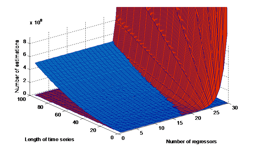
Figure 1 shows the relationships (4) and (5). The computational complexity of the DOW method grows quadratically with the length of the available series $T$, while that of DMA grows only linearly in $T$ but increases exponentially in the number of regressors $J$. Above 15-20 regressors the DOW method is always more efficient computationally. This is particularly true when the time series are relatively short, since longer series imply a higher number of estimations for each model in the case of Occam’s window.

4 An Economic Application: Forecasting GDP in the Euro Area in the Great Recession

4.1 The Forecasting Application

Short term forecasting and nowcasting economic conditions is important for policy makers, investors and economic agents in general. Given the lags in compiling and releasing key macroeconomic variables, it is not surprising that particular attention is paid to nowcasting, an activity of importance because it allows economic decisions to be made and policy actions to be taken with a more precise idea of the current situation.

We apply the DOW method to nowcasting GDP in the euro area. This problem is particularly difficult because there are many candidate explanatory variables (large $J$) but most of them cover a short time span (small $T$). We use quarterly (or converted to quarterly) series available from 1997, and we describe our source data in Table 1. Abstracting from minor differences in publication dates, there are two main GDP nowcasts that a forecaster may perform, depending on whether or not the preceding quarter figure for GDP is available. For simplicity of exposition, we focus on the case when the past quarter is already available. Our nowcasts will be based on an information set comprising past GDP and current indicators.

Table 1: Variables Used in the Euro Area GDP Forecasting Area Application

CODE	VARIABLE	TRANSFORMATION	DATA SOURCE
hicp	Euro area - HICP, Eurostat	Annual growth rate	Eurostat
hicpx	Euro area - HICP excl. unprocessed food an energy, Eurostat	Annual growth rate	Eurostat
ppi	Euro area - Producer Price Index, domestic sales, Total Industry (excluding construction) - Neither seasonally nor working day adjusted	Annual growth rate	Eurostat
unemp	Euro area - Standardised unemployment, Rate, Total (all ages), Total (male & female), percentage of civilian workforce	Level	Eurostat
ip	Euro area - Industrial Production Index, Total Industry (excluding construction) - Working day adjusted, not seasonally adjusted	Annual growth rate	Eurostat
l1 to l5	Euro area - Gross domestic product at market price, Chain linked, ECU/euro, Working day and seasonally adjusted	Annual growth rate	Eurostat
spfgdp2	Survey Professional Forecasters; Forecast topic: Real GDP; Point forecast	Annual growth rate	ECB
spfgdp2_var	Survey Professional Forecasters; Forecast topic: Real GDP; Variance of Point forecast	Variance	ECB
pmi_e	PMI employment	Level	Markit
pmi_ord	PMI new orders	Level	Markit
pmi_y	PMI output	Level	Markit
x_oil	Brent crude oil 1-month Forward - fob (free on board) per barrel - Historical close, average of observations through period - Euro	Annual growth rate	ECB
x_rawxene	Euro area , ECB Commodity Price index Euro denominated, import weighted, Total non-energy commodity	Annual growth rate	ECB
x_neer	Nominal effective exch. Rate	Annual growth rate	ECB
xusd	Exchange Rates; Currency: US dollar; Currency denominator: Euro; Exchange rate type: Spot	Annual growth rate	ECB
i_short	Euro area - Money Market - Euribor 1-year - Historical close, average of observations through period - Euro	Level	Reuters
i_long	Euro area - Benchmark bond - Euro area 10-year Government Benchmark bond yield - Yield - Euro	Level	ECB
m3	Euro Area - Monetary aggregate M3, All currencies combined - Working day and seasonally adjusted	Annual growth rate	ECB
spread	Government bond, nominal yield, all issuers whose rating is triple A (less) Government bond, yield nominal, all issuers all ratings included	Level	ECB
stress	Composite Indicator of Systemic Stress; Euro area ; Systemic Stress Composite Indicator	Level	ECB
risk_eb	Euro area , Financial market liquidity indicator: Foreign currency, equity and bond markets	Level	ECB
risk_tot	Euro area , Financial market liquidity indicator: Composite indicator	Level	ECB
risk_glob	Euro area , Financial market liquidity indicator: Global risk aversion indicator	Level	ECB
risk_mon	Euro area , Financial market liquidity indicator: Money market	Level	ECB
stox	Dow Jones Eurostoxx 50 Index - Historical close, average of observations through period	Annual growth rate	Reuters
domcred	Euro area , Loans [A20] and securities [AT1], Total maturity, All currencies combined - Working day and seasonally adjusted	Annual growth rate	ECB

The need to use timely indicators largely dictates the choice of potential regressors, but most sectors and economic concepts are well covered. Our indicators include domestic prices (HICP, HICP excluding food an energy and producer prices), cycle indicators (unemployment rate, industrial production, lags of GDP), expectations (mean and dispersion of 2 years-ahead SFP forecasts for GDP, PMI for employment, orders and output), prices of commodities (oil prices, non-energy commodity prices), exchange rates (nominal effective exchange rate, EUR/USD exchange rate), monetary policy variables (short and long interest rates, M3), financial variables (spread between interest rate on bonds of AAA states and average interest rate on bonds, Dow Jones Eurostoxx index, domestic credit). Given the relevance of uncertainty in the macroeconomic developments included in our sample, we also include potential macroeconomic risk indicators (Composite Indicator of Systemic Stress, Risk Dashboard data on banking, total, global and monetary factors).

All variables are on the year-on-year growth rate scale, with the exception of interest rates and indicators. The target variable in our forecasting exercises is the year-on-year GDP growth rate. As a result, at least four lags of the independent variable must be included as potential regressors; we use five to account for potential autocorrelation in the residuals. This may be overcautious, but unnecessary lags will be selected away in the model averaging. The possibility of adding regressors but discarding them adaptively if they are unnecessary is one of the advantages of our methodology.

In order to concentrate on the effects of the proposed DOW method, we simplify the method of Raftery et al. (2010) slightly, and estimate each model recursively but with fixed parameters. We choose this setup because (Koop and Korobilis, 2012) have shown that DMA is a good substitute for time varying parameters, and we want to concentrate on the advantages of the DOW method alone in accounting for model changes. DMA is performed as in Raftery et al. (2010), using a discount factor set at $\alpha=0.99$.

4.2 Forecasting Performance

Figure 2 shows that the DOW method had a satisfactory nowcasting performance overall, even in the presence of turning points. The accuracy of the method, as expected, increased with the available data. The 95 per cent error bands take into account the within and between model uncertainty.

Figure 2: Euro Area GDP: Nowcasting and uncertainty bands using the DOW method

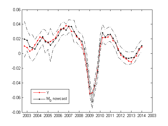
The difficult episode of the recession in 2008-2009 is well captured by DMA. The forecast slightly underpredicts in the trough, but it immediately recovers and becomes quite accurate in the aftermath of the crisis.

Table 2 compares the forecasting performance in a pseudo-real time exercise. Practically all the indicators we use are seldom or never revised, the main difference with a real time forecasting exercise being the fact that we use the latest available vintage for GDP. The evaluation sample ranges from 2003q1 until 2014q1.

Table 2: Forecasting Performance of Different Forecasting Methods

	RW	AR2	DMA-R	DMA-E	DMS-R	DMA-E
RMSE	0.0101	0.0088	0.0043	0.0043	0.0048	0.0048
MAE	0.0067	0.0059	0.0033	0.0033	0.0035	0.0035
MAX	0.0332	0.0376	0.0125	0.0126	0.0139	0.0139

Note: Methods: RW = Random walk model; AR2 = second-order autoregressive model; DMA-R = reduced DMA method; DMA-E = expanded DMA method; DMS-R = reduced DMS method; DMS-E = expanded DMS method.
Metrics: RMSE = root mean squared error; MAE = mean absolute error; MAX = maximum absolute error. The best method by each metric is shown in bold font.

The DMA-R forecast is based on the smaller population of models $M_{0}$ and compares favourably with simple benchmarks. It largely beats both the simple random walk and a standard $AR(2)$. We recall that the forecast DMA-R is based on past GDP and recent information on the indicator variables.

Forecasts computed using the extended population of models $M_{1}$ are reported as DMA-E. The results are very close to those of DMA-R. When there are differences in the assessment, these are not sizeable and completely disappear if a sufficient size for population $M_{0}$ is allowed. Intuitively, the population $M_{1}$ has the advantage of always including all regressors in its models and as a consequence it should react more quickly to model changes. On the other hand its forecast is slightly more noisy due to the presence of additional models. The two effects basically cancel out. DMA-R uses many fewer models than DMA-E and so may be preferred to DMA-E on the grounds of simplicity, ease of interpretation and computational efficiency.

Each DMA method beats the corresponding forecast computed with DMS, although by a small margin, corroborating the common finding that model averaging can beat even the best model in the pool.

We also implemented DMA using models with time varying parameters. In our case, this tended to overreact to the crisis, showing poorer performance. We interpret this result as hinting that changes in models during the crisis were not due to strong nonlinearities in the model but to the appearance of new regressors.

Following Koop and Korobilis (2012), we tried additional benchmarks. These included a single time-varying parameter model including all regressors, and a single Bayesian ordinary least squares model with all regressors. However, these models either could not be estimated or performed very poorly as their estimated paramaters were very unstable.

4.3 Further results

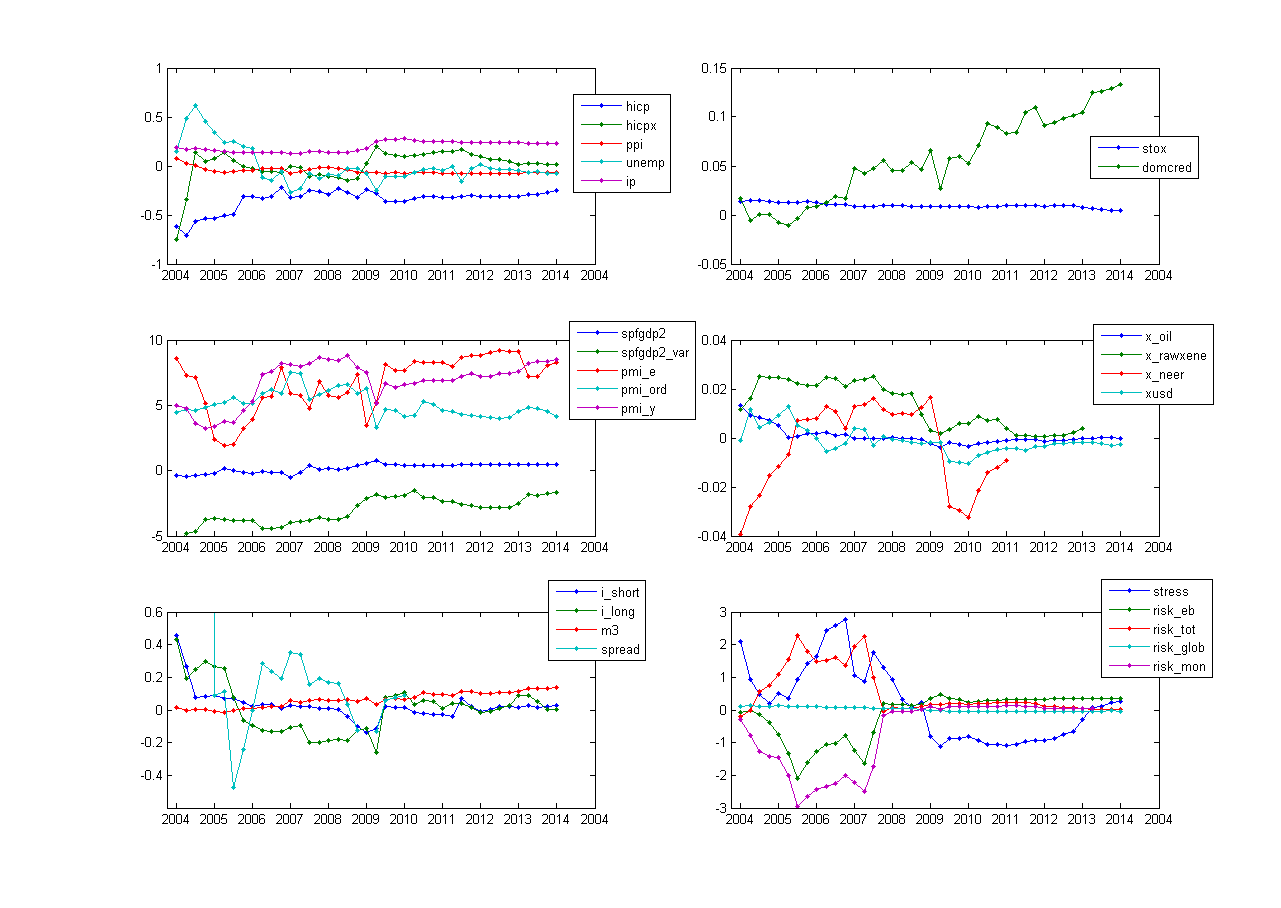
An important value added (beyond the good forecasting performance) of using model averaging concerns the inclusion probabilities of each regressor and their evolution. DMA identifies the importance of single variables and how this varies over time, which helps interpretation. The inclusion probability of a variable at a given time point is calculated by summing up the weights of the models that use that variable as a regressor. Thus they vary between 0 and 1 and give a measure of the importance of that regressor. Their evolution in time is summarized in Figures 3 and 4.

Figure 3: Inclusion probabilities of variables over time: (black) above 10%, (red) above 50%

Figure 4: Inclusion probabilities of single variables over time

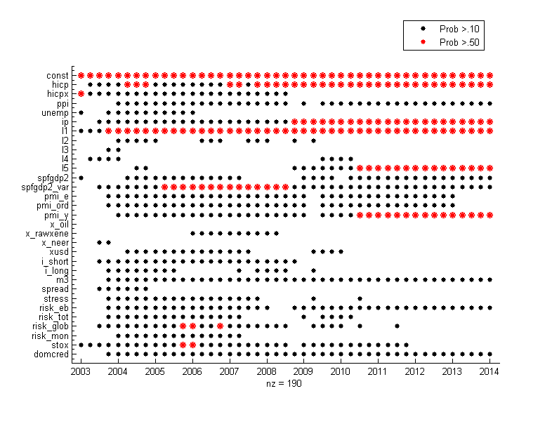
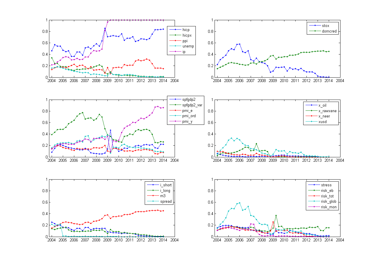
The inclusion probabilities identify which were the most useful indicators of real activity and how this changed over time. In more detail:

• Lags of GDP were, as expected, important overall. The first lag captures the persistence in GDP, and it remained important even during the crisis, when GDP showed pronounced swings. The fourth and fifth lag capture essentially base effects. Our decision to include lag 5 as a potential regressor turned out to be justified.

• Among the consumer price variables, HICP was an important regressor over the whole sample. This confirms the idea that prices and output are not determined in isolation. Without extending our interpretation to the existence of a European Phillips curve, we notice that these results confirms the results for the euro area recently obtained by Giannone et al. (2014). Furthermore, the DMA emphasized the role of producer prices as a forward-looking indicator for nowcasting GDP.

• Among the early indicators of real activity, industrial production was the most important. This is a well known result in nowcasting, where industrial production is widely used as a timely and already comprehensive subset of GDP. The role of unemployment changed over time, becoming less important in the aftermath of the crisis.

• DMA selected almost all GDP surveys as important over the sample, with the exception of the period immediately following the 2008 crisis, which the surveys fail to capture adequately. This results confirm the literature on nowcasting inflation (Ang et al., 2007), arguing that surveys have a relevant nowcasting power, thereby supporting the importance of expectations in determining macroeconomic outcomes.

• No single external variable alone had a determinant role. This is possibly due to the relative compactness of the euro area. Even variables traditionally important in determining prices, such as oil prices or the exchange rate, appear to have had a limited impact on real GDP. We find this result interesting but not surprising, given that these variables mostly affect prices, and affect GDP only indirectly.

• Among the variables closer to the operation of monetary policy, interest rates progressively lost their importance in the credit constrained post-crisis period, while the monetary variable M3 had an increasing role, possibly highlighting the importance of liquidity in the recent part of the sample.

• Risk variables were useful predictors for GDP. Almost all risk indicators seemed to matter before the crisis, in particular the indicator of global risk. The indicator of financial and banking risk remained important during the crisis.

Koop and Onorante (2014) carried out a similar analysis of inflation. They used DMA on a similar dataset, but they explored the whole model space, which limited the number of predictor variables they could use. Comparing their results with ours, it is apparent that the determinants of GDP growth were fairly similar to those of inflation. The differences are largely intuitive: while cycle variables influence consumer prices, GDP is also well forecasted with producer prices, determined in advance; international prices do not have the same importance for the cycle as they have for inflation. On the other hand, as in Koop and Onorante (2014), variables representing expectations are important predictors, with the exception of the crisis period.

A natural complement to the results above is the average sizes of the coefficient of each variable. These are shown in Figure 5. While inclusion probabilities provide important information about which variables should be included in the regressions at each point in time (as a significance test would do), they do not specify the size of their effect, and even a variable with a very high inclusion probability may have a small overall impact on GDP. The coefficients are averages over models at each point in time, and so vary over time.

Figure 5: Posterior Means of Regression Coefficients Over Time Under DMA.

5 Sensitivity Analysis

5.1 Initial conditions

The DOW method requires the specification of an initial set of models at the first time point. In our implementation we used an initial set consisting of just one model, the constant model with no regressors, or null model. In this section we check the sensitivity of the forecast to the choice of the initial population of models.

Figure 6 reports the average number of variables included in the models. The same average size of models is a necessary but not sufficient condition for convergence in populations of models, but it allows an easy graphic exploration of convergence.

Figure 6: Evolution of average model size starting from different initial model populations: one single model (the constant) or a random population of 100 models of average size 8

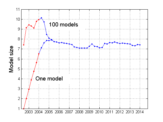
It appears that DMA favours models with about 7-8 variables, and that the initial population $M_{0}$ is not representative of the final models selected. Figure 3 supports this finding by showing that the inclusion probabilities change rapidly at the beginning of the sample. Beyond the few periods of presample (in red) and a few initial points, two very different initial conditions: 1) an initial population of a model only, including only the constant, and 2) with a random population of 100 models, give very comparable results both in terms of model size (Figure 6) and forecasting power.

Table 3 compares the forecasting performance of different methods with various flavours of DMA and DMS, staring with a random initial population of models with average size 8. The results are very similar to those in Table 2, in which DMA was initialized with the null model only. Once again, the DMA methods outperformed the others considered.

Table 3: Forecasting Results Starting From an Initial Population of Models of Average Size 8. The best performers under each criterion are shown in bold.

	RW	AR2	DMA-R	DMA-E	DMS-R	DMS-E
RMSE	0.0101	0.0088	0.0043	0.0043	0.0047	0.0047
MAE	0.0067	0.0059	0.0032	0.0032	0.0035	0.0035
MAX	0.0332	0.0376	0.0127	0.0127	0.0139	0.0139

5.2 Maximum number of models

A pure application of the Occam’s window principle and of the FEAR algorithm would require each model to satisfy condition (3). This would soon lead to a relatively high number of models in the wider population $M_{1}$, as this population, generated from the Expand step of the algorithm, includes all possible neighbours of the preceding population $M_{0}$. The latter, however, is comparatively well contained by the following Reduce step, where condition (3) is applied. Figure 7 shows the evolution of the size of population $M_{0}$ over time.

Figure 7: Occam’s window and number of models over time: $M_{0}$

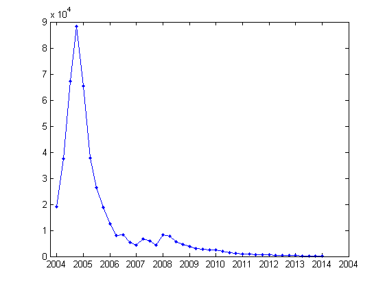
The effort of the algorithm to find a stable population of models at the beginning is reflected in the high number of models retained. It is important to note that we start our evaluation sample after ten data points; as a result many models are poorly estimated at first and their performance varies considerably. After a few periods, a stable population has been found and it is progressively refined; as a result the size of $M_{0}$ decreases.

Starting from a valid population, as in our hypothesis, the FEAR algorithm increases the population size only during turbulent times, for example at the beginning of the Great Recession in 2008-2009. The algorithm automatically increases the population $M_{0}$ because the forecast is less accurate and no model is clearly dominating. This leads the FEAR algorithm to “resuscitate” additional models in the attempt to improve the forecast. Figure 7 shows that this attempt is usually successful. Quiet periods are instead characterized by smaller, stable model populations.

Finally, as the sample size increases and models including the best regressors are selected the necessary population size becomes quite small (the last $M_{0}$ had size 186). Overall, the population $M_{0}$, from which the baseline nowcast is generated, never exceeded 10,000 models, while the wider $M_{1}$ can be up to about ten times larger.

In the interest of speed, we introduced the possibility of specifying a maximum number of models $N$, and our last sensitivity analysis experiments with this number in order to assess whether it implies a deterioration of the forecast. Figure 8 reports the nowcasting performance (as measured by the RMSE) in relation to maximum model size N.

Figure 8: Number of models and RMSE of nowcasting

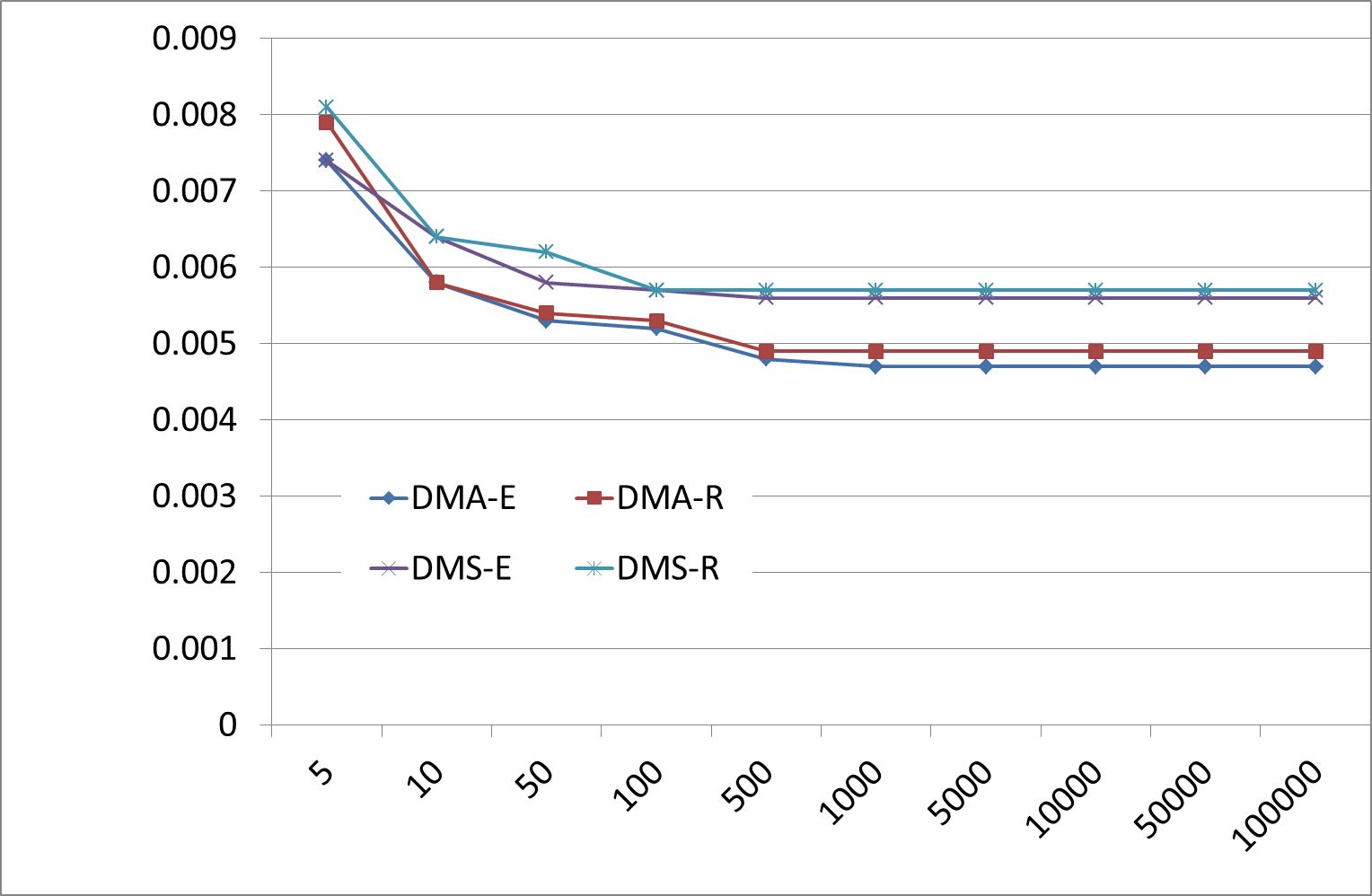
In our model space of 27 potential regressors, forecasting performance improved until about 10,000 models in the population $M_{0}$. Bigger model populations do not lead to any further improvement, as we have seen from the unconstrained estimation, and constraints set at 50,000 or above on the total population are not binding and thus exactly equivalent to Occam’s window without a maximum number of models. We would of course still recommend keeping the maximum number of models as high as possible.

Figure 8 also confirms that in our case DMA performs slightly better than DMS for any population size. This is a robust result in the case of macroeconomic variables, but it cannot be generalized. Koop and Onorante (2014) and Morgan et al. (2014), for example, have shown using Google searches as predictors that DMS performed better in contexts where the data were noisy and forecasting benefitted from excluding many regressors.

When looking at specific parameter values we observe that convergence may be slower for those parameters characterized by low inclusion probabilities. For some specific parameters and inclusion probabilities there are observable convergence issues up to 50,000 models. When this more specific information is important, we would suggest increasing the maximum number of models by one (or if possible two) orders of magnitude.

6 Conclusions

We have proposed a new method for carrying out Dynamic Model Averaging when the model space is too large to allow exhaustive evaluation, so the original DMA method of Raftery et al. (2010) is not feasible. This method, based on Occam’s window and called Dynamic Occam’s Window (DOW), is particularly efficient in situations in which numerous time series of limited length are available, as is typically the case in macroeconomics. Our procedure allows us to perform Dynamic Model Averaging without considering the whole model space but using a subset of models and dynamically optimizing the choice of models at each point in time.

We tested the model in an important empirical application, nowcasting GDP in the euro area. We showed that the forecasting performance was satisfactory compared to common benchmarks and that the results compare well with recent literature and with estimations performed on similar data sets. Several sensitivity analyses confirm the robustness of our approach to the choice of the user-specified control parameters.

Acknowledgements:

Raftery’s research was supported by NIH grants R01 HD054511 and R01 HD070936 and by a Science Foundation Ireland E.T.S. Walton visitor award, grant reference 11/W.1/I2079. Raftery thanks the School of Mathematical Sciences at University College Dublin for hospitality during the preparation of this article.

References

- Ang et al. (2007) Ang, A., G. Bekaert, and M. Wei (2007). Do macro variables, asset markets, or surveys forecast inflation better? Journal of Monetary Economics 54, 1163–1212.
- Brock and Durlauf (2001) Brock, W. and S. N. Durlauf (2001). Growth empirics and reality. World Bank Economic Review 15, 229–272.
- Brock et al. (2003) Brock, W., S. N. Durlauf, and K. West (2003). Policy evaluation in uncertain economic environments. Brookings Papers on Economic Activity 1, 235–322.
- Durlauf et al. (2006) Durlauf, S. N., A. Kourtellos, and C. M. Tan (2006). Is God in the details? a reexamination of the role of religion in economic growth. Working paper, University of Wisconsin.
- Durlauf et al. (2008) Durlauf, S. N., A. Kourtellos, and C. M. Tan (2008). Are any growth theories robust? Economic Journal 118, 329–346.
- Eicher et al. (2010) Eicher, T., C. Papageorgiou, and A. E. Raftery (2010). Determining growth determinants: Default priors and predictive performance in Bayesian model averaging. Journal of Applied Econometrics 26, 30–55.
- Fernández et al. (2001) Fernández, C., E. Ley, and M. F. J. Steel (2001). Benchmark priors for Bayesian model averaging. Journal of Econometrics 100, 381–427.
- Fernández and Steel (2001) Fernández, C. and M. F. J. Steel (2001). Model uncertainty in cross-country growth regressions. Journal of Applied Econometrics 16, 563–576.
- Giannone et al. (2014) Giannone, D., M. Lenza, D. Momferatou, and L. Onorante (2014). Short-term inflation projections: A Bayesian vector autoregressive approach. International Journal of Forecasting 30, 635–644.
- Hoeting et al. (1999) Hoeting, J. A., D. Madigan, A. E. Raftery, and C. T. Volinsky (1999). Bayesian model averaging: A tutorial. Statistical Science 14, 382–417.
- Koop and Korobilis (2012) Koop, G. and D. Korobilis (2012). Forecasting inflation using dynamic model averaging. International Economic Review 53, 867–886.
- Koop and Onorante (2014) Koop, G. and L. Onorante (2014). Macroeconomic nowcasting using Google probabilities. Mimeo, August 2014.
- Leamer (1978) Leamer, E. E. (1978). Specification Searches: Ad Hoc Inference with Nonexperimental Data. New York: Wiley.
- Ley and Steel (2007) Ley, E. and M. F. J. Steel (2007). Jointness in Bayesian variable selection with applications to growth regression. Journal of Macroeconomics 29, 476–493.
- Ley and Steel (2009) Ley, E. and M. F. J. Steel (2009). On the effect of prior assumptions in BMA with applications to growth regression. Journal of Applied Econometrics 24, 651–674.
- Madigan and Raftery (1994) Madigan, D. and A. E. Raftery (1994). Model selection and accounting for model uncertainty in graphical models using Occam’s window. Journal of the American Statistical Association 89, 1535–1546.
- Morgan et al. (2014) Morgan, J., S. Muzikarova, and L. Onorante (2014). Nowcasting European unemployment using Internet search data. Mimeo, August 2014.
- Raftery (1988) Raftery, A. E. (1988). Approximate Bayes factors for generalized linear models. Technical Report 121, Department of Statistics, University of Washington.
- Raftery (1995) Raftery, A. E. (1995). Bayesian model selection for social research. Sociological Methodology 25, 111–163.
- Raftery et al. (2010) Raftery, A. E., M. Kárný, and P. Ettler (2010). Online prediction under model uncertainty via Dynamic Model Averaging: Application to a cold rolling mill. Technometrics 52, 52–66.
- Raftery et al. (1997) Raftery, A. E., D. Madigan, and J. A. Hoeting (1997). Bayesian model averaging for linear regression models. Journal of the American Statistical Association 92, 179–191.
- Sala-i-Martin et al. (2004) Sala-i-Martin, X., G. Doppelhofer, and R. I. Miller (2004). Determinants of long-term growth: A Bayesian averaging of classical estimates (BACE) approach. American Economic Review 94, 813–835.
- Steel (2011) Steel, M. F. J. (2011). Bayesian model averaging and forecasting. Bulletin of E.U. and U.S. Inflation and Macroeconomic Analysis 200, 30–41.
- Varian (2014) Varian, H. R. (2014). Big data: new tricks for econometrics. Journal of Economic Perspectives 28, 3–28.