Re-examination of Large Scale Structure
& Cosmic Flows

Abstract

Comparison of galaxy flows with those predicted from the local galaxy distribution ended as an active field after two analyses came to vastly different conclusions 25 years ago, but that was due to faulty data. All the old results are therefore suspect. With new data collected in the last several years, the problem deserves another look. For this we analyze the gravity field inferred from the enormous data set derived from the 2MASS collection of galaxies (Huchra et al., 2005), and compare it to the velocity field derived from the well calibrated SFI++ Tully-Fisher catalog (Springob et al., 2007). Using the ”Inverse Method” to minimize Malmquist biases, within 10,000 km/s the gravity field is seen to predict the velocity field (Davis et al., 2011) to remarkable consistency. This is a beautiful demonstration of linear perturbation theory and is fully consistent with standard values of the cosmological variables.

1 Comparison of Observed Velocity Field with Gravitational Field

This is a conference proceeding where I summarize several recent publications on peculiar velocities. In particular the brief discussion is based on Davis et al. (2011) (hereafter D11), Nusser & Davis (1994) (hereafter ND94), and Davis et al. (1996) (hereafter DNW96). Interested parties will find complete references therein.

The analysis of Davis et al. (2011) fits the peculiar velocity field given by the SFI++ Tully-Fisher whole sky sample of 2830 galaxies with redshifts $cz<10,000$ km/s (Springob et al., 2007) to a set of orthogonal polynomials by means of an inverse Tully-Fisher (ITF) procedure. The peculiar velocity field derived from this sample is then compared to the gravity field from the largest whole sky redshift survey, the 2MRS survey (Huchra et al., 2005). This catalog is $K$ band selected 2MASS galaxies and has been extended to 43,500 galaxies to $K\leq 11.75$ and $|b|>5^{\circ}$ or $|b|>10^{\circ}$ near the galactic center. In our lifetime, the redshift catalog and derived gravity field is unlikely to improve enough to bother, since it is not the limiting noise. For improvements in the future, one should work on enlarging the TF data.

Peculiar velocities are unique in that they provide explicit information on the three dimensional mass distribution, and measure mass on scales of $10-60h^{-1}$ Mpc, a scale untouched by alternative methods. Here we will be concerned with a comparison of the observed peculiar velocities on the one hand and the velocities derived from the fluctuations in the galaxy distribution on the other. The basic physical principle behind this comparison is simple. The large scale flows are almost certainly the result of the process of gravitational instability with overdense regions attracting material, and underdense regions repelling material. Initial conditions in the early universe might have been somewhat chaotic, so that the original peculiar velocity field (i.e. deviations from Hubble flow) was uncorrelated with the mass distribution, or even contained vorticity. But those components of the velocity field which are not coherent with the density fluctuations will adiabatically decay as the Universe expands, and so at late times one expects the velocity field to be aligned with the gravity field, at least in the limit of small amplitude fluctuations (Peebles, 1980; Nusser et al., 1991). In the linear regime, this relation implies a simple proportionality between the gravity field g and the velocity field ${\bf v}_{\rm g}$, namely ${\bf v}_{\rm g}\propto{\bf g}~{}t$ where the only possible time $t$ is the Hubble time. The exact expression depends on the mean cosmological density parameter $\Omega$ and is given by Peebles (1980),

$${\bf v}_{\rm g}(r)={\frac{2f(\Omega)}{3H_{0}\Omega}}{\bf g}({\bf r})\ .$$ (1)

Given complete knowledge of the mass fluctuation field $\delta_{\rho}({\bf r})$ over all space, the gravity field ${\bf g(r)}$ is

$${\bf g}({\bf r})=G\bar{\rho}\int d^{3}{\bf r^{\prime}}\delta_{\rho}({\bf r^{\prime}})\frac{{\bf r^{\prime}}-{\bf r}}{|{\bf r^{\prime}}-{\bf r}|^{3}}\ ,$$ (2)

where $\bar{\rho}$ is the mean mass density of the Universe. If the galaxy distribution at least approximately traces the mass on large scale, with linear bias $b$ between the galaxy fluctuations $\delta_{G}$ and the mass fluctuations (i.e. $\delta_{g}=b\delta_{\rho}$), then from (1) and (2) we have

$${\bf v}_{\rm g}(r)={H_{0}\beta\over 4\pi{\bar{n}}}\sum_{i}{1\over\phi(r_{i})}{\bf r_{\rm i}-r\over|r_{\rm i}-r|^{3}}+{{H_{0}\beta}\over 3}{\bf r}\ ,$$ (3)

where $\bar{n}$ is the true mean galaxy density in the sample, $\beta\equiv f(\Omega)/b$ with $f\approx\Omega^{0.55}$ the linear growth factor (Linder, 2005), and where we have replaced the integral over space with a sum over the galaxies in a catalog, with radial selection function $\phi(r)$. The second term is for the uniform component of the galaxy distribution and would exactly cancel the first term in the absence of clustering within the survey volume. Note that the result is insensitive to the value of $H_{0}$, as the right hand side has units of velocity. We shall henceforth quote all distances in units of $\ {\rm km\,s^{-1}}$. The sum in equation (3) is to be computed in real space, whereas the galaxy catalog exists in redshift space. As we shall see in §2, the modified equation, which includes redshift distortions, maintains a dependence on $\Omega$ and $b$ through the parameter $\beta$. Therefore, a comparison of the measured velocities of galaxies to the predicted velocities, ${\bf v}_{\rm g}(r)$, gives us a measure of $\beta$. Further, a detailed comparison of the flow patterns addresses fundamental questions regarding the way galaxies trace mass on large scales and the validity of gravitational instability theory.

2 Methods

In this section we outline our method described in ND94, ND95 and DNW96 for deriving the smooth peculiar velocities of galaxies from an observed distribution of galaxies in redshift space and, independently, from a sample of spiral galaxies with measured circular velocities $\eta$ and apparent magnitudes $m$.

Here we restrict ourselves to large scales where linear-theory is applicable. We will use the method of ND94 for reconstructing velocities from the 2MRS. This method is particularly convenient, as it is easy to implement, fast, and requires no iterations. Most importantly, this redshift space analysis closely parallels the ITF estimate described below. We next present a very brief summary of the methodology.

We follow the notation of DNW96. The comoving redshift space coordinate and the comoving peculiar velocity relative to the Local Group (LG) are, respectively, denoted by $s$$s$$s$ (i.e. $s=cz/H_{0}$) and $\kern-0.24994pt\hbox{$v$}\kern-5.20601pt\kern 0.50003pt\hbox{$v$}\kern-5.20601pt\kern-0.24994pt\raise 0.43304pt\hbox{$v$}(\kern-0.24994pt\hbox{$s$}\kern-4.6875pt\kern 0.50003pt\hbox{$s$}\kern-4.6875pt\kern-0.24994pt\raise 0.43304pt\hbox{$s$})$. To first order, the peculiar velocity is irrotational in redshift space (Chodorowski & Nusser, 1999) and can be expressed as $\kern-0.24994pt\hbox{$v$}\kern-5.20601pt\kern 0.50003pt\hbox{$v$}\kern-5.20601pt\kern-0.24994pt\raise 0.43304pt\hbox{$v$}_{g}(\kern-0.24994pt\hbox{$s$}\kern-4.6875pt\kern 0.50003pt\hbox{$s$}\kern-4.6875pt\kern-0.24994pt\raise 0.43304pt\hbox{$s$})=-\kern-0.24994pt\hbox{$\nabla$}\kern-8.33336pt\kern 0.50003pt\hbox{$\nabla$}\kern-8.33336pt\kern-0.24994pt\raise 0.43304pt\hbox{$\nabla$}\Phi(\kern-0.24994pt\hbox{$s$}\kern-4.6875pt\kern 0.50003pt\hbox{$s$}\kern-4.6875pt\kern-0.24994pt\raise 0.43304pt\hbox{$s$})$ where $\Phi(\kern-0.24994pt\hbox{$s$}\kern-4.6875pt\kern 0.50003pt\hbox{$s$}\kern-4.6875pt\kern-0.24994pt\raise 0.43304pt\hbox{$s$})$ is a potential function. As an estimate of the fluctuations in the fractional density field $\delta_{0}(\kern-0.24994pt\hbox{$s$}\kern-4.6875pt\kern 0.50003pt\hbox{$s$}\kern-4.6875pt\kern-0.24994pt\raise 0.43304pt\hbox{$s$})$ traced by the discrete distribution of galaxies in redshift space we consider,

$$\delta_{0}(\kern-0.24994pt\hbox{$s$}\kern-4.6875pt\kern 0.50003pt\hbox{$s$}\kern-4.6875pt\kern-0.24994pt\raise 0.43304pt\hbox{$s$})={1\over{(2\pi)^{3/2}{\bar{n}}\sigma^{3}}}\sum_{i}{{w(L_{0i})}\over{\phi(s_{i})}}\exp\left[-{{\left(\kern-0.24994pt\hbox{$s$}\kern-4.6875pt\kern 0.50003pt\hbox{$s$}\kern-4.6875pt\kern-0.24994pt\raise 0.43304pt\hbox{$s$}-\kern-0.24994pt\hbox{$s$}\kern-4.6875pt\kern 0.50003pt\hbox{$s$}\kern-4.6875pt\kern-0.24994pt\raise 0.43304pt\hbox{$s$}_{i}\right)^{2}}\over{2\sigma^{2}}}\right]-1\quad.$$ (4)

where $\bar{n}=\sum_{i}w(L_{0i})/\phi(s_{i})$ and $w$ weighs each galaxy according to its estimated luminosity, $L_{0i}$. The 2MRS density field is here smoothed by a gaussian window with a redshift independent width, $\sigma=350\ {\rm km\,s^{-1}}$. This is in contrast to DNW96 where the IRAS density was smoothed with a width proportional to the mean particle separation. The reason for adopting a constant smoothing for 2MRS is its dense sampling which is nearly four time higher than IRAS . We emphasize that the coordinates ${\bf s}$ are in observed redshift space, expanded in a galactic reference frame. The only correction from pure redshift space coordinates is the collapse of the fingers of god of the known rich clusters prior to the redshift space smoothing (Yahil et al. 1991). Weighting the galaxies in equation (4) by the selection function and luminosities evaluated at their redshifts rather than the actual (unknown) distances yields a biased estimate for the density field. This bias gives rise to Kaiser’s rocket effect (Kaiser, 1987).

To construct the density field, equation 4, we volume limit the 2MRS sample to 3000 km/s, so that $\phi{(s<3000)}=1$, resulting in $\phi{(s=10000)}=0.27$ (Westover, 2007). In practice, this means we delete galaxies from the 2MRS sample fainter than $M_{*}+2$. Galaxies at 10,000 km/s therefore have $1/\phi=3.7$ times the weight of foreground galaxies in the generation of the velocity field, $v_{g}$.

If we expand the angular dependence of $\Phi$ and $\delta_{0}(\kern-0.24994pt\hbox{$s$}\kern-4.6875pt\kern 0.50003pt\hbox{$s$}\kern-4.6875pt\kern-0.24994pt\raise 0.43304pt\hbox{$s$})$ redshift space in spherical harmonics in the form,

$$\Phi(\kern-0.24994pt\hbox{$s$}\kern-4.6875pt\kern 0.50003pt\hbox{$s$}\kern-4.6875pt\kern-0.24994pt\raise 0.43304pt\hbox{$s$})=\sum_{l=0}^{\infty}\sum_{m=-l}^{l}\Phi_{lm}(s)Y_{lm}(\theta,\varphi)$$ (5)

and similarly for $\delta_{0}$, then, to first order, $\Phi_{lm}$ and $\delta_{0lm}$ satisfy,

$${1\over{s^{2}}}{{\rm d}\over{{\rm d}s}}\left(s^{2}{{{\rm d}\Phi_{lm}}\over{{\rm d}s}}\right) - {1\over{1+\beta}}{{l(l+1)\Phi_{lm}}\over{s^{2}}}$$

$$= {\beta\over{1+\beta}}\left(\delta_{0lm}-{\kappa(s)}{{{\rm d}\Phi_{lm}}\over{{\rm d}s}}\right)\;,$$

where

$$\kappa=\frac{{\rm d}{\rm ln}\phi}{{\rm d}s}-\frac{2}{s}\frac{d{\rm ln}w(L_{0i})}{d{\rm ln}L_{0i}}$$ (7)

represents the correction for the bias introduced by the generalized Kaiser rocket effect. As emphasized by ND94, the solutions to equation (2) for the monopole ($l=0$) and the dipole ($l=1$) components of the radial peculiar velocity in the LG frame are uniquely determined by specifying vanishing velocity at the origin. That is, the radial velocity field at redshift $\bf s$, when expanded to harmonic $l\leq 1$, is not influenced by material at redshifts greater than $\bf s$.

In this paper, we shall consider solutions as a function of $\beta$. Davis et al. (2011) also fit a second parameter, $\alpha$, defining a power law form $w_{i}\propto L_{i}^{\alpha}$ for the galaxy weights and found $\alpha\approx 0$ was the best fit. The large-scale gravity field is best estimated if all the galaxies are equal-weighted, that is, they all have the same mass. This makes sense if you remember that each point in the 2MRS represents the mass on scales of $\sim 4$ Mpc.

3 Generating Peculiar Velocities

Given a sample of galaxies with measured circular velocity parameters, $\eta_{i}\equiv{\rm log}\omega_{i}$, linewidth $\omega_{i}$, apparent magnitudes $m_{i}$, and redshifts $z_{i}$, the goal is to derive an estimate for the smooth underlying peculiar velocity field. We assume that the circular velocity parameter, $\eta$, of a galaxy is, up to a random scatter, related to its absolute magnitude, $M$, by means of a linear inverse Tully-Fisher (ITF) relation, i.e.,

$$\eta=\gamma M+\eta_{0}.$$ (8)

One of the main advantages of inverse TF methods is that samples selected by magnitude, as most are, will be minimally plagued by Malmquist bias effects when analyzed in the inverse direction (Schechter, 1980; Aaronson et al., 1982). We write the absolute magnitude of a galaxy,

$$M_{i}=M_{0i}+P_{i}$$ (9)

where

$$M_{0i}=m_{i}+5{\rm log}(z_{i})-15$$ (10)

and

$$P_{i}=5{\rm log}(1-u_{i}/z_{i})$$ (11)

where $m_{i}$ is the apparent magnitude of the galaxy, $z_{i}$ is its redshift in units of $\ {\rm km\,s^{-1}},$ and $u_{i}$ its radial peculiar velocity in the LG frame.

4 The Solution in Orthogonal Polynomials

Functions based on $Y_{lm}$ are a poor description.of the complex flows of LSS, giving rise to correlated residuals, but with only $\sim 20$ numbers to describe the field, we get $\chi^{2}/{\rm dof}=1$ when we compare the gravity and velocity fields; 25 years ago, the same comparison gave $\chi^{2}/{\rm dof}=2$ (Davis et al., 1996). In the interval, the IRAS gravity field has been replaced by the 2MRS, but the two gravity fields are essentially identical. The TF data has been updated to the SFI++ catalogue, which makes all the difference; the old data was constructed of 4 separate catalogues and it was not uniformly calibrated.

The choice of radial basis functions for the expansion of the modes can be made with considerable latitude. The functions should obviously be linearly independent, and close to orthogonal when integrated over volume. They should be smooth and close to a complete set of functions up to a given resolution limit. Spherical harmonics and radial Bessel functions are an obvious choice, but Bessel functions have a constant radial resolution with distance whereas the measured peculiar velocities have velocity error that scales linearly with distance. We deal with this problem by choosing to make the Bessel functions a function of $y$ instead of $r$ by means of the transformation

$$y(r)=({\rm log}(1+(r/r_{s}))^{1/2}$$ (12)

where $r_{s}=5000$ km/s. The resulting radial functions oscillate more rapidly toward the origin then they do toward the outer limit, a physically desirable behavior.

5 The Resulting Velocity and Gravity Fields

Figure 1: The derived peculiar velocities ${\bf v_{{}_{\rm itf}}}$ and $g$$g$$g$ of SFI++ galaxies on aitoff projections on the sky in galactic coordinates. Red points have positive peculiar velocity and blue points have negative. The rows correspond to galaxies with $cz<2000$, $2000<cz<4000$ $4000<cz<6000\ {\rm km\,s^{-1}}$ and $6000<cz<10000$ km/s, respectively. The size of the symbols is linearly proportional to the velocity amplitude (see key to the size of the symbols given at the bottom of the figure). In order to better see the differences, a 400 km/s dipole, in the direction of the CMB dipole, has been subtracted from the ${\bf v_{{}_{\rm itf}}}$ and $g$$g$$g$ velocities.

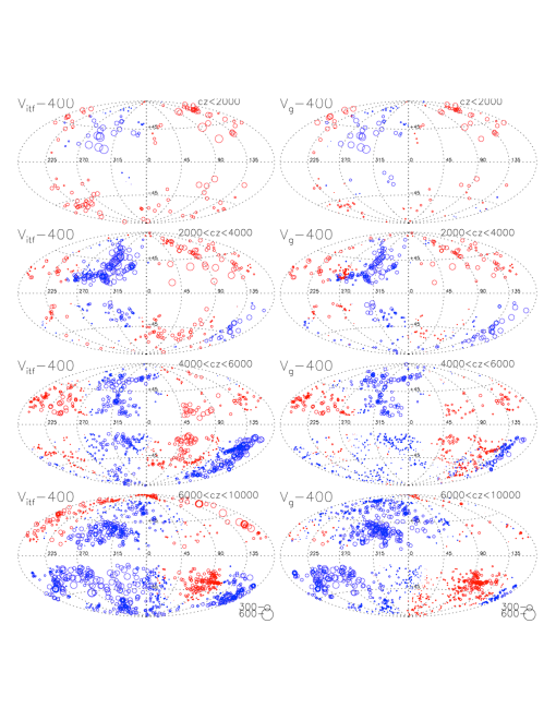
In the aitoff projections in Figure 1 we plot the TF peculiar velocities of the SFI++ galaxies, $\bf v_{{}_{\rm itf}}$ and the derived gravity modes, $g$$g$$g$ , for galaxies in redshift shells, $cz<2000$, $2000<cz<4000$, $4000<cz<6000$, and $6000<cz<10000$ km$s^{-1}$. The projections are in galactic coordinates centered on l,b = 0 and with $b=90$ at the top. Figure 1 is shown with $\beta=0.35$; the amplitude of $g$$g$$g$ is almost linear with $\beta$, giving a powerful diagnostic. Our best fit is $\beta=0.33\pm 0.04$. The key point is to note that the residuals are small for the entire sky and have amplitude that is constant with redshift. The amplitude and coherence of the residuals ${\bf v_{{}_{\rm itf}}}-\kern-0.24994pt\hbox{$g$}\kern-5.12846pt\kern 0.50003pt\hbox{$g$}\kern-5.12846pt\kern-0.24994pt\raise 0.43304pt\hbox{$g$}$ is the same as for the mock catalogs in figure 2, where for example the lower picture shows ${\bf v_{{}_{\rm itf}}}-\kern-0.24994pt\hbox{$g$}\kern-5.12846pt\kern 0.50003pt\hbox{$g$}\kern-5.12846pt\kern-0.24994pt\raise 0.43304pt\hbox{$g$}$ for real and mock catalogs. The mocks show the viability of the full procedure (Davis et al., 2011).

Figure 1 says it all – the agreement between the inferred velocity field and the gravitational expectations is spectacularly good at all distances. These two fields could have been very discrepant; the only parameter of the fitting is $\beta$. The flow field is complex, as galaxies respond to their local gravity field. All the argumentation of 25 years ago is irrelevant. Note that we are only using 20 numbers to describe the local field, thus smoothing out the small scale velocity field.

5.1 Residual Velocity Correlations

Figure 2: Top: The velocity correlation of the real data and 15 mock catalogs. The dashed red and solid red curves curve are, respectively, the correlations of $v_{{}_{\rm itf}}$ and ${\bf v_{{}_{\rm itf}}}-\kern-0.24994pt\hbox{$g$}\kern-5.12846pt\kern 0.50003pt\hbox{$g$}\kern-5.12846pt\kern-0.24994pt\raise 0.43304pt\hbox{$g$}$ in the real data. This plot shows that the 20 mode expansion removes virtually the entire velocity field. The blue lines are each correlations of $v_{{}_{\rm itf}}-\kern-0.24994pt\hbox{$g$}\kern-5.12846pt\kern 0.50003pt\hbox{$g$}\kern-5.12846pt\kern-0.24994pt\raise 0.43304pt\hbox{$g$}$ for the mock catalogs. Bottom: Velocity correlations for 15 mock catalogs. The red curves are the velocity of ${\bf v_{itf}}$, the dot-dashed curves show the correlation of ${\bf(v_{true}-v_{g})}$, and the blue curves correspond to ${\bf v_{true}-v_{itf})}$. Both ${\bf v_{true}}$ and ${\bf v_{g}}$ are first smoothed with the 20 mode expansion before the autocovariance is computed. Note that the correlation of ${\bf v_{{}_{\rm itf}}}-\kern-0.24994pt\hbox{$g$}\kern-5.12846pt\kern 0.50003pt\hbox{$g$}\kern-5.12846pt\kern-0.24994pt\raise 0.43304pt\hbox{$g$}$ is only slightly worse than the correlation of ${\bf v_{true}-v_{gs}}$, showing that the velocity reconstruction dominates the errors. Note also that we are plotting the square root of the velocity correlation $\Psi$.

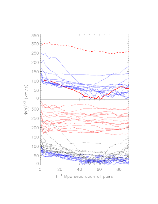
The residuals, both in the real and mock data, have error fields, ${\bf v_{{}_{\rm itf}}}-\kern-0.24994pt\hbox{$g$}\kern-5.12846pt\kern 0.50003pt\hbox{$g$}\kern-5.12846pt\kern-0.24994pt\raise 0.43304pt\hbox{$g$}$, that show large regions of coherence. To address the significance of these errors, we show in figure 2 the velocity correlation function (Gorski et al., 1989) defined as

$$\Psi(s;{u})=\frac{\sum_{pairs}u_{1}u_{2}{\rm cos}\theta_{12}}{\sum_{pairs}{\rm cos}^{2}\theta_{12}}$$ (13)

where the sum is over all pairs, 1 and 2, separated by vector distance $\bf s_{12}$ (in redshift space), ${\rm\theta_{12}}$ is the angle between points $1$ and $2$, and $u$ is either $v_{{}_{\rm itf}}$ (dashed red) or ${\bf v_{{}_{\rm itf}}}-\kern-0.24994pt\hbox{$g$}\kern-5.12846pt\kern 0.50003pt\hbox{$g$}\kern-5.12846pt\kern-0.24994pt\raise 0.43304pt\hbox{$g$}$ (red for data, blue for 15 mock catalogs), At small lags for the real data, the function $\Psi(r;{\bf v_{{}_{\rm itf}}}-\kern-0.24994pt\hbox{$g$}\kern-5.12846pt\kern 0.50003pt\hbox{$g$}\kern-5.12846pt\kern-0.24994pt\raise 0.43304pt\hbox{$g$})$ is a factor of 3 less than $\Psi(s;{\bf v_{{}_{\rm itf}}})$, about the same as for the mock catalogs. Note how the large coherence of ${\bf v_{{}_{\rm itf}}}$ is enormously diminished in $\Psi(s>2000{\rm km/s};{\bf v_{{}_{\rm itf}}}-\kern-0.24994pt\hbox{$g$}\kern-5.12846pt\kern 0.50003pt\hbox{$g$}\kern-5.12846pt\kern-0.24994pt\raise 0.43304pt\hbox{$g$})$. This shows that the coherence seen in the residual field, figure 2, is expected and is not a problem. The large scale drift of a sample is demonstrated by the persistent amplitude of $\Psi$ beyond $\approx 60-80$ Mpc.

The bottom panel of figure 2 shows velocity correlations for 15 mock catalogs where the actual velocity ${\bf v_{true}}$ generated in the nbody code and then smoothed with the 20 mode expansion can be compared to either ${\bf v_{{}_{\rm itf}}}$ or $g$$g$$g$. Note that the raw velocities, ${\bf v_{itf}}$ (red), have enormous correlation that reaches large lag, while the correlations, $({\bf v_{true}-v_{{}_{\rm itf}}})$, (blue) are extremely small. This is because the only difference with $v_{true}$ is the gaussian error in $\Delta\eta=.05$ that affects ${\bf v_{{}_{\rm itf}}}$. The blue curves show this error is not a problem, because the mode expansions are insensitive to gaussian noise in the 2500 galaxies, i.e. they are essentially perfect. This demonstrates that even though the TF noise is as large as for the actual data, the ability to find the correct flow, when characterized by only 20 numbers, is intact.

This demonstrates that the description of the full velocity field by the specification of 20 numbers, specifying the amplitude of the modes, is essentially complete.

6 Summary

• We see no evidence that the dark matter does not follow the galaxy distribution, and it is consistent with constant bias on large scales. There is no evidence for a non-linear bias in the local flows. A smooth component to the universe is not something testable with these methods.

• Linear perturbation theory appears to be adequate for the large scales tested by our method; the comparison of ${\bf v_{p}}$ and ${\bf g}$ is so precise as to be a stunning example of the power of linear theory!

• Our estimate of $\sigma_{8}$ gives the most precise value at $z\sim 0$ and is useful for tests of the growth rate and Dark Energy.

• The velocity-gravity comparison measures the acceleration on scales in the range $10-60$ Mpc. and since we derived a similar value of $\beta$ as for clusters of galaxies, we conclude that dark matter appears to fully participate in the clustering on scales of a few Megaparsecs and larger.

• We find no evidence for large-scale flows, and the small residuals are completely consistent with LCDM (Nusser et al., 2014). Note that our analysis has not used the CMBR dipole, but we see a velocity field that is fully consistent with the CMBR dipole radiation. We see no evidence that the dipole in the CMBR is produced by anything other than our motion in the universe.

• The field of Large Scale Flows, apart from going deeper with TF data, appears to this observer to have finally reached its original goal. Remember that 25 years ago, there were no CMBR results measuring $\Omega_{m}$, and the large scale flows were going to give us the long-sought answer. But the TF data of 25 years ago was not well calibrated and gave inconsistent results, so we lost ground. Now we can state that the LS flows are consistent with standard parameters.

• This finishes the study of the local velocity field, and now I can retire!

References

- Aaronson et al. (1982) Aaronson, M., Huchra, J., Mould, J., Schechter, P. L., & Tully, R. B. 1982, ApJ, 258, 64
- Chodorowski & Nusser (1999) Chodorowski, M. J., & Nusser, A. 1999, MNRAS, 309, L30
- Davis et al. (2011) Davis, M., Nusser, A., Masters, K. L., Springob, C., Huchra, J. P., & Lemson, G. 2011, MNRAS, 413, 2906
- Davis et al. (1996) Davis, M., Nusser, A., & Willick, J. A. 1996, ApJ, 473, 22
- Gorski et al. (1989) Gorski, K. M., Davis, M., Strauss, M. A., White, S. D. M., & Yahil, A. 1989, ApJ, 344, 1
- Huchra et al. (2005) Huchra, J., Jarrett, T., Skrutskie, M., Cutri, R., Schneider, S., Macri, L., Steining, R., Mader, J., Martimbeau, N., & George, T. 2005, in Astronomical Society of the Pacific Conference Series, Vol. 329, Nearby Large-Scale Structures and the Zone of Avoidance, ed. A. P. Fairall & P. A. Woudt, 135–+
- Kaiser (1987) Kaiser, N. 1987, MNRAS, 227, 1
- Linder (2005) Linder, E. V. 2005, Physical Review D., 72, 043529
- Nusser & Davis (1994) Nusser, A., & Davis, M. 1994, ApJL, 421, L1
- Nusser et al. (1991) Nusser, A., Dekel, A., Bertschinger, E., & Blumenthal, G. R. 1991, ApJ, 379, 6
- Nusser et al. (2014) Nusser, A., Davis, M., & Branchini, E. 2014, ApJ, 788, 157
- Peebles (1980) Peebles, P. J. E. 1980, The large-scale structure of the universe (Princeton University Press)
- Schechter (1980) Schechter, P. L. 1980, Astronomical Journal, 85, 801
- Springob et al. (2007) Springob, C. M., Masters, K. L., Haynes, M. P., Giovanelli, R., & Marinoni, C. 2007, ApJ. S, 172, 599
- Westover (2007) Westover, M. 2007, PhD thesis, Harvard University
- Yahil et al. (1991) Yahil, A., Strauss, M. A., Davis, M., & Huchra, J. P. 1991, ApJ, 372, 380