Tail approximations for the Student $t$-, $F$-, and Welch statistics for non-normal and not necessarily i.i.d. random variables

Abstract

Let $T$ be the Student one- or two-sample $t$-, $F$-, or Welch statistic. Now release the underlying assumptions of normality, independence and identical distribution and consider a more general case where one only assumes that the vector of data has a continuous joint density. We determine asymptotic expressions for $\mathbf{P}(T>u)$ as $u\to\infty$ for this case. The approximations are particularly accurate for small sample sizes and may be used, for example, in the analysis of High-Throughput Screening experiments, where the number of replicates can be as low as two to five and often extreme significance levels are used. We give numerous examples and complement our results by an investigation of the convergence speed – both theoretically, by deriving exact bounds for absolute and relative errors, and by means of a simulation study.

1 Introduction

This article extends early results of Bradley [1] and Hotelling [9] on the tails of the distributions of some popular and much used test statistics. We quantify the effect of non-normality, dependence, and non-homogeneity of data on the tails of the distribution of the Student one- and two-sample $t$-, $F$- and Welch statistics. Our approximations are valid for samples of any size, but are most useful for very small sample sizes, for example, when standard central limit theorem-based approximations are inapplicable.

1.1 Problem statement and main result

Let $\mathbf{X}\in\mathbb{R}^{n}$, $n\geq 2$, be a random vector and $T=T_{n}(\mathbf{X})$ be (i) the Student one-sample $t$-test statistic; or (ii) the Student two-sample $t$-test statistic; or (iii) the $F$-test statistic for comparison of variances (in fact the $F$-test results apply also to one-way ANOVA, factorial designs, a lack-of-fit sum of squares test, and an $F$-test for comparison of two nested linear models).

In this paper, we study the asymptotic behavior of the tail distribution of $T$ for small and fixed sample sizes. Let $g_{0}(\mathbf{x})$ be the true joint density of $\mathbf{X}$ under $H_{0}$ and $g_{1}(\mathbf{x})$ be the density under the alternative $H_{1}$. Define $\mathcal{G}$ as a set of continuous densities that satisfy the regularity constraints of Theorems 2.1, 3.1, or 5.1 for the three test statistics accordingly. Our main result is the following theorem.

Theorem 1.1

For any fixed value of $n$ and each of the three choices of $T$, there exists a functional $K\mathchoice{\nobreak\,\colon}{\nobreak\,\colon}{\nobreak\,\colon\;}{\nobreak\,\colon\;}\mathcal{G}\rightarrow\mathbb{R}^{+}$, such that for all $g_{0},g_{1}\in\mathcal{G}$ the limit expression

$$\frac{\mathbf{P}({T>u|H_{1}})}{\mathbf{P}({T>u|H_{0}})}=\frac{K_{g_{1}}}{K_{g_{0}}}+\mathrm{o}(1)\qquad\mbox{as }u\to\infty$$ (1)

holds with constants $0<K_{g_{0}}=K(g_{0})<\infty$ and $0<K_{g_{1}}=K(g_{1})<\infty$. The exact expressions for $K(g)$ are given in (4), (3) and (18) for the three choices of the test statistic $T$.

Remark 1.

Standard assumption in the use of any of the test statistics described above is that $\mathbf{X}\sim\operatorname{MVN}(\mathbf{0},\sigma^{2}\mathbf{1}_{n})$, where $\operatorname{MVN}(\bm{\mu},\bm{\Sigma})$ denote the multivariate normal distribution with mean vector $\bm{\mu}$ and covariance matrix $\bm{\Sigma}$. It is easy to check that $\operatorname{MVN}(\mathbf{0},\sigma^{2}\mathbf{1}_{n})\in\mathcal{G}$ and that $K(\operatorname{MVN}(\mathbf{0},\sigma^{2}\mathbf{1}_{n}))=1$.

Further remarks on Theorem 1.1 are given in Supplementary Materials, see [22].

1.2 Motivation and applications

The questions addressed in this article have gained significant new importance through the explosive increase of High-Throughput Screening (HTS) experiments, where the number of replicates is often small, but instead thousands or millions of tests are performed, at extremely high significance levels. Studying extreme tails of test statistics under deviation from standard assumptions is crucial in HTS because of the following factors:

HTS uses many thousands or even millions of biochemical, genetic or pharmacological tests. In order to get a reasonable number of rejections, the significance level of the tests is often very small, say, 0.001 or lower, and it is the extreme tails of the distribution of test statistics which are important.

HTS assays are often subject to numerous systematic and spatial effects and to large number of preprocessing steps. The resulting data may become dependent, non-normal, or non-homogeneous, yet common test statistics such as one- and two-sample $t$-tests are still routinely computed under standard assumptions.

It is even less likely that the data follows any standard distribution under the alternative hypothesis. By quantifying the tail behavior of a test statistic under arbitrary distributional assumptions, one can get more realistic estimators for the test power.

Given the scale of HTS experiments and necessity to make even larger investments into further research on positives detected through a HTS study, it is important to have realistic picture of the accuracy of such experiments. Consider, for example, estimation of $\mathit{pFDR}$, the positive False Discovery Rate, see Storey [16, 17, 18]. As of now, estimates of $\mathit{pFDR}$ are obtained under the assumption that the true null distribution equals the theoretical one, and this may lead to wrong decisions. In most cases, however, a sample from the null distribution can be obtained by conducting a separate experiment. One can then model the tail distribution of the test statistic, and apply for example, methods of Rootzén and Zholud [14], which account for deviations from the theoretical null distribution.

Due to economical constraints, numbers of replicates in an individual experiment in HTS are as small as two to five, which makes large sample normal approximations inapplicable. Even for moderate sample sizes, CLT-based approximations are not accurate in the tails and better approximations, such as those presented in this paper, are needed.

We now consider a HTS experiment which was the motivation for the present paper. Left panel of Figure 1 shows measured values of the Logarithmic Strain Coefficient (LSC) of the wildtype cells in a Bioscreen array experiment in yeast genome screening studies, see Warringer and Blomberg [19] and Warringer et al. [20].

Figure 1: The wild type data set. Left: Histogram of $3456$ LSC values from the wildtype dataset. Right: Empirical CDF of 1728 $p$-values obtained from one-sample $t$-test for pairs of LSC values.

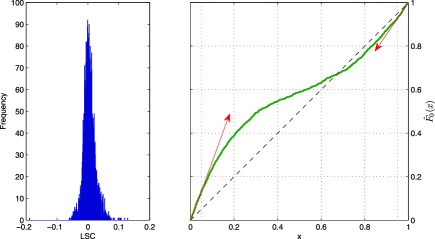
The null hypothesis was that LSC of a wildtype yeast cell had normal distribution with mean zero and unknown variance. The experiment was made for quality control purposes, hence no treatment has been applied and the null hypothesis of mean zero was known to be true.

The histogram of the LSC values was skewed, see Figure 1, and we therefore plotted the empirical cumulative distribution function (CDF) of the $1728$ $p$-values obtained from the LSC values. As expected, see the right panel in Figure 1, the distribution of the $p$-values was different from the theoretical uniform distribution.

Note, however, that both lower and upper tails of the plot approach straight lines, as indicated by the two arrows. This was in fact the starting point of the present article, and it later followed that such tail behavior is justified by Theorem 1.1, see Supplementary Materials.

In practical applications, one needs to be able to compute or estimate the constant $K_{g}$. This can be done in a variety of ways.

For the case when components of $\mathbf{X}$ are i.i.d. random variables, constant $K_{g}$ can be obtained directly from (4), (3) and (18) for the three choices of the test statistic $T$ accordingly. We give numerous examples through Sections 2–5, and Supplementary Materials provides Wolfram Mathematica [11] code to compute $K_{g}$ for even more complicated cases, like, for example, Multivariate Normal case with $g\sim\operatorname{MVN}(\mathbf{0},\bm{\Sigma})$.

For an arbitrary multivariate density $g(\mathbf{x})$ and Student one- and two-sample $t$-statistics, or $F$-statistics with low degrees of freedom, $K_{g}$ can be computed from (4), (3) or (18) using adaptive Simpson or Lobatto quadratures. We provide the corresponding MATLAB [12] scripts in Supplementary Materials.

For an $F$-statistic with the denominator that has more than two degrees of freedom, $K_{g}$ can be computed numerically using Monte Carlo integration, see Supplementary Materials. Monte Carlo methods are applicable to the case described above as well.

The distribution tail of $T$ can be estimated using simulations, see, for example, Section 7. In the current paper we used “brute-force” approach, but importance sampling techniques can be applied quite generally as well.

If $g(\mathbf{x})$ is unknown but one instead has a sample from $g$, then $K_{g}$ can be estimated as a slope of the graph of the CDF of the corresponding $p$-values in the origin of zero. In the yeast genome screening experiment, for example, $K_{g}$ approximately equals the slope of the red arrow – theoretical justification of this fact is given in Supplementary Materials, and the estimation technique is similar to the Peak-Over-Threshold (POT) method in Extreme Value Theory, see, for example, the SmartTail software at www.smarttail.se [15] and further examples in Rootzén and Zholud [14].

Finally, the existence of $K_{g}$ and its importance for questioning the logic behind some multiple testing procedures is discussed in Zholud [21], Part I, Section 3.

1.3 Literature review

There is enormous amount of literature on the behavior of the Student one- and two-sample $t$- and $F$-statistics under deviations from the standard assumptions. The overwhelming part of this literature is focused on normal approximations, that is, when $n\to\infty$. These are large sample approximations though, and are irrelevant to the topic of the present article.

For small and moderate sample sizes, one would typically use Edgeworth expansion, see, for example, Field and Ronchetti [4], Hall [7] and Gaen [5, 6], or saddlepoint approximations, see, for example, Zhou and Jing [23], Jing et al. [10] and Daniels and Young [3]. Edgeworth expansion improves the normal approximation but is still inaccurate in the tails. Saddlepoint approximations, on the other hand, can be very accurate in the tails, see, for example, Jing et al. [10], but the latter statement is based on purely empirical evidence and the asymptotic behavior of these approximations as $u\to\infty$ is not well studied. Furthermore, in practice one would require exact parametric form of the population density, and the use of saddle point approximations in statistical inference is questionable.

As for the approximations considered in this article, that is, when $n$ is small and $u\to\infty$, the existing literature is very limited. This presumably can be explained by the fact that situations where one would need to test at significance levels of $10^{-3}$ and lower never arose, until present times. We focus on the most relevant works by Bradley [1, 2] and Hotelling [9].

Bradley covers the Student one-sample $t$-statistic for i.i.d. non-normal observations, and also makes a somewhat less complete study of the corresponding cases for the Student two-sample $t$-test and the $F$-test of equality of variances. Bradley [2] derives the constant $K_{g}$ from geometrical considerations, but does not state any assumptions on the underlying population density which ensure that the approximations hold. Bradley [1], on the other hand, gives assumptions on the population density, but these assumptions are insufficient, see Section A.2.

Hotelling [9] studies the Student one-sample $t$-test for an “arbitrary” joint density of $\mathbf{X}$. Hotelling derives the constant $K_{g}$ assuming that the limit in the left-hand side of (1) exists and that the function

$$D_{n}(\xi)=\int_{0}^{\infty}r^{n-1}g(r\xi_{1},\ldots,r\xi_{n})\,\mathrm{d}r$$

is continuous for both densities $g_{0}$ and $g_{1}$. When it comes to the examples, however, the existence of the limit in (1) is taken for granted and the assumption of continuity of $D_{n}(\xi)$ is never verified.

Finally, a more detailed literature review that covers other approaches and meritable scientific works is given in Supplementary Materials.

The structure of this paper is as follows: Sections 2–5 contain main theorems and examples; Section 6 addresses the convergence speed and higher order expansions; Section 7 presents a simulation study. Appendix A includes the key lemma used in the proofs, in Section A.1, and a discussion on the regularity conditions, in Section A.2; Appendix B contains figures from the simulation study; and, finally, follows a brief summary of the Supplementary Materials that are available online.

2 One-sample $t$-statistic

Let $\mathbf{X}=(X_{1},X_{2},\ldots,X_{n})$, $n\geq 2$, be a random vector that has a joint density $g$ and define

$$T=\sqrt{n}(\overline{\mathbf{X}}/{S}),$$

where $\overline{\mathbf{X}}$ and $S^{2}$ are the sample mean and the sample variance of the vector $\mathbf{X}$. Introduce the unit vector $\mathbf{I}=(1/{\sqrt{n}},1/{\sqrt{n}},\ldots,1/{\sqrt{n}})$, and assume that

$$g(x\mathbf{I})>0\qquad\mbox{for some }x\geq 0$$ (2)

and that

$$\int_{0}^{\infty}r^{n-1}\mathop{\sup_{\|{\bm{\xi}}\|<\varepsilon,}}_{{\bm{\xi}}\in L^{\bot}}g\bigl{(}r(\mathbf{I}+{\bm{\xi}})\bigr{)}\,\mathrm{d}r<\infty$$ (3)

for some $\varepsilon>0$, where $L$ is the linear subspace of $\mathbb{R}^{n}$ spanned by the vector $\mathbf{I}$ and $L^{\bot}$ is its orthogonal complement. Finally, introduce the constant

$$K_{g}=2\frac{\uppi^{{n}/{2}}}{\Gamma({n}/{2})}\int_{0}^{\infty}r^{n-1}g(r\mathbf{I})\,\mathrm{d}r.$$ (4)

Theorem 2.1

If $g$ is continuous and satisfies (2) and (3), then

$$\frac{\mathbf{P}({T>u})}{t_{n-1}(u)}=K_{g}+\mathrm{o}(1)\qquad\mbox{as }u\to\infty,$$ (5)

where $t_{n-1}(u)$ is the tail of the $t$-distribution with $n-1$ degrees of freedom and $0<K_{g}=\allowbreak K(g)<\infty$.

Proof.

We use several variable changes to transform the right-hand side of

$$\mathbf{P}({T>u})=\int_{D_{1}}g(\mathbf{x})\,\mathrm{d}\mathbf{x},$$

where $D_{1}=\{\mathbf{x}\mathchoice{\nobreak\,\colon}{\nobreak\,\colon}{\nobreak\,\colon\;}{\nobreak\,\colon\;}T>u\}$ and $\mathrm{d}\mathbf{x}$ is the notation for $\mathrm{d}x_{1}\,\mathrm{d}x_{2}\cdots\,\mathrm{d}x_{n}$, to the form treated in Corollary A.2. Let $\mathbf{e}_{\mathbf{1}},\mathbf{e}_{\mathbf{2}},\ldots,\mathbf{e}_{\mathbf{n}}$ be the standard basis in $\mathbb{R}^{n}$ and $A$ be an orthogonal linear operator which satisfies

$$A\mathbf{e}_{\mathbf{n}}=\mathbf{I}.$$ (6)

Setting $\mathbf{x}=A\mathbf{y}$ we have that $\overline{\mathbf{X}}=y_{n}/\sqrt{n}$ and $S^{2}=\sum_{i=1}^{n-1}y^{2}_{i}/(n-1)$, and hence

$$\mathbf{P}({T>u})=\int_{D_{2}}g(A\mathbf{y})\,\mathrm{d}\mathbf{y},$$

where

$$D_{2}=\biggl{\{}\mathbf{y}\mathchoice{\nobreak\,\colon}{\nobreak\,\colon}{\nobreak\,\colon\;}{\nobreak\,\colon\;}\frac{y_{n}}{\sqrt{{1}/{(n-1)}\sum_{i=1}^{n-1}y^{2}_{i}}}>u\biggr{\}}.$$

Next, introducing new variables $y_{i}=(n-1)^{1/2}rt_{i}$ for $i\leq n-1$ and $y_{n}=r$, $r>0$, applying Fubini’s theorem, and recalling (6) we get

$$\mathbf{P}({T>u})=\mathop{\int\cdots\int}_{\sum t_{i}^{2}<u^{-2}}G(\mathbf{t})\,\mathrm{d}\mathbf{t},$$ (7)

where

$$G(\mathbf{t})=(n-1)^{{(n-1)}/{2}}\int_{0}^{\infty}r^{n-1}g\bigl{(}r\bigl{(}\mathbf{I}+A\mathbf{v}(\mathbf{t})\bigr{)}\bigr{)}\,\mathrm{d}r,$$

and

$$\mathbf{v}(\mathbf{t})=(n-1)^{1/2}(t_{1},t_{2},\ldots,t_{n-1},0).$$

Continuity of $g$ and (3) ensure that $G$ is continuous at zero, by the dominated convergence theorem, and Corollary A.2 completes the proof. ∎

Assumption (2) ensures that $K_{g}>0$ and the condition (3) holds if, for example, $K_{g}<\infty$ and $g$ is continuous and has the asymptotic monotonicity property, see Lemma A.6.

Now consider the case when one of the assumptions (3) or (2) is violated. If (3) holds and (2) is violated, then (5) holds with $K_{g}=0$, that is, the right tail of the distribution of $T$ is “strictly lighter” than $t_{n-1}(u)$, the tail of the $t$-distribution with $n-1$ degrees of freedom. If, instead, (2) holds and (3) is violated, then, Theorem A.3 shows that the right tail of the distribution of $T$ is “at least as heavy” as $t_{n-1}(u)$, provided $K_{g}<\infty$, and “strictly heavier” than $t_{n-1}(u)$ if $K_{g}=\infty$.

We next consider two important corollaries – one concerning dependent Gaussian vectors, and another one that addresses the non-normal i.i.d. case.

Corollary 2.2 ((Gaussian zero-mean case))

If $\mathbf{X}\sim\operatorname{MVN}(\bm{0},\bm{\Sigma})$, where $\bm{\Sigma}$ is a strictly positive-definite covariance matrix, then (5) holds with

$$K_{g}=\frac{(\mathbf{I}{\bm{\Sigma}}\mathbf{I}^{T})^{n/2}}{|\bm{\Sigma}|^{1/2}}.$$

Proof.

Deriving the expression for $K_{g}$ in (4) is straightforward. Note that $K_{g}<\infty$ since ${\bm{\Sigma}}$ is non-degenerate and $\operatorname{MVN}(\bm{0},\bm{\Sigma})$ has the asymptotic monotonicity property defined in Section A.2. It then follows from Lemma A.6 that the regularity constraint (3) holds, and so does (5). ∎

One possible application of Corollary 2.2 is to correct for the effect of dependency when using test statistic $T$. This is done by dividing the corresponding $p$-value by $K_{g}$.

Now consider the effect of non-normality. Assume that the elements $X_{i}$ of the vector $\mathbf{X}$ are independent and identically distributed and let $h(x)$ be their common marginal density, so that $g(\mathbf{x})=h(x_{1})h(x_{2})\cdots h(x_{n})$.

Corollary 2.3 ((i.i.d. case))

If $h(x)$ is continuous, and monotone on $[L,\infty)$ for some finite constant $L$, then (5) holds with

$$K_{g}=2\frac{(\uppi n)^{{n}/{2}}}{\Gamma({n}/{2})}\int_{0}^{\infty}r^{n-1}h(r)^{n}\,\mathrm{d}r<\infty.$$

Proof.

The monotonicity of $h(x)$ on $[L,\infty)$ implies that $g(\mathbf{x})$ has the asymptotic monotonicity property, see Section A.2, and the regularity assumption (3) hence follows from finiteness of $K_{g}$ and Lemma A.6. The finiteness of $K_{g}$, in turn, follows if we show that $rh(r)\to 0$ as $r\to\infty$.

Indeed, assume to the contrary that $\limsup rh(r)>0$. Then there exists $\delta>0$ and a sequence $\{r_{k}\}_{k=0}^{\infty}$ with $r_{0}=L+1$ and such that $r_{k+1}>2r_{k}$ and $r_{k}h(r_{k})>\delta$ for any $k>0$. Now the monotonicity of $h(x)$ on $[L,\infty)$ gives

$$\int_{L+1}^{\infty}h(r)\,\mathrm{d}r\geq\sum_{k=1}^{\infty}(r_{k}-r_{k-1})h(r_{k})>\delta\sum_{k=1}^{\infty}\frac{r_{k}-r_{k-1}}{r_{k}}=\infty,$$

contradicting that $h(x)$ is a density. ∎

The constants $K_{g}$ for some common densities $h(x)$ are given in Table 1.

==0pt Normal with mean $\mu\neq 0$ and standard deviation $\sigma>0$ $M(\frac{1-n}{2},\frac{1}{2},-\frac{n\mu^{2}}{2\sigma^{2}})+\frac{\mu}{\sigma}\frac{\sqrt{2n}\Gamma({(1+n)}/{2})}{\Gamma({n}/{2})}M(1-\frac{n}{2},\frac{3}{2},-\frac{n\mu^{2}}{2\sigma^{2}})$ Half-normal, and log-normal derived from a $N(\mu,\sigma^{2})$ $2^{n}$ and $\frac{n^{{(n-1)}/{2}}\sqrt{\uppi}}{2^{{(n-3)}/{2}}\sigma^{n-1}\Gamma({n}/{2})}$ $\chi$ with $\nu>0$, and $\chi^{2}$ (and its inverse) with $\nu\geq 2$ d.f. $\frac{2^{n}\uppi^{n/2}\Gamma({n\nu}/{2})}{n^{{n}/{2}(\nu-1)}\Gamma({\nu}/{2})^{n}\Gamma({n}/{2})}$ and $\frac{2\uppi^{n/2}\Gamma({n\nu}/{2})}{n^{({n}/{2})(\nu-1)}\Gamma({\nu}/{2})^{n}\Gamma({n}/{2})}$ $F$ with $\mu>0$ and $\nu>0$ degrees of freedom $\frac{2(\uppi n)^{n/2}\Gamma({\mu n}/{2})\Gamma({\nu n}/{2})\Gamma({(\mu+\nu)}/{2})^{n}}{\Gamma({n}/{2})[\Gamma({\mu}/{2})\Gamma({\nu}/{2})]^{n}\Gamma({(\mu+\nu)}/{2}n)}$ $T$ with $\nu>0$ d.f. and Cauchy $\frac{n^{n/2}\Gamma({\nu n}/{2})}{\Gamma({(\nu+1)n}/{2})}(\frac{\Gamma({(\nu+1)}/{2})}{\Gamma({\nu}/{2})})^{n}$ and $\frac{n^{n/2}}{2^{n-1}\uppi^{{(n-1)}/{2}}\Gamma({(n+1)}/{2})}$ Beta with shape parameters $\alpha>1$ and $\beta>1$ $\frac{2(\uppi n)^{n/2}\Gamma(\alpha n)\Gamma(1+(\beta-1)n)}{B(\alpha,\beta)^{n}\Gamma({n}/{2})\Gamma(1+(\alpha+\beta-1)n)}$ Gamma (and its inverse) with shape $\alpha>1$ $\frac{2n^{{n}/{2}(1-2\alpha)}\uppi^{n/2}\Gamma(\alpha n)}{\Gamma(\alpha)^{n}\Gamma({n}/{2})}$ Uniform on interval $[a,b]$, $b>0$ $\frac{(\uppi n)^{{n}/{2}}}{\Gamma({n}/{2}+1)}\cases{(\frac{b}{b-a})^{n}&\quad$0\in[a,b]$,\cr\frac{b^{n}-a^{n}}{(b-a)^{n}}&\quad$[a,b]\subset[0,\infty)$}$ Centered exponential and exponential $\frac{2({\uppi}/{n})^{n/2}\Gamma(n)}{\mathrm{e}^{n}\Gamma({n}/{2})}$ and $\frac{2({\uppi}/{n})^{n/2}\Gamma(n)}{\Gamma({n}/{2})}$ Maxwell, and Pareto with $k>0$ and scale $\alpha>0$ $\frac{({4}/{n})^{n}\Gamma({3n}/{2})}{\Gamma({n}/{2})}$ and $\frac{(\uppi n)^{n/2}\alpha^{n-1}}{\Gamma({n}/{2}+1)}$

Table 1: The constants $K_{g}$ for the i.i.d. case of the Student one-sample $t$-test. Here $\Gamma(x)$, $B(x)$ and $M(a,b,x)$ are the Gamma, Beta and Kummer confluent hypergeometric function, see, for example, Hayek [8]

3 Two-sample $t$-statistic

In this section, we cover the Student two-sample $t$-statistic. However, we first consider a more general case. For $n_{1}\geq 2$, $n_{2}\geq 2$, set $n=n_{1}+n_{2}$ and let $\mathbf{X}=(X_{1},X_{2},\ldots,X_{n})$ be a random vector that has a multivariate joint density $g$. Further, let $S_{1}$ and $S_{2}$ be the sample variances of the vectors $(X_{1},X_{2},\ldots,X_{n_{1}})$ and $(X_{n_{1}+1},X_{n_{1}+2},\ldots,X_{n})$ and define

$$T=\frac{({1}/{n_{1}})\sum_{i=1}^{n_{1}}X_{i}-({1}/{n_{2}})\sum_{i=n_{1}+1}^{n}X_{i}}{\sqrt{\alpha S_{1}^{2}+\beta S_{2}^{2}}},$$

where $\alpha$ and $\beta$ are some positive constants (to be set later). Next, define the two unit vectors $\mathbf{I}_{1}\!=\!(1/{\sqrt{n_{1}}},1/{\sqrt{n_{1}}},\ldots,1/{\sqrt{n_{1}}},0,0,\ldots,0)$ and $\mathbf{I}_{2}\!=\!(0,0,\ldots,0,1/{\sqrt{n_{2}}},1/{\sqrt{n_{2}}},\ldots,\break 1/{\sqrt{n_{2}}})$, and let $\omega_{0}=\arccos(\sqrt{{n_{2}}/{n}})$. We assume that

$$g\bigl{(}r\bigl{(}\cos(\omega-\omega_{0})\mathbf{I}_{1}+\sin(\omega-\omega_{0})\mathbf{I}_{2}\bigr{)}\bigr{)}>0$$ (8)

for some $r\geq 0$ and $\omega\in[-\uppi/2,\uppi/2]$, and that for some $\varepsilon>0$

$$\int_{-\uppi/2}^{\uppi/2}\cos(\omega)^{n-2}\int_{0}^{\infty}r^{n-1}$$

(9)

$$\phantom{\int_{-\uppi/2}^{\uppi/2}\cos(\omega)^{n-2}\int_{0}^{\infty}}{}\times\mathop{\sup_{\|{\bm{\xi}}\|<\varepsilon}}_{{\bm{\xi}}\in L^{\bot}}g\bigl{(}r\bigl{(}\cos(\omega-\omega_{0})\mathbf{I}_{1}+\sin(\omega-\omega_{0})\mathbf{I}_{2}+{\bm{\xi}}\bigr{)}\bigr{)}\,\mathrm{d}r\,\mathrm{d}\omega<\infty,$$

where $L$ is a linear subspace of $\mathbb{R}^{n}$ spanned by the vectors $\mathbf{I}_{1}$ and $\mathbf{I}_{2}$, and $L^{\perp}$ is its orthogonal complement. Next, define the constant

$$K_{g} = C(n_{1},n_{2},\alpha,\beta)\int_{-\uppi/2}^{\uppi/2}\cos(\omega)^{n-2}$$

$$\phantom{C(n_{1},n_{2},\alpha,\beta)\int_{-\uppi/2}^{\uppi/2}}{}\times\int_{0}^{\infty}r^{n-1}g\bigl{(}r\bigl{(}\cos(\omega-\omega_{0})\mathbf{I}_{1}+\sin(\omega-\omega_{0})\mathbf{I}_{2}\bigr{)}\bigr{)}\,\mathrm{d}r\,\mathrm{d}\omega,$$

where the constant $C(n_{1},n_{2},\alpha,\beta)$ is given by

$$C(n_{1},n_{2},\alpha,\beta)=\frac{2\uppi^{{(n-1)}/{2}}({(n_{1}-1)}/{\alpha})^{{(n_{1}-1)}/{2}}({(n_{2}-1)}/{\beta})^{{(n_{2}-1)}/{2}}({1}/{n_{1}}+{1}/{n_{2}})^{{(n-2)}/{2}}}{\Gamma({(n-1)}/{2})(n-2)^{{(n-2)}/{2}}}.$$

Theorem 3.1

If $g$ is continuous and satisfies (8) and (3), then

$$\frac{\mathbf{P}({T>u})}{t_{n-2}(u)}=K_{g}+\mathrm{o}(1)\qquad\mbox{as }u\to\infty,$$ (11)

where $t_{n-2}(u)$ is the tail of the $t$-distribution with $n-2$ degrees of freedom and $0<K_{g}=\allowbreak K(g)<\infty$.

Proof.

The proof is similar to the proof of Theorem 2.1. Let $A$ be an orthogonal linear operator such that

$$A\mathbf{e}_{\mathbf{n}_{\mathbf{1}}}=\mathbf{I}_{1}\quad\mbox{and}\quad A\mathbf{e}_{\mathbf{n}}=\mathbf{I}_{2}.$$ (12)

Changing coordinate system $\mathbf{x}=A\mathbf{y}$ gives

$$\frac{1}{n_{1}}\sum_{i=1}^{n_{1}}X_{i} = y_{n_{1}}/\sqrt{n_{1}},\qquad\frac{1}{n_{2}}\sum_{i=n_{1}+1}^{n}X_{i}=y_{n}/\sqrt{n_{2}},$$

$$S^{2}_{1} = \sum_{i=1}^{n_{1}-1}y^{2}_{i}/(n_{1}-1)\quad\mbox{and}\quad S^{2}_{2}=\sum_{i=n_{1}+1}^{n-1}y^{2}_{i}/(n_{2}-1)$$

and therefore

$$\mathbf{P}({T>u})=\int_{\{\mathbf{x}:T>u\}}g(\mathbf{x})\,\mathrm{d}\mathbf{x}=\int_{D}g(A\mathbf{y})\,\mathrm{d}\mathbf{y},$$

where

$$D=\Biggl{\{}\mathbf{y}\mathchoice{\nobreak\,\colon}{\nobreak\,\colon}{\nobreak\,\colon\;}{\nobreak\,\colon\;}\biggl{(}\frac{1}{\sqrt{n_{1}}}y_{n_{1}}-\frac{1}{\sqrt{n_{2}}}y_{n}\biggr{)}\bigg{/}\Biggl{(}\frac{\alpha}{n_{1}-1}\sum_{i=1}^{n_{1}-1}y^{2}_{i}+\frac{\beta}{n_{2}-1}\sum_{i=n_{1}+1}^{n-1}y^{2}_{i}\Biggr{)}^{1/2}>u\Biggr{\}}.$$

Next, define $c_{1}(\omega)$ and $c_{2}(\omega)$ by

$$\frac{c_{1}(\omega)}{\sqrt{{1}/{n_{1}}+{1}/{n_{2}}}}=\sqrt{\frac{n_{1}-1}{\alpha}}\cos(\omega)\quad\mbox{and}\quad\frac{c_{2}(\omega)}{\sqrt{{1}/{n_{1}}+{1}/{n_{2}}}}=\sqrt{\frac{n_{2}-1}{\beta}}\cos(\omega),$$

and introduce new variables $t_{1},t_{2},\ldots,t_{n-2},r,\omega$ such that

$$y_{i} = rc_{1}(\omega)t_{i}\qquad\mbox{for }i=1,2,\ldots,n_{1}-1,$$

$$y_{i} = rc_{2}(\omega)t_{i-1}\qquad\mbox{for }i=n_{1}+1,n_{1}+2,\ldots,n-1,$$

$$y_{n_{1}} = r\cos(\omega-\omega_{0})\quad\mbox{and}\quad y_{n}=r\sin(\omega-\omega_{0}),\qquad r>0.$$

The identity $\cos(\omega-\omega_{0})/{\sqrt{n_{1}}}-\sin(\omega-\omega_{0})/{\sqrt{n_{2}}}=\sqrt{{1}/{n_{1}}+{1}/{n_{2}}}\cos(\omega)$, Fubini’s theorem, and (12) give

$$\mathbf{P}({T>u})=\mathop{\int\cdots\int}_{\sum_{i=1}^{n-2}t_{i}^{2}<u^{-2}}G(\mathbf{t})\,\mathrm{d}\mathbf{t},$$ (13)

where

$$G(\mathbf{t}) = M\int_{-\uppi/2}^{\uppi/2}\cos(\omega)^{n-2}\int_{0}^{\infty}r^{n-1}$$

$$\phantom{M\int_{-\uppi/2}^{\uppi/2}\cos(\omega)^{n-2}\int_{0}^{a}}{}\times g\bigl{(}r\bigl{(}\cos(\omega-\omega_{0})\mathbf{I}_{1}+\sin(\omega-\omega_{0})\mathbf{I}_{2}+A\mathbf{v}(\mathbf{t},\omega-\omega_{0})\bigr{)}\bigr{)}\,\mathrm{d}r\,\mathrm{d}\omega$$

with

$$\mathbf{v}(\mathbf{t},\omega)=\bigl{(}c_{1}(\omega)t_{1},\ldots,c_{1}(\omega)t_{n_{1}-1},0,c_{2}(\omega)t_{n_{1}},\ldots,c_{2}(\omega)t_{n-2},0\bigr{)}$$

and

$$M=\biggl{(}\frac{n_{1}-1}{\alpha}\biggr{)}^{{(n_{1}-1)}/{2}}\biggl{(}\frac{n_{2}-1}{\beta}\biggr{)}^{{(n_{2}-1)}/{2}}\biggl{(}\frac{1}{n_{1}}+\frac{1}{n_{2}}\biggr{)}^{{(n-2)}/{2}}.$$

The finiteness of the integral in (3) and continuity of $g$ imply the continuity of $G$ at zero by the dominated convergence theorem, and Corollary A.2 gives the asymptotic expression (11) with the constant $K_{g}$ defined in (3). ∎

The assumption (8) ensures that $K_{g}>0$, and the regularity constraint (3) can be verified directly, or using criteria in Section A.2.

Corollary 3.2 ((Gaussian zero-mean case))

If $X\sim\operatorname{MVN}(\bm{0},\bm{\Sigma})$, where $\bm{\Sigma}$ is a strictly positive-definite covariance matrix, then (11) holds with

$$K_{g}=C(n_{1},n_{2},\alpha,\beta)\frac{\Gamma({n}/{2})}{2\uppi^{{n}/{2}}|\bm{\Sigma}|^{1/2}}\int_{-\uppi/2}^{\uppi/2}\frac{\cos(\omega)^{n-2}}{(\mathbf{v}(\omega){\bm{\Sigma}}^{-1}\mathbf{v}(\omega)^{T})^{n/2}}\,\mathrm{d}\omega,$$ (14)

where $\mathbf{v}(\omega)=\cos(\omega-\omega_{0})\mathbf{I}_{1}+\sin(\omega-\omega_{0})\mathbf{I}_{2}$.

Proof.

Let $\lambda$ be the smallest eigenvalue of ${\bm{\Sigma}}^{-1}$. Note that $\lambda>0$, which implies that

$$g(\mathbf{x})\leq\frac{1}{(2\uppi)^{n/2}|{\bm{\Sigma}}|^{1/2}}\mathrm{e}^{-({\lambda}/{2})\|\mathbf{x}\|^{2}}<\frac{1}{\|\mathbf{x}\|^{n+1}}$$

for $\|\mathbf{x}\|$ large enough. Now, condition (3) holds according to Lemma A.4, and deriving $K_{g}$ is a calculus exercise. ∎

The asymptotic expression for the distribution tail of the Student two-sample $t$-statistic is obtained by setting

$$\alpha=\frac{n_{1}-1}{n-2}\biggl{(}\frac{1}{n_{1}}+\frac{1}{n_{2}}\biggr{)}\quad\mbox{and}\quad\beta=\frac{n_{2}-1}{n-2}\biggl{(}\frac{1}{n_{1}}+\frac{1}{n_{2}}\biggr{)}.$$

For the Gaussian zero-mean case the expression (14) then reduces to

$$\frac{\Gamma({n}/{2})}{\Gamma({(n-1)}/{2})\sqrt{\uppi}|\bm{\Sigma}|^{1/2}}\int_{-\uppi/2}^{\uppi/2}\frac{\cos(\omega)^{n-2}}{(\mathbf{v}(\omega){\bm{\Sigma}}^{-1}\mathbf{v}(\omega)^{T})^{n/2}}\,\mathrm{d}\omega.$$ (15)

As expected, if ${\bm{\Sigma}}=\sigma^{2}\mathbf{1}_{n}$ (recall, $\mathbf{1}_{n}$ is the identity matrix) and $\sigma^{2}>0$, then direct calculation shows that $K_{g}=1$. A less trivial case is when the population variances are unequal. Substituting the diagonal matrix

$${{\bm{\Sigma}}=\operatorname{diag}\bigl{\{}\underbrace{\sigma_{1}^{2},\ldots,\sigma_{1}^{2}}_{n_{1}},\underbrace{\sigma_{2}^{2},\ldots,\sigma_{2}^{2}}_{n_{2}}\bigr{\}}}$$

into (15), the latter, after some lengthy algebraic manipulations, takes form

$$\frac{\Gamma({n}/{2})n_{1}^{{n}/{2}-1}k^{n_{2}}}{n^{{(n-1)}/{2}}\Gamma({(n-1)}/{2})\sqrt{\uppi}}\biggl{[}\int_{-\infty}^{1}\frac{(1-x)^{n-2}}{(1+ck^{2}x^{2})^{n/2}}\,\mathrm{d}x+\int_{1}^{\infty}\frac{(x-1)^{n-2}}{(1+ck^{2}x^{2})^{n/2}}\,\mathrm{d}x\biggr{]},$$

where $k={\sigma_{1}}/{\sigma_{2}}$ and $c=n_{2}/n_{1}$. The integrals can be computed by resolving the corresponding rational functions into partial fractions ($n$ is even) or by expanding brackets in the numerator and integrating by parts ($n$ is odd). We have computed $K_{g}$ for sample sizes up to $6$, see Table 2.

==0pt $n_{2}\backslash n_{1}$ $n_{1}{=2}$ $n_{1}{=3}$ $n_{1}{=4}$ $n_{1}{=5}$ $n_{1}{=6}$ $n_{2}{=2}$ $\frac{k^{2}+1}{2k}$ $\frac{(2k^{2}+3)^{3/2}}{5\sqrt{5}k^{2}}$ $\frac{(k^{2}+2)^{2}}{9k^{3}}$ $\frac{(2k^{2}+5)^{5/2}}{49\sqrt{7}k^{4}}$ $\frac{(k^{2}+3)^{3}}{64k^{5}}$ $n_{2}{=3}$ $\frac{(3k^{2}+2)^{3/2}}{5\sqrt{5}k}$ $\frac{(k^{2}+1)^{2}}{4k^{2}}$ $\frac{(3k^{2}+4)^{5/2}}{49\sqrt{7}k^{3}}$ $\frac{(3k^{2}+5)^{3}}{512k^{4}}$ $\frac{(k^{2}+2)^{7/2}}{27\sqrt{3}k^{5}}$ $n_{2}{=4}$ $\frac{(2k^{2}+1)^{2}}{9k}$ $\frac{(4k^{2}+3)^{5/2}}{49\sqrt{7}k^{2}}$ $\frac{(k^{2}+1)^{3}}{8k^{3}}$ $\frac{(4k^{2}+5)^{7/2}}{2187k^{4}}$ $\frac{(2k^{2}+3)^{4}}{625k^{5}}$ $n_{2}{=5}$ $\frac{(5k^{2}+2)^{5/2}}{49\sqrt{7}k}$ $\frac{(5k^{2}+3)^{3}}{512k^{2}}$ $\frac{(5k^{2}+4)^{7/2}}{2187k^{3}}$ $\frac{(k^{2}+1)^{4}}{16k^{4}}$ $\frac{(5k^{2}+6)^{9/2}}{14\,641\sqrt{11}k^{5}}$ $n_{2}{=6}$ $\frac{(3k^{2}+1)^{3}}{64k}$ $\frac{(2k^{2}+1)^{7/2}}{27\sqrt{3}k^{2}}$ $\frac{(3k^{2}+2)^{4}}{625k^{3}}$ $\frac{(6k^{2}+5)^{9/2}}{14\,641\sqrt{11}k^{4}}$ $\frac{(k^{2}+1)^{5}}{32k^{5}}$

Table 2: Constants $K_{g}$ for the Student two-sample $t$-test, variances unequal

Note also that for odd sample sizes the exact distribution of the Student two-sample $t$-statistic is known, see Ray and Pitman [13].

The closed form expressions for (14) or (15) for an arbitrary covariance matrix ${\bm{\Sigma}}$ is unknown, but for fixed $n$ one can compute $K_{g}$ numerically. In most cases, it is also possible to obtain the exact expression for $K_{g}$ using Mathematica [11] software. Examples are given in Supplementary Materials.

4 Welch statistic

The Welch statistic differs from the Student two-sample $t$-statistic in that it has $\alpha=1/n_{1}$ and $\beta=1/n_{2}$, see the definition of $T$ in the previous section. Welch statistic relaxes the assumption of equal variances and its distribution under the null hypothesis of equal means is instead approximated by the Student $t$-distribution with $\nu$ degrees of freedom, where

$$\nu=\frac{(S_{1}^{2}/n_{1}+S_{2}^{2}/n_{2})^{2}}{S_{1}^{4}/(n_{1}^{2}(n_{1}-1))+S_{2}^{4}/(n_{2}^{2}(n_{2}-1))}$$

is estimated from the data. Welch approximation performs poorly in the tail area because it has wrong asymptotic behavior, cf. Corollary 3.2. The accuracy of our asymptotic approximation and its relation to the exact distribution of the Welch statistic for odd sample sizes, see Ray and Pitman [13], is discussed in Supplementary Materials. We also study the accuracy of our approximations using simulations, see Section 7.

Finally, Table 3 presents constants $K_{g}$ for the Welch statistic under standard assumptions. Here constant $k$ stands for the ratio $\sigma_{1}/\sigma_{2}$.

==0pt $n_{2}\backslash n_{1}$ $n_{1}{=2}$ $n_{1}{=3}$ $n_{1}{=4}$ $n_{1}{=5}$ $n_{2}{=2}$ $\frac{k^{2}+1}{2k}$ $\frac{(2k^{2}+3)^{3/2}}{9k^{2}}$ $\frac{3\sqrt{({3}/{2})}(k^{2}+2)^{2}}{16k^{3}}$ $\frac{4(2k^{2}+5)^{5/2}}{125k^{4}}$ $n_{2}{=3}$ $\frac{(3k^{2}+2)^{3/2}}{9k}$ $\frac{(k^{2}+1)^{2}}{4k^{2}}$ $\frac{(3k^{2}+4)^{5/2}}{50\sqrt{5}k^{3}}$ $\frac{4(3k^{2}+5)^{3}}{1215k^{4}}$ $n_{2}{=4}$ $\frac{3\sqrt{({3}/{2})}(2k^{2}+1)^{2}}{16k}$ $\frac{(4k^{2}+3)^{5/2}}{50\sqrt{5}k^{2}}$ $\frac{(k^{2}+1)^{3}}{8k^{3}}$ $\frac{3\sqrt{({3}/{35})}(4k^{2}+5)^{7/2}}{1715k^{4}}$ $n_{2}{=5}$ $\frac{4(5k^{2}+2)^{5/2}}{125k}$ $\frac{4(5k^{2}+3)^{3}}{1215k^{2}}$ $\frac{3\sqrt{({3}/{35})}(5k^{2}+4)^{7/2}}{1715k^{3}}$ $\frac{(k^{2}+1)^{4}}{16k^{4}}$ $n_{2}{=6}$ $\frac{25\sqrt{({5}/{3})}(3k^{2}+1)^{3}}{216k}$ $\frac{25\sqrt{({5}/{7})}(2k^{2}+1)^{7/2}}{343k^{2}}$ $\frac{25\sqrt{({5}/{2})}(3k^{2}+2)^{4}}{16\,384k^{3}}$ $\frac{4(6k^{2}+5)^{9/2}}{177\,147k^{4}}$

Table 3: Constants $K_{g}$ for the Welch $t$-test, variances unequal

5 $F$-statistic

In this section, we study the tails of the distribution of an $F$-statistic for testing the equality of variances. Similar results can also be obtained for an $F$-test used in one-way ANOVA, lack-of-fit sum of squares, and when comparing two nested linear models in regression analysis. Define random vectors $\mathbf{X}=(X_{1},X_{2},\ldots,X_{n_{1}})$ and $\mathbf{Y}=(Y_{1},Y_{2},\ldots,Y_{n_{2}})$, $n_{1}\geq 2$ and $n_{2}\geq 2$, and let $g(\mathbf{x},\mathbf{y})$ be the joint density of the vector $(\mathbf{X},\mathbf{Y})$. Now set $n=n_{1}+n_{2}$ and define

$$T=S_{1}^{2}/S_{2}^{2},$$

where $S_{1}$ and $S_{2}$ are the sample variances of $\mathbf{X}$ and $\mathbf{Y}$, respectively. Let $s_{1}(\mathbf{x})$ denote the sample standard deviation of the vector $\mathbf{x}\in\mathbb{R}^{n_{1}}$ and define the unit vector $\mathbf{I}=(1/{\sqrt{n_{2}}},1/{\sqrt{n_{2}}},\ldots,\allowbreak 1/{\sqrt{n_{2}}})$. We assume that

$$s_{1}(\mathbf{x})g(\mathbf{x},r\mathbf{I})>0$$ (16)

for some $\mathbf{x}$ and $r$, and that the integral

$$\mathop{\int\cdots\int}_{\mathbb{R}^{n_{1}}}s_{1}(\mathbf{x})^{n_{2}-1}\int_{-\infty}^{\infty}\mathop{\max_{\|{\bm{\xi}}\|<\varepsilon,}}_{{\bm{\xi}}\in L^{\perp}}g\bigl{(}\mathbf{x},r\mathbf{I}+s_{1}(\mathbf{x}){\bm{\xi}}\bigr{)}\,\mathrm{d}r\,\mathrm{d}\mathbf{x}$$ (17)

is finite for some $\varepsilon>0$, where $L$ is a linear subspace spanned by vector $\mathbf{I}$ and $L^{\perp}$ is its orthogonal complement. Finally, define the constant

$$K_{g}=\frac{\Gamma({(n_{1}-1)}/{2})(\uppi(n_{1}-1))^{{(n_{2}-1)}/{2}}}{\Gamma({(n-2)}/{2})}\mathop{\int\cdots\int}_{\mathbb{R}^{n_{1}}}s_{1}(\mathbf{x})^{n_{2}-1}\int_{-\infty}^{\infty}g(\mathbf{x},r\mathbf{I})\,\mathrm{d}r\,\mathrm{d}\mathbf{x}.$$ (18)

Theorem 5.1

If $g$ is continuous and satisfies (16) and (17), then

$$\frac{\mathbf{P}({T>u})}{F_{n_{1}-1,n_{2}-1}(u)}=K_{g}+\mathrm{o}(1)\qquad\mbox{as }u\to\infty,$$ (19)

where $F_{n_{1}-1,n_{2}-1}(u)$ is the tail of the $F$-distribution with parameters $n_{1}-1$ and $n_{2}-1$ and $0<K_{g}=K(g)<\infty$.

Corollary 5.2 ((Gaussian zero-mean case, independent samples))

If $X$ and $Y$ are independent zero-mean Gaussian random vectors with strictly non-degenerate covariance matrices ${\bm{\Sigma}_{1}}$ and ${\bm{\Sigma}_{2}}$, then (19) holds with

$$K_{g}=C\mathop{\int\cdots\int}_{\mathbb{R}^{n_{1}}}\frac{s_{1}(\mathbf{x})^{n_{2}-1}}{(1+\mathbf{x}{\bm{\Sigma}}^{-1}_{1}\mathbf{x}^{T})^{n/2}}\,\mathrm{d}\mathbf{x},$$ (20)

where the constant $C$ is given by

$$C=\frac{(n-2)(n_{1}-1)^{{(n_{2}-1)}/{2}}\Gamma({(n_{1}-1)}/{2})|\mathbf{I}{\bm{\Sigma}}_{2}\mathbf{I}^{T}|^{1/2}}{2\uppi^{{(n_{1}+1)}/{2}}|{\bm{\Sigma}}_{1}|^{1/2}|{\bm{\Sigma}}_{2}|^{1/2}}.$$

The proofs of Theorem 5.1 and Corollary 5.2 are given in Supplementary Materials. Now consider the asymptotic power of the $F$-statistic.

Corollary 5.3 ((Asymptotic power))

If $X$ and $Y$ are independent zero-mean Gaussian random vectors with covariance matrices $\sigma_{1}^{2}\mathbf{1}_{n_{1}}$ and $\sigma_{2}^{2}\mathbf{1}_{n_{2}}$, $\sigma_{1}^{2}+\sigma_{2}^{2}>0$, then

$$\lim_{u\to\infty}\frac{\mathbf{P}({T>u})}{F_{n_{1}-1,n_{2}-1}(u)}=\biggl{(}\frac{\sigma_{1}}{\sigma_{2}}\biggr{)}^{n_{2}-1}.$$ (21)

Proof.

Changing variables $\mathbf{x}=\sigma_{1}B\mathbf{y}$, where $B$ is an orthogonal operator such that $B\mathbf{e}_{\mathbf{n}_{\mathbf{1}}}=(1/{\sqrt{n_{1}}},1/{\sqrt{n_{1}}},\ldots,1/{\sqrt{n_{1}}})$, the integral on the right-hand side of (20) takes form

$$\sigma_{1}^{n-1}\biggl{(}\frac{1}{n_{1}-1}\biggr{)}^{{(n_{2}-1)}/{2}}\mathop{\int\cdots\int}_{\mathbb{R}^{n_{1}}}\frac{(\|\mathbf{y}\|^{2}-y_{n_{1}}^{2})^{{(n_{2}-1)}/{2}}}{(1+\|\mathbf{y}\|^{2})^{n/2}}\,\mathrm{d}\mathbf{y},$$

and is then evaluated by passing to spherical coordinates. ∎

A careful reader may note that (21) follows from the asymptotic expansion of $\mathbf{P}({T>u})=F_{n_{1}-1,n_{2}-1}((\sigma_{2}/\sigma_{1})^{2}u)$ in terms of $F_{n_{1}-1,n_{2}-1}(u)$. Our aim was just to show that despite the seeming complexity of the expression (18), the constant $K_{g}$ can be evaluated directly, at least for some standard densities. It is also possible to compute $K_{g}$ numerically, see the MATLAB [12] scripts in Supplementary Materials.

6 Second and higher order approximations

In this section, we discuss the speed of convergence in Theorem 1.1. Let $T$ be one of the test statistics defined in Sections 2, 3 and 5 and let $t_{k}(u)$ be the Student $t$-distribution tail with $k$ degrees of freedom and $F_{m,k}(u)$ be the $F$-distribution tail with parameters $m$ and $k$. For an arbitrary continuous multivariate density $g=g_{1}(\mathbf{x})$, assume that conditions (3), (3) and (17) hold, and define the constant $K_{g}$ by (4), (3) and (18) for the three tests respectively. For the Student $t$-statistic the function $G(\mathbf{t})$ is given by (7) and (13), and for the $F$-statistic see the corresponding formula in the proof of Theorem 5.1 in Supplementary Materials. Finally, with the standard notation $\nabla f$ for the gradient of a scalar function $f$, and a parameter $\alpha$ which can take values $1$ or $2$, define

$$d_{\alpha,m,k}(u)=\frac{1}{u^{{\alpha(k+1)}/{2}}}\biggl{[}C_{1}\sup_{{\|\mathbf{x}\|}\leq u^{-{\alpha}/{2}}}\bigl{\|}\nabla G(\mathbf{x})\bigr{\|}+C_{2}\frac{K_{g}}{\alpha}\frac{1}{u^{{\alpha}/{2}}}\biggr{]},$$ (22)

where the constants $C_{1}$, $C_{2}$ (which depend on $m$ and $k$) are given in Lemma A.1(B).

Lemma 6.1 ((Absolute error bound))

If $G(\mathbf{t})$ is differentiable in some neighborhood of zero, then for any $u>0$ the following inequalities

$$\bigl{|}\mathbf{P}({T>u})-K_{g}t_{n-1}(u)\bigr{|} \leq d_{2,1,n-1}(u),$$

$$\bigl{|}\mathbf{P}({T>u})-K_{g}t_{n-2}(u)\bigr{|} \leq d_{2,1,n-2}(u),$$

$$\bigl{|}\mathbf{P}({T>u})-K_{g}F_{n_{1}-1,n_{2}-1}(u)\bigr{|} \leq d_{1,n_{1}-1,n_{2}-1}(u),$$

hold for the Student one- and two-sample $t$- and $F$-statistics accordingly.

Proof.

The first two inequalities follow from (5), (11) and Corollary A.2, and for the $F$-statistic we use Lemma A.1(B) with $\alpha=1$ and $\sqrt{u}$ instead of $u$. ∎

Below follows the asymptotic formula for the relative error. For convenience, we denote the distribution tail of $T$ under the null hypothesis $H_{0}\mathchoice{\nobreak\,\colon}{\nobreak\,\colon}{\nobreak\,\colon\;}{\nobreak\,\colon\;}g_{0}\sim\operatorname{MVN}(\mathbf{0},\sigma^{2}\mathbf{1}_{n})$ by $t(u)$.

Lemma 6.2 ((Relative error decrease rate))

If $G(\mathbf{t})$ is twice differentiable in some neighborhood of zero, then

$$\frac{\mathbf{P}({T>u})-K_{g}t(u)}{\mathbf{P}({T>u})}=\frac{C_{3}}{u^{\alpha}}\bigl{(}1+\mathrm{o}(1)\bigr{)},$$

where

$$C_{3}=\frac{\alpha kB({m}/{2},{k}/{2})}{2({k}/{m})^{k/2}}\frac{L_{G,\alpha}}{K_{g}},$$

the triple $(\alpha,m,k)$ is set to $(2,1,n-1)$, $(2,1,n-2)$ and $(1,n_{1},n_{2})$ for the Student one- and two-sample $t$- and $F$-statistics, respectively, and the constant $L_{G,\alpha}$ is defined in Lemma A.1(C).

Proof.

The result follows from formulas (5), (11) and (19) for $\mathbf{P}({T>u})$, Lemma A.1(C) and formula (29). ∎

The bounds and asymptotic expressions for the case of an arbitrary null hypothesis $H_{0}$ are derived using basic calculus:

$$\mathbf{P}({T>u|H_{1}})-({K_{g_{1}}}/{K_{g_{0}}})\times\mathbf{P}({T>u|H_{0}})$$

$$\quad=\bigl{(}\mathbf{P}({T>u|H_{1}})-K_{g_{1}}t(u)\bigr{)}-({K_{g_{1}}}/{K_{g_{0}}})\times\bigl{(}\mathbf{P}({T>u|H_{0}})-K_{g_{0}}t(u)\bigr{)},$$

and the absolute error of the approximation (1) is thus bounded by the linear combination of the absolute errors considered in Lemma 6.1 above.

For the relative error, we replace the two probabilities $\mathbf{P}({T>u|H_{1}})$ and $\mathbf{P}({T>u|H_{0}})$ by their second order expansions given by Lemma A.1(C), and then use (29). Lemma A.1 can also be generalized to obtain higher order series expansion for $\mathbf{P}({T>u})$ as $u\to\infty$.

7 Simulation study

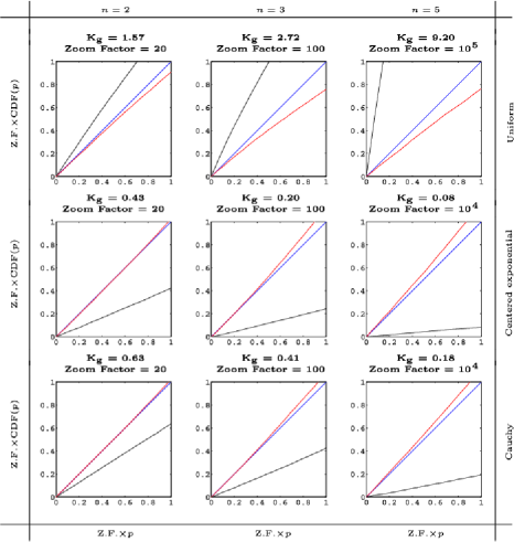
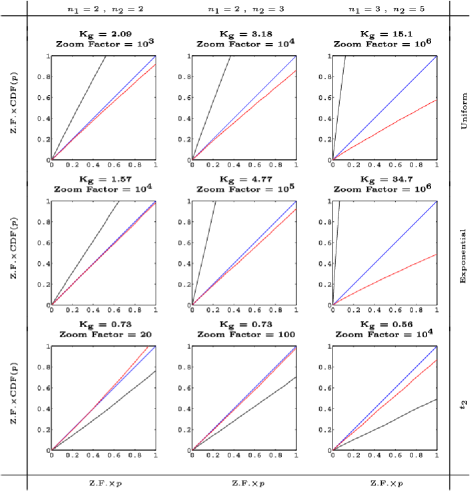
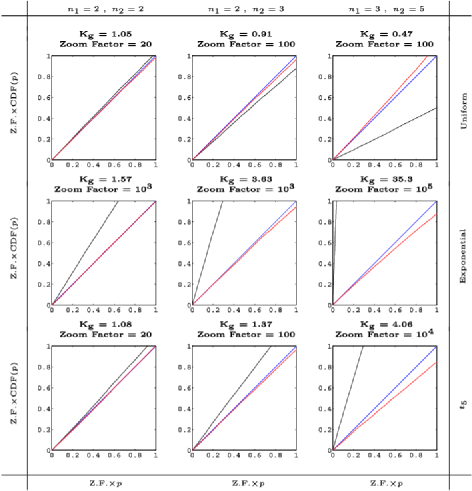
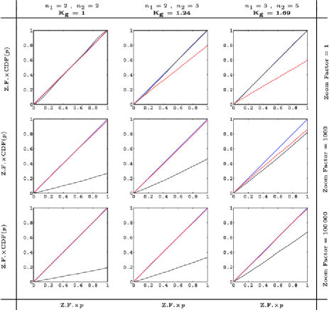
Let $T$ be one of the test statistics considered in the previous sections and $t(u)$ be the distribution tail of $T$ under $H_{0}\colon\ g\sim\operatorname{MVN}(\mathbf{0},\mathbf{1}_{n})$. Next, we choose the sample size, specify the density $g(\mathbf{x})$, and simulate $N$ random vectors $\mathbf{X}\sim g$. For each vector $\mathbf{X}$, we compute $t^{*}=T(\mathbf{X})$, the value of the test statistic $T$, and two $p$-values $p^{R}=t(t^{*})$ and $p^{C}=K_{g}t(t^{*})=K_{g}p^{R}$. Finally, we plot the empirical CDF of $p^{R}$ and $p^{C}$ over the range $I(r)=[0,1/r]$, where the Zoom Factor (Z.F.) parameter $r$ determines the tail region of interest. Here $N=10\,000\times r$ so that $I(r)$ contains approximately $10\,000$ $p$-values (as if they were uniformly distributed) – this is to ensure that the tails of the distribution of the $p$-values $p^{R}$ and $p^{C}$ are equally well approximated by the corresponding CDFs in all the tail regions. The letters “R” and “C” in the notation for the $p$-values stand for “Raw”, that is, computed using $t(u)$, and “Corrected”, that is, computed using $K_{g}t(u)$.

For the i.i.d. case, let $h(x)$, the marginal density of the vector $\mathbf{X}$, be either $\operatorname{Uniform}(-1,1)$, Standard normal, Centered exponential, Cauchy, or $t$-density with $2$ or $5$ degrees of freedom. The constant $K_{g}$ was either evaluated explicitly in Mathematica [11] or computed numerically in MATLAB [12], see Supplementary Materials. Figures 2, 3 and 4 in Appendix B show empirical CDFs for different sample sizes and Zoom Factor $r$ varying between $20$ and $1\,000\,000$. One can see that our approximations are very accurate in the tail regions for all the three test statistics, all sample sizes, and densities $h(x)$ considered in the study. Note also that the convergence speed is better for smaller sample sizes – this is in agreement with the bounds for the absolute error in Lemma 6.1, see Section 6.

Next, we computed $p$-values for the Welch statistic and compared them with the $p$-values obtained using the expression (14) in Corollary 3.2. Here “Raw” $p$-values are obtained using the Welch approximation and the notation is $p^{W}$. According to the plots in the top row of Figure 5, it may seem that the $p$-values $p^{W}$ are uniformly distributed. However, if one “zooms in” to the tail region, see the plots in the middle row of Figure 5, it is clear that the $p$-values obtained using Welch approximation deviate significantly from the theoretical uniform distribution, while the corrected $p$-values $p^{C}$ follow the diagonal line precisely. The advantage of using our tail approximations is fully convincing at Zoom Factor $100\,000$, see the bottom row of Figure 5.

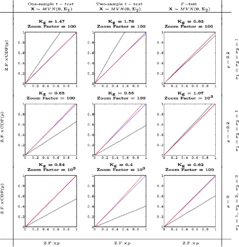
Finally, we made similar plots for even more peculiar scenarios where the data was dependent and non-stationary, see, for example, Figure 6. Our approximations were very accurate in all considered cases.

Appendix A Supplementary theorems and lemmas

This Appendix is split into two parts – the first one introduces the key lemma which is used in Sections 2, 3 and 5, and the second contains useful notes on the regularity constraints (replacing them by simpler criteria that can be used in practice) and shows how to weaken the assumption of continuity of the density $g(\mathbf{x})$.

A.1 Asymptotic behavior of an integral of a continuous function over a shrinking ball

It was shown that the tails of the distribution of the Student one- and two-sample $t$-, Welch, and $F$-statistics are determined by the asymptotic behavior of an integral of some function (different for each of the tests) over a shrinking ball.

Let $G(\mathbf{x})$, $\mathbf{x}\in\mathbb{R}^{k}$ be some real-valued function and consider the asymptotic behavior of

$$F(u)=\mathop{\int\cdots\int}_{\sum x_{i}^{2}<u^{-2}}G(\mathbf{x})\,\mathrm{d}\mathbf{x}$$ (23)

for fixed $k$ and $u\to\infty$.

Lemma A.1

Set $f(u)=\alpha^{-1}F_{m,k}(u^{2})$, where $F_{m,k}(\cdot)$ is the tail of the $F$-distribution with $m\geq 1$ and $k\geq 2$ degrees of freedom, and let $\operatorname{Vol}(B_{k})$ be the volume of the unit $k$-ball $B_{k}$ and $B(x,y)$ be the Beta function. The parameters $\alpha$ and $m$ will be set later. With the above notation we have:

1. [(B)]

2. If $G$ is continuous at zero, then

   $$\frac{F(u)}{f(u)}=K_{G,\alpha}+\mathrm{o}(1)\qquad\mbox{as }u\to\infty,$$ (24)

   where

   $$K_{G,\alpha}=\frac{\alpha kB({m}/{2},{k}/{2})}{2({k}/{m})^{k/2}}\operatorname{Vol}(B_{k})G(\mathbf{0}).$$ (25)

3. If $G$ is differentiable in some neighborhood of zero, then for any $u>0$

   $$\bigl{|}F(u)-K_{G,\alpha}f(u)\bigr{|}\leq\frac{C_{1}}{u^{k+1}}\sup_{{\|\mathbf{x}\|}\leq u^{-1}}\bigl{\|}\nabla G(\mathbf{x})\bigr{\|}+C_{2}\frac{K_{G,\alpha}}{\alpha}\frac{1}{u^{k+2}},$$ (26)

   where

   $$C_{1}=\operatorname{Vol}(B_{k})\quad\mbox{and}\quad C_{2}=\frac{k(k+m)}{m(k+2)}\frac{({k}/{m})^{k/2}}{B({m}/{2},{k}/{2})},$$ (27)

   and $\nabla G(\mathbf{x})$ is a gradient of $G$ evaluated at point $\mathbf{x}$.

4. If $G$ is twice differentiable in some neighborhood of zero, then

   $$u^{k+2}\bigl{(}F(u)-K_{G,\alpha}f(u)\bigr{)}=L_{G,\alpha}+\mathrm{o}(1)\qquad\mbox{as }u\to\infty,$$ (28)

   where

   $$L_{G,\alpha}=C_{1}\frac{\operatorname{tr}(\operatorname{Hess}(G(\mathbf{0})))}{2(k+2)}-C_{2}\frac{K_{G,\alpha}}{\alpha},$$

   $\operatorname{tr}(A)$ is the trace of a square matrix $A$, and $\operatorname{Hess}(G(\mathbf{x}))$ is the Hessian matrix of $G$ evaluated at point $\mathbf{x}$. Constants $C_{1}$ and $C_{2}$ are given by (27).

Proof.

The first statement follows from the asymptotic expansion for the $F$-distribution tail

$$f(u)=\frac{2({k}/{m})^{k/2}}{\alpha kB({m}/{2},{k}/{2})}\biggl{[}\frac{1}{u^{k}}-\frac{k^{2}(k+m)}{2m(k+2)}\frac{1}{u^{k+2}}\biggr{]}+\mathrm{o}\biggl{(}\frac{1}{u^{k+2}}\biggr{)}.$$ (29)

Indeed, changing variables $\mathbf{x}=\mathbf{y}/u$ we write

$$F(u)=\mathop{\int\cdots\int}_{\sum x_{i}^{2}<u^{-2}}G(\mathbf{x})\,\mathrm{d}\mathbf{x}=\frac{1}{u^{k}}\mathop{\int\cdots\int}_{B_{k}}G(\mathbf{y}/u)\,\mathrm{d}\mathbf{y}.$$ (30)

Continuity of $G$ at zero implies uniform convergence of $G(\mathbf{y}/u)$ to $G(\mathbf{0})$ over the ball ${B_{k}}$, and thus

$$F(u)=\operatorname{Vol}(B_{k})G(\mathbf{0})\frac{1}{u^{k}}\bigl{(}1+\mathrm{o}(1)\bigr{)}.$$ (31)

Dividing (31) by (29) we get that the value of $K_{G,\alpha}$ in (24) coincides with (25).

Now assume $G$ is differentiable in some neighborhood of zero and consider the Lagrange form of the Taylor expansion of $G(\mathbf{y}/u)$. The latter and (30) give

$$\bigl{|}F(u)-K_{G,\alpha}f(u)\bigr{|} \leq \frac{1}{u^{k}}\bigl{|}\operatorname{Vol}(B_{k})G(\mathbf{0})-u^{k}K_{G,\alpha}f(u)\bigr{|}$$

$${}+\frac{1}{u^{k+1}}\biggl{|}\mathop{\int\cdots\int}_{B_{k}}\nabla G\bigl{(}\xi(\mathbf{y})\mathbf{y}\bigr{)}\mathbf{y}^{T}\,\mathrm{d}\mathbf{y}\biggr{|},$$

where $0\leq\xi(\mathbf{y})\leq 1/u$. The second summand in the right-hand side of the above inequality is bounded by

$$\frac{1}{u^{k+1}}\operatorname{Vol}(B_{k})\sup_{B_{k}}\bigl{\|}\nabla G(\mathbf{x}/u)\bigr{\|},$$

and the bound for the remaining summand follows from (29), where we note that $f(u)$ is bounded by the two successive partial sums in its alternated series (29) and that the factors before $\operatorname{Vol}(B_{k})G(\mathbf{0})$ in the expression for $K_{G,\alpha}$ and before the square brackets in (29) cancel out. The last step is to use formulas (25) and (27) to express $\operatorname{Vol}(B_{k})G(\mathbf{0})$ in terms of $K_{G,\alpha}$ and $C_{2}$.

We move on to the proof of (28). Taylor expansion for $G(\mathbf{y}/u)$ yields

$$F(u) = \frac{1}{u^{k}}\operatorname{Vol}(B_{k})G(\mathbf{0})$$

$${}+\frac{1}{u^{k+2}}\mathop{\int\cdots\int}_{B_{k}}\frac{\mathbf{y}\operatorname{Hess}(G(\mathbf{0}))\mathbf{y}^{T}}{2}\,\mathrm{d}\mathbf{y}+\mathrm{o}\biggl{(}\frac{1}{u^{k+2}}\biggr{)},$$

where we took into account that the integral of the odd function $\nabla G(\mathbf{0})\mathbf{y}$ over the ball $B_{k}$ is zero. Neglecting odd terms in $\mathbf{y}\operatorname{Hess}(G(\mathbf{0}))\mathbf{y}^{T}$ we have

$$\mathop{\int\cdots\int}_{B_{k}}\mathbf{y}\operatorname{Hess}\bigl{(}G(\mathbf{0})\bigr{)}\mathbf{y}^{T}\,\mathrm{d}\mathbf{y} = \sum\mathop{\int\cdots\int}_{B_{k}}\frac{\partial^{2}G(\mathbf{0})}{\partial^{2}y_{i}}y_{i}^{2}\,\mathrm{d}\mathbf{y}$$

$$= \biggl{(}\sum\frac{\partial^{2}G(\mathbf{0})}{\partial^{2}y_{i}}\biggr{)}\mathop{\int\cdots\int}_{B_{k}}\frac{\sum y_{i}^{2}}{k}\,\mathrm{d}\mathbf{y}$$

$$= \operatorname{Vol}(B_{k})\frac{\operatorname{tr}(\operatorname{Hess}(G(\mathbf{0}))}{k+2},$$

where the last integral was computed using spherical coordinates. Substituting the second order Taylor expansion for $F(u)$ and expression for $f(u)$ in (29) into the left-hand side of (28) we get the constant $L_{G,\alpha}$. ∎

Note that the expression ${\alpha}^{-1}{K_{G,\alpha}}$ does not depend on $\alpha$ and thus the right-hand side of (26) and (28) depends only on the integrand $G$ in (23) and parameters $m$ and $k$.

Corollary A.2

Let $t_{k}(u)$ be the Student $t$-distribution tail with $k$ degrees of freedom. If $G$ is continuous at zero, then

$$\frac{F(u)}{t_{k}(u)}=K_{G,2}+\mathrm{o}(1)\qquad\mbox{as }u\to\infty,$$

where $K_{G,2}$ is given by (25) with $m=1$. Statements (B) and (C) also hold for $f(u)=t_{k}(u)$, provided $m=1$ and $\alpha=2$.

Proof.

Note that $t_{k}(u)=\frac{1}{2}F_{1,k}(u^{2})$ and apply Lemma A.1. ∎

A.2 A note on the regularity constraints and the continuity assumption

The aim of this section is to replace the technical constraints (3), (3) and (17) of Theorems 2.1, 3.1 and 5.1 by simpler criteria, and to weaken the assumption of continuity of the multivariate density $g(\mathbf{x})$ of the data vector $\mathbf{X}$.

The nature of the regularity constraints (3), (3) and (17) becomes clear if one notes that all the proofs share a common part, which is to apply Lemma A.1(A) or Corollary A.2 to the representation for the distribution tail of the test statistic $T$, see (7) and (13), and then to use dominated convergence theorem to show that the corresponding function $G(\mathbf{t})$ is continuous at zero. The only purpose of the regularity constraints is to ensure that the limiting and integration operations are interchangeable, and that the resulting constant $K_{g}$ is finite. Omitting the regularity assumptions (3), (3) and (17) we immediately obtain

Theorem A.3 ((“liminf” analogue of Theorems 2.1, 3.1 and 5.1))

Let $T$ be the Student one- or two-sample $t$-statistic or an $F$-statistic and let $t(u)$ be the distribution tail of $T$ under the null hypothesis $H_{0}\colon\ g\sim\operatorname{MVN}(\mathbf{0},\sigma^{2}\mathbf{1}_{n})$, where $\sigma^{2}>0$ and $\mathbf{1}_{n}$ is the identity matrix. If $g$ is continuous, then

$$\liminf_{u\to\infty}\frac{\mathbf{P}({T>u})}{t(u)}\geq K_{g},$$

where the constant $K_{g}$ is given by (4), (3) and (18) accordingly, though it may not necessarily be finite.

Next, we give the sufficient (but not necessary) conditions for the regularity constraints of Theorems 2.1, 3.1 and 5.1 to hold. One may expect that formulas (5), (11) and (19) hold simply when $g$ is continuous and $K_{g}$ is finite, but proving or disproving this claim is not easy and it remains an open problem.

Lemma A.4

If $g(\mathbf{x})$ is bounded and there exist positive constants $R$, $C$ and $\delta$ such that

$$g(\mathbf{x})\leq\frac{C}{\|\mathbf{x}\|^{n+\delta}}\qquad\mbox{for }\|\mathbf{x}\|>R,$$ (32)

then the assumptions (3), (3) and (17) of Theorems 2.1, 3.1 and 5.1 hold.

Proof.

The integrals in (3), (3) and (17) will be estimated by partitioning the integration domain into several disjoint parts $D_{i}$ and $D^{*}_{j}$ and analyzing the integrals over these sets separately. For non-compact domains $D^{*}_{j}$ the integrand will be estimated from above using the bound (32) and showing that this bound is integrable. The integrability over the compact domains $D_{i}$ follows from the fact that $g(\mathbf{x})$ is bounded. In the notation below let $G(r)$, $G(\omega,r)$ and $G(\mathbf{x},r)$ be the integrands in (3), (3) and (17) accordingly.

Student’s one-sample $t$-statistic: Set $D_{1}=[0,R]$ and $D^{*}_{1}=[R,\infty]$. Since $\mathbf{I}$ and ${\bm{\xi}}$ are orthogonal and taking into account that $\|\mathbf{I}\|=1$ we have $\|r(\mathbf{I}+{\bm{\xi}})\|^{2}=r^{2}(1+\|{\bm{\xi}}\|^{2})\geq r^{2}$, and the bound (32) gives

$$\int_{D_{1}^{*}}G(r)\,\mathrm{d}r<\int_{R}^{\infty}\frac{C}{r^{1+\delta}}\,\mathrm{d}r<\infty.$$

Student’s two-sample $t$-statistic: Setting $D_{1}=[-\uppi/2,\uppi/2]\times[0,R]$ and $D^{*}_{1}=[-\uppi/2,\uppi/2]\times[R,\infty]$ and noting that $\mathbf{I}_{1}$, $\mathbf{I}_{2}$ and ${\bm{\xi}}$ are mutually orthogonal we get

$$\bigl{\|}r\bigl{(}\cos(\omega-\omega_{0})\mathbf{I}_{1}+\sin(\omega-\omega_{0})\mathbf{I}_{2}+{\bm{\xi}}\bigr{)}\bigr{\|}^{2}=r^{2}\bigl{(}1+\|{\bm{\xi}}\|^{2}\bigr{)}\geq r^{2},$$

where we used the fact that $\|\mathbf{I}_{1}\|=\|\mathbf{I}_{2}\|=1$. Now the bound (32) implies

$$\int_{D_{1}^{*}}G(\omega,r)\,\mathrm{d}r<\int_{-\uppi/2}^{\uppi/2}\cos(\omega)^{n-2}\,\mathrm{d}\omega\times\int_{R}^{\infty}\frac{C}{r^{1+\delta}}<\infty.$$

$F$-statistic: Consider the following partition of $\mathbb{R}^{n_{1}+1}\mathchoice{\nobreak\,\colon}{\nobreak\,\colon}{\nobreak\,\colon\;}{\nobreak\,\colon\;}D_{1}=\{(\mathbf{x},r)\mathchoice{\nobreak\,\colon}{\nobreak\,\colon}{\nobreak\,\colon\;}{\nobreak\,\colon\;}\|\mathbf{x}\|\leq R,|r|\leq R\}$, $D_{1}^{*}=\{(\mathbf{x},r)\mathchoice{\nobreak\,\colon}{\nobreak\,\colon}{\nobreak\,\colon\;}{\nobreak\,\colon\;}\|\mathbf{x}\|\leq R,|r|>R\}$, and $D_{2}^{*}=\{(\mathbf{x},r)\mathchoice{\nobreak\,\colon}{\nobreak\,\colon}{\nobreak\,\colon\;}{\nobreak\,\colon\;}\|\mathbf{x}\|>R\}$. Since $\mathbf{I}$ and ${\bm{\xi}}$ are orthogonal and $\|\mathbf{I}\|=1$ we have $\|(\mathbf{x},r\mathbf{I}+s_{1}(\mathbf{x}){\bm{\xi}})\|^{2}=\|\mathbf{x}\|^{2}+r^{2}+s_{1}(\mathbf{x})^{2}\|{\bm{\xi}}\|^{2}\geq\|\mathbf{x}\|^{2}+r^{2}$, and then

$$\mathop{\int\cdots\int}_{D_{1}^{*}}G(\mathbf{x},r)\,\mathrm{d}r\,\mathrm{d}\mathbf{x}<\mathop{\int\cdots\int}_{\|\mathbf{x}\|\leq R}s_{1}(\mathbf{x})^{n_{2}-1}\,\mathrm{d}\mathbf{x}\times\int_{|r|>R}\frac{C}{|r|^{n+\delta}}\,\mathrm{d}r<\infty$$

and

$$\mathop{\int\cdots\int}_{D_{2}^{*}}G(\mathbf{x},r)\,\mathrm{d}r\,\mathrm{d}\mathbf{x} < \mathop{\int\cdots\int}_{\|\mathbf{x}\|>R}\int_{-\infty}^{\infty}\frac{s_{1}(\mathbf{x})^{n_{2}-1}}{(\|\mathbf{x}\|^{2}+r^{2})^{{(n+\delta)}/{2}}}\,\mathrm{d}r\,\mathrm{d}\mathbf{x}$$

$$< \mathop{\int\cdots\int}_{\|\mathbf{x}\|>R}\frac{s_{1}(\mathbf{x})^{n_{2}-1}}{\|\mathbf{x}\|^{n-1+\delta}}\,\mathrm{d}\mathbf{x}\times\int_{-\infty}^{\infty}\frac{1}{(1+r^{2})^{n/2}}\,\mathrm{d}r<\infty,$$

where the multidimensional integral in the last inequality is computed by means of passing to spherical coordinates. ∎

Note that in the i.i.d. case the condition (32) is equivalent to the existence of the $n-1+\delta$ moment of the marginal density $h(x)$. For the Student one-sample $t$-test, however, the criterium of Lemma A.4 is “too strict”, see below.

Definition A.5.

Multivariate density $g(\mathbf{x})$ has the asymptotic monotonicity property if there exists a constant $M$ such that for any $1\leq i\leq n$ and any constants $c_{j}$, $j\neq i$, the function $f(x)=g(c_{1},\ldots,c_{i-1},x,c_{i+1},\ldots,c_{n})$ is monotone on $[M,\infty)$.

Lemma A.6

If $K_{g}$ is finite and $g(\mathbf{x})$ is bounded and has the asymptotic monotonicity property, then the assumption (3) holds.

Proof.

Setting $\varepsilon$ equal to $(2\sqrt{n})^{-1}$ and using asymptotic monotonicity property we get that the integral in (3) is bounded by

$$\int_{0}^{2M\sqrt{n}}r^{n-1}\sup_{\|{\bm{\xi}}\|<{1}/{2\sqrt{n}}}g\bigl{(}r(\mathbf{I}+{\bm{\xi}})\bigr{)}\,\mathrm{d}r+\int_{2M\sqrt{n}}^{\infty}r^{n-1}g\biggl{(}r\frac{\mathbf{I}}{2}\biggr{)}\,\mathrm{d}r<\infty.$$

The first summand is finite owing to the boundness of $g$ and the finiteness of the second summand is equivalent to the finiteness of $K_{g}$. ∎

Asymptotic monotonicity and finiteness of $K_{g}$ are very mild constraints. For the i.i.d. case of the Student one-sample $t$-test, for example, Lemma A.6 implies that the statement of Theorem 2.1 holds for any continuous marginal density $h(\mathbf{x})$ that has monotone tails and such that $K_{g}<\infty$, and the latter assumption is weaker than the assumption of existence of the first moment and holds even for such heavy tailed densities as Cauchy.

Unfortunately there is no asymptotic monotonicity criterium analogue for the case of the Student two-sample $t$- and $F$-statistics, and the constant $K_{g}$ in (3) and (18) may be infinite for some heavy-tailed densities, cf. Bradley [1].

Finally, in the proofs of Theorems 2.1, 3.1 and 5.1 one may have used the “almost everywhere” version of the dominated convergence theorem. For the Student one-sample $t$-statistic the assumption of continuity of $g$ can be replaced by the assumption that $g(\mathbf{x})$ is continuous function of $\mathbf{x}\in\mathbb{R}^{n}$ a.e. on the set of points $\mathbf{x}=r\mathbf{I}$, $r>0$, for the Student two-sample $t$-statistic – on the set of points $\mathbf{x}=r(\cos(\omega-\omega_{0})\mathbf{I}_{1}+\sin(\omega-\omega_{0})\mathbf{I}_{2}+\mathbf{z})$, where $r>0$ and $\omega\in[-\uppi/2,\uppi/2]$, and for the $F$-statistic – on the set of points $\mathbf{x}=\mathbb{R}^{n_{1}}\times r\mathbf{I}$, $r\in\mathbb{R}$. Here a.e. means almost everywhere with respect to the Lebesque measure induced by the measure of the linear space $L$ in (3), (3) and (17).

Appendix B Figures

Figure 2: The eCDF of the $p$-values for the Student one-sample $t$-test. The empirical CDFs of the raw and corrected $p$-values $p^{R}$ and $p^{C}$ are shown in black and red accordingly. The top, middle and bottom rows correspond to the $\operatorname{Uniform}(-1,1)$, Centered exponential and Cauchy densities, and left, middle and right columns correspond to sample sizes $n=2$, $n=3$ and $n=5$. The blue diagonal line is the theoretical uniform distribution. The axes are scaled according to the Zoom Factor (Z.F.) parameter $r$ in the title of the graphs.

Figure 3: The eCDF of the $p$-values for the Student two-sample $t$-test. The empirical CDFs of the raw and corrected $p$-values $p^{R}$ and $p^{C}$ are shown in black and red accordingly. The top, middle and bottom rows correspond to the $\operatorname{Uniform}(-1,1)$, Exponential and $t_{2}$ densities, and left, middle and right columns correspond to sample sizes ($n_{1}=2$, $n_{2}=2$), ($n_{1}=2$, $n_{2}=3$), and ($n_{1}=3$, $n_{2}=5$). The blue diagonal line is the theoretical uniform distribution. The axes are scaled according to the Zoom Factor (Z.F.) parameter $r$ in the title of the graphs.

Figure 4: The eCDF of the $p$-values for the $F$-test (equality of variances). The empirical CDFs of the raw and corrected $p$-values $p^{R}$ and $p^{C}$ are shown in black and red accordingly. The top, middle and bottom rows correspond to the $\operatorname{Uniform}(-1,1)$, Exponential and $t_{5}$ densities, and left, middle and right columns correspond to sample sizes ($n_{1}=2$, $n_{2}=2$), ($n_{1}=2$, $n_{2}=3$), and ($n_{1}=3$, $n_{2}=5$). The blue diagonal line is the theoretical uniform distribution. The axes are scaled according to the Zoom Factor (Z.F.) parameter $r$ in the title of the graphs.

Figure 5: The distribution tails of the $p$-values for the Welch test. The empirical CDFs of the raw (Welch–Satterthwaite) and corrected $p$-values $p^{R}$ and $p^{\mathit{WS}}$ for the Standard Normal density are shown in black and red accordingly. The top, middle and bottom rows correspond to the different values of the Zoom Factor (Z.F.) parameter $r$ shown on the right, and the axes are scaled accordingly. The left, middle and right columns correspond to sample sizes ($n_{1}=2$, $n_{2}=2$), ($n_{1}=2$, $n_{2}=3$), and ($n_{1}=3$, $n_{2}=5$). The blue diagonal line is the theoretical uniform distribution.

Figure 6: The effect of dependency and non-homogeneity of data on $\mathbf{P}({T>u})$ as $u\to\infty$. The empirical CDF of raw (black) and corrected (red) $p$-values. Analogue of Figures 2, 3 and 4 for dependent (top row – positively correlated observations; middle row – negatively correlated observations) and non-homogeneous (bottom row, unequal variances) data. Multivariate normal case with covariance matrices
  $\displaystyle\bm{\Sigma}_{1}=\left(\matrix{\sigma_{1}^{2}&\rho\sigma_{1}\sigma_{2}&0\cr\rho\sigma_{1}\sigma_{2}&\sigma_{2}^{2}&\rho\sigma_{2}\sigma_{3}\cr 0&\rho\sigma_{2}\sigma_{3}&\sigma_{3}^{2}}\right),\qquad\displaystyle\bm{\Sigma}_{2}=\left(\matrix{\sigma_{1}^{2}&\rho\sigma_{1}\sigma_{2}&0&0&0\cr\rho\sigma_{1}\sigma_{2}&\sigma_{2}^{2}&0&0&0\cr 0&0&\sigma_{1}^{2}&\rho\sigma_{1}\sigma_{2}&0\cr 0&0&\rho\sigma_{1}\sigma_{2}&\sigma_{2}^{2}&\rho\sigma_{2}\sigma_{3}\cr 0&0&0&\rho\sigma_{2}\sigma_{3}&\sigma_{3}^{2}}\right)$.