The physics of volume rendering

Abstract

Radiation transfer is an important topic in several physical disciplines, probably most prominently in astrophysics. Computer scientists use radiation transfer, among other things, for the visualisation of complex data sets with direct volume rendering. In this note, I point out the connection between physical radiation transfer and volume rendering, and I describe an implementation of direct volume rendering in the astrophysical radiation transfer code RADMC-3D. I show examples for the use of this module on analytical models and simulation data.

tpeters@physik.uzh.ch

1 Introduction

Radiation transfer plays an important role in several areas of the physical sciences such as atmospheric science, medical physics and astrophysics. Less well known, at least in the physics community, are the various applications of radiation transfer theory in computer graphics. Computer scientists apply physically-inspired radiation transfer not only to create photo-realistic images and animations [phahum, ; foley3, ], but also use it in a non-obvious way for visualisation [preim, ; sabella, ; drebin, ]. Volume rendering is a visualisation technique in which radiation transfer is quintessential and, besides being of immense practical importance, can be very easily understood from physical principles.

In this short note, I introduce the method of direct volume rendering to an audience with a physical background. I provide a dictionary of technical terms used by computer scientists and derive the volume rendering method from the integral form of the well-known radiation transfer equation. I then describe an implementation of direct volume rendering in the freely available astrophysical radiative transfer code RADMC-3D. I conclude with some exemplary applications of this code to analytical models and simulations in astrophysics.

2 The Radiative Transfer Equation and Transfer Functions

The starting point for our considerations is the (one-dimensional) formal radiative transfer equation in integral form [rybickietal79, ; mihalasetal84, ; shu1, ; padmana1, ; peraiah02, ; salby12, ; nelson, ]

$$I_{\nu}(s_{1})=I_{\nu}(s_{0})\exp(-\tau_{\nu}(s_{0},s_{1}))+\int_{s_{0}}^{s_{1}}j_{\nu}(s^{\prime})\exp(-\tau_{\nu}(s^{\prime},s_{1}))\,\mathrm{d}s^{\prime}$$ (1)

Here, $I_{\nu}(s)$ is the intensity of radiation at location $s$, $j_{\nu}(s)$ the emissivity,

$$\tau_{\nu}(s_{0},s_{1})=\int_{s_{0}}^{s_{1}}\alpha_{\nu}(s^{\prime})\,\mathrm{d}s^{\prime}$$ (2)

the optical depth between $s_{0}$ and $s_{1}$, and $\alpha_{\nu}(s)$ is the opacity (or extinction coefficient). All these quantities depend on the frequency $\nu$ as well. The radiation transfer equation (1) is easy to interpret. The radiation that arrives at $s_{1}$ has two contributions. The first term represents the incoming radiation at $s_{0}$, which gets diluted by absorption along the ray from $s_{0}$ to $s_{1}$. The second contribution describes the emission of radiation by the material between $s_{0}$ and $s_{1}$, which gets diluted as well until it arrives at $s_{1}$. Scattering processes are excluded from the formal transfer equation considered here, but can be described by the well-known rendering equation in more advanced treatments [immel, ; kajiya, ; kajiya2, ]. To indicate the omission of scattered radiation, the simple rendering technique employed here is also called emission-absorption model. In the examples considered below, $I_{\nu}(s_{0})$ is set to zero at the domain boundary $s_{0}$, so that (1) only contains the integral term, which physically means that objects are visualised through their own emission and not through their shadowing of some background illumination.

In physics, $j_{\nu}$ and $\alpha_{\nu}$ can describe, e.g., the thermal emission and absorption of dust or of molecular lines. In computer science, however, $j_{\nu}$ and $\alpha_{\nu}$ are designed to visualise volumetric data sets. The basic idea is to send a ray from a camera through the computational domain for each pixel of the image. This procedure is called ray tracing. Along each ray (1) is then solved. Of course, now $j_{\nu}$ and $\alpha_{\nu}$ do not represent any physical processes. Instead, they are defined using transfer functions, and the assignment of a transfer function to a particular grid cell is called classification. For example, we might want to visualise a three-dimensional density field $\rho$. The transfer function $T$ then specifies how much radiation a grid cell (or voxel) in a certain density interval will emit or absorb. To display a density isosurface around $\rho_{0}$, we will choose $T$ such that it is non-zero only in a small interval around $\rho_{0}$. Typical examples for isosurface transfer functions are rectangle functions

$$T(\rho)=\cases{c&for $|\rho-\rho_{0}|\leq\varepsilon$\\ 0&otherwise}$$ (3)

or narrow Gaussians

$$T(\rho)=c\exp\left[-\left(\frac{\rho-\rho_{0}}{\sigma}\right)^{2}\right].$$ (4)

One then defines the emissivity $j(s)=T_{j}(\rho(s))$ and the extinction coefficient $\alpha(s)=T_{\alpha}(\rho(s))$, with the transfer functions for emission and absorption, $T_{j}$ and $T_{\alpha}$, respectively. The choice of a proper transfer function for a given data set is the central problem of direct volume rendering and in general very difficult. In fact, this is a very active research area with important applications in, e.g., medical visualisation [pfister, ].

3 From Intensities to Colours

There are different ways to convert the results of (1) to a colour image. The easiest and least interesting one is to compute (1) only for a single frequency. A colour table can then be used to map each intensity value to a colour. The obvious problem is that integration of the ray over diverse objects in the scene, represented by distinct transfer functions, can lead to the same final intensity value. This method is therefore fundamentally unable to assign a certain colour to a particular object. However, this ability is of course exactly what makes volume rendering so interesting for applications in medical imaging and visualisation.

Another and more difficult option is to assign a colour spectrum to each transfer function. For example, if we describe a colour by its RGB (red, green, blue) values, then we can define transfer functions $T_{\mathrm{R}}$, $T_{\mathrm{G}}$, $T_{\mathrm{B}}$ for each object and solve (1) for the three frequencies $\nu=\mathrm{R},\mathrm{G},\mathrm{B}$. In general, this means that the three emissivities $j_{\mathrm{R}}$, $j_{\mathrm{G}}$, $j_{\mathrm{B}}$ and the three opacities $\alpha_{\mathrm{R}}$, $\alpha_{\mathrm{G}}$, $\alpha_{\mathrm{B}}$ must be specified. However, one generally assumes that all opacities are equal (grey opacities), so that only one opacity $\alpha$ is used. The final intensities $I_{\mathrm{R}}$, $I_{\mathrm{G}}$, $I_{\mathrm{B}}$ can then directly be interpreted as RGB colour values.

As remarked above, finding appropriate transfer functions can be highly non-trivial. We illustrate the problem with the simple example of a density isosurface, modeled with the Gaussian transfer function (4). This isosurface has a certain width around $\rho_{0}$ in physical space (spatial distance between grid cells) and in density space (the parameter $\sigma$ from (4)). The parameters $\sigma$ and $c$ must be chosen such that integration of the intensities $j_{\mathrm{R,G,B}}$ yields the desired colours $I_{\mathrm{R,G,B}}$. However, the spatial width of the isosurface does not have to be the same everywhere. For example, if the isosurface is wider for one ray than for another ray, its colour can be darker or brighter, depending on whether the ray picks up more emission or less. Therefore, an isosurface of varying thickness cannot be visualised with a constant transfer function if all rays should yield the same colour. Methods to compute transfer functions locally based on the variation of the data have been developed to overcome this problem [levoy, ; kindlmann, ]. We here only describe the most basic algorithm, corresponding to the current implementation in RADMC-3D.

4 Raytracing through Volumetric Data

Once the transfer functions for emission and absorption are defined, (1) must be numerically integrated on the grid [hege, ]. Since (1) holds for all points $s_{0}$ and $s_{1}$ along the ray, we can decompose the ray into intervals (not necessarily of equal length) $[s_{k-1},s_{k}]$ and arrive at

$$I_{\nu}(s_{k})=I_{\nu}(s_{k-1})\exp(-\tau_{\nu}(s_{k-1},s_{k}))+\int_{s_{k-1}}^{s_{k}}j_{\nu}(s^{\prime})\exp(-\tau_{\nu}(s^{\prime},s_{k}))\,\mathrm{d}s^{\prime}$$ (5)

for neighbouring grid cells at position $s_{k-1}$ and $s_{k}$. With the abbreviations

$$\theta_{k}=\exp(-\tau_{\nu}(s_{k-1},s_{k}))$$ (6)

and

$$b_{k}=\int_{s_{k-1}}^{s_{k}}j_{\nu}(s^{\prime})\exp(-\tau_{\nu}(s^{\prime},s_{k}))\,\mathrm{d}s^{\prime}$$ (7)

we can write (5) more conveniently as

$$I_{\nu}(s_{k})=I_{\nu}(s_{k-1})\,\theta_{k}+b_{k}.$$ (8)

The quantity $\theta_{k}$ is called transparency of the medium between the grid cells $s_{k-1}$ and $s_{k}$. Note that $\theta_{k}$ can only attain values between $0$ and $1$, corresponding to totally opaque (large $\tau$) and fully transparent (vanishing $\tau$) material, respectively.

Applying (8) recursively from the last grid cell $s_{n}$ back to the first one $s_{0}$, we get

$$I_{\nu}(s_{n}) =I_{\nu}(s_{n-1})\,\theta_{n}+b_{n}$$ (9)

$$=\Big{[}I_{\nu}(s_{n-2})\,\theta_{n-1}+b_{n-1}\Big{]}\,\theta_{n}+b_{n}$$ (10)

$$=I_{\nu}(s_{0})\,\theta_{1}\cdots\theta_{n-1}\,\theta_{n}+b_{1}\,\theta_{2}\cdots\theta_{n-1}\,\theta_{n}+\cdots+b_{n-1}\theta_{n}+b_{n}.$$ (11)

Introducing $b_{0}=I_{\nu}(s_{0})$, which we set to zero, this expression can be written shorter as

$$I_{\nu}(s_{n})=\sum_{k=0}^{n}b_{k}\prod_{j=k+1}^{n}\theta_{j}.$$ (12)

In this form, the sum (12) is evaluated starting from the far side of the domain, and then the summation proceeds towards the camera (back-to-front). However, with the help of an auxiliary variable to store the accumulated transparency, (12) can be integrated in the other direction (front-to-back) [hege, ]. This has the advantage to allow for early ray termination when the transparency gets very small, so that more distant voxels cannot be seen anymore.

To compute (12), the quantities $\theta_{k}$ and $b_{k}$ must be calculated. This requires the numerical integration of the corresponding integrals. Usually, interpolation is used to carry out the quadrature. RADMC-3D supports both first and second order integration methods. The first order scheme assumes that $\alpha_{\nu}$ and $j_{\nu}$ are constant in each cell, so that the integrals can be easily computed analytically. To apply the second order method, $\alpha_{\nu}$ and $j_{\nu}$ are first mapped from the cell centres to the cell corners. These vertex values are computed by averaging over all cells that touch the vertex. When a ray traverses a cell, the entry and exit values of $\alpha_{\nu}$ and $j_{\nu}$ at the position where the ray pierces through the cell faces are determined using bilinear interpolation from the four vertex values of each face. The second order method than integrates the formal radiative transfer equation assuming that $\alpha_{\nu}$ and $j_{\nu}$ vary linearly between the entry and exit values, and in this case an analytical solution is also possible [olson87, ].

RADMC-3D interpolates $\alpha_{\nu}$ and $j_{\nu}$ during the integration of the radiative transfer equation over a single grid cell. This means that the transfer functions are only evaluated once for each grid cell. Computer scientists call this method pre-classification. A better method, named post-classification, instead interpolates the grid variables and applies the transfer functions to the interpolated data. The latter method is known to yield better results and to reduce aliasing artifacts [kaehler, ]. However, since RADMC-3D is an astrophysical radiative transfer code and many grid variables can contribute to the emission and extinction coefficients, a general interpolation of all these variables is prohibitively memory consuming. In practise, aliasing artifacts are visible but not severe with second order integration, but it can be difficult to visualise isosurfaces when the grid variable varies a lot between neighbouring cells.

5 Experiments with Analytical Models

To illustrate the method, we apply it to a very simple analytical model of a prestellar core. We use a cubical volume with a box length of $0.25\,$pc, which we resolve with $100$ grid cells in each direction. We let the number density vary as $n=28$ cm${}^{-3}(r/$pc$)^{-2}$, where $r$ is the radial distance from the centre of the box. We will visualise two isosurfaces. Since the number density follows a power law, we work with the logarithm $\log_{10}n$ instead of the actual density $n$ to get smooth results. We define transfer functions of the form

$$T(n)=\frac{h}{w}\exp\left[-0.5\left(\frac{\log_{10}n-\log_{10}n_{0}}{\sigma}\right)^{2}\right].$$ (13)

The normalisation constant $w=2.5\times 10^{16}\,$cm is of the order of the size of a grid cell and chosen such that the integration over the Gaussian results in the desired colour. Experimentation is required to find suitable values for $w$. The amplitude $h$ is different for the four transfer functions $j_{\mathrm{R}}$, $j_{\mathrm{G}}$, $j_{\mathrm{B}}$ and $\alpha$. For the first isosurface, we set $\log_{10}n_{0}=3.5$, $\sigma=0.05$ and $(h_{\mathrm{R}},h_{\mathrm{G}},h_{\mathrm{B}},h_{\alpha})=(0.4,0.4,0.8,0.001)$ (purple with almost no absorption), for the second isosurface we pick $\log_{10}n_{0}=4.0$, $\sigma=0.1$ and $(h_{\mathrm{R}},h_{\mathrm{G}},h_{\mathrm{B}},h_{\alpha})=(0.89,0.47,0.06,0.001)$ (ochre).

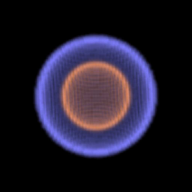
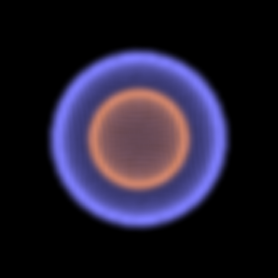
The first panel of Fig. 1 shows the resulting image using first order integration. We see the two spherical isosurfaces, which correspond to the different densities, with their respective colours. Since the rays pick up more contributions from the transfer functions when they hit the isosurface tangentially, the boundaries of the spheres are much brighter than their interiors. This is analogous to, e.g., giant H ii  region bubbles in the interstellar medium, where the boundaries are visible by exactly the same mechanism. We also see pronounced grid artifacts in the image. The middle panel of Fig. 1 displays the result of the second order integration. Here, these artifacts are much reduced. The third panel illustrates the effect of setting $\alpha=0.1$ for the inner isosurface, which makes this isosurface more opaque.

Figure 1: Isosurfaces for an analytical model. The panels show, from left to right, the images generated using first order integration, second order integration, and second order integration with an enhanced opacity for the inner isosurface.

6 Visualisation of Simulation Data

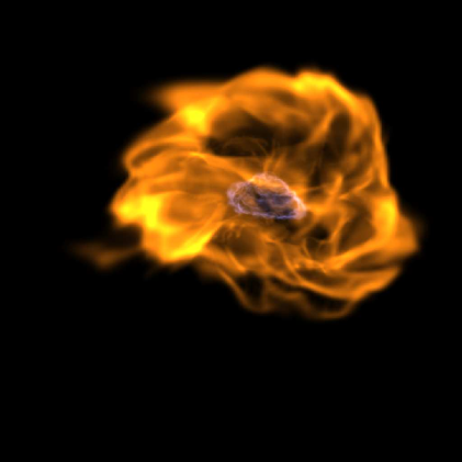
Apart from its use to create analytical models, RADMC-3D can also be employed to post-process simulation data. We demonstrate this with two examples. The left panel of Fig. 2 shows density isosurfaces of a minihalo taken from a simulation of primordial star formation [petersetal12c, ]. Such minihalos typically collapse monolithically, creating an onion-like density structure very similar to the one in our analytical model. We have used the same colours as in the previous section, but have adapted the normalisation constants for this particular situation. This time, the higher densities are shown in purple and the lower ones in ochre. One can nicely see how the isosurfaces are deformed by turbulent motions during the collapse of the halo.

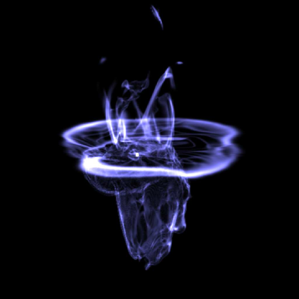
The right panel of Fig. 2 features a density isosurface of an ionisation-driven molecular outflow, taken from a collapse simulation of massive star formation including ionisation feedback [petersetal10a, ]. The isosurface shows both the disk in which the star forms as well as the outflow driven perpendicular to it. A fourth frequency channel was used to display the star that drives the outflow, simply using a rectangle function with a small radius around the star and drawing the resulting emission in the foreground of the image. One can see that the purple colour becomes white were rays intersect the isosurface several times or where the isosurface is thicker than elsewhere. Again, this is because we are assuming a constant thickness of the isosurface, which is clearly not the case. On the lower part of the image, some dark aliasing artifacts can be seen that are likely due to our use of pre-classification.

Apart from the generation of nice images, this volume rendering module for RADMC-3D is also useful for diagnostic purposes because the transfer functions can be made arbitrarily complex. For example, one might want to see an isosurface of density for all gas moving with a certain velocity, coloured according to the temperature of the gas. Generating such a visualisation might be hard or even impossible with standard visualisation tools.

The integration of the radiative transfer equation for arbitrary transfer functions can also be used to measure physical quantities. For example, using the opacities $\alpha_{M}=\rho$, $\alpha_{P}=\rho\,v$ and $\alpha_{E}=0.5\,\rho\,v^{2}$ with the gas density $\rho$ and velocity $v$ we can compute the mass $M$, momentum $P$ and kinetic energy $E$ of the outflow by looking at the optical depth instead of the intensity. These exact values can then be compared with figures derived using observational techniques like synthetic CO line measurements [petersetal12b, ]. This method is particularly useful when the outflows are misaligned with the grid axes, so that a direct measurement from the simulation data is not straightforward.

Figure 2: (left) Density isosurfaces of a primordial minihalo [petersetal12c, ]. One can see the onion-like structure of the gas density. (right) Density isosurface of an ionisation-driven molecular outflow [petersetal10a, ]. The star that drives the outflow by its radiation feedback is shown in the centre of the image.

7 Conclusions

I have pointed out an interesting connection between the physics of radiation transfer and the visualisation technique of direct volume rendering. I have explained how the terminology used by computer scientists fits into the physical framework and described an implementation of direct volume rendering in the astrophysical radiative transfer code RADMC-3D. I believe that the connection between computer graphics and radiation transfer is an attractive topic for students and teachers not only of astrophysics, and that it can also help to better understand analytical models and numerical simulations.

References

- [1] M. Pharr and G. Humphreys. Physically Based Rendering: From Theory to Implementation. Morgan Kaufmann, second edition, 2010.
- [2] J. F. Hughes, A. van Dam, M. McGuire, D. Sklar, J. D. Foley, S. K. Feiner, and K. Akeley. Computer Graphics: Principles and Practice. Addison-Wesley, third edition, 2013.
- [3] B. Preim and D. Bartz. Visualization in Medicine: Theory, Algorithms, and Applications. Morgan Kaufmann, 2007.
- [4] P. Sabella. A rendering algorithm for visualizing 3d scalar fields. SIGGRAPH Comput. Graph., 22(4):51–58, 1988.
- [5] R. A. Drebin, L. Carpenter, and P. Hanrahan. Volume rendering. SIGGRAPH Comput. Graph., 22(4):65–74, 1988.
- [6] G. B. Rybicki and A. P. Lightman. Radiative processes in astrophysics. John Wiley & Sons, Inc., 1979.
- [7] D. Mihalas and B. W. Mihalas. Foundations of Radiation Hydrodynamics. Oxford University Press, 1984.
- [8] F. H. Shu. The physics of astrophysics, volume I: Radiation. University Science Books, 1991.
- [9] T. Padmanabhan. Theoretical Astrophysics, volume I: Astrophysical Processes. Cambridge University Press, 2000.
- [10] A. Peraiah. An Introduction to Radiative Transfer. Cambridge University Press, 2002.
- [11] M. L. Salby. Physics of the Atmosphere and Climate. Cambridge University Press, 2012.
- [12] N. Max. Optical models for direct volume rendering. IEEE Transactions on Visualization and Computer Graphics, 1(2):99–108, 1995.
- [13] D. S. Immel, M. F. Cohen, and D. P. Greenberg. A radiosity method for non-diffuse environments. SIGGRAPH Comput. Graph., 20(4):133–142, August 1986.
- [14] J. T. Kajiya. The rendering equation. SIGGRAPH Comput. Graph., 20(4):143–150, 1986.
- [15] J. T. Kajiya and B. P. Von Herzen. Ray tracing volume densities. SIGGRAPH Comput. Graph., 18(3):165–174, January 1984.
- [16] W. E. Lorensen and H. E. Cline. Marching cubes: A high resolution 3d surface construction algorithm. SIGGRAPH Comput. Graph., 21(4):163–169, 1987.
- [17] H. Pfister, B. Lorensen, C. Bajaj, W. Kindlmann, G.and Schroeder, L. S. Avila, K. Martin, R. Machiraju, and J. Lee. The transfer function bake-off. IEEE Comput. Graph. Appl., 21(3):16–22, 2001.
- [18] M. Levoy. Display of surfaces from volume data. IEEE Comput. Graph. Appl., 8(3):29–37, 1988.
- [19] G. Kindlmann and J. W. Durkin. Semi-automatic generation of transfer functions for direct volume rendering. In Proceedings of the 1998 IEEE Symposium on Volume Visualization, VVS ’98, pages 79–86, New York, NY, USA, 1998. ACM.
- [20] H.-C. Hege, T. Höllerer, and D. Stalling. Volume rendering - mathematicals models and algorithmic aspects. Technical Report TR-93-07, ZIB, 1993.
- [21] G. L. Olson and P. B. Kunasz. Short characteristic solution of the non-LTE transfer problem by operator perturbation. I. The one-dimensional planar slab. J. Quant. Spectrosc. Radiat. Transfer, 38(5):325–336, 1987.
- [22] R. Kähler. Accelerated Volume Rendering on Structured Adapative Meshes. Dissertation, FU Berlin, 2005.
- [23] T. Peters, D. R. G. Schleicher, R. S. Klessen, R. Banerjee, C. Federrath, R. J. Smith, and S. Sur. The impact of thermodynamics on gravitational collapse: filament formation and magnetic field amplification. The Astrophysical Journal, 760:L28, 2012.
- [24] T. Peters, R. Banerjee, R. S. Klessen, M.-M. Mac Low, R. Galván-Madrid, and E. R. Keto. H II regions: Witnesses to massive star formation. The Astrophysical Journal, 711:1017–1028, 2010.
- [25] T. Peters, P. D. Klaassen, M.-M. Mac Low, R. S. Klessen, and R. Banerjee. Are molecular outflows around high-mass stars driven by ionization feedback? The Astrophysical Journal, 760:91, 2012.