Numerical analysis of the vertex models for simulating grain boundary networks

Abstract

Polycrystalline materials undergoing coarsening can be represented as evolving networks of grain boundaries, whose statistical characteristics describe macroscopic properties. The formation of various statistical distributions is extremely complex and is strongly influenced by topological changes in the network. This work is an attempt to elucidate the role of these changes by conducting a thorough numerical investigation of one of the simplest types of grain growth simulation models, the vertex model. While having obvious limitations in terms of its ability to represent realistic systems, the vertex model enables full control over topological transitions and retains essential geometric features of the network.

We formulate a self-consistent vertex model and investigate the role of microscopic parameters on mesoscale network behavior. This study sheds light on several important questions, such as how statistics are affected by the choice of temporal and spatial resolution and rules governing topological changes. Statistical analysis of the data produced by the simulation is performed for both isotropic and anisotropic grain boundary energies.

siapxxxxxxxx–x

1 Introduction

Polycrystalline materials such as metals and ceramics are comprised of single crystallites, called grains, separated by their boundaries, called grain boundaries. The orientations, shapes, and arrangements of the grains have a direct relationship to macroscopic materials properties. For example, the presence of grain boundaries decreases thermal and electrical conductivity that affects the performance of chips in microprocessors. Grain boundaries disrupt motion of dislocations through a material, so reducing crystallite size is a common way to improve strength and fracture toughness in structures, as described by the Hall-Petch relationship [1].

The grain and grain boundary configuration, or the microstructure of a material, is determined by a variety of factors, such as history of deformation, phase transitions, heat treatment, etc. In this paper, we are primarily interested in the process of microstructural relaxation known as coarsening. Evolution of the grain boundary network during coarsening is driven by the tendency of the system to reduce its total grain boundary surface energy spatially constrained that results in growth of some grains at the expense of others, as well as in disappearance and nucleation of both small grains and grain boundaries. In this process the average grain size increases, while the total surface area of the grain boundaries decreases. As it evolves, the grain boundary network begins to exhibit stable, self-similar statistical features that can be described by a finite number of time-dependent parameters. These parameters, in turn, can be used as continuum descriptors of the network.

One of the principal goals of mathematical modeling of polycrystalline materials is to understand how the statistics of an evolving grain boundary network depend on the set of laws that govern the dynamics of the network at the microscopic scale. Here the laws in question describe the motion of grain boundaries and their junctions, as well as the criteria for nucleation and disappearance of grains and grain boundaries. Although these laws have been known for quite some time, their precise role in the development of macroscopic properties of the network is still not fully clear. A possible way to establish a connection between the statistical features of the network and the evolution of individual grain boundaries involves numerical experimentation using large-scale simulation models. As a starting point, it is therefore desirable to consider models that are as simple and as computationally inexpensive as possible, yet preserve the essential characteristics of the original grain boundary network. In what follows we concentrate on two-dimensional polycrystalline materials that can be thought of as, e.g., cross-sections of systems of columnar grains in aluminum films [2].

Since the motion of grain boundaries is controlled by surface energy, it is normally modeled within the framework of curvature-driven growth. Under certain assumptions on relative mobilities of the boundaries and their junctions, it is possible to assume that the boundaries remain straight during the evolution so that the changes within the network can be described solely in terms of motion of the junctions, or vertices, of the graph formed by the boundaries. Note that for isotropic surface energies, only the junctions between three grain boundaries, as opposed to four or five, for instance, are stable. Vertex models that discount grain boundary motion in favor of triple junction motion are used extensively, both due to their computational simplicity in handling extremely large scale networks, and for the purpose of isolating properties local to triple junctions, for example triple junction drag. Following the pioneering works of Fullman [3] in the 50’s and Frost et al. in the 80’s [4], a number of extensions of the original algorithm have been proposed [5]-[11]. The vertex models have been able to reproduce many characteristic features of the cellular pattern growth in foams [12, 13] and to some extent in polycrystals [14]. They have high flexibility, which motivates continued interest in their use despite the existence of more sophisticated numerical codes. The vertex model approach has been recently applied to the recrystallization of ferritic stainless steels [15] and, more generally, to grain growth [14], [16]. It has also been extensively used to validate topological theories of grain growth and Zener pinning [17], [18]. A comprehensive review of the relevant literature can be found in the chapter dedicated to vertex models in [19].

In this paper we develop a numerical algorithm for a version of a simple vertex model originally proposed by Kawasaki in [5]. Our main aims are to derive the set of rules for topological transitions within the network that are consistent with continuous evolution of vertices as well as to control the stability and accuracy of the code. This is done in order to eliminate numerical issues from the investigation of the role that various model parameters play in the development of statistical features. We demonstrate that, although simple, our model results in rich statistics that are reminiscent of what is observed in experiments and more sophisticated simulations. We emphasize, however, that our main motivation is not to replicate or explain experimental observations, but to ensure the correct characterization of the complexity of network behavior. In a subsequent publication we will investigate the formation of statistics using numerical experimentation with the vertex model developed here. This investigation will expand on our prior studies of a one-dimensional model [20, 21, 22].

The paper is organized as follows. In Section 2, we start by formulating a general energy-based model of an evolving grain boundary network. We formally demonstrate that this model reduces to a vertex model by assuming that the mobility of the vertices is much lower than the mobility of grain boundaries evolving via curvature-driven motion. Next, in Sections 3 and 4 we use semi-rigorous analysis of vertex dynamics to derive the set of neighbor switching rules as well as estimates of vertex collision times. Stability analysis of the explicit numerical scheme used in the main algorithm is given in Section 5. The full description of the algorithm appears in Section 6, followed by the numerical results in Section 8. We begin this section by testing the numerical procedure for accuracy and convergence. The procedure is then employed to simulate coarsening of grain boundary networks containing a large number of grains. The geometry of configurations that develop in these simulations is described using the standard statistical measures for characterizing grain growth. These include distributions of relative areas of grains, dihedral angle, number of sides, among others. We are able to confirm spatiotemporal stability of the distributions that emerge in a network evolving via our numerical algorithm. We find that the distributions are essentially independent of the level of numerical resolution as the network appears to pass through the sequence of similar states, possibly at different rates. While mesoscopically the model is insensitive to various modifications, including the rules governing topological changes, the microscopic features of the network tend to differ with the scenario.

2 Vertex model formalism

Let us define the configuration and establish the law of evolution for our network. Suppose given a rectangular domain $R\subset\mathbb{R}^{2}$ that contains a set $\mathbf{\Gamma}$ of $K>0$ smooth curves $\Gamma_{k}:=\left\{\mathbf{x}=\boldsymbol{\xi}_{k}(s),\ 0\leq s\leq L_{k}\right\},\ k=1,\ldots,K,$ that we will call grain boundaries, with $L_{k}>0$ the length of the $k$-th boundary. On a grain boundary curve $\Gamma_{k}$, one can define an orthogonal frame $\left\{\mathbf{b}_{k},\mathbf{n}_{k}\right\}$, where

$$\mathbf{b}_{k}=\frac{d\boldsymbol{\xi}_{k}}{ds}/\left|\frac{d\boldsymbol{\xi}_{k}}{ds}\right|\ \textrm{and}\ \mathbf{n}_{k}=\frac{d\mathbf{b}_{k}}{ds}/\left|\frac{d\mathbf{b}_{k}}{ds}\right|$$

Assuming periodic boundary conditions on $\partial R,$ all grain boundaries can terminate only at junctions with other boundaries. We denote the set of all junctions in $R$ by $\mathbf{X}:=\left\{\mathbf{x}_{1}^{n_{1}},\mathbf{x}_{2}^{n_{2}},\ldots,\mathbf{x}_{M}^{n_{M}}\right\},$ where the number of junctions, $M\in\mathbb{N}$. Here an $n-$tuple junction $\mathbf{x}_{m}^{n}$ is a terminal point of $n$ grain boundaries $\Gamma_{j_{1}}$, $\Gamma_{j_{2}},\ldots,\Gamma_{j_{n}}$, for some $j_{1},\ j_{2},\ldots,j_{n}\in\left\{1,\ldots,K\right\}$. In the simplest and most commonly studied type of a grain boundary network, the numbers $n_{1}=n_{2}=\ldots=n_{M}=3,$ i.e., all elements of $\mathbf{X}$ are triple junctions.

The grain boundaries contained in $\mathbf{\Gamma}$ subdivide the domain $R$ into $N$ disjoint regions $\left\{\Sigma_{1},\ldots,\Sigma_{N}\right\}=:\mathbf{\Sigma}$, called grains. With each grain $\Sigma_{l}\in\mathbf{\Sigma}$, $l=1,\ldots,N,$ we associate an orientation $\alpha_{l}\in[0,2\pi)$ and the set of grain boundaries $\partial\Sigma_{l}=\left\{\Gamma_{k_{1}},\ldots,\Gamma_{k_{l}}\right\}$ that enclose $\Sigma_{l}.$ Likewise, for each grain boundary $\Gamma_{k},$ $k=1,\ldots,K,$ there are exactly two grains $\Sigma_{l_{1}(k)}$ and $\Sigma_{l_{2}(k)}$ that are separated by $\Gamma_{k}.$

The grain misorientation parameter $\Delta\alpha_{k}$ is defined as $\Delta\alpha_{k}:=\alpha_{l_{2}(k)}-\alpha_{l_{1}(k)},$ where $k=1,\ldots,K.$ The grain boundary energy, $\gamma_{k},$ will be assumed to depend only on misorientation, i.e. $\gamma_{k}=\gamma\left(\Delta\alpha_{k}\right)$ for every $k=1,\ldots,K$ and some given function $\gamma:\mathbb{R}\to\mathbb{R}$. The function $\gamma$ is even and periodic with a period that depends on the symmetries of crystalline lattices of neighboring grains.

We will assume that the grain boundary network evolves in time via simultaneous motion of both the grain boundaries and their junctions. In the course of this motion, some grains grow and some shrink. Once the length of a grain boundary or the area of a grain decreases to zero, we will say that a component of the network has disappeared as a result of a topological transition. In order to describe the evolution of the grain boundary network, both the laws of continuous motion of the boundaries and junctions as well as the rules governing the topological transitions must be specified. From now on we will assume that the sets $\mathbf{\Gamma},\mathbf{X}$ and $\mathbf{\Sigma}$ depend on time $t>0.$

We begin the discussion of the network dynamics by considering a period of time $[t_{0},t_{0}+T]$ during which no topological transitions occur. Introduce the total energy of the network

$$E(t)=\sum_{k=1}^{K}\int_{0}^{L_{k}}\gamma\left(\Delta\alpha_{k}\right)|\mathbf{l}_{k}(s,t)|ds,\quad\mathbf{l}_{k}=\frac{d\boldsymbol{\xi}_{k}}{ds},$$

where all curves at $t_{0}$ are assumed to be parametrized with respect to their arc-length and $L_{k}$ is the length of $\Gamma_{k}$ at the time $t_{0}$. Denoting $\gamma_{k}=\gamma\left(\Delta\alpha_{k}\right)$, we obtain

$$\frac{d}{dt}E(t)=\sum_{k=1}^{K}\int_{0}^{L_{k}}\gamma_{k}\frac{\mathbf{l}_{k}}{|\mathbf{l}_{k}|}\cdot\frac{\partial\mathbf{l}_{k}}{\partial t}ds=\sum_{k=1}^{K}\int_{0}^{L_{k}}\gamma_{k}\mathbf{b}_{k}\cdot\frac{\partial\mathbf{v}_{k}}{\partial s}ds=\sum_{k=1}^{K}\int_{0}^{L_{k}}\mathbf{T}_{k}\cdot\frac{\partial\mathbf{v}_{k}}{\partial s}ds$$

where $\mathbf{T}_{k}=\gamma_{k}\mathbf{b}_{k}$ denotes the capillary force, also called the line tension. Further, $\mathbf{v}_{k}(s,t)$ denotes the velocity of the material point $s$ on the curve $\Gamma_{k}$ at the time $t$ so that

$${\frac{\partial\mathbf{l}_{k}}{\partial t}=\frac{\partial}{\partial t}\left(\frac{\partial\boldsymbol{\xi}_{k}}{\partial s}\right)=\frac{\partial}{\partial s}\left(\frac{\partial\boldsymbol{\xi}_{k}}{\partial t}\right)=\frac{\partial\mathbf{v}_{k}}{\partial s}}.$$

Integrating by parts and using the Frenet formula $\displaystyle{\frac{\partial\mathbf{b}_{k}}{\partial s}=\kappa_{k}|\mathbf{l}_{k}|\mathbf{n}_{k}}$ we obtain

(1) $$\frac{d}{dt}E(t)=-\sum_{k=1}^{K}\int_{0}^{L_{k}}\kappa_{k}V_{k}|\mathbf{l}_{k}|ds-\sum_{m=1}^{M}\mathbf{v}_{m}\cdot\sum_{l=1}^{n_{m}}\mathbf{T}_{m,l},$$

where $\mathbf{T}_{m,l}$ is the capillary force along the grain boundary $\Gamma_{j_{l}}$ that ends at the triple junction $\mathbf{x}_{m}^{n_{m}}.$ Further, $\kappa_{k}$ and $V_{k}=\mathbf{v}_{k}\cdot\mathbf{n}_{k}$ are the curvature and the normal velocity of $\Gamma_{k},$ respectively.

The simplest framework to enforce energy dissipation is to assume that the grain boundaries and their junctions follow a version of gradient flow dynamics. Then the normal velocity of the boundary $\Gamma_{k}$ and the velocity $\mathbf{v}_{m}:=\frac{d}{dt}\mathbf{x}_{m}^{n_{m}}$ of the triple junction $\mathbf{x}_{m}^{n_{m}}$ can be written as

(2) $$V_{k}=\mu_{k}\kappa_{k}$$

and

(3) $$\mathbf{v}_{m}=\lambda_{m}\sum^{n_{m}}_{l=1}{\mathbf{T}_{m,l}},$$

respectively. Here $\mu_{k}>0$ is the mobility of $\Gamma_{k}$ and $\lambda_{m}>0$ is the mobility of $\mathbf{x}_{m}^{n_{m}}$. Then, using (1), we have

(4) $$\frac{d}{dt}E(t)=-\sum_{k=1}^{K}\mu_{k}\int_{0}^{L_{k}}\kappa_{k}^{2}|\mathbf{l}_{k}|ds-\sum_{m=1}^{M}\lambda_{m}{\left|\sum^{n_{m}}_{l=1}{\mathbf{T}_{m,l}}\right|^{2}}\leq 0$$

(2) and (3) are known as the Mullins Equation [23, 24] and a variation of the Herring Condition [25] respectively, cf. also [26].

When the grain boundary mobility is much higher than that of triple junctions, the grain boundaries $\Gamma_{k}$ are essentially straight lines throughout the evolution. The precise asymptotic reduction, which we will not treat here, requires boundary layer analysis near the junctions [27]. Hence the dynamics of the grain boundary network is completely determined by the motion of the triple junctions via the law (3) which relates the velocity of a triple junction to the sum of capillary forces acting on it. This reduced model is known as a vertex model in the literature and is a subject of study in this work.

In what follows, we will set $\lambda_{m}=1$ for all $m=1,\ldots,M$ and, unless noted otherwise, assume that the grain boundary energy is only weakly anisotropic, i.e., $\gamma(\Delta\alpha)=1+\varepsilon f(\Delta\alpha),$ where $\varepsilon>0$ is small. As we will soon see, this assumption ensures that all grain boundary junctions are, in fact, triple junctions and $n_{m}=3$ for all $m=1,\ldots,M$. Thus we can refer to triple junctions simply as $\mathbf{x}_{m},\ m=1,\ldots,M$ by dropping the superscript index $n_{m}$.

Suppose now that $\mathbf{x}_{m_{1}},\ \mathbf{x}_{m_{2}},\ \mathrm{and}\ \mathbf{x}_{m_{3}}$ denote three vertices connected to a vertex $\mathbf{x}_{m}$ for every $m=1,\ldots,M$. Let $\gamma_{mm_{1}},\ \gamma_{mm_{2}},\ \mathrm{and}\ \gamma_{mm_{3}}$ be the grain boundary energy of the straight edges connecting $\mathbf{x}_{m}$ with $\mathbf{x}_{m_{1}},\ \mathbf{x}_{m_{2}},\ \mathrm{and}\ \mathbf{x}_{m_{3}},$ respectively. Then the law of the vertex motion (3) takes the form

(5) $$\dot{\mathbf{x}}_{m}=\sum_{i=1}^{3}\gamma_{mm_{i}}\frac{\mathbf{x}_{m_{i}}-\mathbf{x}_{m}}{\left\|\mathbf{x}_{m_{i}}-\mathbf{x}_{m}\right\|},\ m=1,\ldots,M.$$

In order to fully describe the evolution of the grain boundary network, it is still necessary to understand what happens during topological transitions that alter the structure of the network. This is the subject of the next section.

3 Topological transitions

As discussed earlier, a topological transition occurs when an element of a grain boundary network disappears. This can happen when the length of a single edge, or area of a single grain decreases to zero. In this section, we formulate a set of rules that govern topological transitions. Our approach aims to improve on existing literature by emphasizing the consistency between continuous evolution of the network and discrete transitions.

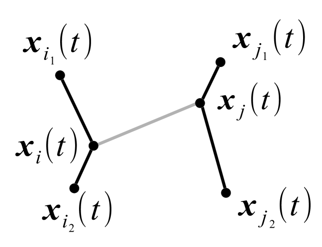
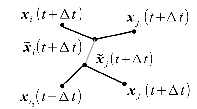
Suppose first that an edge connecting two vertices $\mathbf{x}_{i}$ and $\mathbf{x}_{j}$ disappears at some time $t_{0}>0$. We will then say that $\mathbf{x}_{i}$ and $\mathbf{x}_{j}$ collide at the time $t_{0}$ forming a quadruple junction. When the grain boundary energy is weakly anisotropic, this junction is unstable in the following sense: it is possible to split the quadruple junction into two new triple junctions $\mathbf{\tilde{x}}_{i}$ and $\mathbf{\tilde{x}}_{j}$ connected by an infinitesimally short edge that will grow. Clearly, as indicated in Fig. 1, the direction in which the splitting occurs is not the same as the direction of the original collision. We will refer to this event as a neighbor switching.

Fig. 1: Neighbor switching.

Next, we will use (5) to determine the orientation of the edge that forms as a result of neighbor switching. Fix a sufficiently small $\Delta t>0$, then

(6) $$\dot{\mathbf{x}}_{i} =\gamma_{ii_{1}}\,\frac{\mathbf{x}_{i_{1}}-\mathbf{x}_{i}}{\|\mathbf{x}_{i_{1}}-\mathbf{x}_{i}\|}+\gamma_{ii_{2}}\,\frac{\mathbf{x}_{i_{2}}-\mathbf{x}_{i}}{\|\mathbf{x}_{i_{2}}-\mathbf{x}_{i}\|}+\gamma_{ij}\,\frac{\mathbf{x}_{j}-\mathbf{x}_{i}}{\|\mathbf{x}_{j}-\mathbf{x}_{i}\|},$$

(7) $$\dot{\mathbf{x}}_{j} =\gamma_{jj_{1}}\,\frac{\mathbf{x}_{j_{1}}-\mathbf{x}_{j}}{\|\mathbf{x}_{j_{1}}-\mathbf{x}_{j}\|}+\gamma_{jj_{2}}\,\frac{\mathbf{x}_{j_{2}}-\mathbf{x}_{j}}{\|\mathbf{x}_{j_{2}}-\mathbf{x}_{j}\|}+\gamma_{ij}\,\frac{\mathbf{x}_{i}-\mathbf{x}_{j}}{\|\mathbf{x}_{i}-\mathbf{x}_{j}\|},$$

when $t\in(t_{0}-\Delta t,t_{0}).$ Note that the first two terms in both equations are continuous functions of $t$ on $[t_{0}-\Delta t,t_{0}]$ if we assume that $\mathbf{x}_{i}$ and $\mathbf{x}_{j}$ are continuous on $[t_{0}-\Delta t,t_{0}].$ Subtracting (6) from (7) we have

(8) $$({\mathbf{x}}_{j}-{\mathbf{x}}_{i})\dot{\,}=\mathbf{p_{-}}(t)-2\gamma_{ij}\,\frac{\mathbf{x}_{j}-\mathbf{x}_{i}}{\|\mathbf{x}_{j}-\mathbf{x}_{i}\|},$$

where

(9) $${\bf p}_{-}=\gamma_{jj_{1}}\,\frac{\mathbf{x}_{j_{1}}-\mathbf{x}_{j}}{\|\mathbf{x}_{j_{1}}-\mathbf{x}_{j}\|}+\gamma_{jj_{2}}\,\frac{\mathbf{x}_{j_{2}}-\mathbf{x}_{j}}{\|\mathbf{x}_{j_{2}}-\mathbf{x}_{j}\|}-\gamma_{ii_{1}}\,\frac{\mathbf{x}_{i_{1}}-\mathbf{x}_{i}}{\|\mathbf{x}_{i_{1}}-\mathbf{x}_{i}\|}-\gamma_{ii_{2}}\,\frac{\mathbf{x}_{i_{2}}-\mathbf{x}_{i}}{\|\mathbf{x}_{i_{2}}-\mathbf{x}_{i}\|}$$

satisfies $\mathbf{p_{-}}\in C([t_{0}-\Delta t,t_{0}]).$ Let $\mathbf{x}_{j}-\mathbf{x}_{i}=\rho\mathbf{n}$, where $\rho=\left\|\mathbf{x}_{j}-\mathbf{x}_{i}\right\|$ and $\mathbf{n}=(\cos{\theta},\sin{\theta})$ and set $\boldsymbol{\tau}=(-\sin{\theta},\cos{\theta})$. Rewriting (8), we have

(10) $$\dot{\rho}\mathbf{n}+\rho\dot{\theta}\boldsymbol{\tau}=\mathbf{p_{-}}-2\gamma_{ij}\mathbf{n},$$

or by orthogonal decomposition,

(11a) $$\dot{\rho}=\mathbf{p_{-}}\cdot\mathbf{n}-2\,\gamma_{ij},$$

(11b) $$\dot{\theta}=\frac{\mathbf{p_{-}}\cdot\boldsymbol{\tau}}{\rho}.$$

In Appendix 1, we use (11b) to show that

$$\lim_{t\to t_{0}^{-}}\mathbf{p_{-}}\cdot\boldsymbol{\tau}=0,$$

since $\lim_{t\to t_{0}^{-}}\rho=0.$ Thus $\mathbf{n}_{-}:=\lim_{t\to t_{0}^{-}}\mathbf{n}$ must be parallel to $\mathbf{p_{-}}(t_{0})$. The analogous arguments on $(t_{0},t_{0}+\Delta t)$ demonstrate that $\mathbf{n}_{+}:=\lim_{t\to t_{0}^{+}}\mathbf{n}$ must be parallel to $\mathbf{p_{+}}(t_{0})$, where

(12) $${\bf p}_{+}=\gamma_{\tilde{j}j_{1}}\,\frac{\mathbf{x}_{j_{1}}-\mathbf{\tilde{x}}_{j}}{\|\mathbf{x}_{j_{1}}-\mathbf{\tilde{x}}_{j}\|}+\gamma_{\tilde{j}j_{1}}\,\frac{\mathbf{x}_{i_{1}}-\mathbf{\tilde{x}}_{j}}{\|\mathbf{x}_{i_{1}}-\mathbf{\tilde{x}}_{j}\|}-\gamma_{\tilde{i}j_{2}}\,\frac{\mathbf{x}_{j_{2}}-\mathbf{\tilde{x}}_{i}}{\|\mathbf{x}_{j_{2}}-\mathbf{\tilde{x}}_{i}\|}-\gamma_{\tilde{i}i_{2}}\,\frac{\mathbf{x}_{i_{2}}-\mathbf{\tilde{x}}_{i}}{\|\mathbf{x}_{i_{2}}-\mathbf{\tilde{x}}_{i}\|},$$

per Fig. 1. Note that the edge that had existed before the transition should disappear if the condition

(13) $$\|{\bf p}_{-}(t_{0})\|-2\gamma_{ij}<0.$$

is satisfied. Further, an analog of (11a) shows that

(14) $$\|{\bf p}_{+}(t_{0})\|-2\gamma_{\tilde{i}\tilde{j}}>0,$$

guarantees that the newly formed edge will grow.

Both of these inequalities simultaneously hold for collisions in grain boundary networks with isotropic grain boundary energy, and we expect them to hold in the case of weak anisotropy. Indeed, in grain growth simulations described below, we numerically observed that the condition (13) is always satisfied, as long as the anisotropy is not too strong. For large anisotropy quadruple junctions may become stable, as shown in Section 8.6.

4 Collision time estimate

We can use the evolution equations (11b) to estimate whether a pair of the adjacent vertices of the grain boundary network will collide during a given time step $\Delta t$. This estimate is essential to detect topological transitions within the numerical procedure that will be discussed in the subsequent sections.

Given the current time $t=t_{c}$, suppose that the edge connecting the vertices ${\mathbf{x}}_{i}$ and ${\mathbf{x}}_{j}$ becomes extinct at the time $t_{c}+t_{ext}$, where $t_{ext}<\Delta t$. Assuming that $\Delta t>0$ is sufficiently small and using the continuity of ${\mathbf{p}}_{-}$ on the interval $[t_{c},t_{c}+t_{ext}]$, we have that ${\mathbf{p}}_{-}(t)={\mathbf{p}}_{-}(t_{c})+o(1)$. Now consider the system of equations

(15a) $$\dot{\bar{\rho}}={\mathbf{p}}\cdot\bar{\mathbf{n}}-2\,\gamma_{ij},$$

(15b) $$\dot{\bar{\theta}}=\frac{\mathbf{p}\cdot\bar{\boldsymbol{\tau}}}{\bar{\rho}}.$$

on $[t_{c},t_{c}+\bar{t}_{ext}]$ satisfying $\bar{\rho}(t_{c})=\rho(t_{c})$ and $\bar{\theta}(t_{c})=\theta(t_{c})$. Here ${\mathbf{p}}:={\mathbf{p}}_{-}(t_{c})$ and $\bar{\rho}\left(\bar{t}_{ext}\right)=0$. Taking the derivative of (15a), multiplying the resulting equation by $\bar{\rho}$, and using (15b) we obtain

$$\bar{\rho}\ddot{\bar{\rho}} =\bar{\rho}\,{\mathbf{p}}\cdot\dot{\bar{\mathbf{n}}}=\left({\mathbf{p}}\cdot\bar{\boldsymbol{\tau}}\right)\bar{\rho}\dot{\bar{\theta}}={\left({\mathbf{p}}\cdot\bar{\boldsymbol{\tau}}\right)}^{2}={\|{\mathbf{p}}\|}^{2}-{\left({\mathbf{p}}\cdot\bar{\mathbf{n}}\right)}^{2}$$

$$={\|{\mathbf{p}}\|}^{2}-{\left(\dot{\bar{\rho}}+2\gamma_{ij}\right)}^{2}={\|{\mathbf{p}}\|}^{2}-{\dot{\bar{\rho}}}^{2}-4\gamma_{ij}\dot{\bar{\rho}}-4\gamma_{ij}^{2}.$$

Rearranging terms then gives

(16) $$\left(\bar{\rho}\,\left(\dot{\bar{\rho}}+4\,\gamma_{ij}\right)\right)\dot{\,}=\|\mathbf{p}\|^{2}-4\,\gamma_{ij}^{2}.$$

Note that this equation no longer involves the angular coordinate $\bar{\theta}$.

Integrating (16) once, leads to

(17) $$\bar{\rho}\,\left(\dot{\bar{\rho}}+4\,\gamma_{ij}\right)=\left(\|\mathbf{p}\|^{2}-4\,\gamma_{ij}^{2}\right)\left(t-t_{c}\right)+\rho\left(t_{c}\right)\,\left(\dot{\rho}\left(t_{c}\right)+4\,\gamma_{ij}\right)$$

on $(t_{c},t_{c}+\bar{t}_{ext})$. Suppose that $\|\mathbf{p}\|^{2}-4\,\gamma_{ij}^{2}<0$, then the right hand side of the equation (17) vanishes when $t-t_{c}=\rho\left(t_{c}\right)\,\left(\dot{\rho}\left(t_{c}\right)+4\,\gamma_{ij}\right)/\left(4\,\gamma_{ij}^{2}-\|\mathbf{p}\|^{2}\right).$ We claim that $\bar{\rho}$ becomes zero at the same time, i.e,

$$\bar{t}_{ext}=\frac{\rho\left(t_{c}\right)\,\left(\dot{\rho}\left(t_{c}\right)+4\,\gamma_{ij}\right)}{4\,\gamma_{ij}^{2}-\|\mathbf{p}\|^{2}}=\frac{\rho\left(t_{c}\right)\,\left({\mathbf{p}}_{-}\left(t_{c}\right)\cdot{\mathbf{n}}\left(t_{c}\right)+2\,\gamma_{ij}\right)}{4\,\gamma_{ij}^{2}-\|\mathbf{p}\|^{2}},$$

where the final expression follows from the definition of ${\mathbf{p}}$ and (11a). Indeed, by our assumption that $\|\mathbf{p}\|^{2}-4\,\gamma_{ij}^{2}<0$ and from (15a), the expression $\dot{\bar{\rho}}+4\,\gamma_{ij}={\mathbf{p}}\cdot\bar{\mathbf{n}}+2\,\gamma_{ij}$ is strictly positive and bounded on $(t_{c},t_{c}+\bar{t}_{ext})$. It then follows that $\bar{\rho}$ vanishes along with the right hand side of the equation (17).

Finally, since ${\mathbf{p}}_{-}(t)={\mathbf{p}}_{-}(t_{c})+o(1)$ on $[t_{c},t_{c}+t_{ext}]$, we have that $\bar{t}_{ext}$ is the leading order approximation to $t_{ext}$, i.e.,

(18) $$t_{ext}=\frac{\rho\left(t_{c}\right)\,\left({\mathbf{p}}_{-}\left(t_{c}\right)\cdot{\mathbf{n}}\left(t_{c}\right)+2\,\gamma_{ij}\right)}{4\,\gamma_{ij}^{2}-\|\mathbf{p}_{-}\left(t_{c}\right)\|^{2}}\left(1+o(1)\right).$$

5 Stability Analysis

Here we present arguments to show that the explicit numerical scheme proposed in this paper is stable. For simplicity, consider a discretization of the system (11b) in the isotropic case when the grain boundary energy is identically equal to one

(19) $$\left\{\begin{split}&\rho_{i+1}=\rho_{i}+\left({\mathbf{p}}_{-}(t_{i})\cdot{\mathbf{n}}(t_{i})-2\right)\Delta t,\\ &\theta_{i+1}=\theta_{i}+\frac{\Delta t}{\rho_{i}}{\mathbf{p}}_{-}(t_{i})\cdot{\boldsymbol{\tau}}(t_{i}).\end{split}\right.$$

To simplify this system further, suppose that ${\mathbf{p}}_{-}(t_{i})={\mathbf{p}}=p(\cos{\theta_{p}},\sin{\theta_{p}})=\mathrm{const}$ for all $i=1,2,3,\ldots$ and $\left|\theta_{0}-\theta_{p}\right|\ll 1$. Then the system (19) takes the form

(20) $$\left\{\begin{split}&\rho_{i+1}=\rho_{i}+\left(p\cos(\theta_{p}-\theta_{i})-2\right)\Delta t,\\ &\theta_{i+1}=\theta_{i}+\frac{p\Delta t}{\rho_{i}}\sin{\left(\theta_{p}-\theta_{i}\right)}.\end{split}\right.$$

Linearization of the system (20) in $\theta_{i}$ around $\theta_{p}$ gives

(21) $$\left\{\begin{split}&\rho_{i+1}=\rho_{i}+(p-2)\Delta t,\\ &\theta_{i+1}-\theta_{p}=\left(1-\frac{p}{\rho_{i}}\Delta t\right)(\theta_{i}-\theta_{p}).\end{split}\right.$$

If $p<2$, then $\rho$ should vanish after $N:=\left\lfloor\rho_{0}{(2-p)}^{-1}{\Delta t}^{-1}\right\rfloor$ time steps. Possible problems with stability may, therefore, arise when $N$ is large, that is when $p$ is close to $2$. This situation corresponds to a local equilibrium of the grain boundary network when all angles between adjacent edges are close to $120^{\circ}$ in the vicinity of the disappearing edge. Consider the worst case scenario when $p$ remains close to $2$ for a long time (this is unlikely in real simulations as the motion of other vortices will likely cause $p$ to change). Suppose that $\Delta t$ satisfies the condition $0<p\,\Delta t/\rho_{0}<1$, then

$$\Delta t=\frac{\alpha\rho_{0}}{p},$$

where $0<\alpha<1$. Substituting this expression into (21), the second equation in (21) takes the form

(22) $$\theta_{i+1}-\theta_{p}=\left(1-\frac{\alpha}{1-\frac{i}{x}}\right)\left(\theta_{i}-\theta_{p}\right),$$

where $x=\frac{p}{\alpha(2-p)}$. Using the same notation, we have $N=\lfloor{x}\rfloor$. It now follows that

(23) $$\theta_{i}-\theta_{p}=\left(\theta_{0}-\theta_{p}\right)\prod_{j=1}^{i}\left(1-\frac{\alpha}{1-\frac{j}{x}}\right),$$

where $i=1,2,3,\ldots,\lfloor{x}\rfloor-1$ since we do not need to determine $\theta$ when $\rho=0$. Suppose that $p\uparrow 2$, then $x\to\infty$ and the magnitude of the factors in the product in (23) is close to $1-\alpha$ when $j$ is small. On the other hand, when $j$ is close to $\lfloor x\rfloor$,

$$\left|1-\frac{\alpha}{1-\frac{j}{x}}\right|\gg 1,$$

and the value of the product is largest when $i=\lfloor x\rfloor-1$. Thus there are no issues with numerical stability if the product

(24) $$\Phi(\alpha,x):=\prod_{j=1}^{\lfloor x\rfloor-1}\left|1-\frac{\alpha}{1-\frac{j}{x}}\right|$$

remains finite for large $x$. If $\Gamma(x)$ is the $\Gamma$-function, in Appendix 2 we show that

(25) $$\Phi(\alpha,x)=\frac{1}{\pi}\frac{\Gamma(1+x-\lfloor x\rfloor)\Gamma((1-\alpha)x)\Gamma(\lfloor x\rfloor-x+\alpha x)}{\Gamma(x)}\sin{\pi\left((1-\alpha)x-\lfloor(1-\alpha)x\rfloor\right)},$$

as long as $\alpha x>1$. Since $\max_{1\leq\lambda\leq 2}\Gamma(\lambda)=1$, we have that

$$0\leq\Phi(\alpha,x)\leq\frac{1}{\pi}\frac{\Gamma((1-\alpha)x)\Gamma(\lfloor x\rfloor-x+\alpha x)}{\Gamma(x)},$$

for all $x>0$ as long as $\alpha x>1$. Further, if $0<\alpha<1$ is fixed and $x\gg 1$, then the monotonicity and asymptotics of $\Gamma$ for large values of its argument imply that

$$0\leq\Phi(\alpha,x)\leq\frac{1}{\pi}\frac{\Gamma((1-\alpha)x)\Gamma(\alpha x)}{\Gamma(x)}\sim{\left(\alpha^{\alpha}{\left(1-\alpha\right)}^{1-\alpha}\right)}^{x}\to 0\ \mathrm{as}\ x\to 0.$$

Then $\theta_{N-1}\to 0$ as $p\to 2$ and the numerical scheme is stable.

6 Vertex code algorithm description

The main algorithm can be decomposed into two parts: discrete and continuous, describing topological transitions and motion of triple junctions, respectively. Both of these processes depend on the time resolution $\Delta t$. The discrete component of the algorithm detects and carries out topological transitions within $\left[t,t+\Delta t\right]$, while the continuous component evolves the triple junctions from time $t$ to time $t+\Delta t$. The procedure is described in details in Algorithm 1 below.

Algorithm 1 Main algorithm.

1:GRAINS(0,:) $\leftarrow$ Initial configuration at time $t=0$.

2:$\Delta t_{0}\leftarrow$ Upper bound for $\Delta t$.

3:$\Delta t\leftarrow\Delta t_{0}$

4:while Stopping Criteria Not Satisfied do

5:     $t_{ext}\leftarrow$ Compute extinction times for all grain boundaries.

6:     $\mathcal{L}_{1}\leftarrow$ Select grain boundaries such that $0<t_{ext}<\Delta t$

7:     if $\mathcal{L}_{1}$ is empty then

8:         GRAINS($t+\Delta t$,:) $\leftarrow$ Evolve grain data structure GRAINS($t$,:) to time $t+\Delta t$.

9:     else

10:         $\mathcal{L}_{1}\leftarrow$Sort $\mathcal{L}_{1}$ in increasing order of $t_{ext}$

11:         $\text{tmp}\leftarrow\{\}$, $\mathcal{L}_{2}\leftarrow\{\}$, $l_{2}\leftarrow\{\}$

12:         for $l\in\mathcal{L}_{1}$ do

13:              if $\text{triple junctions}(l)\cap\text{tmp}=\emptyset$ then

14:                  $\mathcal{L}_{2}\leftarrow$ Add grain boundary $l$.

15:                  $\text{tmp}\leftarrow$ Add $\text{triple junctions}(l)$.

16:                  $l_{2}\leftarrow l$.

17:              else

18:                  $\Delta t\leftarrow\displaystyle{\frac{t_{ext}(l_{2})+t_{ext}(l)}{2}}$.

19:                  Break-loop.

20:              end if

21:         end for

22:         for $m\in\mathcal{L}_{2}$ do

23:              $nl$, $nr$ $\leftarrow$ Numbers of sides of the grains adjacent to the grain boundary $m$.

24:              if $nl=3$ and $nr=3$ then

25:                  return ERROR

26:              else if $nr=3$ or $nl=3$ then

27:                  Remove the adjacent 3-sided grain. Replace it with an edge, as shown in Fig. 3

28:              else

29:                  Flip the grain boundary $m$, as shown in Fig. 2.

30:              end if

31:              GRAINS($t+\Delta t,m$) $\leftarrow$ Evolve GRAINS($t,m$) to time $t+\Delta t$.

32:         end for

33:         GRAINS($t+\Delta t,\neg\mathcal{L}_{2}$) $\leftarrow$ Evolve GRAINS($t,\neg\mathcal{L}_{2}$) to time $t+\Delta t$.

34:         $\Delta t\leftarrow\Delta t_{0}$.

35:     end if

36:end while

The continuous part of the evolution is relatively straightforward and can be achieved by solving a system of ODEs by means of any available numerical scheme, e.g. MATLAB ode45 routine. The principal aim of this implementation is to isolate and fully resolve topological transitions. This is done by dynamically adapting the time step $\Delta t$ using the formula (18) within the following procedure.

(a) Step 1: Detect a neighbor switching event.

(b) Step 2: Advance the colliding triple junctions $i$ and $j$ to their positions at time $t+t_{ext}$.

(c) Step 3: Exchange the neighbors of colliding triple junctions $i$ and $j$.

(d) Step 4: Advance positions of the triple junctions $i$ and $j$ from time $t+t_{ext}$ to time $t+\Delta t$.

(e) Step 5: Fix positions of junctions $i$ and $j$ and move the remaining junctions to new positions at time $t+\Delta t$.

Fig. 2: Neighbor switching algorithm.

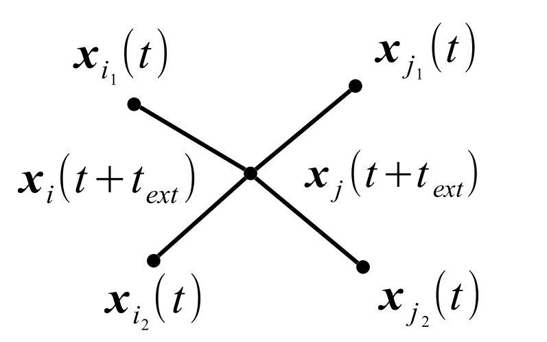
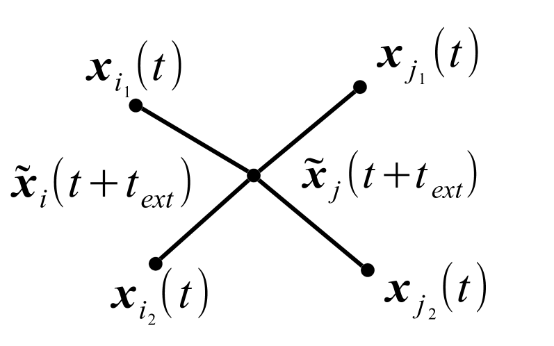
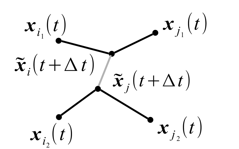
Initially, $\Delta t$ is set equal to a prescribed value of $\Delta t_{0}$. On each time step, the algorithm estimates extinction times for all grain boundaries and selects only those which fall in the interval $[t,t+\Delta t]$. Then the corresponding grain boundaries are sorted according to their extinction times. Next we move along this list and record those boundaries whose vertices have not yet been encountered. This process continues until either all vertices are exhausted, or a boundary with an already recorded vertex has been detected. In the latter case, the process stops and the time step is adjusted to only allow extinction of the boundaries that have been recorded. This ensures that there is spatial separation between topological transitions. Once the time step has been adapted, transitions that involve all recorded boundaries are implemented and the rest of the network is allowed to evolve in a continuous fashion. Then the time step is reset to the original value of $\Delta t_{0}$ and the procedure is repeated until 80% of the grains have been eliminated.

Fig. 3: Configurations resulting in grain removal. The location of the new triple junction $\widetilde{\mathbf{x}}_{1}(t)$ is set to be the collision point for the two triple junctions that collide first.

There are two types of transition events: (1) neighbor switching, and (2) grain removal. From the detection point of view outlined above, these events are indistinguishable. On the other hand, their resolution is completely different. At first, all detected events are considered to be a neighbor switching event, as shown in Fig. 2. However, when one of the two grains adjacent to the disappearing grain boundary has only three sides, we proceed to remove that grain, as depicted in Fig. 3. The neighbor switching is done according to the rules discussed in Section 3. We assume that the anisotropy is small enough so that a shrinking grain boundary cannot be simulatneously adjacent to two 3-sided grains, and return an error if this happens.

Note that only 3-sided grains are allowed to be removed. Thus, for a 5-sided grain to be able to disappear, it needs first to become a 4-sided grain and then a 3-sided grain. The number of sides of a given grain can change either through a neighbor switching event, or as a consequence of a neighboring grain disappearance. Finally, when a switching of neighbors is performed, the length of the new grain boundary is computed to be proportional to $\Delta t-t_{ext}$, where $t_{ext}$ is the extinction time of the grain boundary in question.

7 Numerical convergence study

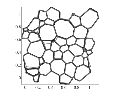
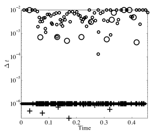
Although a rigorous analytical investigation is beyond the scope of this paper, in this section we present a numerical study subjecting the proposed algorithm to several tests for accuracy and convergence. The first test is designed to check how well the numerical procedure is able to handle topological transitions via time-step adaptation. For this purpose, we compare the results of several simulations using different values of the maximum time step $\Delta t_{0}$ in Figs. 4-5. Fig. 4 shows grain boundary structures obtained from the same initial configuration with $200$ grains at $t=0.45$ when approximately $80\%$ of the grains were removed. Three different simulations with maximum time step sizes $\Delta t_{0}=10^{-2},\ 10^{-5},\mbox{ and }10^{-6}$ were performed. It is evident that, with the exception of the grain structure obtained when $\Delta t_{0}=10^{-2}$—the coarsest maximum time step—all grain boundaries lie directly on top of each other. In Fig. 5 we plot the dependence between the simulation time and the size of time step for $\Delta t_{0}=10^{-2}\mbox{ and }10^{-6}$. The figure shows that fewer time step refinements are performed for smaller $\Delta t_{0}$ and that for a very small $\Delta t_{0}$, refinements are only needed when a grain removal occurs.

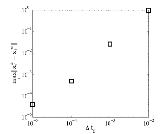
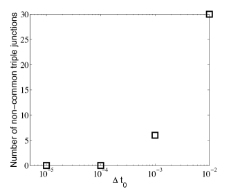
Next we test our algorithm for convergence using the following measures. First we run a set of simulations corresponding to several $\Delta t_{0}$. We consider the simulation with the smallest $\Delta t_{0}=10^{-6}$ as “well-resolved” and benchmark the results of other simulations against it. In Fig. 6 we consider the difference between the positions of triple junctions produced by a given and the well-resolved simulations at to the time $t=0.45$. Only the remaining common junctions are considered in this calculation. It can be seen that the error decreases linearly toward zero as $\Delta t_{0}\to 0$. In fact, the number of non-common triple junctions remaining at the time $t$ decreases to zero as well and it becomes exactly zero when $\Delta t_{0}=10^{-4}$.

These tests allow the conclusion that the proposed algorithm successfully handles both topological transitions and the grain boundary motion and is numerically stable.

Fig. 4: Grain boundary networks evolved from the same configuration with 200 grains up to t=0.45 when approximately 80% of the grains were removed. The simulations were run with three different maximum time steps: $\Delta t_{0}=10^{-2}$ (light grey), $10^{-5}$ (dark grey), and $10^{-6}$ (black).

Fig. 5: Evolution of the timestep for $\Delta t_{0}=10^{-2}$ ($\circ$) and $\Delta t_{0}=10^{-7}$ ($+$). Larger markers represent the instances when the decrease in time step was caused by grain removal in the absence of neighbor switching.

Fig. 6: Deviation between positions of triple junctions corresponding to grain boundary networks for various $\Delta t_{0}$ compared to a well-resolved simulation with $\Delta t_{0}=10^{-7}$. All simulations started from the same initial data and were compared at the same absolute time $t=0.45$.

Fig. 7: Number of non-common triple junctions between grain boundary networks for various $\Delta t_{0}$ and a well-resolved simulation with $\Delta t_{0}=10^{-6}$. All simulations started from the same initial data and were compared at the same absolute time $t=0.45$.

8 Numerical results

8.1 Statistics

In this section we analyze the statistics for networks with isotropic and weakly anisotropic grain boundary energy. In all cases the network is initialized via a Voronoi tessellation using points uniformly distributed in the computational domain and assuming periodic boundary conditions. All networks initially contained $100,000$ grains and were evolved until $80\%$ of the grains were removed.

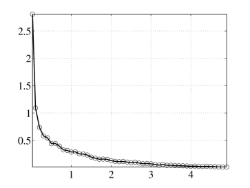
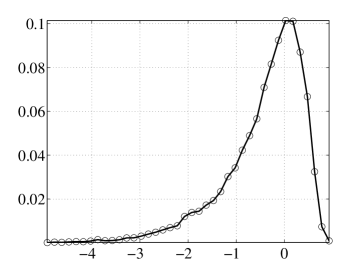
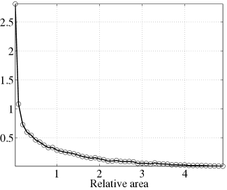
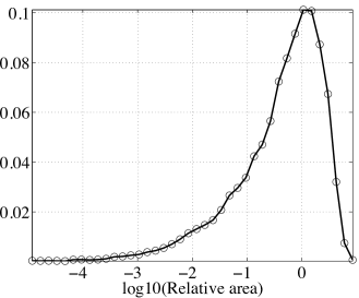
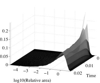
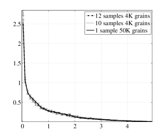
Fig. 8 depicts the relative area distribution using linear and log scales. We observe that the distribution is skewed toward grains with smaller areas (this is emphasized in the log-scale plot). There is a notable difference from statistics produced by a curvature-driven simulation; in fact, grains with smaller areas tend to have a smaller rate of area change (Fig. 18(a)). As the result a grain boundary network evolved via triple junctions motion tends to have more small grains.

(a) linear scale.

(b) log scale.

Fig. 8: Relative grain area distribution in the isotropic network consisting of 20,000 grains that evolved from an initial configuration of 100,000 grains.

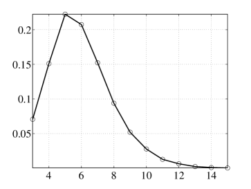
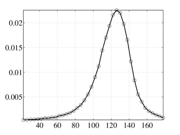
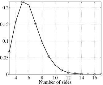
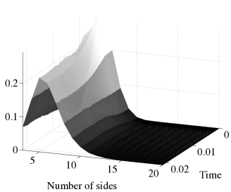
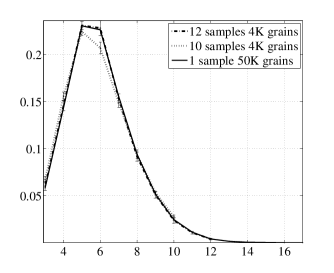
The distribution of the number of sides per grain is shown in Fig. 99(a) and demonstrates a bias toward three-sided grains. We attribute this to the fact that grains need to go through a cascade of decreasing number of sides before they can be removed, i.e., a grain needs to become a three-sided grain before it is allowed to disappear. The largest proportion of grains are five-sided. Another important feature is that when the number of sides exceeds $n=12$, the value of the probability density function is very small compared to the values when $n\leq 12$. This is relevant to understanding statistics presented below because the sample size for large $n$ is small.

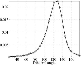
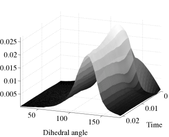
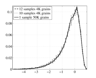
The third statistic (Fig. 99(b)) is the dihedral angle distribution. This distribution does not seem to be centered at $120^{\circ}$ but instead shows a small shift toward angles larger than $120^{\circ}$.

(a)

(b)

Fig. 9: Distributions for the: (a) number of sides of a grain; and (b) dihedral angle. The data is collected using the isotropic network of 20,000 grains that evolved from an initial configuration consisting of 100,000 grains.

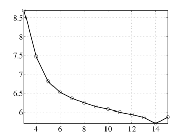
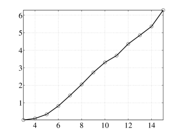
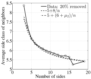
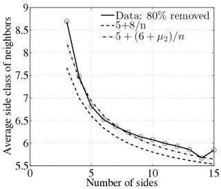
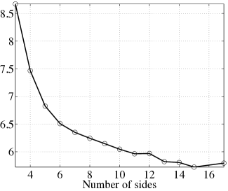
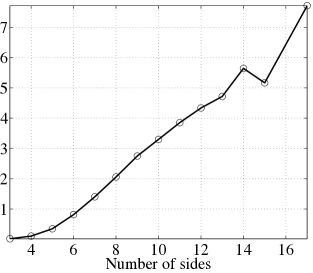
Finally, we computed the average number of sides of neighbors for grains with a given number of sides (Fig. 1010(a)) as well as the reduced average area of the neighbors (Fig. 1010(b)). The comparison to the empirical Aboav and Aboav-Weaire laws [28] is shown in Fig. 11 for the systems from which the 20% and 80% of the grains were removed, respectively. The Aboav-Weaire law appears to provide a better fit in both cases.

(a)

(b)

Fig. 10: For grains with a given number of sides: (a) Average number of sides of neighboring grains; (b) Average relative area of neighboring grains. The data is collected using the isotropic network of 20,000 grains that evolved from an initial configuration consisting of 100,000 grains.

(a)

(b)

Fig. 11: Comparison with Aboav and Aboav-Weaire laws for an isotropic network. (a) $20\%$ of the grains have been removed; (b) $80\%$ of the grains have been removed.

The distributions obtained for grain boundary networks with weakly anisotropic grain boundary energy $\gamma(\Delta\alpha)=0.95-0.05\,\cos^{3}(4\,\Delta\alpha)$ are shown in Figs. 12-14. Note that the statistical features that develop in this case are essentially identical to those observed when the grain boundary energy is isotropic.

(a) linear scale.

(b) log scale.

Fig. 12: Relative grain area distribution in the anisotropic network consisting of 20,000 grains that evolved from an initial configuration of 100,000 grains.

(a)

(b)

Fig. 13: Distributions for the: (a) number of sides of a grain; and (b) dihedral angle. The data is collected using the anisotropic network of 20,000 grains that evolved from an initial configuration consisting of 100,000 grains.

(a)

(b)

Fig. 14: For grains with a given number of sides: (a) Average number of sides of neighboring grains; (b) Average relative area of neighboring grains. The data is collected using the anisotropic network of 20,000 grains that evolved from an initial configuration consisting of 100,000 grains.

8.2 Self-similarity

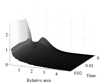
We have tested the distributions we have observed for self-similarity. We found that self-similarity does indeed develop and is very consistent for all distributions of interest. Here a critical issue is that a sufficiently large number of grains is needed initially for a clear trend to develop. In our experience, the statistics do not depend on the details of the initial configuration; these can only affect the time needed to achieve stable statistics. Here the initial set of grains was generated using the Voronoi construction for a uniformly distributed random collection of points in a rectangular domain.

Figs. 15 and 16 show the development of various distributions over time. The plots were produced by evolving grain boundary networks that initially contained $100,000$ grains up until $20,000$ grains remained.

(a)

(b)

Fig. 15: Evolution in time of the relative grain area distribution. The statistics was collected for every time step while evolving grain boundary networks that initially contained $100,000$ grains up until $20,000$ grains remained.

(a)

(b)

Fig. 16: Evolution in time of distributions for the: (a) number of sides of a grain; and (b) dihedral angle. The statistics was collected for every time step while evolving grain boundary networks that initially contained $100,000$ grains up until $20,000$ grains remained.

8.3 Comparison of different neighbor switching rules

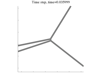
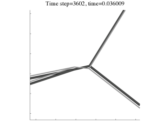
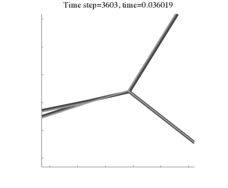
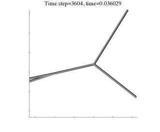
We have compared three types of neighbor switching rules used in the literature: maximum dissipation rate [7], maximum force [10], and the proposed approach. Fig. 17 shows a part of the grain boundary network immediately preceding the first neighbor switching event and for several time steps afterward. The three rules result in a different initial orientation of the newly formed grain boundary that has the length proportional to $\Delta t-t_{ext}$. In all cases, subsequent evolution of the network corrects the angle to the one enforced by the continuous part of the algorithm. Overall, it appears that a “suboptimal” neighbor switching rule leads to accumulating errors that result in a grain boundary network that differs significantly from that produced using the “optimal” rule, starting from the same initial conditions. However, singular behavior of the continuous part of the dynamical system at the time of the neighbor switch, combined with a smaller maximum time step $\Delta t_{0}$, makes this the error less significant, per Fig. 17d. In all cases, the statistical features of the network seem to be unaffected by the type of the rule used.

From our simulations, it also appears that the networks evolving via different neighbor switching rules (or via the same rule, but with a different maximum time step), move through a very similar sequence of configurations in the state space, albeit at different times.

(a)

(b)

(c)

(d)

Fig. 17: Comparison of three neighbor switching rules: Maximum dissipation rate (light gray) [7], maximum force (gray) [10], the approach described in this paper (black). After a short period of time, configurations are essentially indistinguishable when using a small time step.

8.4 Rate of area change for an $N$-sided grain

(a)

(b)

Fig. 18: (a) Average rate of change of grain area vs. the number of sides of the grain. (b) Average grain area vs. the number of sides of the grain.

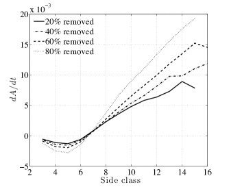
A well-known result for curvature-driven grain growth is the von Neumann-Mullins $(n-6)$-rule. The rule states that, given constant mobility and constant anisotropy, and assuming that the network satisfies the Herring condition (angles between the boundaries meeting at a triple junction are all equal to $120^{\circ}$ in an isotropic case), we have

$$\frac{dA}{dt}=c(n-6),$$

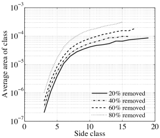
where $c>0$ is a known constant. In a vertex algorithm the $n-6$ rule does not hold. Indeed, in Fig. 18(a) we observe that, although the relation for $n$ between $5$ and $15$ is close to being linear, it is far from that for grains with a smaller number of sides. The distribution depends on time and has a self-similar shape, however the nature of the observed dependence is still an open problem that will be addressed in a future publication. Fig. 18(b) shows that the average area for each class of grains with a given number of sides grows over time. This same behavior is observed in curvature codes [7].

8.5 Stability

We have tested for stability distributions that develop for networks evolving via our algorithm in both isotropic and anisotropic cases. Here we only present the results for the isotropic case due to space constraints and because the conclusions are qualitatively similar.

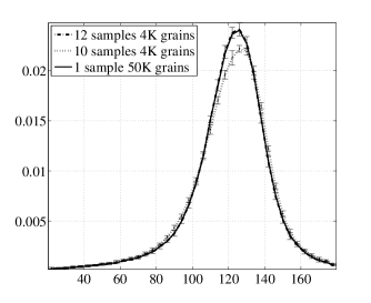
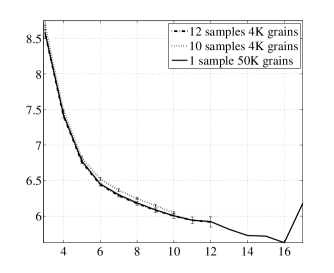
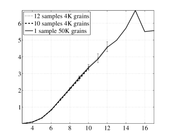
The test has been performed on a sample with $100,000$ grains initially, where the simulation was run until $50\%$ of grains where removed. We decomposed the resulting sample into 12 spatially smaller subsets of equal area and collected various statistics for each sample. These were compared to the output of 10 simulations with initially $20,000$ grains that were run until only $4,000$ were left. The statistics were computed for these smaller samples. We also analyzed the statistics for a single $50,000$ sample.

Fig. 19 through Fig. 21 present the outcome of this study. This experiment shows numerical evidence that all distributions are remarkably stable in the sense that collecting statistics over subareas of the network or the entire network produces the same results.

(a) linear scale.

(b) log scale.

Fig. 19: Stability of the relative grain area distribution. The average of distributions for 12 subsets of the same simulation, the average of distributions for 10 different simulations, and the distribution for one large simulation are shown. The deviation of distributions from their average for each group is indicated by error bars.

(a)

(b)

Fig. 20: Stability of distributions for the: (a) number of sides of a grain; and (b) dihedral angle. The average of distributions for 12 subsets of the same simulation, the average of distributions for 10 different simulations, and the distribution for one large simulation are shown. The deviation of distributions from their average for each group is indicated by error bars.

(a)

(b)

Fig. 21: For the grains with a given number of sides: (a) Average number of sides of neighbors; (b) Average relative grain area of neighbors. The average of distributions for 12 subsets of the same simulation, the average of distributions for 10 different simulations, and the distribution for one large simulation are shown. The deviation of distributions from their average for each group is indicated by error bars.

8.6 Quadruple junctions and their stability

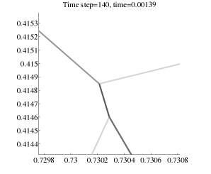
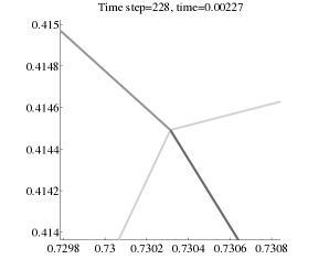
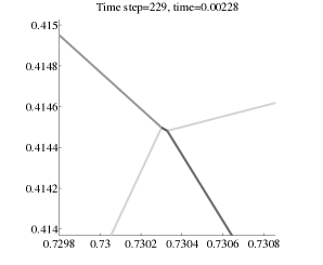
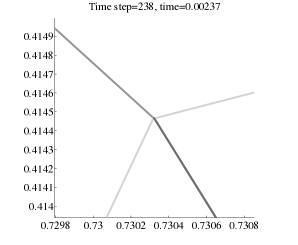
In a network with a large anisotropy stable quadruple junctions may exist. From the implementation point of view, they are two triple junctions that almost overlap. In principle, one needs to develop a separate set of rules that govern neighbor switching for this type of a junction. In our algorithm, quadruple junctions are always assumed to split into triple junctions. However, if a quadruple junction is stable, then any new boundary created as a result of the split would shrink and disappear, restoring the original quadruple junction. In this way, the code is capable of dealing with stable quadruple junctions. The example of such junction in a grain boundary network with an anisotropic grain boundary energy $\gamma(\Delta\alpha)=0.55-0.45\,\cos^{3}(4\,\Delta\alpha)$ is shown in Figs. 22.

(a)

(b)

(c)

(d)

Fig. 22: Evolution of two triple junction that remain together and emulate a quadruple junction. Darker colors correspond to larger grain boundary energy.

9 Conclusions

We have developed a numerical algorithm for an evolving grain boundary network described by a simple vertex model. The model can be formally derived via the assumption that the mobility of triple junctions is much lower than the mobility of grain boundaries evolving via curvature-driven motion. We have used a semi-rigorous analysis of vertex dynamics to derive the neighbor switching rules consistent with continuous evolution of vertices as well as the estimates of vertex collision times. These estimates were incorporated into in the numerical procedure to pinpoint the times corresponding to topological transitions. By simulating coarsening of the vertex model grain boundary network, we have demonstrated that the geometry of configurations that develop is described by the standard statistical measures for characterizing grain growth. These include distributions of relative areas of grains, dihedral angle, number of sides, among others. We have confirmed spatiotemporal stability of the distributions that develop in a network evolving via our numerical algorithm. We find that the distributions are essentially independent of the level of numerical resolution as the network passes through the sequence of similar states. While mesoscopic characteristics of the network appear to be robust, even with respect to changes in the rules governing topological transitions, the microscopic features of the network at a given time are sensitive to any modifications of the algorithm.

10 Acknowledgements

M. E. and C. T. were supported in part by NSF grant DMS-1056821. D. G. was supported in part by NSF grant DMS-1009849. D. K. was supported in part by NSF grants DMS-0806703, DMS-0635983, and OISE-0967140. S. T. was supported in part by NSF grant DMS-1216433.

Appendix 1

Suppose that the edge connecting two vertices ${\bf x}_{i}$ and ${\bf x}_{j}$ disappears at the time $t_{0}$ and that ${\bf p}_{-}$, $\rho$, $\theta$, ${\bf n}$, and $\boldsymbol{\tau}$ are as defined in Section 3. Here we will use (11b) to argue that, as long as $\mathbf{p_{-}}\in C([t_{0}-\Delta t,t_{0}])$ for some small $\Delta t>0$ and

$$\|{\bf p}_{-}(t_{0})\|-2\gamma_{ij}<0,$$

we have that

(26) $$\lim_{t\to t_{0}^{-}}\mathbf{p_{-}}\cdot\boldsymbol{\tau}=0.$$

First, since $\mathbf{p_{-}}\in C([t_{0}-\Delta t,t_{0}])$ and $\|{\bf p}_{-}(t_{0})\|-2\gamma_{ij}<0,$ we can choose $\Delta t$ small enough so that $-4\gamma_{ij}\leq\mathbf{p_{-}}\cdot\mathbf{n}-2\,\gamma_{ij}\leq-\alpha$ on $[t_{0}-\Delta t,t_{0}]$ for some $\alpha>0.$ The system (11b) has a continuous solution on $[t_{0}-\Delta t,t_{0})$ where the function $\rho$ is, in fact, continuous on $[t_{0}-\Delta t,t_{0}]$. Integrating the equation (11a) and using the condition $\rho(t_{0})=0$, we obtain

(27) $$\alpha(t_{0}-t)\leq\rho(t)\leq 4\gamma_{ij}(t_{0}-t),$$

when $t\in[t_{0}-\Delta t,t_{0}]$.

Set ${\mathbf{p}}_{-}=\|{\mathbf{p}}_{-}\|(\cos{\theta_{p}},\sin{\theta_{p}})$, then the equation (11b) takes the form

(28) $$\dot{\theta}=\frac{\|{\mathbf{p}}_{-}\|}{\rho}\sin{(\theta_{p}-\theta)}.$$

We will assume here that ${\mathbf{p}}_{-}\neq{\mathbf{0}}$ on $[t_{0}-\Delta t,t_{0}]$, then both $\|{\mathbf{p}}_{-}\|$ and $\theta_{p}$ are continuous and $\|{\mathbf{p}}_{-}(t)\|>\beta$ for all $t\in[t_{0}-\Delta t,t_{0}]$ and some constant $\beta>0$.

Suppose first that $0\leq\theta_{p}-\theta\leq\pi$ on $[t_{0}-\Delta t,t_{0})$. Then $\dot{\theta}\geq 0$ on $t\in[t_{0}-\Delta t,t_{0})$, hence $\lim_{t\to t_{0}^{-}}\theta$ exists. If this limit is finite, it immediately follows from integrability of the right hand side of (28) and (27) that the $\lim_{t\to t_{0}^{-}}\theta=\theta_{p}(t_{0})$. If the $\lim_{t\to t_{0}^{-}}\theta=\infty$, then the assumption that $\theta_{p}-\theta>0$ implies that $\lim_{t\to t_{0}^{-}}\theta_{p}=\infty$; this violates the continuity of $\theta_{p}$ on $[t_{0}-\Delta t,t_{0}]$. An analogous argument can be used to show a symmetric result for $-\pi\leq\theta_{p}-\theta\leq 0$.

It remains to prove (26) when there exists a sequence $t_{n}\to t_{0}$ such that $t_{n}<t_{n+1}$ and $\sin{\left(\theta_{p}(t_{n})-\theta(t_{n})\right)}=0$ for all $n=1,2,3,\ldots$. Since $\theta_{p}$ is continuous on $[t_{0}-\Delta t,t_{0}]$, we can assume that

(29) $$\left|\theta_{p}(t_{n})-\theta_{p}(t_{0})\right|<\pi/2$$

for all $n=1,2,3,\ldots.$ Fix an arbitrary $n=1,2,3,\ldots$ then $\sin{\left(\theta_{p}(t_{n})-\theta(t_{n})\right)}=0$ and $\sin{\left(\theta_{p}(t_{n+1})-\theta(t_{n+1})\right)}=0$. Assume that $\theta_{p}(t_{n})=\theta(t_{n})$ and $0<\theta_{p}(t)-\theta(t)<\pi$ on the interval $(t_{n},t_{n+1})$. Then the equation (28) guarantees that $\dot{\theta}>0$ on $(t_{n},t_{n+1})$ and thus $\theta$ is increasing on $(t_{n},t_{n+1})$. Further, we have that either $\theta_{p}(t_{n+1})=\theta(t_{n+1})$ or $\theta_{p}(t_{n+1})=\theta(t_{n+1})+\pi$. But since $\theta$ is increasing on the interval $(t_{n},t_{n+1})$, the inequality (29) implies that

$$0\leq\theta_{p}(t_{n+1})-\theta(t_{n+1})=\theta_{p}(t_{n+1})-\theta_{p}(t_{n})+\theta(t_{n})-\theta(t_{n+1})<\theta_{p}(t_{n+1})-\theta_{p}(t_{n})\leq\frac{\pi}{2}.$$

and therefore $\theta_{p}(t_{n+1})=\theta(t_{n+1})$. The same conclusion holds if we assume that $-\pi<\theta_{p}(t)-\theta(t)<0$ on the interval $(t_{n},t_{n+1})$, except that in this case $\theta$ is monotone decreasing on $(t_{n},t_{n+1})$. It follows by an induction argument that $\theta$ and $\theta_{p}$ have the same values at $t_{n}$ and $\theta$ is monotone on $(t_{n},t_{n+1})$ for every $n=1,2,3,\ldots$. The fact that $\lim_{t\to t_{0}^{-}}\theta=\theta_{p}(t_{0})$ is then a simple consequence of continuity of $\theta_{p}$ on $[t_{0}-\Delta t,t_{0}]$. This, in particular, implies (26).

Appendix 2

Here we derive the equation (25), that is, given

(30) $$\Phi(\alpha,x)=\prod_{j=1}^{\lfloor x\rfloor-1}\left|1-\frac{\alpha}{1-\frac{j}{x}}\right|=\prod_{j=1}^{\lfloor x\rfloor-1}\left|\frac{x-j-\alpha x}{x-j}\right|,$$

where $x$ is large and $0<\alpha<1$, we show that

(31) $$\Phi(\alpha,x)=\frac{1}{\pi}\frac{\Gamma(1+x-\lfloor x\rfloor)\Gamma((1-\alpha)x)\Gamma(\lfloor x\rfloor-x+\alpha x)}{\Gamma(x)}\sin{\pi\left((1-\alpha)x-\lfloor(1-\alpha)x\rfloor\right)}.$$

First, given $\lambda>0$, the following relationship

(32) $$\frac{\Gamma(m+\lambda+1)}{\Gamma(l+\lambda)}=\prod_{i=l}^{m}(i+\lambda)$$

holds for any $l,m\in\mathbb{N}$. By changing the index, $j\to\lfloor x\rfloor-j$, we have that

(33) $$\begin{split}\Phi(\alpha,x)&=\prod_{j=1}^{\lfloor x\rfloor-1}\left|\frac{x-\lfloor x\rfloor-\alpha x+j}{x-\lfloor x\rfloor+j}\right|\\ &=\frac{\prod_{j=1}^{\lfloor x\rfloor-\lfloor(1-\alpha)x\rfloor-1}\left(x-\lfloor x\rfloor-\alpha x+j\right)\prod_{j=\lfloor x\rfloor-\lfloor(1-\alpha)x\rfloor}^{\lfloor x\rfloor-1}\left(x-\lfloor x\rfloor-\alpha x+j\right)}{\prod_{j=1}^{\lfloor x\rfloor-1}\left(x-\lfloor x\rfloor+j\right)}\\ &=\frac{\Phi_{1}(\alpha,x)\Phi_{2}(\alpha,x)}{\Phi_{3}(\alpha,x)}.\end{split}$$

We consider $\Phi_{1},\ \Phi_{2},$ and $\Phi_{3}$ separately. Using (32), we immediately obtain

$$\Phi_{3}(\alpha,x)=\prod_{j=1}^{\lfloor x\rfloor-1}\left(x-\lfloor x\rfloor+j\right)=\frac{\Gamma(x)}{\Gamma(1+x-\lfloor x\rfloor)}.$$

By changing the index $j\to j-\lfloor x\rfloor+\lfloor(1-\alpha)x\rfloor$, we find

$$\Phi_{1}(\alpha,x)=\prod_{j=0}^{\lfloor(1-\alpha)x\rfloor-1}\left((1-\alpha)x-\lfloor(1-\alpha)x\rfloor+j\right)=\frac{\Gamma((1-\alpha)x)}{\Gamma((1-\alpha)x-\lfloor(1-\alpha)x\rfloor)},$$

and by changing the index $j\to\lfloor x\rfloor-\lfloor(1-\alpha)x\rfloor-1-j$, we determine that

$$\Phi_{2}(\alpha,x)=\prod_{j=0}^{\lfloor x\rfloor-\lceil(1-\alpha)x\rceil-1}\left(\lceil(1-\alpha)x\rceil-(1-\alpha)x+j\right)=\frac{\Gamma(\lfloor x\rfloor-x+\alpha x)}{\Gamma(\lceil(1-\alpha)x\rceil-(1-\alpha)x)}.$$

It follows by the properties of the $\Gamma$-function that

$$\begin{split}\Phi_{1}(\alpha,x)\Phi_{2}(\alpha,x)=\frac{\Gamma((1-\alpha)x)\Gamma(\lfloor x\rfloor-x+\alpha x)}{\Gamma((1-\alpha)x-\lfloor(1-\alpha)x\rfloor)\Gamma(\lceil(1-\alpha)x\rceil-(1-\alpha)x)}\\ =\frac{\Gamma((1-\alpha)x)\Gamma(\lfloor x\rfloor-x+\alpha x)}{\Gamma((1-\alpha)x-\lfloor(1-\alpha)x\rfloor)\Gamma(1-((1-\alpha)x-\lfloor(1-\alpha)x\rfloor))}\\ =\frac{1}{\pi}\Gamma((1-\alpha)x)\Gamma(\lfloor x\rfloor-x+\alpha x)\sin{\pi\left((1-\alpha)x-\lfloor(1-\alpha)x\rfloor\right)}.\end{split}$$

Dividing this expression by $\Phi_{3}$, we recover (30).

References

- [1] W. Smith and J. Hashemi, Foundations of Materials Science and Engineering. McGraw-Hill series in materials science and engineering, McGraw-Hill, 2003.
- [2] K. Barmak, E. Eggeling, R. Sharp, S. Roberts, T. Shyu, T. Sun, B. Yao, S. Ta’asan, D. Kinderlehrer, A. Rollett, and K. Coffey, “Grain growth and the puzzle of its stagnation in thin films: A detailed comparison of experiments and simulations,” Materials science forum, vol. 715-716, pp. 473–479, 2012.
- [3] R. L. Fullman, “Metal interfaces,” American Society for Metals, Metals Park, OH, 1952.
- [4] H. Frost, C. Thompson, C. Howe, and J. Whang, “A two-dimensional computer simulation of capillarity-driven grain-growth preliminary results,” Scripta Metall., vol. 22, pp. 65–70, 1988.
- [5] T. Nagai, S. Ohta, K. Kawasaki, and T. Okuzono, “Computer simulation of cellular pattern growth in two and three dimensions,” Phase Transitions, vol. 28, p. 177, 1990.
- [6] R. Henseler, B. Niethammer, and F. Otto, “A reduced model for simulating grain growth,” International Series of Numerical Mathematics, vol. 147, pp. 177–187, 2003.
- [7] D. Kinderlehrer, I. Livshits, G. Rohrer, S. Ta’asan, and P. Yu, “Mesoscale simulation of the evolution of the grain boundary character distribution,” Materials Science Forum, vol. 467-470, pp. 1063–1068, 2004.
- [8] D. Weygand, Y. Brechet, and J. Lepinoux, “A vertex dynamics simulation of grain growth in two dimensions,” Philosophical Magazine B, vol. 78, pp. 329–352, 1998.
- [9] D. Weygand, Y. Brechet, and J. Lepinoux, “Mechanisms and kinetics of recrystallisation: A two dimensional vertex dynamics simulation,” Interface Sci., vol. 9, pp. 311–317, 2001.
- [10] L. Barrales-Mora, “2D vertex modeling for the simulation of grain growth and related phenomena,” Mathematics and Computers in Simulation, vol. 80, pp. 1411–1427, 2010.
- [11] M. Syha and D. Weygand, “A generalized vertex dynamics model for grain growth in three dimensions,” Modelling and Simulations in Materials Science and Engineering, vol. 18, p. 015010, 2010.
- [12] D. Weaire and J. P. Kermode, “Computer simulation of a two-dimensional soap froth I. Method and motivation,” Phil. Mag. B, vol. 48, p. 245?259, 1983.
- [13] D. Weaire and J. P. Kermode, “Computer simulation of a two-dimensional soap froth II. Analysis of results,” Phil. Mag. B, vol. 50, pp. 379–395, 1984.
- [14] J.-M. Zhang, K.-W. Xu, and V. Ji, “Experiment and simulation of grain growth in a bidimensional polycrystalline film,” Applied surface science, vol. 218, no. 1, pp. 268–275, 2003.
- [15] C. Sinclair, D. Weygand, J. Lepinoux, and Y. Brechet, “Simulating the topology of recrystallisation in stabilized ferritic stainless steels,” Mater. Sci. Forum, vol. 467-470, pp. 671–676, 2004.
- [16] D. Weygand, J. Lepinoux, and Y. Brechet, “On the nucleation of abnormal grain growth: A 2d vertex simulation,” Materials Science Forum, vol. 467 – 470, pp. 1123–1128, 2004.
- [17] W. W. Mullins, “The statistical selfsimilarity hypothesis in grain growth and particle coarsening,” J. of Applied Physics, vol. 59, p. 1341, 1986.
- [18] A. Harun, E. A. Holm, M. P. Clode, and M. A. Miodownik, “On computer simulation methods to model Zener pinning,” Acta Materialia, vol. 54, no. 12, pp. 3261 – 3273, 2006.
- [19] D. Molodov, Microstructural Design of Advanced Engineering Materials. Wiley, 2013.
- [20] K. Barmak, M. Emelianenko, D. Golovaty, D. Kinderlehrer, and S. Ta’asan, “A new perspective on texture evolution,” Intl. J. of Num. Anal. and Modeling, vol. 5, Supp, pp. 93–108, 2008.
- [21] K. Barmak, M. Emelianenko, D. Golovaty, D. Kinderlehrer, and S. Ta’asan, “Towards a statistical theory of texture evolution in polycrystals,” SIAM J. Sci. Comput., vol. 30, no. 6, pp. 3150–3169, 2008.
- [22] K. Barmak, E. Eggeling, M. Emelianenko, Y. Epshteyn, D. Kinderlehrer, R. Sharp, and S. Ta’asan, “Critical events, entropy, and the grain boundary character distribution,” Phys. Rev. B, vol. 83, p. 134117, 2011.
- [23] W. Mullins, Solid Surface Morphologies Governed by Capillarity, pp. 17–66. Metal Surfaces: Structure, Energetics and Kinetics, Cleveland Ohio: ASM, 1963.
- [24] W. Mullins, “2-Dimensional motion of idealized grain growth,” Journal Applied Physics, vol. 27, no. 8, pp. 900–904, 1956.
- [25] C. Herring, “The use of classical macroscopic concepts in surface energy problems,” in Structure and Properties of Solid Surfaces, pp. 5–81, 1953.
- [26] D. Kinderlehrer and C. Liu, “Evolution of grain boundaries,” Mathematical Models and Methods in Applied Sciences, vol. 11, pp. 713–729, Jun 2001.
- [27] S. Esedoglu and F. Otto, “Threshold dynamics for networks with arbitrary surface tensions,” Communications on Pure and Applied Mathematics, 2013.
- [28] C. V. Thompson, “Grain growth and evolution of other cellular structures-iii. grain growth in two dimensions,” Solid State Physics-Advances in Research and Applications, vol. 2001, no. 55, pp. 272–278, 2000.
Appendix 1
Suppose that the edge connecting two vertices and disappears at the time and that , , , , and are as defined in Section 3. Here we will use (11b) to argue that, as long as for some small and