Comparisons of Two- and Three-Dimensional Convection in Type I X-ray Bursts

Abstract

We perform the first detailed three-dimensional simulation of low Mach number convection preceding runaway thermonuclear ignition in a mixed H/He X-ray burst. Our simulations include a moderate-sized, approximate network that captures hydrogen and helium burning up through rp-process breakout. We look at the difference between two- and three-dimensional convective fields, including the details of the turbulent convection.

1 Introduction

X-ray bursts (XRBs) are the thermonuclear runaway in a H/He layer on the surface of a neutron star. These transient events can be used to probe the structure of neutron stars and the equation of state of dense material (Steiner et al., 2010; Özel et al., 2010). Furthermore, they are also the sites of rp-process nucleosynthesis (Schatz et al., 2001). For these reasons, understanding the dynamics of the explosion has seen substantial research interest in the past years.

One-dimensional studies (Taam, 1980; Taam et al., 1996; Woosley et al., 2004) can reproduce the observed energies, durations, and recurrence timescales for XRBs, but use a parameterized model for convection, namely mixing length theory (which likely does not describe turbulent convection accurately e.g. Arnett et al. 2015). An open question is whether a fully-turbulent convective velocity field can modify the nucleosynthesis. Additionally, the convection may dredge up heavy element ash to the photosphere (in ’t Zand & Weinberg, 2010; Bhattacharyya et al., 2010) thereby altering the opacity of the atmosphere, which affects the inference of neutron star mass and radius from photospheric radius expansion (PRE) bursts. These are inherently three-dimensional problems.

Previously, we performed two-dimensional simulations, focusing first on pure He bursts (Malone et al., 2011), and then later on mixed H/He bursts (Malone et al., 2014). The latter study used an approximate network to capture the hot-CNO, triple-$\alpha$, and initial rp-process breakout burning. There we found that we needed a spatial resolution of about 6 cm zone^-1 in order to accurately model the burning; for comparison, the extremely temperature-sensitive burning of the pure He models of Malone et al. (2011) required 0.5 cm zone^-1 resolution. In this paper, we extend our studies by performing the first three-dimensional model of convective burning in a H/He XRB, using the reaction network from Malone et al. (2014). This initial study compares to our two-dimensional results, and discusses the computational requirements for a more extensive study.

2 Numerical Method

We use the publicly-available MAESTRO code (Nonaka et al., 2010), which solves the equations of low Mach number hydrodynamics by reformulating the reactive Euler equations to filter soundwaves while retaining compressibility effects due to stratification and local heat release. By filtering dynamically unimportant soundwaves, MAESTRO enables efficient simulation of slow convective flows, such as those in XRBs (Malone et al., 2011, 2014), various progenitors of Type Ia supernovae (Zingale et al., 2011; Nonaka et al., 2012; Zingale et al., 2013), and in the cores of massive stars (Gilet et al., 2013). Also important for simulations like these is that the low Mach number formulation analytically enforces hydrostatic equilibrium of the base state, allowing us to maintain a hydrostatic atmosphere in the simulation code without the development of large spurious velocities (see, e.g., Zingale et al. 2002).

All of the MAESTRO options and microphysics used in our two-dimensional study of XRBs in Malone et al. (2014) are retained for this study. In particular, we use the new energy formulation variant of MAESTRO, based on the ideas in Klein & Pauluis (2012) and Vasil et al. (2013), which improves energy conservation and our treatment of gravity waves. We use the Helmholtz equation of state (EOS) from Timmes & Swesty (2000), which includes an ideal gas of nuclei, a photon gas, and an electron/positron gas with arbitrary degeneracy and relativistic parameters, and Coulomb corrections. MAESTRO is under continuous development, and we’ve improved the advection portion of the code since the construction of the interface states was last discussed in Almgren et al. (2008). We take the opportunity to document those changes in Appendix A.

We use the same parametrized initial model as in our two-dimensional study. Briefly, the model consists of a $M=1.4~{}M_{\odot}$, $R=10$ km neutron star, of which we model the outer $\sim 1.4\times 10^{3}$ cm as an isothermal ($T=3\times 10^{8}$ K), pure ${}^{56}\mathrm{Ni}$ gas. On top of the neutron star is a warm accreted layer of mainly H/He fuel that is slightly metal-rich compared to solar, with CNO metals tied up in ${}^{14}\mathrm{O}$ and ${}^{15}\mathrm{O}$ in a ratio comparable to their respective $\beta$-decay lifetimes. A smooth transition is applied between the density ($\rho=2\times 10^{6}$ g cm^-3) and temperature ($T=9.5\times 10^{8}$ K) at the base of the accreted layer and the surface of the neutron star. The accreted layer is given an isentropic profile, making it convectively unstable, and the temperature decreases until a cutoff temperature is reached. The original extent of the convective region is $\lesssim 2\times 10^{3}$ cm. 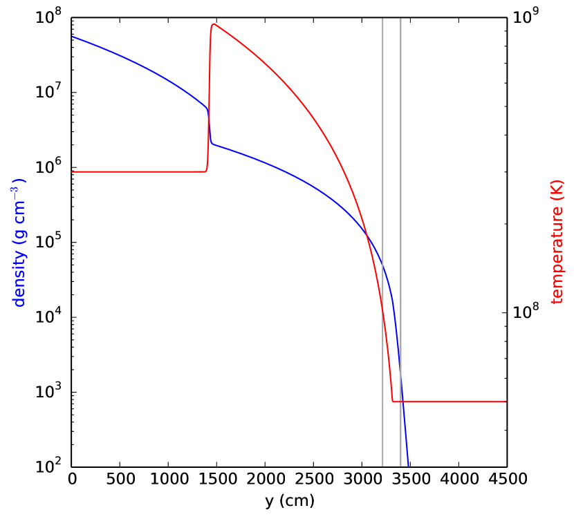Figure 1 shows the density and temperature profile, along with the values of the cutoff densities that are part of the MAESTRO algorithm. For the three-dimensional simulations present here, the anelastic and base cutoff densities have been increased slightly to $2\times 10^{3}~{}\mathrm{g~{}cm^{-3}}$ to better quench the dynamics above the atmosphere. The two-dimensional simulations used the same parameters as in Malone et al. (2014). The reader is referred to the Appendix of Malone et al. (2014) for more details of our model construction procedure. Finally we note that all of the problem setup files, inputs, and initial models for the runs presented here have been copied into the main MAESTRO code repository in Exec/SCIENCE/xrb_mixed/, allowing anyone to rerun these simulations.

In this paper, we perform two three-dimensional simulations to assess the dynamics of the convective flow. We model the XRB using a plane-parallel geometry. Our wide simulation uses a uniform grid of $512\times 512\times 768$ and our narrow simulation uses a grid of $256\times 256\times 768$ zones, both with 6 cm zone^-1 spatial resolution—the same resolution used in our two-dimensional study. As the simulation evolves, the one-dimensional hydrostatic base state that MAESTRO carries is allowed to expand due to the heating, following the procedure described in Almgren et al. (2006).

2.1 Correction to the Network

Our reaction network contains 10 species, approximating hot CNO, triple-$\alpha$, and rp-breakout burning up through ${}^{56}\mathrm{Ni}$, using the ideas from Wallace & Woosley (1981), but with modern reaction rates from ReacLib (Cyburt et al., 2010) where available (see the discussion in Malone et al. 2014 for more details). This is the same network used in Malone et al. (2014), but with one important change. The convective flow field in Malone et al. (2014) showed signs of splitting into two distinct convective regions (e.g. Figure 7 of that paper). The split occured at a location of a secondary peak in energy generation, which grew with time (Figure 9 in that paper). We attributed this extra energy to the branching ratio, $\lambda_{1}$, of $\beta$-decay versus $\alpha$-capture on ${}^{18}\mathrm{Ne}$ as a breakout mechanism from the Hot CNO cycle. The precise location of the secondary peak in energy production was where the branching ratio favored the $\beta$-decay to ${}^{18}\mathrm{F}$ (see Figure 10 of Malone et al. 2014), followed by ${}^{18}\mathrm{F}\left(\mathrm{p},\alpha\right){}^{15}\mathrm{O}$; the approximate network converts ${}^{17}\mathrm{F}$$+2$p directly to ${}^{15}\mathrm{O}$$+\alpha$ at a rate governed by the rate of p-capture on ${}^{17}\mathrm{F}$ and $\lambda_{1}$.

This coincidence of peak energy generation and $\lambda_{1}$ transition was a red herring: the energy generation from the ${}^{17}\mathrm{F}$$\left(2\mathrm{p},\alpha\right)$${}^{15}\mathrm{O}$ chain was insufficient to reproduce the production rate we witnessed. We know now that we erroneously had an additional term in the reaction network — based on legacy code — that attempted to model p-capture on ${}^{56}\mathrm{Ni}$ to heavier elements. In particular, there was a kludge of a term involving ${}^{56}\mathrm{Ni}+56\mathrm{p}\rightarrow 2\,{}^{56}\mathrm{Ni}$ to mimic the energy release of heavier element production, which should not have been included in the network. This “reaction” occured exactly at the secondary peak in energy generation and depletion of H, and its rate was sufficient to reproduce the energy production and its increase with time. We have since removed this feature of our network. All calculations in this paper, including the 2-d comparisons, use the corrected network, which is available in the MAESTRO distribution in Microphysics/networks/rprox/.

3 Results

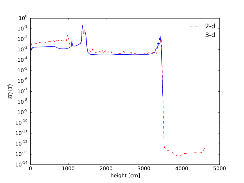
In order to understand how dimensionality affects our results, we compare to updated two-dimensional calculations based on Malone et al. (2014). In particular, we use a 6 cm resolution $1024\times 768$ zone calculation. Figure 2 shows the standard deviation of temperature (compared to other zones at the same height) as a function of height for the two- and three-dimensional runs, both at $t=0.02$ s. The overall trend is the same for the two calculations, with the magnitude of the temperature fluctuations in the convective region ($\sim$ 1400 cm to 3550 cm) $\delta T/\langle T\rangle\sim 10^{-3}$ to $10^{-4}$.

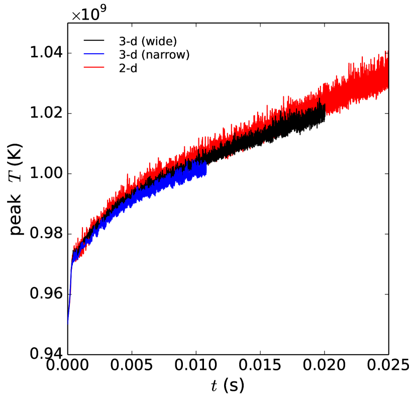
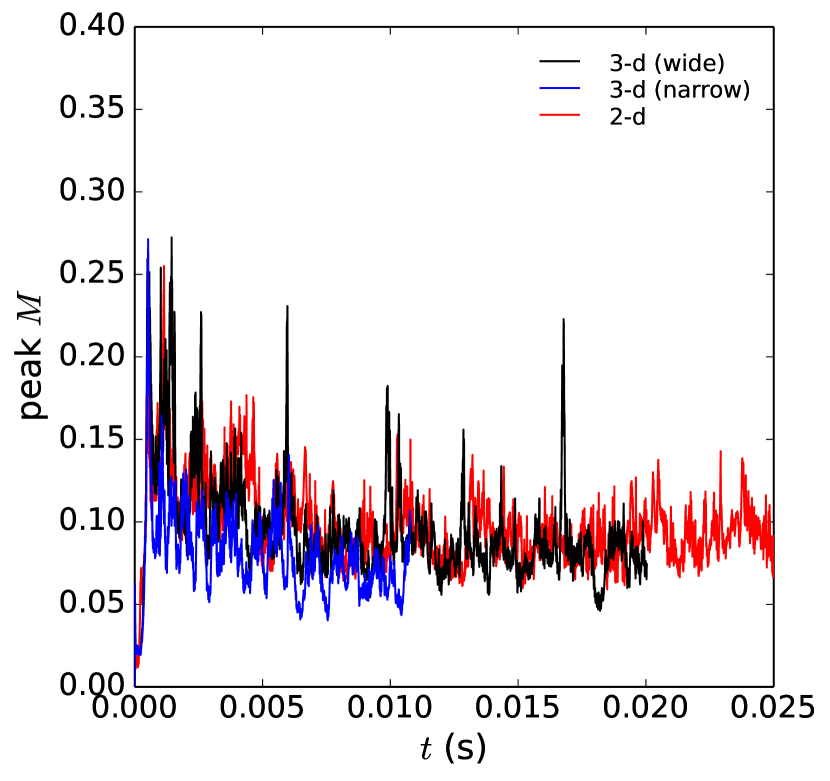
Figure 3 shows the peak temperature and peak Mach number as a function of time for the runs. We see that they closely track one another, but that in the wide three-dimensional simulation there more sporatic spikes to moderate Mach number throughout the simulation. At the start of the calculation, there is always a period of transient behavior as the heating needs to set up a consistent convective velocity field, but the flow quickly settles down. For both simulations, the average Mach number after the transient is about 0.1; in the longer-duration two-dimensional case, the Mach number asymptotes to 0.1. The temperature plots all track one another well. We did not run the three-dimensional calculation as long as the two-dimensional calculation, to conserve computational resources.

It is interesting to note how the peak Mach number translates into a timestep improvement compared to a fully compressible code. For this problem, the sound speed in the atmosphere is greater the deeper one goes into the atmosphere, but the Mach number is highest at the top of the atmosphere. As a result, the timestep increase will actually be better than the naive $1/M$ one would expect if the domain were uniform. A further complication is that, in the compressible code, when we reach the low density material at the top of the atmosphere that buffers us from the boundary, it is radiation pressure that dominates here, articially increasing the hydrodynamic soundspeed. This is a common limitation that arises from using an EOS that includes radiation instead of modeling the radiation field itself. For comparison, we started the same XRB simulation (in two dimensions) in the Castro code (Almgren et al., 2010), and the average timestep after $2.76\times 10^{-4}$ s of evolution was $\Delta t_{\mathrm{comp}}=2.79\times 10^{-10}$ s. For the main three-dimensional MAESTRO calculation, the average timestep over the course of the entire simulation was $\Delta t_{\mathrm{LM}}=1.93\times 10^{-7}$ s—a $\sim 700\times$ improvement.

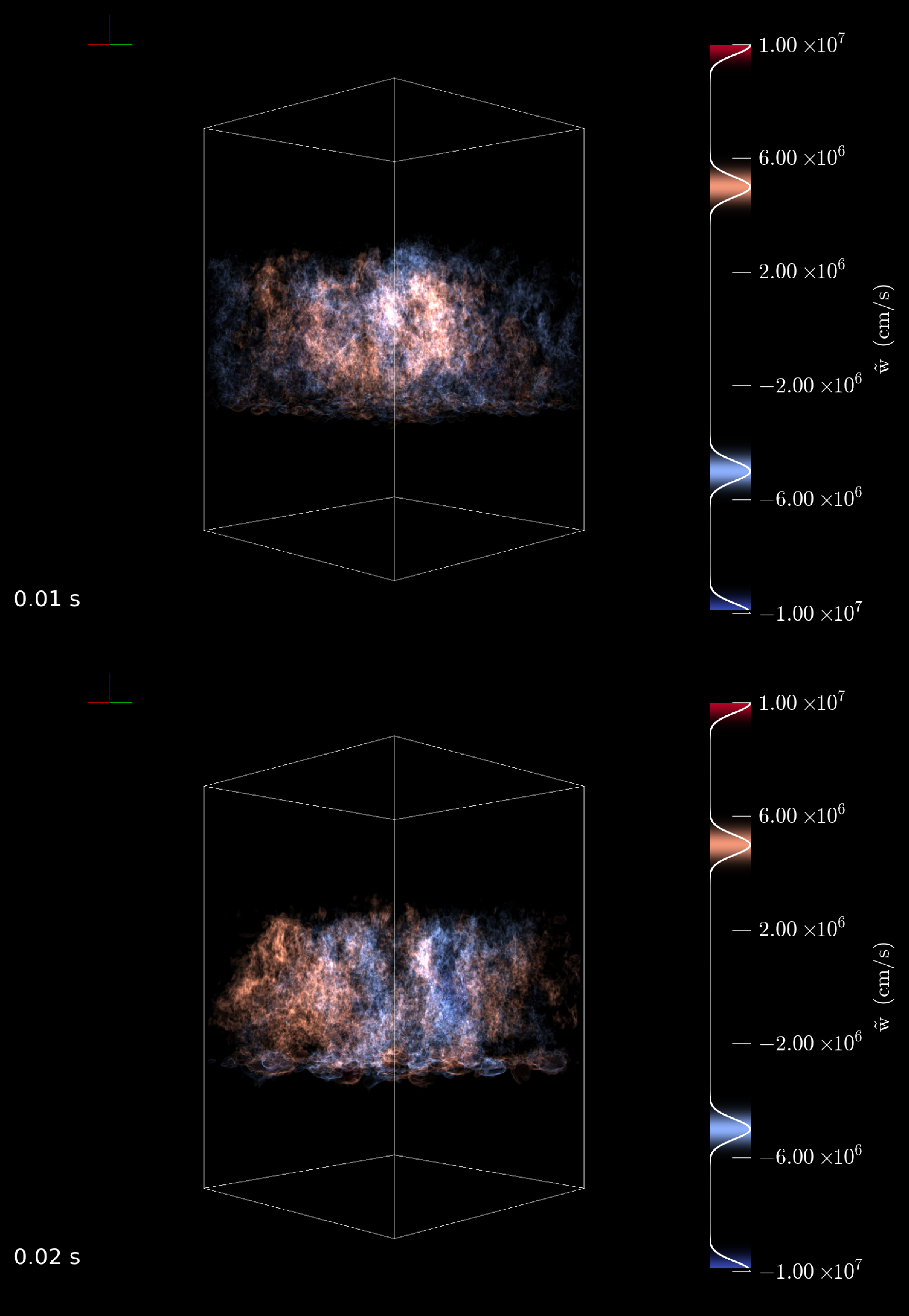
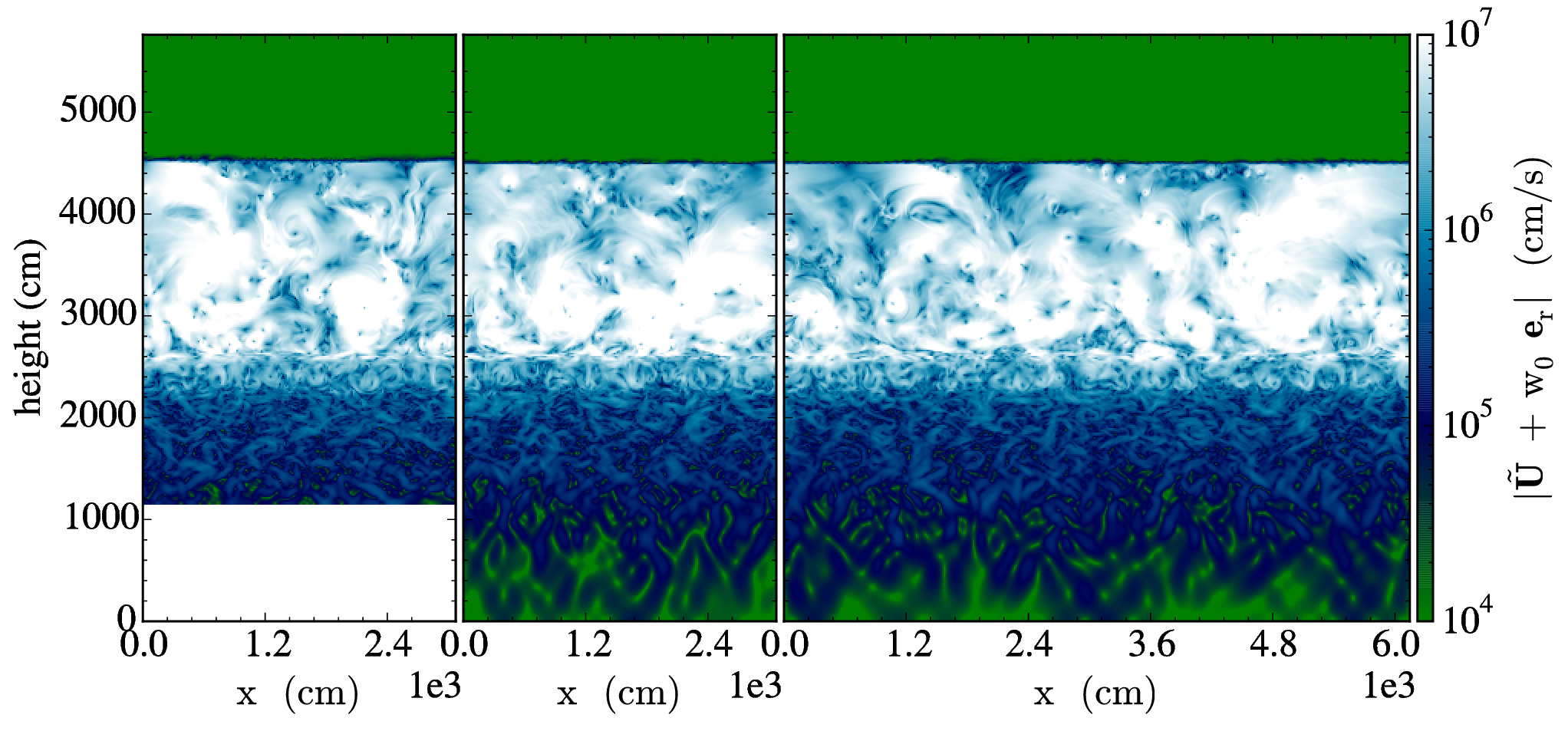
The convective velocity structure of the wide three-dimensional simulation is shown in Figure 4, highlighting the vertical velocity. These two images are representative of the flow throughout the simulation. We do not see the tight layering that was apparent in the older two-dimensional simulations (especially for narrower domains; see Figures 6 and 7, and the discussion in Section 4.2.1 of Malone et al. 2014) because of the fix to the reaction network discussed in Section 2.1. To better understand the difference in the nature of the convective flow, we need to examine the turbulent structure.

Turbulence is known to behave differently between two and three dimensions (see, e.g. Ouellette 2012). To get a feel for the turbulent nature of the convection in these simulations, we look at the kinetic energy power spectrum. Following the discussion regarding turbulence in stratified flows in Nonaka et al. (2012) and references therein, we calculate a generalized kinetic energy density spectrum as

$$E_{n}(k)=\frac{1}{\Omega}\int_{\mathbf{S}({\bf{k}})}\frac{1}{2}{\bf{\widehat{V}}}_{n}({\bf{k}})\cdot{\bf{\widehat{V}}}_{n}^{\star}({\bf{k}})d\mathbf{S},$$ (1)

where ${\bf{\widehat{V}}}_{n}({\bf{k}})$ is the Fourier transform of ${\bf{V}}_{n}({\bf{x}})=\rho^{n}({\bf{x}})\widetilde{{\bf{U}}}({\bf{x}})$ with $n$ specifying the density weighting, $\mathbf{S}({\bf{k}})$ is the surface defined by $|{\bf{k}}|=k$, and the $\star$ denotes complex conjugation. We note that here we use $\widetilde{{\bf{U}}}$, the local velocity on the grid, instead of explicitly calculating the turbulent velocity fluctuations from the full velocity field, including the base state expansion, ${\bf{U}}=\widetilde{{\bf{U}}}+w_{0}{\bf{e}}_{r}$, because $\widetilde{{\bf{U}}}$ is essentially the velocity perturbations on top of an otherwise hydrostatic background state (Nonaka et al., 2010). The volume, $\Omega$, and surface element, $d\mathbf{S}$, are based on the dimensionality of the problem. The goal is to find the proper scaling of the energy density spectrum with wavenumber for both two- and three-dimensional flow.

The units of ${\bf{\widehat{V}}}_{n}$ are [gⁿ cm^1+D-3n s^-1], where the extra power of $D$ on the length scale comes from the integral over $d{\bf{x}}$ in the definition of the Fourier transform. In Equation (1), the integral is done in $k$-space, such that $d\mathbf{S}\sim d^{D-1}k$ with units [cm^1-D], whereas the normalization is in real-space, so that $\Omega$ has units of [cm^D]. Upon integration of Equation (1), the dimensionality, $D$, drops out of the equation, and the units of the generalized kinetic energy density spectrum become [g²ⁿ cm^3-6n s^-2] for both two- and three-dimensional configurations. For turbulent flows that have density variation (i.e. compressible or stratified flows), the typical Kolmogorov energy dissipation rate, $\epsilon(l)$, at a given length scale $l$ should be weighted by the mass density (see Fleck, 1983, 1996, for example): $\epsilon(l)=\rho U^{3}(l)/l$, which has units of [g cm^-1 s^-1]. The arguments of Nonaka et al. (2012) then apply to any dimension: the only combination of $\epsilon^{\alpha}k^{\beta}E_{n}(k)$ that yields a dimensionless quantity is when $\alpha=-2/3$, $n=1/3$, and $\beta=5/3$. If the physics of two dimensional and three dimensional turbulence were the same (this is likely not the case), then the spectrum defined in Eq. (1) should scale as $k^{-5/3}$ for both two- and three-dimensional flows.

In evaluating Eq. (1), we create equally-spaced radial wavenumber bins, $k_{i}$, ranging from the smallest physical wavenumber, $1/L$, to the highest meaningful wavenumber, $1/(2\Delta x)$, where $L$ is the domain width. The Fourier transform of the kinetic energy density gives us

$$\hat{K}(k_{x},k_{y},k_{z})=\frac{1}{2}({\bf{\widehat{V}}}_{n}\cdot{\bf{\widehat{V}}}_{n}^{\star})$$ (2)

For each of points in the three-dimensional $\hat{K}$ array, we define $|k|=\sqrt{k_{x}^{2}+k_{y}^{2}+k_{z}^{2}}$ and determine which of the radial bins, $k_{i}$, this falls into and add the value of $\hat{K}$ to that bin’s sum. Done this way, we are integrating up in spherical shells in $k$-space, using our discrete bins. The same procedure is done in two dimensions, but now we are working in the $k_{x}$-$k_{y}$ plane, and are integrating up over annular regions in that plane, again defined by our discrete bins, $k_{i}$. We do not worry about the $1/\Omega$ normalization, since we will normalize each spectrum such that its peak value is 1.

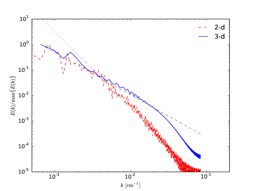
Figure 5 shows the power spectrum of the two-dimensional and wide three-dimensional XRB simulations at $t=0.02$ s. For this analysis, we restrict the domain to just the vicinity of the convective region, including only the vertical range $1300~{}\mathrm{cm}<z<3550~{}\mathrm{cm}$. For the three-dimensional case, we see that we have more than a decade in wavenumber where we achieve a $k^{-5/3}$ power-law scaling, indicative of Kolmogorov turbulence. We note that the region we are studying is not periodic in the vertical direction, but an FFT assumes periodicity, so the discontinuity through the vertical boundary may affect the behavior at high wavenumbers, perhaps accounting for the slow fall in the three-dimensional spectrum. For the two-dimensional case, the spectrum starts off with a $k^{-5/3}$ scaling, but then becomes steeper at moderate wavenumbers. Such a break in the power law scaling for two-dimensional turbulence is predicted for very idealized turbulence where the steeper part of the curve has a $k^{-3}$ scaling attributed to a cascade of enstrophy (e.g.  Kraichnan, 1967; Leith, 1968; Batchelor, 1969). Numerical simulation cannot achieve the idealized conditions (e.g. infinte domain and infinite Reynolds number) assumed in the $k^{-3}$ derivation, and sometimes achieve a steeper power law (e.g. the review by Gkioulekas & Tung, 2006, and references therein). In our two-dimensional simulation, we see a moderate range in the spectrum after the break consistent with $k^{-3}$.

We have also seen such a difference in scaling between two- and three-dimensional turbulence on smaller scales in reactive Rayleigh-Taylor simulations (Zingale et al., 2005), where we saw a spectrum that appeared to follow the $k^{-11/5}$ scaling predicted by Bolgiano-Obukhov statistics for a two-dimensional cascade (Niemeyer & Kerstein, 1997). In that study, we found that a wide domain, giving more statistics, was essential to see this scaling. The difference in the scaling we observe in the present simulations suggests that there is a fundamental difference in how the cascade takes place between the two- and three-dimensional convection in XRBs.

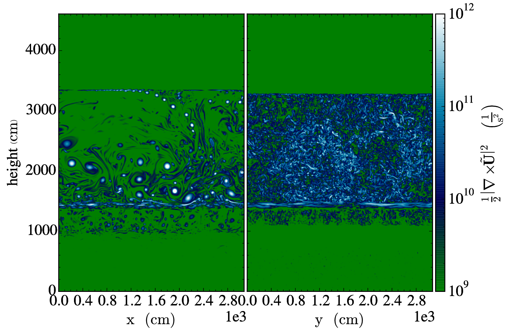
Figure 5 also shows that there is relatively more power in small scale (higher wavenumber, $k$) features for the three-dimensional simulation compared to the two-dimensional calculation. This is made more explicit by looking at a colormap plot of the enstrophy density $\eta=|\nabla\times\widetilde{{\bf{U}}}|^{2}/2$, as is shown in Figure 6, where the left (right) panel shows the two-dimensional (three-dimensional) simulation at $t=0.02$ s. The plot for the two-dimensional simulation is for the wide domain, but only half of the domain is shown to keep the same scale for both plots. For the three-dimensional simulation, the plot shows a slice through the center of the domain. The two-dimensional simulation plot appears to be dominated by moderate-sized vortices throughout the domain, while in three dimensions, we see structure on a much wider range of scales. This is similar to the results seen in comparisons of two- and three-dimensional simulations of novae (Kercek et al., 1998, 1999), although our two-dimensional results do not show as severe of a dominance of vortices as reported there.

The panels of Figure 6 also show that in two-dimensional flow the convective motions penetrate deeper into the underlying neutron star than in the three-dimensional case. This can have implications for the amount of metal-rich material that can be dredged up into the atmosphere, potentially polluting the photosphere and adjusting the opacity. We leave these details for a future paper.

Accurate analysis of the convection during a thermonuclear runaway is challenging. Most convective analysis in the literature are focused on stellar convection, which reaches a steady-state. In that case, one can drop the time derivative in the energy equation and simply compare the balance of energy fluxes. A thermonuclear runaway is far from steady state. One can assume things are in a quasi-steady state over a somewhat short timescale and perform a RANS-like averaging of the energy balance, but it is not a priori clear the exact duration of this averaging timescale. Our data dumps are roughly once every eddy turnover time, which would likely not give good enough statistics for this approach. Instead, we have, as in Malone et al. (2011, 2014), focused on the adiabatic excess, $\Delta\nabla$:

$$\Delta\nabla=\nabla-\nabla_{s};\quad\nabla\equiv\frac{d\ln T/dr}{d\ln P/dr},$$ (3)

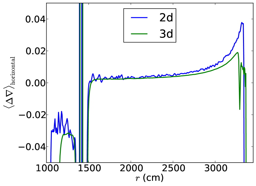
where the subscript $s$ indicates the profile along an adiabat. Figure 7 shows the horizontal average of $\Delta\nabla$ as a function of radius for both two- and three-dimensional simulations at $t=0.02$ s. This view of the convective region confirms that the extent of the convective overshoot region is less in three dimensions than in two dimensions, as was seen in the comparison of Figure 6; in this snapshot, the average overshoot region in two dimensions is roughly 50% larger than that of the three-dimensional simulation. Furthermore, the upper boundary in the two simulations is a bit different. The two dimensional simulation has a stronger degree of superadiabaticity, implying the thermal gradient is steeper than that of an adiabat. The three-dimensional simulation also appears to have, on average, a convectively stabilizing gradient around $r=3300$ cm where the adiabatic excess becomes negative before a small overshoot region extends the convection to nearly the same distance as in the two-dimensional case.

4 Discussion and Conclusions

We described the first three-dimensional models of convective burning in an XRB. While the peak temperature and Mach number behave qualitatively the same as our two-dimensional calculations, the structure of the convective velocity field differs substantially, both in the global appearance and in the turbulent statistics. This is illustrated well by the difference in appearance of the enstrophy density, which in three dimensions shows the typical cascade to small scales. Since convective mixing is expected to distribute the synthesized nuclei throughout the atmosphere, potentially bringing some to the photosphere, modeling the convection accurately is important. Based on the differences seen between the two-dimensional and three-dimensional flows, this suggests that three-dimensional models should be the focus of our future simulation efforts.

The calculations presented here pave the way for a more detailed study of convective burning in XRBs. We plan to do a more thorough analysis of the convective flow patterns in both two and three dimensions in the future paper by including tracer particles in the flow. The tracers will help visualize the trajectory of the flow, and to build a statistical analysis of the transport during a thermonuclear runaway. The wide three-dimensional simulation used 2.8 M CPU-hours on the OLCF titan system (running with 768 MPI tasks and 16 threads per task). While MAESTRO can use AMR, in these simulations we would refine the entire convective region, so the cost savings would be small. Modifying the simulation to advect and store tracer particle information should increase the computational cost by only a few percent.

Our future calculations will push for increased realism of the reaction network. As detailed in Malone et al. (2014), the approximate network used here reasonably captures the overall energy release, but we plan to both improve the nuclear reaction network with a more clever selection of isotopes for an approximate network, and to investigate using larger networks whose integration can be accelerated using highly parallel hardware accelerators, such as GPUs or Intel Xeon Phi processors.

Thus far, we have only explored a single initial model, constructed with a simple parameterization. The real state of the accreted layer can vary, and there are two potential changes worth exploring. First, we extend the isentropic layer all the way to the surface of the model, but accretion would likely cause heating at the top of the atmosphere, which could truncate the convection region before the surface. This may prevent the convective plumes from reaching the steep density gradient at the very top of the atmosphere. Second, our base density is on the higher end of likely models. We should explore lower density models as well. The burning in that case would not be as vigorous, but our timestep should increase as the convective velocity decreases, making these simulations feasible. An initial study of the initial model variations can be done in two dimensions, and then selected models can be run in three dimensions as needed.

We also plan to push our calculations to larger scales. For the near future, however, these sort of calculations will be limited to convection-in-a-box studies. Capturing the range of length scales necessary to follow a laterally propagating burning front, while resolving the energy-generation region, is not currently possible. The complementary approach to ours are the calculations by Cavecchi et al. (2012), which used wide-aspect ratio zones and did not perform hydrodynamics in the vertical direction. Ultimately these two methods can inform one-another to build a picture of nucleosynthesis and dynamics of the burning front in XRBs.

Appendix A Godunov Integration Details

Here we describe the details of the second-order Godunov integration schemes used to predict face and time-centered quantities in various steps of the algorithm. In our overall algorithm, there are three variations that share most of the same discretizations, with small differences that will be described below. In summary,

• Case 1: Construction of the advective velocities

  In Steps 3 and 7 of the algorithm flowchart in Nonaka et al. (2010), we compute face and time-centered normal velocities (i.e., we only compute $u$ at $x$-faces, $v$ at $y$-faces, etc.), $\mathbf{U}^{\mathrm{ADV},\star}$, given ${\bf{U}}^{n}$ and an associated source term, $\mathcal{S}_{{\bf{U}}}$.

• Case 2: Construction of the final velocity edge states

  In Step 11 of the MAESTRO flowchart, we compute face and time-centered velocities, ${\bf{U}}^{n+\mathchoice{\kern 0.0pt\raise 1.50694pt\hbox{\sevenrm1}\kern-1.04996pt/\kern-1.04996pt\lower 0.75346pt\hbox{\sevenrm2}}{\kern 0.0pt\raise 1.50694pt\hbox{\sevenrm1}\kern-1.04996pt/\kern-1.04996pt\lower 0.75346pt\hbox{\sevenrm2}}{\kern 0.0pt\raise 1.50694pt\hbox{\fiverm1}\kern-1.39998pt/\kern-1.04996pt\lower 0.75346pt\hbox{\fiverm2}}{1\!/2}}$, given ${\bf{U}}^{n}$ and an associated source term, $\mathcal{S}_{{\bf{U}}}$. This case is different from Case 1 in that we leverage the availability of the projected velocity field, $\widetilde{\mathbf{U}}^{\mathrm{ADV}}$, during the characteristic tracing and upwinding steps. Also, at each face we need to compute all components of velocity, rather than just the normal components.

• Case 3: Construction of the scalar edge states

  In Steps 4 and 8 of the MAESTRO flowchart, we compute face and time-centered scalars, $(\rho X_{k},\rho h)^{n+\mathchoice{\kern 0.0pt\raise 1.50694pt\hbox{\sevenrm1}\kern-1.04996pt/\kern-1.04996pt\lower 0.75346pt\hbox{\sevenrm2}}{\kern 0.0pt\raise 1.50694pt\hbox{\sevenrm1}\kern-1.04996pt/\kern-1.04996pt\lower 0.75346pt\hbox{\sevenrm2}}{\kern 0.0pt\raise 1.50694pt\hbox{\fiverm1}\kern-1.39998pt/\kern-1.04996pt\lower 0.75346pt\hbox{\fiverm2}}{1\!/2},(l)}$, given $(\rho X_{k},\rho h)^{n}$ and the associated source terms, $\mathcal{S}_{\rho X_{k}},\mathcal{S}_{\rho h}$. This is different from Case 2 in that the evolution equations for the scalars are in conservative form rather than advective form.

Our Godunov integration strategy is based on the piecewise parabolic method (PPM) of Colella & Woodward (1984). We modify this algorithm to account for the fact that (i) our underlying velocity field is spatially-varying, (ii) we require a multidimensionally unsplit discretization, (iii) we have governing equations in both advective and conservative form,

$$\frac{\partial q}{\partial t}=-{\bf{U}}\cdot\nabla q+\mathcal{S}_{q};\quad q=u,v,~{}\text{or}~{}w,$$ (A1)

$$\frac{\partial q}{\partial t}=-\nabla\cdot({\bf{U}}q)+\mathcal{S}_{q};\quad q=\rho X_{k}~{}\text{or}~{}\rho h.$$ (A2)

Which form is used for the scalars, $(\rho X_{k})$ and $(\rho h)$, is determined at runtime based on how we chose to bring these states to the interface. MAESTRO offers several possibilities, e.g., bringing $(\rho X_{k})$ to the interface as a single quantity, bring $\rho^{\prime}$ and $X_{k}$ to the interface separately, or bringing $\rho$ and $X_{k}$ to the interface separately. Even more variation is allowed for $(\rho h)$, where we can use $T$ instead of $h$ for the interface prediction. We document both forms of interface reconstruction here. The full list of possible states is provided in the MAESTRO User’s Guide. For the present simulations, we predict $\rho$ and $X_{k}$ separately for form $(\rho X_{k})$ on interfaces, and $T$ is predicted and converted to $h$ on the interface via the equation of state.

For all cases, the idea is to use the original PPM algorithm is to predict preliminary face and time-centered states, $q^{\rm 1D}$, using a one-dimensional advection equation for each direction $d$,

$$\frac{\partial q}{\partial t}=-U_{d}\frac{\partial q}{\partial x_{d}},$$ (A3)

and then use these states in a multidimensionally unsplit discretization of the full equations of motion based on the ideas in Colella (1990); Saltzman (1994) to compute updated face and time-centered states. We now provide the details of our method.

A.1 Case 1

Here we compute face and time-centered estimates of the normal velocity. We begin by computing preliminary face and time-centered estimates of all velocity components at every face. Here, $q$ will represent an arbitrary component of velocity ($u,v$, or $w$). The following developments are for the $x$-direction and we omit the $j,k$ subscripts for ease of exposition; the equations for the $y$ and $z$-directions are analogous. The first step is to construct a parabolic profile, $q(x)$, in each zone following the methodology discussed in Colella & Woodward (1984).

$$q(x)=q_{i,-}+\xi(x)(q_{i,+}-q_{i,-}+q_{6,i}(1-\xi(x)))$$ (A4)

where $q_{i,-}$ and $q_{i,+}$ are the limited edge values of the parabola and $q_{6,i}=6q_{i}-3(q_{i,-}+q_{i,+})$ is related to the curvature. The quantity $\xi(x)$ converts $x$ into the fraction of the zone from the left edge.

The parabolic profiles are then integrated along characteristics to get the average value swept over the high and low faces over the time step. By defining

$$\sigma=|u_{i}|\frac{\Delta t}{\Delta x},$$ (A5)

we obtain:

$$(q_{L}^{\rm 1D})_{i+\mathchoice{\kern 0.0pt\raise 1.50694pt\hbox{\sevenrm1}\kern-1.04996pt/\kern-1.04996pt\lower 0.75346pt\hbox{\sevenrm2}}{\kern 0.0pt\raise 1.50694pt\hbox{\sevenrm1}\kern-1.04996pt/\kern-1.04996pt\lower 0.75346pt\hbox{\sevenrm2}}{\kern 0.0pt\raise 1.50694pt\hbox{\fiverm1}\kern-1.39998pt/\kern-1.04996pt\lower 0.75346pt\hbox{\fiverm2}}{1\!/2}} = \begin{cases}q_{i,+}-\frac{\sigma}{2}\left[(q_{i,+}-q_{i,-})-\left(1-\frac{2}{3}\sigma\right)q_{6,i}\right],&u_{i}>0\\ q_{i},&\rm{otherwise}\end{cases},$$ (A6)

$$(q_{R}^{\rm 1D})_{i-\mathchoice{\kern 0.0pt\raise 1.50694pt\hbox{\sevenrm1}\kern-1.04996pt/\kern-1.04996pt\lower 0.75346pt\hbox{\sevenrm2}}{\kern 0.0pt\raise 1.50694pt\hbox{\sevenrm1}\kern-1.04996pt/\kern-1.04996pt\lower 0.75346pt\hbox{\sevenrm2}}{\kern 0.0pt\raise 1.50694pt\hbox{\fiverm1}\kern-1.39998pt/\kern-1.04996pt\lower 0.75346pt\hbox{\fiverm2}}{1\!/2}} = \begin{cases}q_{i,-}+\frac{\sigma}{2}\left[(q_{i,+}-q_{i,-})+\left(1-\frac{2}{3}\sigma\right)q_{6,i}\right],&u_{i}<0\\ q_{i},&\rm{otherwise}\end{cases}.$$ (A7)

Then, for the normal velocity components, we solve a Riemann problem to obtain the preliminary state at the face,

$$u_{i+\mathchoice{\kern 0.0pt\raise 1.50694pt\hbox{\sevenrm1}\kern-1.04996pt/\kern-1.04996pt\lower 0.75346pt\hbox{\sevenrm2}}{\kern 0.0pt\raise 1.50694pt\hbox{\sevenrm1}\kern-1.04996pt/\kern-1.04996pt\lower 0.75346pt\hbox{\sevenrm2}}{\kern 0.0pt\raise 1.50694pt\hbox{\fiverm1}\kern-1.39998pt/\kern-1.04996pt\lower 0.75346pt\hbox{\fiverm2}}{1\!/2}}^{\rm 1D}=\mathcal{R}\left((u_{L}^{\rm 1D})_{i+\mathchoice{\kern 0.0pt\raise 1.50694pt\hbox{\sevenrm1}\kern-1.04996pt/\kern-1.04996pt\lower 0.75346pt\hbox{\sevenrm2}}{\kern 0.0pt\raise 1.50694pt\hbox{\sevenrm1}\kern-1.04996pt/\kern-1.04996pt\lower 0.75346pt\hbox{\sevenrm2}}{\kern 0.0pt\raise 1.50694pt\hbox{\fiverm1}\kern-1.39998pt/\kern-1.04996pt\lower 0.75346pt\hbox{\fiverm2}}{1\!/2}},(u_{R}^{\rm 1D})_{i+\mathchoice{\kern 0.0pt\raise 1.50694pt\hbox{\sevenrm1}\kern-1.04996pt/\kern-1.04996pt\lower 0.75346pt\hbox{\sevenrm2}}{\kern 0.0pt\raise 1.50694pt\hbox{\sevenrm1}\kern-1.04996pt/\kern-1.04996pt\lower 0.75346pt\hbox{\sevenrm2}}{\kern 0.0pt\raise 1.50694pt\hbox{\fiverm1}\kern-1.39998pt/\kern-1.04996pt\lower 0.75346pt\hbox{\fiverm2}}{1\!/2}}\right)=\begin{cases}0,&(u_{L}^{\rm 1D})_{i+\mathchoice{\kern 0.0pt\raise 1.50694pt\hbox{\sevenrm1}\kern-1.04996pt/\kern-1.04996pt\lower 0.75346pt\hbox{\sevenrm2}}{\kern 0.0pt\raise 1.50694pt\hbox{\sevenrm1}\kern-1.04996pt/\kern-1.04996pt\lower 0.75346pt\hbox{\sevenrm2}}{\kern 0.0pt\raise 1.50694pt\hbox{\fiverm1}\kern-1.39998pt/\kern-1.04996pt\lower 0.75346pt\hbox{\fiverm2}}{1\!/2}}\leq 0~{}~{}{\rm AND}~{}~{}(u_{R}^{\rm 1D})_{i+\mathchoice{\kern 0.0pt\raise 1.50694pt\hbox{\sevenrm1}\kern-1.04996pt/\kern-1.04996pt\lower 0.75346pt\hbox{\sevenrm2}}{\kern 0.0pt\raise 1.50694pt\hbox{\sevenrm1}\kern-1.04996pt/\kern-1.04996pt\lower 0.75346pt\hbox{\sevenrm2}}{\kern 0.0pt\raise 1.50694pt\hbox{\fiverm1}\kern-1.39998pt/\kern-1.04996pt\lower 0.75346pt\hbox{\fiverm2}}{1\!/2}}\geq 0\\ (u_{L}^{\rm 1D})_{i+\mathchoice{\kern 0.0pt\raise 1.50694pt\hbox{\sevenrm1}\kern-1.04996pt/\kern-1.04996pt\lower 0.75346pt\hbox{\sevenrm2}}{\kern 0.0pt\raise 1.50694pt\hbox{\sevenrm1}\kern-1.04996pt/\kern-1.04996pt\lower 0.75346pt\hbox{\sevenrm2}}{\kern 0.0pt\raise 1.50694pt\hbox{\fiverm1}\kern-1.39998pt/\kern-1.04996pt\lower 0.75346pt\hbox{\fiverm2}}{1\!/2}},&(u_{L}^{\rm 1D})_{i+\mathchoice{\kern 0.0pt\raise 1.50694pt\hbox{\sevenrm1}\kern-1.04996pt/\kern-1.04996pt\lower 0.75346pt\hbox{\sevenrm2}}{\kern 0.0pt\raise 1.50694pt\hbox{\sevenrm1}\kern-1.04996pt/\kern-1.04996pt\lower 0.75346pt\hbox{\sevenrm2}}{\kern 0.0pt\raise 1.50694pt\hbox{\fiverm1}\kern-1.39998pt/\kern-1.04996pt\lower 0.75346pt\hbox{\fiverm2}}{1\!/2}}+(u_{R}^{\rm 1D})_{i+\mathchoice{\kern 0.0pt\raise 1.50694pt\hbox{\sevenrm1}\kern-1.04996pt/\kern-1.04996pt\lower 0.75346pt\hbox{\sevenrm2}}{\kern 0.0pt\raise 1.50694pt\hbox{\sevenrm1}\kern-1.04996pt/\kern-1.04996pt\lower 0.75346pt\hbox{\sevenrm2}}{\kern 0.0pt\raise 1.50694pt\hbox{\fiverm1}\kern-1.39998pt/\kern-1.04996pt\lower 0.75346pt\hbox{\fiverm2}}{1\!/2}}>0\\ (u_{R}^{\rm 1D})_{i+\mathchoice{\kern 0.0pt\raise 1.50694pt\hbox{\sevenrm1}\kern-1.04996pt/\kern-1.04996pt\lower 0.75346pt\hbox{\sevenrm2}}{\kern 0.0pt\raise 1.50694pt\hbox{\sevenrm1}\kern-1.04996pt/\kern-1.04996pt\lower 0.75346pt\hbox{\sevenrm2}}{\kern 0.0pt\raise 1.50694pt\hbox{\fiverm1}\kern-1.39998pt/\kern-1.04996pt\lower 0.75346pt\hbox{\fiverm2}}{1\!/2}},&(u_{L}^{\rm 1D})_{i+\mathchoice{\kern 0.0pt\raise 1.50694pt\hbox{\sevenrm1}\kern-1.04996pt/\kern-1.04996pt\lower 0.75346pt\hbox{\sevenrm2}}{\kern 0.0pt\raise 1.50694pt\hbox{\sevenrm1}\kern-1.04996pt/\kern-1.04996pt\lower 0.75346pt\hbox{\sevenrm2}}{\kern 0.0pt\raise 1.50694pt\hbox{\fiverm1}\kern-1.39998pt/\kern-1.04996pt\lower 0.75346pt\hbox{\fiverm2}}{1\!/2}}+(u_{R}^{\rm 1D})_{i+\mathchoice{\kern 0.0pt\raise 1.50694pt\hbox{\sevenrm1}\kern-1.04996pt/\kern-1.04996pt\lower 0.75346pt\hbox{\sevenrm2}}{\kern 0.0pt\raise 1.50694pt\hbox{\sevenrm1}\kern-1.04996pt/\kern-1.04996pt\lower 0.75346pt\hbox{\sevenrm2}}{\kern 0.0pt\raise 1.50694pt\hbox{\fiverm1}\kern-1.39998pt/\kern-1.04996pt\lower 0.75346pt\hbox{\fiverm2}}{1\!/2}}<0\end{cases}.$$ (A8)

Next, we obtain the preliminary face and time-centered transverse velocities using upwinding,

$$v_{i+\mathchoice{\kern 0.0pt\raise 1.50694pt\hbox{\sevenrm1}\kern-1.04996pt/\kern-1.04996pt\lower 0.75346pt\hbox{\sevenrm2}}{\kern 0.0pt\raise 1.50694pt\hbox{\sevenrm1}\kern-1.04996pt/\kern-1.04996pt\lower 0.75346pt\hbox{\sevenrm2}}{\kern 0.0pt\raise 1.50694pt\hbox{\fiverm1}\kern-1.39998pt/\kern-1.04996pt\lower 0.75346pt\hbox{\fiverm2}}{1\!/2}}^{1D}=\mathcal{U}\left((v_{L}^{\rm 1D})_{i+\mathchoice{\kern 0.0pt\raise 1.50694pt\hbox{\sevenrm1}\kern-1.04996pt/\kern-1.04996pt\lower 0.75346pt\hbox{\sevenrm2}}{\kern 0.0pt\raise 1.50694pt\hbox{\sevenrm1}\kern-1.04996pt/\kern-1.04996pt\lower 0.75346pt\hbox{\sevenrm2}}{\kern 0.0pt\raise 1.50694pt\hbox{\fiverm1}\kern-1.39998pt/\kern-1.04996pt\lower 0.75346pt\hbox{\fiverm2}}{1\!/2}},(v_{R}^{\rm 1D})_{i+\mathchoice{\kern 0.0pt\raise 1.50694pt\hbox{\sevenrm1}\kern-1.04996pt/\kern-1.04996pt\lower 0.75346pt\hbox{\sevenrm2}}{\kern 0.0pt\raise 1.50694pt\hbox{\sevenrm1}\kern-1.04996pt/\kern-1.04996pt\lower 0.75346pt\hbox{\sevenrm2}}{\kern 0.0pt\raise 1.50694pt\hbox{\fiverm1}\kern-1.39998pt/\kern-1.04996pt\lower 0.75346pt\hbox{\fiverm2}}{1\!/2}},u_{i+\mathchoice{\kern 0.0pt\raise 1.50694pt\hbox{\sevenrm1}\kern-1.04996pt/\kern-1.04996pt\lower 0.75346pt\hbox{\sevenrm2}}{\kern 0.0pt\raise 1.50694pt\hbox{\sevenrm1}\kern-1.04996pt/\kern-1.04996pt\lower 0.75346pt\hbox{\sevenrm2}}{\kern 0.0pt\raise 1.50694pt\hbox{\fiverm1}\kern-1.39998pt/\kern-1.04996pt\lower 0.75346pt\hbox{\fiverm2}}{1\!/2}}^{\rm 1D}\right)=\begin{cases}(v_{L})_{i+\mathchoice{\kern 0.0pt\raise 1.50694pt\hbox{\sevenrm1}\kern-1.04996pt/\kern-1.04996pt\lower 0.75346pt\hbox{\sevenrm2}}{\kern 0.0pt\raise 1.50694pt\hbox{\sevenrm1}\kern-1.04996pt/\kern-1.04996pt\lower 0.75346pt\hbox{\sevenrm2}}{\kern 0.0pt\raise 1.50694pt\hbox{\fiverm1}\kern-1.39998pt/\kern-1.04996pt\lower 0.75346pt\hbox{\fiverm2}}{1\!/2}}^{\rm 1D},&u_{i+\mathchoice{\kern 0.0pt\raise 1.50694pt\hbox{\sevenrm1}\kern-1.04996pt/\kern-1.04996pt\lower 0.75346pt\hbox{\sevenrm2}}{\kern 0.0pt\raise 1.50694pt\hbox{\sevenrm1}\kern-1.04996pt/\kern-1.04996pt\lower 0.75346pt\hbox{\sevenrm2}}{\kern 0.0pt\raise 1.50694pt\hbox{\fiverm1}\kern-1.39998pt/\kern-1.04996pt\lower 0.75346pt\hbox{\fiverm2}}{1\!/2}}^{\rm 1D}>0\\ (v_{R})_{i+\mathchoice{\kern 0.0pt\raise 1.50694pt\hbox{\sevenrm1}\kern-1.04996pt/\kern-1.04996pt\lower 0.75346pt\hbox{\sevenrm2}}{\kern 0.0pt\raise 1.50694pt\hbox{\sevenrm1}\kern-1.04996pt/\kern-1.04996pt\lower 0.75346pt\hbox{\sevenrm2}}{\kern 0.0pt\raise 1.50694pt\hbox{\fiverm1}\kern-1.39998pt/\kern-1.04996pt\lower 0.75346pt\hbox{\fiverm2}}{1\!/2}}^{\rm 1D},&u_{i+\mathchoice{\kern 0.0pt\raise 1.50694pt\hbox{\sevenrm1}\kern-1.04996pt/\kern-1.04996pt\lower 0.75346pt\hbox{\sevenrm2}}{\kern 0.0pt\raise 1.50694pt\hbox{\sevenrm1}\kern-1.04996pt/\kern-1.04996pt\lower 0.75346pt\hbox{\sevenrm2}}{\kern 0.0pt\raise 1.50694pt\hbox{\fiverm1}\kern-1.39998pt/\kern-1.04996pt\lower 0.75346pt\hbox{\fiverm2}}{1\!/2}}^{\rm 1D}<0\end{cases}.$$ (A9)

We now have $u^{\rm 1D}$ and $v^{\rm 1D}$ at each face. The next step is compute updated face and time-centered normal velocities by accounting for the transverse derivative and source terms we have ignored so far. In two dimensions, first compute $(u_{L})_{i+\mathchoice{\kern 0.0pt\raise 1.50694pt\hbox{\sevenrm1}\kern-1.04996pt/\kern-1.04996pt\lower 0.75346pt\hbox{\sevenrm2}}{\kern 0.0pt\raise 1.50694pt\hbox{\sevenrm1}\kern-1.04996pt/\kern-1.04996pt\lower 0.75346pt\hbox{\sevenrm2}}{\kern 0.0pt\raise 1.50694pt\hbox{\fiverm1}\kern-1.39998pt/\kern-1.04996pt\lower 0.75346pt\hbox{\fiverm2}}{1\!/2},j}$ and $(u_{R})_{i+\mathchoice{\kern 0.0pt\raise 1.50694pt\hbox{\sevenrm1}\kern-1.04996pt/\kern-1.04996pt\lower 0.75346pt\hbox{\sevenrm2}}{\kern 0.0pt\raise 1.50694pt\hbox{\sevenrm1}\kern-1.04996pt/\kern-1.04996pt\lower 0.75346pt\hbox{\sevenrm2}}{\kern 0.0pt\raise 1.50694pt\hbox{\fiverm1}\kern-1.39998pt/\kern-1.04996pt\lower 0.75346pt\hbox{\fiverm2}}{1\!/2},j}$ using, e.g.,

$$(u_{L})_{i+\mathchoice{\kern 0.0pt\raise 1.50694pt\hbox{\sevenrm1}\kern-1.04996pt/\kern-1.04996pt\lower 0.75346pt\hbox{\sevenrm2}}{\kern 0.0pt\raise 1.50694pt\hbox{\sevenrm1}\kern-1.04996pt/\kern-1.04996pt\lower 0.75346pt\hbox{\sevenrm2}}{\kern 0.0pt\raise 1.50694pt\hbox{\fiverm1}\kern-1.39998pt/\kern-1.04996pt\lower 0.75346pt\hbox{\fiverm2}}{1\!/2},j}=(u_{L}^{\rm 1D})_{i+\mathchoice{\kern 0.0pt\raise 1.50694pt\hbox{\sevenrm1}\kern-1.04996pt/\kern-1.04996pt\lower 0.75346pt\hbox{\sevenrm2}}{\kern 0.0pt\raise 1.50694pt\hbox{\sevenrm1}\kern-1.04996pt/\kern-1.04996pt\lower 0.75346pt\hbox{\sevenrm2}}{\kern 0.0pt\raise 1.50694pt\hbox{\fiverm1}\kern-1.39998pt/\kern-1.04996pt\lower 0.75346pt\hbox{\fiverm2}}{1\!/2},j}-\frac{\Delta t}{2}\left(\frac{v_{i,j+\mathchoice{\kern 0.0pt\raise 1.50694pt\hbox{\sevenrm1}\kern-1.04996pt/\kern-1.04996pt\lower 0.75346pt\hbox{\sevenrm2}}{\kern 0.0pt\raise 1.50694pt\hbox{\sevenrm1}\kern-1.04996pt/\kern-1.04996pt\lower 0.75346pt\hbox{\sevenrm2}}{\kern 0.0pt\raise 1.50694pt\hbox{\fiverm1}\kern-1.39998pt/\kern-1.04996pt\lower 0.75346pt\hbox{\fiverm2}}{1\!/2}}^{\rm 1D}+v_{i,j-\mathchoice{\kern 0.0pt\raise 1.50694pt\hbox{\sevenrm1}\kern-1.04996pt/\kern-1.04996pt\lower 0.75346pt\hbox{\sevenrm2}}{\kern 0.0pt\raise 1.50694pt\hbox{\sevenrm1}\kern-1.04996pt/\kern-1.04996pt\lower 0.75346pt\hbox{\sevenrm2}}{\kern 0.0pt\raise 1.50694pt\hbox{\fiverm1}\kern-1.39998pt/\kern-1.04996pt\lower 0.75346pt\hbox{\fiverm2}}{1\!/2}}^{\rm 1D}}{2}\right)\left(\frac{u^{\rm 1D}_{i,j+\mathchoice{\kern 0.0pt\raise 1.50694pt\hbox{\sevenrm1}\kern-1.04996pt/\kern-1.04996pt\lower 0.75346pt\hbox{\sevenrm2}}{\kern 0.0pt\raise 1.50694pt\hbox{\sevenrm1}\kern-1.04996pt/\kern-1.04996pt\lower 0.75346pt\hbox{\sevenrm2}}{\kern 0.0pt\raise 1.50694pt\hbox{\fiverm1}\kern-1.39998pt/\kern-1.04996pt\lower 0.75346pt\hbox{\fiverm2}}{1\!/2}}-u^{\rm 1D}_{i,j-\mathchoice{\kern 0.0pt\raise 1.50694pt\hbox{\sevenrm1}\kern-1.04996pt/\kern-1.04996pt\lower 0.75346pt\hbox{\sevenrm2}}{\kern 0.0pt\raise 1.50694pt\hbox{\sevenrm1}\kern-1.04996pt/\kern-1.04996pt\lower 0.75346pt\hbox{\sevenrm2}}{\kern 0.0pt\raise 1.50694pt\hbox{\fiverm1}\kern-1.39998pt/\kern-1.04996pt\lower 0.75346pt\hbox{\fiverm2}}{1\!/2}}}{\Delta y}\right)+\frac{\Delta t}{2}(\mathcal{S}_{u})_{{\bf i}},$$ (A10)

followed by a Riemann solver to obtain the final face and time-centered state,

$$u_{i+\mathchoice{\kern 0.0pt\raise 1.50694pt\hbox{\sevenrm1}\kern-1.04996pt/\kern-1.04996pt\lower 0.75346pt\hbox{\sevenrm2}}{\kern 0.0pt\raise 1.50694pt\hbox{\sevenrm1}\kern-1.04996pt/\kern-1.04996pt\lower 0.75346pt\hbox{\sevenrm2}}{\kern 0.0pt\raise 1.50694pt\hbox{\fiverm1}\kern-1.39998pt/\kern-1.04996pt\lower 0.75346pt\hbox{\fiverm2}}{1\!/2},j}^{\rm ADV,\star}=\mathcal{R}\left((u_{L})_{i+\mathchoice{\kern 0.0pt\raise 1.50694pt\hbox{\sevenrm1}\kern-1.04996pt/\kern-1.04996pt\lower 0.75346pt\hbox{\sevenrm2}}{\kern 0.0pt\raise 1.50694pt\hbox{\sevenrm1}\kern-1.04996pt/\kern-1.04996pt\lower 0.75346pt\hbox{\sevenrm2}}{\kern 0.0pt\raise 1.50694pt\hbox{\fiverm1}\kern-1.39998pt/\kern-1.04996pt\lower 0.75346pt\hbox{\fiverm2}}{1\!/2},j},(u_{R})_{i+\mathchoice{\kern 0.0pt\raise 1.50694pt\hbox{\sevenrm1}\kern-1.04996pt/\kern-1.04996pt\lower 0.75346pt\hbox{\sevenrm2}}{\kern 0.0pt\raise 1.50694pt\hbox{\sevenrm1}\kern-1.04996pt/\kern-1.04996pt\lower 0.75346pt\hbox{\sevenrm2}}{\kern 0.0pt\raise 1.50694pt\hbox{\fiverm1}\kern-1.39998pt/\kern-1.04996pt\lower 0.75346pt\hbox{\fiverm2}}{1\!/2},j}\right).$$ (A11)

In three dimensions, instead of Equation (A10) we use

$$(u_{L})_{i+\mathchoice{\kern 0.0pt\raise 1.50694pt\hbox{\sevenrm1}\kern-1.04996pt/\kern-1.04996pt\lower 0.75346pt\hbox{\sevenrm2}}{\kern 0.0pt\raise 1.50694pt\hbox{\sevenrm1}\kern-1.04996pt/\kern-1.04996pt\lower 0.75346pt\hbox{\sevenrm2}}{\kern 0.0pt\raise 1.50694pt\hbox{\fiverm1}\kern-1.39998pt/\kern-1.04996pt\lower 0.75346pt\hbox{\fiverm2}}{1\!/2},j,k} = (u_{L}^{\rm 1D})_{i+\mathchoice{\kern 0.0pt\raise 1.50694pt\hbox{\sevenrm1}\kern-1.04996pt/\kern-1.04996pt\lower 0.75346pt\hbox{\sevenrm2}}{\kern 0.0pt\raise 1.50694pt\hbox{\sevenrm1}\kern-1.04996pt/\kern-1.04996pt\lower 0.75346pt\hbox{\sevenrm2}}{\kern 0.0pt\raise 1.50694pt\hbox{\fiverm1}\kern-1.39998pt/\kern-1.04996pt\lower 0.75346pt\hbox{\fiverm2}}{1\!/2},j,k}-\frac{\Delta t}{2}\left(\frac{v_{i,j+\mathchoice{\kern 0.0pt\raise 1.50694pt\hbox{\sevenrm1}\kern-1.04996pt/\kern-1.04996pt\lower 0.75346pt\hbox{\sevenrm2}}{\kern 0.0pt\raise 1.50694pt\hbox{\sevenrm1}\kern-1.04996pt/\kern-1.04996pt\lower 0.75346pt\hbox{\sevenrm2}}{\kern 0.0pt\raise 1.50694pt\hbox{\fiverm1}\kern-1.39998pt/\kern-1.04996pt\lower 0.75346pt\hbox{\fiverm2}}{1\!/2},k}^{\rm 1D}+v_{i,j-\mathchoice{\kern 0.0pt\raise 1.50694pt\hbox{\sevenrm1}\kern-1.04996pt/\kern-1.04996pt\lower 0.75346pt\hbox{\sevenrm2}}{\kern 0.0pt\raise 1.50694pt\hbox{\sevenrm1}\kern-1.04996pt/\kern-1.04996pt\lower 0.75346pt\hbox{\sevenrm2}}{\kern 0.0pt\raise 1.50694pt\hbox{\fiverm1}\kern-1.39998pt/\kern-1.04996pt\lower 0.75346pt\hbox{\fiverm2}}{1\!/2},k}^{\rm 1D}}{2}\right)\left(\frac{u^{y|z}_{i,j+\mathchoice{\kern 0.0pt\raise 1.50694pt\hbox{\sevenrm1}\kern-1.04996pt/\kern-1.04996pt\lower 0.75346pt\hbox{\sevenrm2}}{\kern 0.0pt\raise 1.50694pt\hbox{\sevenrm1}\kern-1.04996pt/\kern-1.04996pt\lower 0.75346pt\hbox{\sevenrm2}}{\kern 0.0pt\raise 1.50694pt\hbox{\fiverm1}\kern-1.39998pt/\kern-1.04996pt\lower 0.75346pt\hbox{\fiverm2}}{1\!/2},k}-u^{y|z}_{i,j-\mathchoice{\kern 0.0pt\raise 1.50694pt\hbox{\sevenrm1}\kern-1.04996pt/\kern-1.04996pt\lower 0.75346pt\hbox{\sevenrm2}}{\kern 0.0pt\raise 1.50694pt\hbox{\sevenrm1}\kern-1.04996pt/\kern-1.04996pt\lower 0.75346pt\hbox{\sevenrm2}}{\kern 0.0pt\raise 1.50694pt\hbox{\fiverm1}\kern-1.39998pt/\kern-1.04996pt\lower 0.75346pt\hbox{\fiverm2}}{1\!/2},k}}{\Delta y}\right)$$

$$\hskip 65.04256pt-\frac{\Delta t}{2}\left(\frac{w_{i,j,k+\mathchoice{\kern 0.0pt\raise 1.50694pt\hbox{\sevenrm1}\kern-1.04996pt/\kern-1.04996pt\lower 0.75346pt\hbox{\sevenrm2}}{\kern 0.0pt\raise 1.50694pt\hbox{\sevenrm1}\kern-1.04996pt/\kern-1.04996pt\lower 0.75346pt\hbox{\sevenrm2}}{\kern 0.0pt\raise 1.50694pt\hbox{\fiverm1}\kern-1.39998pt/\kern-1.04996pt\lower 0.75346pt\hbox{\fiverm2}}{1\!/2}}^{\rm 1D}+v_{i,j,k-\mathchoice{\kern 0.0pt\raise 1.50694pt\hbox{\sevenrm1}\kern-1.04996pt/\kern-1.04996pt\lower 0.75346pt\hbox{\sevenrm2}}{\kern 0.0pt\raise 1.50694pt\hbox{\sevenrm1}\kern-1.04996pt/\kern-1.04996pt\lower 0.75346pt\hbox{\sevenrm2}}{\kern 0.0pt\raise 1.50694pt\hbox{\fiverm1}\kern-1.39998pt/\kern-1.04996pt\lower 0.75346pt\hbox{\fiverm2}}{1\!/2}}^{\rm 1D}}{2}\right)\left(\frac{u^{z|y}_{i,j,k+\mathchoice{\kern 0.0pt\raise 1.50694pt\hbox{\sevenrm1}\kern-1.04996pt/\kern-1.04996pt\lower 0.75346pt\hbox{\sevenrm2}}{\kern 0.0pt\raise 1.50694pt\hbox{\sevenrm1}\kern-1.04996pt/\kern-1.04996pt\lower 0.75346pt\hbox{\sevenrm2}}{\kern 0.0pt\raise 1.50694pt\hbox{\fiverm1}\kern-1.39998pt/\kern-1.04996pt\lower 0.75346pt\hbox{\fiverm2}}{1\!/2}}-u^{z|y}_{i,j,k-\mathchoice{\kern 0.0pt\raise 1.50694pt\hbox{\sevenrm1}\kern-1.04996pt/\kern-1.04996pt\lower 0.75346pt\hbox{\sevenrm2}}{\kern 0.0pt\raise 1.50694pt\hbox{\sevenrm1}\kern-1.04996pt/\kern-1.04996pt\lower 0.75346pt\hbox{\sevenrm2}}{\kern 0.0pt\raise 1.50694pt\hbox{\fiverm1}\kern-1.39998pt/\kern-1.04996pt\lower 0.75346pt\hbox{\fiverm2}}{1\!/2}}}{\Delta z}\right)+\frac{\Delta t}{2}(\mathcal{S}_{u})_{{\bf i}},$$

where to account for transverse corner coupling, we compute the intermediate states as in Colella (1990); Saltzman (1994). For example,

$$(u_{L}^{y|z})_{i,j+\mathchoice{\kern 0.0pt\raise 1.50694pt\hbox{\sevenrm1}\kern-1.04996pt/\kern-1.04996pt\lower 0.75346pt\hbox{\sevenrm2}}{\kern 0.0pt\raise 1.50694pt\hbox{\sevenrm1}\kern-1.04996pt/\kern-1.04996pt\lower 0.75346pt\hbox{\sevenrm2}}{\kern 0.0pt\raise 1.50694pt\hbox{\fiverm1}\kern-1.39998pt/\kern-1.04996pt\lower 0.75346pt\hbox{\fiverm2}}{1\!/2},k}=(u_{L})_{i,j+\mathchoice{\kern 0.0pt\raise 1.50694pt\hbox{\sevenrm1}\kern-1.04996pt/\kern-1.04996pt\lower 0.75346pt\hbox{\sevenrm2}}{\kern 0.0pt\raise 1.50694pt\hbox{\sevenrm1}\kern-1.04996pt/\kern-1.04996pt\lower 0.75346pt\hbox{\sevenrm2}}{\kern 0.0pt\raise 1.50694pt\hbox{\fiverm1}\kern-1.39998pt/\kern-1.04996pt\lower 0.75346pt\hbox{\fiverm2}}{1\!/2},k}-\frac{\Delta t}{3}\left(\frac{w_{i,j,k+\mathchoice{\kern 0.0pt\raise 1.50694pt\hbox{\sevenrm1}\kern-1.04996pt/\kern-1.04996pt\lower 0.75346pt\hbox{\sevenrm2}}{\kern 0.0pt\raise 1.50694pt\hbox{\sevenrm1}\kern-1.04996pt/\kern-1.04996pt\lower 0.75346pt\hbox{\sevenrm2}}{\kern 0.0pt\raise 1.50694pt\hbox{\fiverm1}\kern-1.39998pt/\kern-1.04996pt\lower 0.75346pt\hbox{\fiverm2}}{1\!/2}}^{\rm 1D}+w_{i,j,k-\mathchoice{\kern 0.0pt\raise 1.50694pt\hbox{\sevenrm1}\kern-1.04996pt/\kern-1.04996pt\lower 0.75346pt\hbox{\sevenrm2}}{\kern 0.0pt\raise 1.50694pt\hbox{\sevenrm1}\kern-1.04996pt/\kern-1.04996pt\lower 0.75346pt\hbox{\sevenrm2}}{\kern 0.0pt\raise 1.50694pt\hbox{\fiverm1}\kern-1.39998pt/\kern-1.04996pt\lower 0.75346pt\hbox{\fiverm2}}{1\!/2}}^{\rm 1D}}{2}\right)\left(\frac{u_{i,j,k+\mathchoice{\kern 0.0pt\raise 1.50694pt\hbox{\sevenrm1}\kern-1.04996pt/\kern-1.04996pt\lower 0.75346pt\hbox{\sevenrm2}}{\kern 0.0pt\raise 1.50694pt\hbox{\sevenrm1}\kern-1.04996pt/\kern-1.04996pt\lower 0.75346pt\hbox{\sevenrm2}}{\kern 0.0pt\raise 1.50694pt\hbox{\fiverm1}\kern-1.39998pt/\kern-1.04996pt\lower 0.75346pt\hbox{\fiverm2}}{1\!/2}}^{\rm 1D}-u_{i,j,k-\mathchoice{\kern 0.0pt\raise 1.50694pt\hbox{\sevenrm1}\kern-1.04996pt/\kern-1.04996pt\lower 0.75346pt\hbox{\sevenrm2}}{\kern 0.0pt\raise 1.50694pt\hbox{\sevenrm1}\kern-1.04996pt/\kern-1.04996pt\lower 0.75346pt\hbox{\sevenrm2}}{\kern 0.0pt\raise 1.50694pt\hbox{\fiverm1}\kern-1.39998pt/\kern-1.04996pt\lower 0.75346pt\hbox{\fiverm2}}{1\!/2}}^{\rm 1D}}{\Delta z}\right),$$ (A13)

$$u_{i,j+\mathchoice{\kern 0.0pt\raise 1.50694pt\hbox{\sevenrm1}\kern-1.04996pt/\kern-1.04996pt\lower 0.75346pt\hbox{\sevenrm2}}{\kern 0.0pt\raise 1.50694pt\hbox{\sevenrm1}\kern-1.04996pt/\kern-1.04996pt\lower 0.75346pt\hbox{\sevenrm2}}{\kern 0.0pt\raise 1.50694pt\hbox{\fiverm1}\kern-1.39998pt/\kern-1.04996pt\lower 0.75346pt\hbox{\fiverm2}}{1\!/2},k}^{y|z}=\mathcal{U}\left((u_{L}^{y|z})_{i,j+\mathchoice{\kern 0.0pt\raise 1.50694pt\hbox{\sevenrm1}\kern-1.04996pt/\kern-1.04996pt\lower 0.75346pt\hbox{\sevenrm2}}{\kern 0.0pt\raise 1.50694pt\hbox{\sevenrm1}\kern-1.04996pt/\kern-1.04996pt\lower 0.75346pt\hbox{\sevenrm2}}{\kern 0.0pt\raise 1.50694pt\hbox{\fiverm1}\kern-1.39998pt/\kern-1.04996pt\lower 0.75346pt\hbox{\fiverm2}}{1\!/2},k},(u_{R}^{y|z})_{i,j+\mathchoice{\kern 0.0pt\raise 1.50694pt\hbox{\sevenrm1}\kern-1.04996pt/\kern-1.04996pt\lower 0.75346pt\hbox{\sevenrm2}}{\kern 0.0pt\raise 1.50694pt\hbox{\sevenrm1}\kern-1.04996pt/\kern-1.04996pt\lower 0.75346pt\hbox{\sevenrm2}}{\kern 0.0pt\raise 1.50694pt\hbox{\fiverm1}\kern-1.39998pt/\kern-1.04996pt\lower 0.75346pt\hbox{\fiverm2}}{1\!/2},k},v_{i,j+\mathchoice{\kern 0.0pt\raise 1.50694pt\hbox{\sevenrm1}\kern-1.04996pt/\kern-1.04996pt\lower 0.75346pt\hbox{\sevenrm2}}{\kern 0.0pt\raise 1.50694pt\hbox{\sevenrm1}\kern-1.04996pt/\kern-1.04996pt\lower 0.75346pt\hbox{\sevenrm2}}{\kern 0.0pt\raise 1.50694pt\hbox{\fiverm1}\kern-1.39998pt/\kern-1.04996pt\lower 0.75346pt\hbox{\fiverm2}}{1\!/2},k}^{\rm 1D}\right).$$ (A14)

A.2 Case 2

Here we compute face and time-centered estimates of each component of velocity at every face. The details are the same as Case 1 up until Equation (A5). Now we can use $\widetilde{\mathbf{U}}^{\mathrm{ADV}}$ for characteristic tracing and upwinding whenever possible. Specifically, we define

$$\sigma_{\pm}=\left|u^{\rm ADV}_{i\pm\mathchoice{\kern 0.0pt\raise 1.50694pt\hbox{\sevenrm1}\kern-1.04996pt/\kern-1.04996pt\lower 0.75346pt\hbox{\sevenrm2}}{\kern 0.0pt\raise 1.50694pt\hbox{\sevenrm1}\kern-1.04996pt/\kern-1.04996pt\lower 0.75346pt\hbox{\sevenrm2}}{\kern 0.0pt\raise 1.50694pt\hbox{\fiverm1}\kern-1.39998pt/\kern-1.04996pt\lower 0.75346pt\hbox{\fiverm2}}{1\!/2}}\right|\frac{\Delta t}{\Delta x},$$ (A15)

and compute

$$(q_{L}^{\rm 1D})_{i+\mathchoice{\kern 0.0pt\raise 1.50694pt\hbox{\sevenrm1}\kern-1.04996pt/\kern-1.04996pt\lower 0.75346pt\hbox{\sevenrm2}}{\kern 0.0pt\raise 1.50694pt\hbox{\sevenrm1}\kern-1.04996pt/\kern-1.04996pt\lower 0.75346pt\hbox{\sevenrm2}}{\kern 0.0pt\raise 1.50694pt\hbox{\fiverm1}\kern-1.39998pt/\kern-1.04996pt\lower 0.75346pt\hbox{\fiverm2}}{1\!/2}} = \begin{cases}q_{i,+}-\frac{\sigma_{+}}{2}\left[(q_{i,+}-q_{i,-})-\left(1-\frac{2}{3}\sigma_{+}\right)q_{6,i}\right],&u^{\rm ADV}_{i+\mathchoice{\kern 0.0pt\raise 1.50694pt\hbox{\sevenrm1}\kern-1.04996pt/\kern-1.04996pt\lower 0.75346pt\hbox{\sevenrm2}}{\kern 0.0pt\raise 1.50694pt\hbox{\sevenrm1}\kern-1.04996pt/\kern-1.04996pt\lower 0.75346pt\hbox{\sevenrm2}}{\kern 0.0pt\raise 1.50694pt\hbox{\fiverm1}\kern-1.39998pt/\kern-1.04996pt\lower 0.75346pt\hbox{\fiverm2}}{1\!/2}}>0\\ q_{i},&\rm{otherwise}\end{cases},$$ (A16)

$$(q_{R}^{\rm 1D})_{i-\mathchoice{\kern 0.0pt\raise 1.50694pt\hbox{\sevenrm1}\kern-1.04996pt/\kern-1.04996pt\lower 0.75346pt\hbox{\sevenrm2}}{\kern 0.0pt\raise 1.50694pt\hbox{\sevenrm1}\kern-1.04996pt/\kern-1.04996pt\lower 0.75346pt\hbox{\sevenrm2}}{\kern 0.0pt\raise 1.50694pt\hbox{\fiverm1}\kern-1.39998pt/\kern-1.04996pt\lower 0.75346pt\hbox{\fiverm2}}{1\!/2}} = \begin{cases}q_{i,-}+\frac{\sigma_{-}}{2}\left[(q_{i,+}-q_{i,-})+\left(1-\frac{2}{3}\sigma_{-}\right)q_{6,i}\right],&u^{\rm ADV}_{i-\mathchoice{\kern 0.0pt\raise 1.50694pt\hbox{\sevenrm1}\kern-1.04996pt/\kern-1.04996pt\lower 0.75346pt\hbox{\sevenrm2}}{\kern 0.0pt\raise 1.50694pt\hbox{\sevenrm1}\kern-1.04996pt/\kern-1.04996pt\lower 0.75346pt\hbox{\sevenrm2}}{\kern 0.0pt\raise 1.50694pt\hbox{\fiverm1}\kern-1.39998pt/\kern-1.04996pt\lower 0.75346pt\hbox{\fiverm2}}{1\!/2}}<0\\ q_{i},&\rm{otherwise}\end{cases},$$ (A17)

$$q^{\rm 1D}_{i+\mathchoice{\kern 0.0pt\raise 1.50694pt\hbox{\sevenrm1}\kern-1.04996pt/\kern-1.04996pt\lower 0.75346pt\hbox{\sevenrm2}}{\kern 0.0pt\raise 1.50694pt\hbox{\sevenrm1}\kern-1.04996pt/\kern-1.04996pt\lower 0.75346pt\hbox{\sevenrm2}}{\kern 0.0pt\raise 1.50694pt\hbox{\fiverm1}\kern-1.39998pt/\kern-1.04996pt\lower 0.75346pt\hbox{\fiverm2}}{1\!/2}}=\mathcal{U}\left((q_{L}^{\rm 1D})_{i+\mathchoice{\kern 0.0pt\raise 1.50694pt\hbox{\sevenrm1}\kern-1.04996pt/\kern-1.04996pt\lower 0.75346pt\hbox{\sevenrm2}}{\kern 0.0pt\raise 1.50694pt\hbox{\sevenrm1}\kern-1.04996pt/\kern-1.04996pt\lower 0.75346pt\hbox{\sevenrm2}}{\kern 0.0pt\raise 1.50694pt\hbox{\fiverm1}\kern-1.39998pt/\kern-1.04996pt\lower 0.75346pt\hbox{\fiverm2}}{1\!/2}},(q_{R}^{\rm 1D})_{i+\mathchoice{\kern 0.0pt\raise 1.50694pt\hbox{\sevenrm1}\kern-1.04996pt/\kern-1.04996pt\lower 0.75346pt\hbox{\sevenrm2}}{\kern 0.0pt\raise 1.50694pt\hbox{\sevenrm1}\kern-1.04996pt/\kern-1.04996pt\lower 0.75346pt\hbox{\sevenrm2}}{\kern 0.0pt\raise 1.50694pt\hbox{\fiverm1}\kern-1.39998pt/\kern-1.04996pt\lower 0.75346pt\hbox{\fiverm2}}{1\!/2}},u^{\rm ADV}_{i+\mathchoice{\kern 0.0pt\raise 1.50694pt\hbox{\sevenrm1}\kern-1.04996pt/\kern-1.04996pt\lower 0.75346pt\hbox{\sevenrm2}}{\kern 0.0pt\raise 1.50694pt\hbox{\sevenrm1}\kern-1.04996pt/\kern-1.04996pt\lower 0.75346pt\hbox{\sevenrm2}}{\kern 0.0pt\raise 1.50694pt\hbox{\fiverm1}\kern-1.39998pt/\kern-1.04996pt\lower 0.75346pt\hbox{\fiverm2}}{1\!/2}}\right).$$ (A18)

We now have $q^{\rm 1D}$ at each face. We now account for the transverse derivative terms to compute updated face and time-centered states $(q_{L})_{i+\mathchoice{\kern 0.0pt\raise 1.50694pt\hbox{\sevenrm1}\kern-1.04996pt/\kern-1.04996pt\lower 0.75346pt\hbox{\sevenrm2}}{\kern 0.0pt\raise 1.50694pt\hbox{\sevenrm1}\kern-1.04996pt/\kern-1.04996pt\lower 0.75346pt\hbox{\sevenrm2}}{\kern 0.0pt\raise 1.50694pt\hbox{\fiverm1}\kern-1.39998pt/\kern-1.04996pt\lower 0.75346pt\hbox{\fiverm2}}{1\!/2},j}$ and $(q_{R})_{i+\mathchoice{\kern 0.0pt\raise 1.50694pt\hbox{\sevenrm1}\kern-1.04996pt/\kern-1.04996pt\lower 0.75346pt\hbox{\sevenrm2}}{\kern 0.0pt\raise 1.50694pt\hbox{\sevenrm1}\kern-1.04996pt/\kern-1.04996pt\lower 0.75346pt\hbox{\sevenrm2}}{\kern 0.0pt\raise 1.50694pt\hbox{\fiverm1}\kern-1.39998pt/\kern-1.04996pt\lower 0.75346pt\hbox{\fiverm2}}{1\!/2},j}$ using, in two dimensions,

$$(q_{L})_{i+\mathchoice{\kern 0.0pt\raise 1.50694pt\hbox{\sevenrm1}\kern-1.04996pt/\kern-1.04996pt\lower 0.75346pt\hbox{\sevenrm2}}{\kern 0.0pt\raise 1.50694pt\hbox{\sevenrm1}\kern-1.04996pt/\kern-1.04996pt\lower 0.75346pt\hbox{\sevenrm2}}{\kern 0.0pt\raise 1.50694pt\hbox{\fiverm1}\kern-1.39998pt/\kern-1.04996pt\lower 0.75346pt\hbox{\fiverm2}}{1\!/2},j}=(q_{L}^{\rm 1D})_{i+\mathchoice{\kern 0.0pt\raise 1.50694pt\hbox{\sevenrm1}\kern-1.04996pt/\kern-1.04996pt\lower 0.75346pt\hbox{\sevenrm2}}{\kern 0.0pt\raise 1.50694pt\hbox{\sevenrm1}\kern-1.04996pt/\kern-1.04996pt\lower 0.75346pt\hbox{\sevenrm2}}{\kern 0.0pt\raise 1.50694pt\hbox{\fiverm1}\kern-1.39998pt/\kern-1.04996pt\lower 0.75346pt\hbox{\fiverm2}}{1\!/2},j}-\frac{\Delta t}{2}\left(\frac{v_{i,j+\mathchoice{\kern 0.0pt\raise 1.50694pt\hbox{\sevenrm1}\kern-1.04996pt/\kern-1.04996pt\lower 0.75346pt\hbox{\sevenrm2}}{\kern 0.0pt\raise 1.50694pt\hbox{\sevenrm1}\kern-1.04996pt/\kern-1.04996pt\lower 0.75346pt\hbox{\sevenrm2}}{\kern 0.0pt\raise 1.50694pt\hbox{\fiverm1}\kern-1.39998pt/\kern-1.04996pt\lower 0.75346pt\hbox{\fiverm2}}{1\!/2}}^{\rm ADV}+v_{i,j-\mathchoice{\kern 0.0pt\raise 1.50694pt\hbox{\sevenrm1}\kern-1.04996pt/\kern-1.04996pt\lower 0.75346pt\hbox{\sevenrm2}}{\kern 0.0pt\raise 1.50694pt\hbox{\sevenrm1}\kern-1.04996pt/\kern-1.04996pt\lower 0.75346pt\hbox{\sevenrm2}}{\kern 0.0pt\raise 1.50694pt\hbox{\fiverm1}\kern-1.39998pt/\kern-1.04996pt\lower 0.75346pt\hbox{\fiverm2}}{1\!/2}}^{\rm ADV}}{2}\right)\left(\frac{q^{\rm 1D}_{i,j+\mathchoice{\kern 0.0pt\raise 1.50694pt\hbox{\sevenrm1}\kern-1.04996pt/\kern-1.04996pt\lower 0.75346pt\hbox{\sevenrm2}}{\kern 0.0pt\raise 1.50694pt\hbox{\sevenrm1}\kern-1.04996pt/\kern-1.04996pt\lower 0.75346pt\hbox{\sevenrm2}}{\kern 0.0pt\raise 1.50694pt\hbox{\fiverm1}\kern-1.39998pt/\kern-1.04996pt\lower 0.75346pt\hbox{\fiverm2}}{1\!/2}}-q^{\rm 1D}_{i,j-\mathchoice{\kern 0.0pt\raise 1.50694pt\hbox{\sevenrm1}\kern-1.04996pt/\kern-1.04996pt\lower 0.75346pt\hbox{\sevenrm2}}{\kern 0.0pt\raise 1.50694pt\hbox{\sevenrm1}\kern-1.04996pt/\kern-1.04996pt\lower 0.75346pt\hbox{\sevenrm2}}{\kern 0.0pt\raise 1.50694pt\hbox{\fiverm1}\kern-1.39998pt/\kern-1.04996pt\lower 0.75346pt\hbox{\fiverm2}}{1\!/2}}}{\Delta y}\right)+\frac{\Delta t}{2}(\mathcal{S}_{q})_{{\bf i}},$$ (A19)

followed by an upwinding step to obtain the final face and time-centered state,

$$q_{i+\mathchoice{\kern 0.0pt\raise 1.50694pt\hbox{\sevenrm1}\kern-1.04996pt/\kern-1.04996pt\lower 0.75346pt\hbox{\sevenrm2}}{\kern 0.0pt\raise 1.50694pt\hbox{\sevenrm1}\kern-1.04996pt/\kern-1.04996pt\lower 0.75346pt\hbox{\sevenrm2}}{\kern 0.0pt\raise 1.50694pt\hbox{\fiverm1}\kern-1.39998pt/\kern-1.04996pt\lower 0.75346pt\hbox{\fiverm2}}{1\!/2},j}^{n+\mathchoice{\kern 0.0pt\raise 1.50694pt\hbox{\sevenrm1}\kern-1.04996pt/\kern-1.04996pt\lower 0.75346pt\hbox{\sevenrm2}}{\kern 0.0pt\raise 1.50694pt\hbox{\sevenrm1}\kern-1.04996pt/\kern-1.04996pt\lower 0.75346pt\hbox{\sevenrm2}}{\kern 0.0pt\raise 1.50694pt\hbox{\fiverm1}\kern-1.39998pt/\kern-1.04996pt\lower 0.75346pt\hbox{\fiverm2}}{1\!/2}}=\mathcal{U}\left((q_{L})_{i+\mathchoice{\kern 0.0pt\raise 1.50694pt\hbox{\sevenrm1}\kern-1.04996pt/\kern-1.04996pt\lower 0.75346pt\hbox{\sevenrm2}}{\kern 0.0pt\raise 1.50694pt\hbox{\sevenrm1}\kern-1.04996pt/\kern-1.04996pt\lower 0.75346pt\hbox{\sevenrm2}}{\kern 0.0pt\raise 1.50694pt\hbox{\fiverm1}\kern-1.39998pt/\kern-1.04996pt\lower 0.75346pt\hbox{\fiverm2}}{1\!/2},j},(q_{R})_{i+\mathchoice{\kern 0.0pt\raise 1.50694pt\hbox{\sevenrm1}\kern-1.04996pt/\kern-1.04996pt\lower 0.75346pt\hbox{\sevenrm2}}{\kern 0.0pt\raise 1.50694pt\hbox{\sevenrm1}\kern-1.04996pt/\kern-1.04996pt\lower 0.75346pt\hbox{\sevenrm2}}{\kern 0.0pt\raise 1.50694pt\hbox{\fiverm1}\kern-1.39998pt/\kern-1.04996pt\lower 0.75346pt\hbox{\fiverm2}}{1\!/2},j},u_{i+\mathchoice{\kern 0.0pt\raise 1.50694pt\hbox{\sevenrm1}\kern-1.04996pt/\kern-1.04996pt\lower 0.75346pt\hbox{\sevenrm2}}{\kern 0.0pt\raise 1.50694pt\hbox{\sevenrm1}\kern-1.04996pt/\kern-1.04996pt\lower 0.75346pt\hbox{\sevenrm2}}{\kern 0.0pt\raise 1.50694pt\hbox{\fiverm1}\kern-1.39998pt/\kern-1.04996pt\lower 0.75346pt\hbox{\fiverm2}}{1\!/2},j}^{\rm ADV}\right).$$ (A20)

In three dimensions we use

$$(q_{L})_{i+\mathchoice{\kern 0.0pt\raise 1.50694pt\hbox{\sevenrm1}\kern-1.04996pt/\kern-1.04996pt\lower 0.75346pt\hbox{\sevenrm2}}{\kern 0.0pt\raise 1.50694pt\hbox{\sevenrm1}\kern-1.04996pt/\kern-1.04996pt\lower 0.75346pt\hbox{\sevenrm2}}{\kern 0.0pt\raise 1.50694pt\hbox{\fiverm1}\kern-1.39998pt/\kern-1.04996pt\lower 0.75346pt\hbox{\fiverm2}}{1\!/2},j,k} = (q_{L}^{\rm 1D})_{i+\mathchoice{\kern 0.0pt\raise 1.50694pt\hbox{\sevenrm1}\kern-1.04996pt/\kern-1.04996pt\lower 0.75346pt\hbox{\sevenrm2}}{\kern 0.0pt\raise 1.50694pt\hbox{\sevenrm1}\kern-1.04996pt/\kern-1.04996pt\lower 0.75346pt\hbox{\sevenrm2}}{\kern 0.0pt\raise 1.50694pt\hbox{\fiverm1}\kern-1.39998pt/\kern-1.04996pt\lower 0.75346pt\hbox{\fiverm2}}{1\!/2},j,k}-\frac{\Delta t}{2}\left(\frac{v_{i,j+\mathchoice{\kern 0.0pt\raise 1.50694pt\hbox{\sevenrm1}\kern-1.04996pt/\kern-1.04996pt\lower 0.75346pt\hbox{\sevenrm2}}{\kern 0.0pt\raise 1.50694pt\hbox{\sevenrm1}\kern-1.04996pt/\kern-1.04996pt\lower 0.75346pt\hbox{\sevenrm2}}{\kern 0.0pt\raise 1.50694pt\hbox{\fiverm1}\kern-1.39998pt/\kern-1.04996pt\lower 0.75346pt\hbox{\fiverm2}}{1\!/2},k}^{\rm ADV}+v_{i,j-\mathchoice{\kern 0.0pt\raise 1.50694pt\hbox{\sevenrm1}\kern-1.04996pt/\kern-1.04996pt\lower 0.75346pt\hbox{\sevenrm2}}{\kern 0.0pt\raise 1.50694pt\hbox{\sevenrm1}\kern-1.04996pt/\kern-1.04996pt\lower 0.75346pt\hbox{\sevenrm2}}{\kern 0.0pt\raise 1.50694pt\hbox{\fiverm1}\kern-1.39998pt/\kern-1.04996pt\lower 0.75346pt\hbox{\fiverm2}}{1\!/2},k}^{\rm ADV}}{2}\right)\left(\frac{q^{y|z}_{i,j+\mathchoice{\kern 0.0pt\raise 1.50694pt\hbox{\sevenrm1}\kern-1.04996pt/\kern-1.04996pt\lower 0.75346pt\hbox{\sevenrm2}}{\kern 0.0pt\raise 1.50694pt\hbox{\sevenrm1}\kern-1.04996pt/\kern-1.04996pt\lower 0.75346pt\hbox{\sevenrm2}}{\kern 0.0pt\raise 1.50694pt\hbox{\fiverm1}\kern-1.39998pt/\kern-1.04996pt\lower 0.75346pt\hbox{\fiverm2}}{1\!/2},k}-q^{y|z}_{i,j-\mathchoice{\kern 0.0pt\raise 1.50694pt\hbox{\sevenrm1}\kern-1.04996pt/\kern-1.04996pt\lower 0.75346pt\hbox{\sevenrm2}}{\kern 0.0pt\raise 1.50694pt\hbox{\sevenrm1}\kern-1.04996pt/\kern-1.04996pt\lower 0.75346pt\hbox{\sevenrm2}}{\kern 0.0pt\raise 1.50694pt\hbox{\fiverm1}\kern-1.39998pt/\kern-1.04996pt\lower 0.75346pt\hbox{\fiverm2}}{1\!/2},k}}{\Delta y}\right)$$

$$\hskip 65.04256pt-\frac{\Delta t}{2}\left(\frac{w_{i,j,k+\mathchoice{\kern 0.0pt\raise 1.50694pt\hbox{\sevenrm1}\kern-1.04996pt/\kern-1.04996pt\lower 0.75346pt\hbox{\sevenrm2}}{\kern 0.0pt\raise 1.50694pt\hbox{\sevenrm1}\kern-1.04996pt/\kern-1.04996pt\lower 0.75346pt\hbox{\sevenrm2}}{\kern 0.0pt\raise 1.50694pt\hbox{\fiverm1}\kern-1.39998pt/\kern-1.04996pt\lower 0.75346pt\hbox{\fiverm2}}{1\!/2}}^{\rm ADV}+v_{i,j,k-\mathchoice{\kern 0.0pt\raise 1.50694pt\hbox{\sevenrm1}\kern-1.04996pt/\kern-1.04996pt\lower 0.75346pt\hbox{\sevenrm2}}{\kern 0.0pt\raise 1.50694pt\hbox{\sevenrm1}\kern-1.04996pt/\kern-1.04996pt\lower 0.75346pt\hbox{\sevenrm2}}{\kern 0.0pt\raise 1.50694pt\hbox{\fiverm1}\kern-1.39998pt/\kern-1.04996pt\lower 0.75346pt\hbox{\fiverm2}}{1\!/2}}^{\rm ADV}}{2}\right)\left(\frac{q^{z|y}_{i,j,k+\mathchoice{\kern 0.0pt\raise 1.50694pt\hbox{\sevenrm1}\kern-1.04996pt/\kern-1.04996pt\lower 0.75346pt\hbox{\sevenrm2}}{\kern 0.0pt\raise 1.50694pt\hbox{\sevenrm1}\kern-1.04996pt/\kern-1.04996pt\lower 0.75346pt\hbox{\sevenrm2}}{\kern 0.0pt\raise 1.50694pt\hbox{\fiverm1}\kern-1.39998pt/\kern-1.04996pt\lower 0.75346pt\hbox{\fiverm2}}{1\!/2}}-q^{z|y}_{i,j,k-\mathchoice{\kern 0.0pt\raise 1.50694pt\hbox{\sevenrm1}\kern-1.04996pt/\kern-1.04996pt\lower 0.75346pt\hbox{\sevenrm2}}{\kern 0.0pt\raise 1.50694pt\hbox{\sevenrm1}\kern-1.04996pt/\kern-1.04996pt\lower 0.75346pt\hbox{\sevenrm2}}{\kern 0.0pt\raise 1.50694pt\hbox{\fiverm1}\kern-1.39998pt/\kern-1.04996pt\lower 0.75346pt\hbox{\fiverm2}}{1\!/2}}}{\Delta z}\right)+\frac{\Delta t}{2}(\mathcal{S}_{q})_{{\bf i}},$$

where to account for transverse corner coupling, we compute the intermediate states as in Colella (1990); Saltzman (1994). For example,

$$(q_{L}^{y|z})_{i,j+\mathchoice{\kern 0.0pt\raise 1.50694pt\hbox{\sevenrm1}\kern-1.04996pt/\kern-1.04996pt\lower 0.75346pt\hbox{\sevenrm2}}{\kern 0.0pt\raise 1.50694pt\hbox{\sevenrm1}\kern-1.04996pt/\kern-1.04996pt\lower 0.75346pt\hbox{\sevenrm2}}{\kern 0.0pt\raise 1.50694pt\hbox{\fiverm1}\kern-1.39998pt/\kern-1.04996pt\lower 0.75346pt\hbox{\fiverm2}}{1\!/2},k}=(q_{L})_{i,j+\mathchoice{\kern 0.0pt\raise 1.50694pt\hbox{\sevenrm1}\kern-1.04996pt/\kern-1.04996pt\lower 0.75346pt\hbox{\sevenrm2}}{\kern 0.0pt\raise 1.50694pt\hbox{\sevenrm1}\kern-1.04996pt/\kern-1.04996pt\lower 0.75346pt\hbox{\sevenrm2}}{\kern 0.0pt\raise 1.50694pt\hbox{\fiverm1}\kern-1.39998pt/\kern-1.04996pt\lower 0.75346pt\hbox{\fiverm2}}{1\!/2},k}-\frac{\Delta t}{3}\left(\frac{w_{i,j,k+\mathchoice{\kern 0.0pt\raise 1.50694pt\hbox{\sevenrm1}\kern-1.04996pt/\kern-1.04996pt\lower 0.75346pt\hbox{\sevenrm2}}{\kern 0.0pt\raise 1.50694pt\hbox{\sevenrm1}\kern-1.04996pt/\kern-1.04996pt\lower 0.75346pt\hbox{\sevenrm2}}{\kern 0.0pt\raise 1.50694pt\hbox{\fiverm1}\kern-1.39998pt/\kern-1.04996pt\lower 0.75346pt\hbox{\fiverm2}}{1\!/2}}^{\rm ADV}+w_{i,j,k-\mathchoice{\kern 0.0pt\raise 1.50694pt\hbox{\sevenrm1}\kern-1.04996pt/\kern-1.04996pt\lower 0.75346pt\hbox{\sevenrm2}}{\kern 0.0pt\raise 1.50694pt\hbox{\sevenrm1}\kern-1.04996pt/\kern-1.04996pt\lower 0.75346pt\hbox{\sevenrm2}}{\kern 0.0pt\raise 1.50694pt\hbox{\fiverm1}\kern-1.39998pt/\kern-1.04996pt\lower 0.75346pt\hbox{\fiverm2}}{1\!/2}}^{\rm ADV}}{2}\right)\left(\frac{q_{i,j,k+\mathchoice{\kern 0.0pt\raise 1.50694pt\hbox{\sevenrm1}\kern-1.04996pt/\kern-1.04996pt\lower 0.75346pt\hbox{\sevenrm2}}{\kern 0.0pt\raise 1.50694pt\hbox{\sevenrm1}\kern-1.04996pt/\kern-1.04996pt\lower 0.75346pt\hbox{\sevenrm2}}{\kern 0.0pt\raise 1.50694pt\hbox{\fiverm1}\kern-1.39998pt/\kern-1.04996pt\lower 0.75346pt\hbox{\fiverm2}}{1\!/2}}^{\rm 1D}-q_{i,j,k-\mathchoice{\kern 0.0pt\raise 1.50694pt\hbox{\sevenrm1}\kern-1.04996pt/\kern-1.04996pt\lower 0.75346pt\hbox{\sevenrm2}}{\kern 0.0pt\raise 1.50694pt\hbox{\sevenrm1}\kern-1.04996pt/\kern-1.04996pt\lower 0.75346pt\hbox{\sevenrm2}}{\kern 0.0pt\raise 1.50694pt\hbox{\fiverm1}\kern-1.39998pt/\kern-1.04996pt\lower 0.75346pt\hbox{\fiverm2}}{1\!/2}}^{\rm 1D}}{\Delta z}\right),$$ (A22)

$$q_{i,j+\mathchoice{\kern 0.0pt\raise 1.50694pt\hbox{\sevenrm1}\kern-1.04996pt/\kern-1.04996pt\lower 0.75346pt\hbox{\sevenrm2}}{\kern 0.0pt\raise 1.50694pt\hbox{\sevenrm1}\kern-1.04996pt/\kern-1.04996pt\lower 0.75346pt\hbox{\sevenrm2}}{\kern 0.0pt\raise 1.50694pt\hbox{\fiverm1}\kern-1.39998pt/\kern-1.04996pt\lower 0.75346pt\hbox{\fiverm2}}{1\!/2},k}^{y|z}=\mathcal{U}\left((q_{L}^{y|z})_{i,j+\mathchoice{\kern 0.0pt\raise 1.50694pt\hbox{\sevenrm1}\kern-1.04996pt/\kern-1.04996pt\lower 0.75346pt\hbox{\sevenrm2}}{\kern 0.0pt\raise 1.50694pt\hbox{\sevenrm1}\kern-1.04996pt/\kern-1.04996pt\lower 0.75346pt\hbox{\sevenrm2}}{\kern 0.0pt\raise 1.50694pt\hbox{\fiverm1}\kern-1.39998pt/\kern-1.04996pt\lower 0.75346pt\hbox{\fiverm2}}{1\!/2},k},(q_{R}^{y|z})_{i,j+\mathchoice{\kern 0.0pt\raise 1.50694pt\hbox{\sevenrm1}\kern-1.04996pt/\kern-1.04996pt\lower 0.75346pt\hbox{\sevenrm2}}{\kern 0.0pt\raise 1.50694pt\hbox{\sevenrm1}\kern-1.04996pt/\kern-1.04996pt\lower 0.75346pt\hbox{\sevenrm2}}{\kern 0.0pt\raise 1.50694pt\hbox{\fiverm1}\kern-1.39998pt/\kern-1.04996pt\lower 0.75346pt\hbox{\fiverm2}}{1\!/2},k},v_{i,j+\mathchoice{\kern 0.0pt\raise 1.50694pt\hbox{\sevenrm1}\kern-1.04996pt/\kern-1.04996pt\lower 0.75346pt\hbox{\sevenrm2}}{\kern 0.0pt\raise 1.50694pt\hbox{\sevenrm1}\kern-1.04996pt/\kern-1.04996pt\lower 0.75346pt\hbox{\sevenrm2}}{\kern 0.0pt\raise 1.50694pt\hbox{\fiverm1}\kern-1.39998pt/\kern-1.04996pt\lower 0.75346pt\hbox{\fiverm2}}{1\!/2},k}^{\rm ADV}\right).$$ (A23)

A.3 Case 3

Here we compute face and time-centered estimates of a $q$ that obeys a conservative equation. The details are the same as Case 2 up through Equation (A19). We also note that in Step 2A, we use $\mathbf{U}^{\mathrm{ADV},\mathrm{pred}}$ instead of $\widetilde{\mathbf{U}}^{\mathrm{ADV}}$. The difference between Case 2 is in the form of the corner coupling and transverse derivatives:

$$(q_{L})_{i+\mathchoice{\kern 0.0pt\raise 1.50694pt\hbox{\sevenrm1}\kern-1.04996pt/\kern-1.04996pt\lower 0.75346pt\hbox{\sevenrm2}}{\kern 0.0pt\raise 1.50694pt\hbox{\sevenrm1}\kern-1.04996pt/\kern-1.04996pt\lower 0.75346pt\hbox{\sevenrm2}}{\kern 0.0pt\raise 1.50694pt\hbox{\fiverm1}\kern-1.39998pt/\kern-1.04996pt\lower 0.75346pt\hbox{\fiverm2}}{1\!/2},j} = (q_{L})_{i+\mathchoice{\kern 0.0pt\raise 1.50694pt\hbox{\sevenrm1}\kern-1.04996pt/\kern-1.04996pt\lower 0.75346pt\hbox{\sevenrm2}}{\kern 0.0pt\raise 1.50694pt\hbox{\sevenrm1}\kern-1.04996pt/\kern-1.04996pt\lower 0.75346pt\hbox{\sevenrm2}}{\kern 0.0pt\raise 1.50694pt\hbox{\fiverm1}\kern-1.39998pt/\kern-1.04996pt\lower 0.75346pt\hbox{\fiverm2}}{1\!/2},j}^{\rm 1D}-\frac{\Delta t}{2}\left(\frac{(q^{\rm 1D}v^{\rm ADV})_{i,j+\mathchoice{\kern 0.0pt\raise 1.50694pt\hbox{\sevenrm1}\kern-1.04996pt/\kern-1.04996pt\lower 0.75346pt\hbox{\sevenrm2}}{\kern 0.0pt\raise 1.50694pt\hbox{\sevenrm1}\kern-1.04996pt/\kern-1.04996pt\lower 0.75346pt\hbox{\sevenrm2}}{\kern 0.0pt\raise 1.50694pt\hbox{\fiverm1}\kern-1.39998pt/\kern-1.04996pt\lower 0.75346pt\hbox{\fiverm2}}{1\!/2}}-(q^{\rm 1D}v^{\rm ADV})_{i,j-\mathchoice{\kern 0.0pt\raise 1.50694pt\hbox{\sevenrm1}\kern-1.04996pt/\kern-1.04996pt\lower 0.75346pt\hbox{\sevenrm2}}{\kern 0.0pt\raise 1.50694pt\hbox{\sevenrm1}\kern-1.04996pt/\kern-1.04996pt\lower 0.75346pt\hbox{\sevenrm2}}{\kern 0.0pt\raise 1.50694pt\hbox{\fiverm1}\kern-1.39998pt/\kern-1.04996pt\lower 0.75346pt\hbox{\fiverm2}}{1\!/2}}}{\Delta y}\right)$$ (A24)

$$-\frac{\Delta t}{2}q_{\bf i}\left(\frac{u_{i+\mathchoice{\kern 0.0pt\raise 1.50694pt\hbox{\sevenrm1}\kern-1.04996pt/\kern-1.04996pt\lower 0.75346pt\hbox{\sevenrm2}}{\kern 0.0pt\raise 1.50694pt\hbox{\sevenrm1}\kern-1.04996pt/\kern-1.04996pt\lower 0.75346pt\hbox{\sevenrm2}}{\kern 0.0pt\raise 1.50694pt\hbox{\fiverm1}\kern-1.39998pt/\kern-1.04996pt\lower 0.75346pt\hbox{\fiverm2}}{1\!/2},j}^{\rm ADV}-u_{i-\mathchoice{\kern 0.0pt\raise 1.50694pt\hbox{\sevenrm1}\kern-1.04996pt/\kern-1.04996pt\lower 0.75346pt\hbox{\sevenrm2}}{\kern 0.0pt\raise 1.50694pt\hbox{\sevenrm1}\kern-1.04996pt/\kern-1.04996pt\lower 0.75346pt\hbox{\sevenrm2}}{\kern 0.0pt\raise 1.50694pt\hbox{\fiverm1}\kern-1.39998pt/\kern-1.04996pt\lower 0.75346pt\hbox{\fiverm2}}{1\!/2},j}^{\rm ADV}}{\Delta x}\right)+\frac{\Delta t}{2}(\mathcal{S}_{q})_{\bf i}.$$

We apply the same upwinding procedure in Equation (A20) to obtain the final face and time-centered state, $q_{i+\mathchoice{\kern 0.0pt\raise 1.50694pt\hbox{\sevenrm1}\kern-1.04996pt/\kern-1.04996pt\lower 0.75346pt\hbox{\sevenrm2}}{\kern 0.0pt\raise 1.50694pt\hbox{\sevenrm1}\kern-1.04996pt/\kern-1.04996pt\lower 0.75346pt\hbox{\sevenrm2}}{\kern 0.0pt\raise 1.50694pt\hbox{\fiverm1}\kern-1.39998pt/\kern-1.04996pt\lower 0.75346pt\hbox{\fiverm2}}{1\!/2},j}^{n+\mathchoice{\kern 0.0pt\raise 1.50694pt\hbox{\sevenrm1}\kern-1.04996pt/\kern-1.04996pt\lower 0.75346pt\hbox{\sevenrm2}}{\kern 0.0pt\raise 1.50694pt\hbox{\sevenrm1}\kern-1.04996pt/\kern-1.04996pt\lower 0.75346pt\hbox{\sevenrm2}}{\kern 0.0pt\raise 1.50694pt\hbox{\fiverm1}\kern-1.39998pt/\kern-1.04996pt\lower 0.75346pt\hbox{\fiverm2}}{1\!/2}}$. In three dimensions we use

$$(q_{L})_{i+\mathchoice{\kern 0.0pt\raise 1.50694pt\hbox{\sevenrm1}\kern-1.04996pt/\kern-1.04996pt\lower 0.75346pt\hbox{\sevenrm2}}{\kern 0.0pt\raise 1.50694pt\hbox{\sevenrm1}\kern-1.04996pt/\kern-1.04996pt\lower 0.75346pt\hbox{\sevenrm2}}{\kern 0.0pt\raise 1.50694pt\hbox{\fiverm1}\kern-1.39998pt/\kern-1.04996pt\lower 0.75346pt\hbox{\fiverm2}}{1\!/2},j,k} = (q_{L}^{\rm 1D})_{i+\mathchoice{\kern 0.0pt\raise 1.50694pt\hbox{\sevenrm1}\kern-1.04996pt/\kern-1.04996pt\lower 0.75346pt\hbox{\sevenrm2}}{\kern 0.0pt\raise 1.50694pt\hbox{\sevenrm1}\kern-1.04996pt/\kern-1.04996pt\lower 0.75346pt\hbox{\sevenrm2}}{\kern 0.0pt\raise 1.50694pt\hbox{\fiverm1}\kern-1.39998pt/\kern-1.04996pt\lower 0.75346pt\hbox{\fiverm2}}{1\!/2},j,k}-\frac{\Delta t}{2}\left(\frac{(q^{y|z}v^{\rm ADV})_{i,j+\mathchoice{\kern 0.0pt\raise 1.50694pt\hbox{\sevenrm1}\kern-1.04996pt/\kern-1.04996pt\lower 0.75346pt\hbox{\sevenrm2}}{\kern 0.0pt\raise 1.50694pt\hbox{\sevenrm1}\kern-1.04996pt/\kern-1.04996pt\lower 0.75346pt\hbox{\sevenrm2}}{\kern 0.0pt\raise 1.50694pt\hbox{\fiverm1}\kern-1.39998pt/\kern-1.04996pt\lower 0.75346pt\hbox{\fiverm2}}{1\!/2},k}-(q^{y|z}v^{\rm ADV})_{i,j-\mathchoice{\kern 0.0pt\raise 1.50694pt\hbox{\sevenrm1}\kern-1.04996pt/\kern-1.04996pt\lower 0.75346pt\hbox{\sevenrm2}}{\kern 0.0pt\raise 1.50694pt\hbox{\sevenrm1}\kern-1.04996pt/\kern-1.04996pt\lower 0.75346pt\hbox{\sevenrm2}}{\kern 0.0pt\raise 1.50694pt\hbox{\fiverm1}\kern-1.39998pt/\kern-1.04996pt\lower 0.75346pt\hbox{\fiverm2}}{1\!/2},k}}{\Delta y}\right)$$ (A25)

$$\hskip 61.42993pt-\frac{\Delta t}{2}\left(\frac{(q^{z|y}w^{\rm ADV})_{i,j,k+\mathchoice{\kern 0.0pt\raise 1.50694pt\hbox{\sevenrm1}\kern-1.04996pt/\kern-1.04996pt\lower 0.75346pt\hbox{\sevenrm2}}{\kern 0.0pt\raise 1.50694pt\hbox{\sevenrm1}\kern-1.04996pt/\kern-1.04996pt\lower 0.75346pt\hbox{\sevenrm2}}{\kern 0.0pt\raise 1.50694pt\hbox{\fiverm1}\kern-1.39998pt/\kern-1.04996pt\lower 0.75346pt\hbox{\fiverm2}}{1\!/2}}-(q^{z|y}w^{\rm ADV})_{i,j,k-\mathchoice{\kern 0.0pt\raise 1.50694pt\hbox{\sevenrm1}\kern-1.04996pt/\kern-1.04996pt\lower 0.75346pt\hbox{\sevenrm2}}{\kern 0.0pt\raise 1.50694pt\hbox{\sevenrm1}\kern-1.04996pt/\kern-1.04996pt\lower 0.75346pt\hbox{\sevenrm2}}{\kern 0.0pt\raise 1.50694pt\hbox{\fiverm1}\kern-1.39998pt/\kern-1.04996pt\lower 0.75346pt\hbox{\fiverm2}}{1\!/2}}}{\Delta z}\right)$$

$$\hskip 61.42993pt-\frac{\Delta t}{2}q_{\bf i}\left(\frac{u_{i+\mathchoice{\kern 0.0pt\raise 1.50694pt\hbox{\sevenrm1}\kern-1.04996pt/\kern-1.04996pt\lower 0.75346pt\hbox{\sevenrm2}}{\kern 0.0pt\raise 1.50694pt\hbox{\sevenrm1}\kern-1.04996pt/\kern-1.04996pt\lower 0.75346pt\hbox{\sevenrm2}}{\kern 0.0pt\raise 1.50694pt\hbox{\fiverm1}\kern-1.39998pt/\kern-1.04996pt\lower 0.75346pt\hbox{\fiverm2}}{1\!/2},j,k}^{\rm ADV}-u_{i-\mathchoice{\kern 0.0pt\raise 1.50694pt\hbox{\sevenrm1}\kern-1.04996pt/\kern-1.04996pt\lower 0.75346pt\hbox{\sevenrm2}}{\kern 0.0pt\raise 1.50694pt\hbox{\sevenrm1}\kern-1.04996pt/\kern-1.04996pt\lower 0.75346pt\hbox{\sevenrm2}}{\kern 0.0pt\raise 1.50694pt\hbox{\fiverm1}\kern-1.39998pt/\kern-1.04996pt\lower 0.75346pt\hbox{\fiverm2}}{1\!/2},j,k}^{\rm ADV}}{\Delta x}\right)+\frac{\Delta t}{2}(\mathcal{S}_{q})_{\bf i},$$

with

$$(q_{L}^{y|z})_{i,j+\mathchoice{\kern 0.0pt\raise 1.50694pt\hbox{\sevenrm1}\kern-1.04996pt/\kern-1.04996pt\lower 0.75346pt\hbox{\sevenrm2}}{\kern 0.0pt\raise 1.50694pt\hbox{\sevenrm1}\kern-1.04996pt/\kern-1.04996pt\lower 0.75346pt\hbox{\sevenrm2}}{\kern 0.0pt\raise 1.50694pt\hbox{\fiverm1}\kern-1.39998pt/\kern-1.04996pt\lower 0.75346pt\hbox{\fiverm2}}{1\!/2},k}=(q_{L})_{i,j+\mathchoice{\kern 0.0pt\raise 1.50694pt\hbox{\sevenrm1}\kern-1.04996pt/\kern-1.04996pt\lower 0.75346pt\hbox{\sevenrm2}}{\kern 0.0pt\raise 1.50694pt\hbox{\sevenrm1}\kern-1.04996pt/\kern-1.04996pt\lower 0.75346pt\hbox{\sevenrm2}}{\kern 0.0pt\raise 1.50694pt\hbox{\fiverm1}\kern-1.39998pt/\kern-1.04996pt\lower 0.75346pt\hbox{\fiverm2}}{1\!/2},k}-\frac{\Delta t}{3}\left(\frac{(q^{\rm 1D}w^{\rm ADV})_{i,j,k+\mathchoice{\kern 0.0pt\raise 1.50694pt\hbox{\sevenrm1}\kern-1.04996pt/\kern-1.04996pt\lower 0.75346pt\hbox{\sevenrm2}}{\kern 0.0pt\raise 1.50694pt\hbox{\sevenrm1}\kern-1.04996pt/\kern-1.04996pt\lower 0.75346pt\hbox{\sevenrm2}}{\kern 0.0pt\raise 1.50694pt\hbox{\fiverm1}\kern-1.39998pt/\kern-1.04996pt\lower 0.75346pt\hbox{\fiverm2}}{1\!/2}}-(q^{\rm 1D}w^{\rm ADV})_{i,j,k-\mathchoice{\kern 0.0pt\raise 1.50694pt\hbox{\sevenrm1}\kern-1.04996pt/\kern-1.04996pt\lower 0.75346pt\hbox{\sevenrm2}}{\kern 0.0pt\raise 1.50694pt\hbox{\sevenrm1}\kern-1.04996pt/\kern-1.04996pt\lower 0.75346pt\hbox{\sevenrm2}}{\kern 0.0pt\raise 1.50694pt\hbox{\fiverm1}\kern-1.39998pt/\kern-1.04996pt\lower 0.75346pt\hbox{\fiverm2}}{1\!/2}}}{\Delta z}\right),$$ (A26)

along with the upwinding procedure in Equation (A23).

Appendix B Two-Dimensional Tests

Based on feedback from collaborators and the anonymous referee, we have performed several two-dimensional XRB tests to see how either the initial conditions or domain size can alter the effects of the convection.

The first test we performed was to alter the strength of the initial velocity perturbations that act as a seed to the convection. Even though we expect the convection to “forget” how it was initiated during the $\sim 200$ convective turnover times we simulate, this is an important check. The default velocity perturbations in the simulations of the main paper, as well as those of Malone et al. (2014), were $1\times 10^{5}$ cm s^-1. Figure 8 shows both the peak temperature and peak Mach number as a function of time for five simulations, each with different initial velocity perturbations as shown in the labels; here we only plot every 500 steps to cut down on the image size. All simulations track each other very nicely, and thus the development of the convection does not depend strongly on the strength of the initial perturbations. Figure 9 shows colormaps of the magnitude of velocity for each of the five runs. They likewise compare well with one another.

The second test was designed to see if the domain size choice we had made for our default runs, including those of the three-dimensional simulation, were affecting the evolution of the convective flow pattern. To this end, we performed two additional simulations where we extended the default two-dimensional domain (3072 cm $\times$ 4608 cm) in both the vertical direction (to 3072 cm $\times$ 5760) and again in the horizontal direction (to 6144 cm $\times$ 5760 cm). The results are shown in Figure 10 where we plot the magnitude of velocity for each of the three runs at $t=0.01$ s; the default domain is on the left and has been shifted up by the 1152 cm difference, the middle frame shows the tall domain, and the right shows the tall and wide domain. These plots show that the shape and strength of the flow in the convective region are only weakly affected by the domain size. We note that had we chosen a domain width less than the scale-height of the convection, this would have constrained the eddy size quite strongly.

Figure 1: Initial density and temperature profile. The vertical lines represent the sponge start (leftmost line) and the anelastic cutoff for the three-dimensional runs.

Figure 2: Variance of $T$ normalized by its average at a given height for both our two-dimensional and three-dimensional simulations at $t=0.02$ s. Within the convective region, $1600\lesssim\textrm{height}\lesssim 3200$, the temperature fluctuations between the two simulations are quite similar. We also note that at the edges of the convective region, due to overshoot/undershoot, there are local spikes in the average temperature fluctuations. Below the convective region, the two-dimensional simulation shows temperature fluctuations that are about four times larger than in the three-dimensional counterpart. This is likely due to the larger amount of convective undershoot present in the two-dimensional simulation compared to the three-dimensional simulation. Note that the variation for the 3-d simulation is 0 above 3500 cm, and as a result the line is not plotted on the log scale.

Figure 3: Comparison of the peak temperature vs. time between the two- and three-dimensional simulations (left) and the peak Mach number vs. time (right). All simulations agree quite well in this context, however the three-dimensional simulation has more spikes to large Mach number at late times. All simulations experience an initial short-duration transient spike in Mach number as the system creates a convective flow field able to carry away the energy generated from nuclear reactions.

Figure 4: Volume renderings of the vertical velocity field at $t=$0.01 s (top) and 0.02 s (bottom) for the wide calculation. Upward moving fluid is in red and downward moving is blue.

Figure 5: Kinetic energy power spectrum for the two- and three-dimensional simulations at $t=0.02$ s. The dashed gray line is a $k^{-5/3}$ power-law and the dotted line is a $k^{-3}$ power-law. A density weighting of $\rho^{1/3}$ was used for both two and three dimensions. The power is normalized so the two spectra have the same peak. There is about a decade in wavenumber where the three-dimensional simulation obeys the standard Kolmogorov turbulent cascade. The two-dimensional simulation displays a characteristic change in power-law scaling, having sections that are both shallower and steeper than what Kolmogorov predicts for three dimensions.

Figure 6: Enstrophy density of the turbulent flow in both the two-dimensional (left) and three-dimensional (right) simulations at $t=0.02$ s. The plot for the three-dimensional simulation is a slice through the center of the domain; the plot for the two-dimensional simulation only shows half of the wide domain to keep the spatial scale the same in both plots. There are clear differences between two- and three-dimensional flows with the three-dimensional simulation showing much more small scale features. This is consistent with the presence of relatively more power at larger wavenumber for the three-dimensional case compared to the two-dimensional case, as seen in Figure 5.

Figure 7: Horizontal average of the adiabatic excess, $\Delta\nabla$, at $t=0.02$ s for both two- and three-dimensional simulations. The plot focuses near the convective region and shows the less extended overshoot region for the three-dimensional case, as seen in Figure 6. Furthermore, the upper convective boundary is quite different between the two simulations, with the two-dimensional model showing stronger superadiabaticity.

Figure 8: Evolution of the peak temperature (left) and peak Mach number (right) as a function of time for five simulations that differ only in the strength of the initial velocity pertubation, which is given as the line labels. All of the simulations track one another well, giving credence to the fact that the developed convection does not depend strongly on the initial pertubation strength. Every 500^th point is plotted to minimize the image size.

Figure 9: Comparison of the magnitude of velocity field for the five simulations shown in Figure 8 at $t=0.01$ s; the velocity label along the top of each image gives the corresponding strength of the initial velocity perturbations. The extent of the convective region as well as the rough magnitudes of the flow field are quite similar amongst the different runs.

Figure 10: Comparison of the magnitude of velocity field for three simulations of varying size at $t=0.01$ s. The simulation on the left has the default size (3072 cm $\times$ 4608 cm), the middle simulation has the bottom of the domain extended to the size (3072 cm $\times$ 5760 cm), and the right simulation has the lateral extent of the domain extended to the size (6144 cm $\times$ 5760 cm). The general intensities of the velocity field and the extent of the convective region are not affected by the default domain size we have chosen.