The sensitivity of neutrinos to the supernova turbulence power spectrum: point source statistics

Abstract

The neutrinos emitted from the proto-neutron star created in a core-collapse supernova must run through a significant amount of turbulence before exiting the star. Turbulence can modify the flavor evolution of the neutrinos imprinting itself upon the signal detected here at Earth. The turbulence effect upon individual neutrinos, and the correlation between pairs of neutrinos, might exhibit sensitivity to the power spectrum of the turbulence and recent analysis of the turbulence in a two-dimensional hydrodynamical simulation of a core-collapse supernova indicates the power spectrum may not be the Kolmogorov $5/3$ inverse power law as has been previously assumed. In this paper we study the effect of non-Kolmogorov turbulence power spectra upon neutrinos from a point source as a function of neutrino energy and turbulence amplitude at a fixed post-bounce epoch. We find the two effects of turbulence upon the neutrinos - the distorted phase effect and the stimulated transitions - both possess strong and weak limits in which dependence upon the power spectrum is absent or evident respectively. Since neutrinos of a given energy will exhibit these two effects at different epochs of the supernova each with evolving strength, we find there is sensitivity to the power spectrum present in the neutrino burst signal from a Galactic supernova.

I Introduction

There is now ample evidence from both observations and numerical simulations for the multi-dimensional nature of core-collapse supernovae. The high-velocity “jets” of sulfur-rich material - which presumably originated deep in the stellar mantle - seen in the supernova remnant Cassiopeia A 2013ApJ…772..134M , the double-peaked structure of the Oxygen and Magnesium nebular lines in observations of SN 2003jd 2005Sci…308.1284M , and the spectropolarimetric observations of stripped-envelope core-collapse supernovae 2012ApJ…754…63T can all be explained if the explosions were aspherical. Asphericity in the hydrodynamical simulations of core collapse supernovae is seen to emerge even when the progenitor is spherically symmetric 2011ApJ…742…74M ; 2012arXiv1210.5241D ; 2012arXiv1210.6674O ; 2012ApJ…755..138H ; 2012ApJ…746..106P ; 2012ApJ…761…72M ; 2012ApJ…749…98T ; 2013arXiv1301.1326L ; 2014ApJ…792…96T ; 2014ApJ…785..123C . If the asphericity is indeed generated deep with the star during the earliest epochs of the explosion then one would naturally expect the generation of turbulence in the fluid. The turbulence, which some have argued is crucial for achieving an explosion 2015ApJ…799….5C , would, in turn, alter the flavor evolution of neutrinos racing through the stellar mantle from the cooling proto-neutron star formed at the core.

Finding the consequence of the turbulence upon the neutrinos is vital for interpreting the signal from the next supernova in the Galaxy. This need has long been recognized and various authors have examined the effect of turbulence upon neutrinos Loreti:1995ae ; Fogli:2006xy ; Friedland:2006ta ; Choubey ; 2010PhRvD..82l3004K ; Reid ; Kneller:2012id ; 2013PhRvD..88b3008L ; 2014PhRvD..89g3022P ; 2015PhRvD..91b5001P . From these studies it has emerged that turbulence can affect the neutrinos in two different ways. The first, more direct effect of the turbulence is to ‘stimulate’ transitions between the instantaneous neutrino eigenstates 2013PhRvD..88b3008L ; 2014PhRvD..89g3022P ; 2015PhRvD..91b5001P while the neutrino is propagating through the turbulent region. Although this effect depends upon a number of factors, typically noticeable turbulence effects require the density fluctuations to be present in the region of the supernovae mantle where neutrinos experience the Mikheyev, Smirnov and Wolfenstein (MSW) resonances M&S1986 ; Wolfenstein1977 and their amplitude must be of order a few percent. That said, the description of the stimulated transition effect of turbulence is not in terms of MSW resonances and MSW resonances are not required for the effect to appear. The second, more subtle effect of turbulence occurs when the neutrino transition probabilities exhibit phase effects 2006PhRvD..73e6003K ; 2007PhRvD..75i3002D . In order to observe phase effects and this second, indirect, sensitivity to turbulence we require at least two semi-adiabatic MSW resonances and/or density discontinuities in the profile. Even then, it is sometimes possible to reduce the imprint of this second effect by carefully selecting the profile and neutrino energy. In more general circumstances we find both effects simultaneously though the second effect of turbulence becomes most obvious when the amplitude is small because the direct effect is usually negligible in this limit 2010PhRvD..82l3004K .

While the basic effects of turbulence upon the neutrinos have been determined, it is not apparent to what extent they might operate in a supernova due to the lack of suitable three-dimensional, high resolution, long duration hydrodynamical simulations. In their absence authors have been forced to model the turbulence in a supernova by adopting a turbulence-free profile and then inserting turbulence into it in the form of a random field with assumed properties. The problem with this approach is that the validity of these prescriptions for the turbulence in supernovae are unknown. That situation changed recently with the study by Borriello et al. 2013arXiv1310.7488B of the turbulence in a two-dimensional simulation from Kifonidis et al. 2006A&A…453..661K which approached the necessary resolution and duration. Borriello et al. fitted the power spectrum for the turbulence along each radial sliceof the simulation with a broken inverse-power law defined by four parameters. Two of these parameters correspond to spectral indices which they called $p_{1}$ and $p_{2}$: $p_{1}$ is the index for the longer wavelengths and the other, $p_{2}$, for the shorter. The other two parameters are the amplitude and the break wavenumber defined in terms of a multiple of the long wavelength cutoff scale. The short wavelength index was found to have a mean and $1-\sigma$ error of around $p_{2}=3.04^{+0.57}_{-0.63}$ while the index for the longer wavelengths was found to have a mean and $1-\sigma$ error of $p_{1}=1.85^{+0.54}_{-0.77}$. The analysis by Borriello et al. is a welcome addition to the literature but the well-known differences between the properties of turbulence in two and three spatial dimensions means it is not clear which results can be safely carried over to 3D. For example, in the inertial range of wavenumbers for 2D turbulence one may observe a Kraichnan inverse enstrophy cascade which funnels turbulent power into the long wavelength modes, a Kolmogorov energy cascade in the opposite direction, and even double cascades 2006JLTP..145…25G where turbulence is injected at some given scale and cascades to both longer and shorter wavelengths. The turbulence seen by Borriello et al. appears to be of this double cascade type because they find broken power laws similar to a Nastrom-Gage spectrum 1985JAtS…42..950N . If the presence of the ‘break wavenumber’ and a short wavelength index $p_{2}$ is due to the 2D nature of the turbulence and if the amplitude they obtain is similarly contaminated by the inverse cascade effect, this leaves, perhaps, just the long wavelength index $p_{1}$ as being transferable to a 3D study. Thus, the most conservative conclusion to draw from the study is that the long wavelength spectral index has a mean of $p_{1}\sim 5/3$ and the fact it has a range appears to indicate the turbulence is also not always ‘fully developed’ justifying the exploration of something other than a Kolmogorov, $5/3$, power spectrum in the prescriptions for turbulence in 3D which has heretofore been the default. Changing the power spectrum will alter the evolution of individual neutrinos passing through the turbulence and the correlation between pairs of neutrinos sent along parallel rays 2013PhRvD..88d5020K .

The analytic results of Friedland & Gruzinov Friedland:2006ta and Patton, Kneller & McLaughlin 2014PhRvD..89g3022P ; 2015PhRvD..91b5001P can be used to predict the effect of changing the spectral index for the direct, stimulated transition, effect of turbulence. They indicate that a lowering of the index (hardening) of the power spectrum should increase the stimulated transition effect upon the neutrinos by i) increasing the amplitude of the turbulence modes which lead to transitions between the neutrino states, ii) permitting more combinations of modes to drive transitions without a severe simultaneous narrowing of the resonance, and iii) lowering the amplitude of the modes which suppress those transitions. However the precise amount by which the direct turbulence effect alters the neutrino transition properties as the power spectrum changes has not been determined, and nothing exists in the literature for the indirect turbulence effect of distorted phase. It is the filling of these holes which is the goal of this paper. We begin by describing the calculations we have performed paying particular attention to the turbulence power spectrum we use and other details. The section following demonstrates the two effects of turbulence and the two descriptions which we shall use to make predictions and understand our results. Our results for the change in the ensembles for single neutrinos at three different energies and a wide range of turbulence amplitudes as a function of the power spectral index are then presented and we finish with a summary and our conclusions where we attempt to construct a coherent description of turbulence effects in supernova neutrinos.

II Description of the calculations

In order to study the effect of the supernova turbulence upon the neutrinos we compute the set of probabilities that a neutrino initially in some state $\nu_{j}$ is later detected in some other state $\nu_{i}$ at a different location - the transition probabilities. These quantities are denoted as $P_{ij}$ for neutrinos and $\bar{P}_{ij}$ for the antineutrinos. The transition probabilities can be computed from the elements of the evolution matrix $S$ which links the initial and final neutrino states, that is $P_{ij}=|S_{ij}|^{2}$, and the evolution matrix is computed by solving the Schrodinger equation

$$\imath\frac{dS}{d\lambda}=H\,S$$ (1)

where $H$ is the Hamiltonian and $\lambda$ the affine parameter along the neutrino trajectory. The transition probabilities we report in this paper are for the ‘matter’ basis states. The matter basis states are related to the flavor basis states by the matter mixing matrix $\tilde{U}$ which is defined so that the flavor basis Hamiltonian $H^{(f)}$ and its eigenvalue matrix $\tilde{K}$ are related via $H^{(f)}=\tilde{U}\tilde{K}\tilde{U}^{\dagger}$ 2009PhRvD..80e3002K ; 2012JPhG…39c5201G . In our case the Hamiltonian possesses two contributions: the first, $H_{0}$, is from the vacuum and the second, $H_{MSW}$ comes from the effect of the matter upon the neutrino M&S1986 ; Wolfenstein1977 . We do not include the contribution to $H$ from ‘collective’ effects: see Duan, Fuller & Qian 2010ARNPS..60..569D for a review of this fascinating subject. The vacuum Hamiltonian for a neutrino of a given energy $E$ is defined by the two independent mass squared differences $\delta m_{ij}^{2}=m_{i}^{2}-m_{j}^{2}$ of $\delta m_{32}^{2}$ and $\delta m_{21}^{2}$. It is diagonal in the ‘mass’ basis which is related to the flavor basis by the Maki-Nakagawa-Sakata-Pontecorvo Maki:1962mu ; PDG unitary ‘mixing’ matrix $U$. The mixing matrix can be written in terms of three vacuum mixing angles, $\theta_{12}$, $\theta_{13}$ and $\theta_{23}$, a CP phase $\delta$, and two Majorana phases though the two Majorana phases do not influence the evolution 1987NuPhB.282..589L ; 2012JPhG…39c5201G . Throughout this paper we adopt numerical values of $\delta m_{21}^{2}=7.5\times 10^{-5}\;{\rm eV^{2}}$, $\delta m_{32}^{2}=2.32\times 10^{-3}\;{\rm eV^{2}}$ (a normal hierarchy), $\theta_{12}=33.9^{\circ}$, $\theta_{13}=9^{\circ}$ and $\theta_{23}=45^{\circ}$ which are consistent with the values from the Particle Data Group PDG . The CP phase is set to zero.

The MSW potential $H_{MSW}$ is diagonal in the flavor basis because matter interacts with neutrinos based on their flavor. The matter affects the neutrinos via both neutral and charged current channels but the neutral current contribution to $H_{MSW}$ may be ignored because it leads to an unobservable global phase. In contrast, the absence of mu and tau leptons in the matter means the charged current potential affects the electron flavor neutrino and antineutrinos only. The charged current potential for the electron flavor neutrinos and antineutrinos is given by $V_{ee}=\pm\sqrt{2}G_{F}n_{e}(r)$ where $G_{F}$ is the Fermi constant and $n_{e}(r)$ the electron density. The plus sign applies to the electron neutrinos, the minus sign for the electron antineutrinos. This potential is the ‘ee’ element of $H_{MSW}$. The tiny radiative $\mu\tau$ potential 1987PhRvD..35..896B ; 2008PhRvD..77f5024E is ignored since it is a factor of $\sim 10^{-5}$ smaller than the potential affecting the electron flavor in the standard model (but may be two or three orders of magnitude bigger if supersymmetric contributions are included 2010PhRvD..81a3003G ). It is through the electron density $n_{e}(r)$ that the turbulence enters $H_{MSW}$. As noted in the Introduction, the ideal would be to use density profiles taken from high resolution, long duration, three-dimensional simulations of supernovae in order to study the effect of turbulence. These are not available so one is forced to adopt a profile from a one-dimensional simulation and add turbulence to it. We shall introduce the turbulence in such a way that the profile from the 1D simulation is also the mean electron density $\langle n_{e}(r)\rangle$, the average here being over realizations of the turbulence.

Figure 1: The MSW potential for the snapshot at $t=3\;{\rm s}$ post-bounce of the $M=10.8\;M_{\odot}$ simulation from Fischer et al. Fischer:2009 as a function of distance. From the inside out, the three discontinuities in the profile are the reverse shock at $r_{r}=1,734\;{\rm km}$, the contact discontinuity at $r_{c}=12,348\;{\rm km}$, and the forward shock at $r_{f}=30,323\;{\rm km}$. From top to bottom, the horizontal dashed lines are the two-flavor resonance potential for a neutrino with $E=5\;{\rm MeV}$, $E=15\;{\rm MeV}$, and $E=45\;{\rm MeV}$ respectively using mixing parameters $\delta m^{2}=2.32\times 10^{-3}\;{\rm eV^{2}}$ and $\theta=9^{\circ}$ while the the horizontal dot-dashed lines are the two-flavor resonance potential for a neutrino with $E=5\;{\rm MeV}$, $E=15\;{\rm MeV}$, and $E=45\;{\rm MeV}$ from top to bottom respectively using mixing parameters $\delta m^{2}=7.5\times 10^{-5}\;{\rm eV^{2}}$ and $\theta=33.9^{\circ}$.

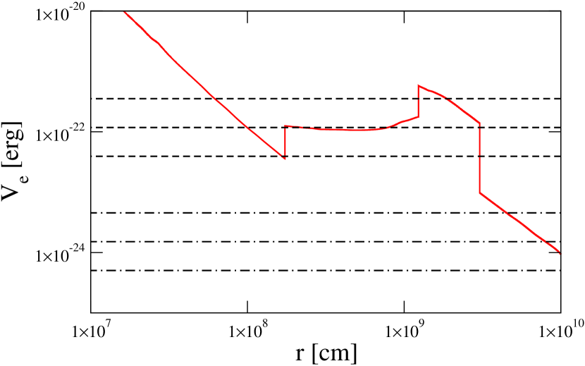
The profile we use for $\langle n_{e}(r)\rangle$ is the $t=3\;{\rm s}$ postbounce snapshot from the $10.8\;M_{\odot}$ simulation by Fischer et al. Fischer:2009 . The MSW potential for this profile is shown in figure (1) and was chosen so that neutrinos with the MSW resonance of the three energies we shall use throughout this paper, $5\;{\rm MeV}$, $15\;{\rm MeV}$ and $45\;{\rm MeV}$, intersect the profile in the region where we shall place the turbulence. As we shall discover, these energies are representative in the sense that each will be affected by the turbulence to differing degrees because the region where we place the turbulence will have a different relation to the MSW densities of these three neutrino energies. Since we are considering different neutrino energies it is not necessary for us to consider snapshots at other epochs from this simulation because, to first order, the profile epoch and the neutrino energy are degenerate: what occurs to lower energy neutrinos at early times will occur for higher energies at later times. For this profile we may regard the $45\;{\rm MeV}$ neutrinos as representing what we expect at the epoch when turbulence is just beginning to affect the neutrinos of a given energy, the $15\;{\rm MeV}$ as representing the effect when the H resonant channel is strongly affected, and the $5\;{\rm MeV}$ neutrinos as representing what we expect when the turbulence begins to affect both H and L resonant channels. Fixing the neutrino energy and changing the snapshot time would be an alternative way to explore this dependence between the turbulence effects and MSW densities. Also, the actual shape of the underlying one-dimensional profile is not very important to the turbulence effects so changing the simulation will not lead to qualitatively different results - the reader is referred to Lund & Kneller 2013PhRvD..88b3008L where turbulence was put into this same $M=10.8\;M_{\odot}$ simulation from Fischer et al. at multiple post-bounce epochs and compared with results for turbulence inserted into two other two simulations, a $M=8.8\;M_{\odot}$ and a $M=18\;M_{\odot}$, by the same authors.

Figure 2: In the left figure we show the evolution of the neutrino transition probability $P_{12}$ (dashed dot), $P_{13}$ (dashed) and $P_{23}$ (solid) with energies of $5\;{\rm MeV}$ (top panel) $15\;{\rm MeV}$ (middle panel) and $45\;{\rm MeV}$ (bottom panel) through the profile shown in figure (1). The right figure we show the evolution of the antineutrino transition probabilities $\bar{P}_{12}$ (dashed dot), $\bar{P}_{13}$ (dashed) and $\bar{P}_{23}$ (solid) with energies of $5\;{\rm MeV}$ (top panel) $15\;{\rm MeV}$ (middle panel) and $45\;{\rm MeV}$ (bottom panel) through the same profile.)

Returning to figure (1), the reader will observe there are three discontinuities within the profile: the reverse shock at $r_{r}=1,734\;{\rm km}$, the contact discontinuity at $r_{c}=12,348\;{\rm km}$ and the forward shock at $r_{f}=30,323\;{\rm km}$. These features were steepened by hand from the original simulation data: see Lund & Kneller 2013PhRvD..88b3008L for a discussion of why this steepening was necessary.

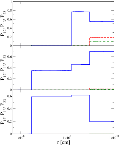
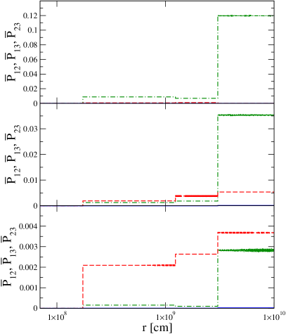
The evolution of neutrinos and antineutrinos with energies $5\;{\rm MeV}$, $15\;{\rm MeV}$ and $45\;{\rm MeV}$ and the given set of mixing parameters through the base profile are shown in figure (2). For the neutrinos the mixing between $\nu_{2}$ and $\nu_{3}$ dominates and note that the sudden discontinuities in the transition probability $P_{23}$ occur at the discontinuities in the profile and not at the MSW resonances (unless the two coincide). For $5\;{\rm MeV}$ neutrinos there is a noticeable change in both $P_{12}$ and $P_{13}$ at the forward shock; for the $15\;{\rm MeV}$ the change in the same probabilities at the same location is much smaller and by $45\;{\rm MeV}$ the change in $P_{12}$ and $P_{13}$ are minuscule. In the antineutrinos we again see a noticeable jump in $\bar{P}_{12}$ at the forward shock of similar size to the change of $P_{12}$ for neutrinos of the same energy while the jump in $\bar{P}_{12}$ at higher energies is much smaller; any jump in $\bar{P}_{23}$ is very small at all antineutrino energies (the mixing in this channel is suppressed if the mixing in $\nu_{2}-\nu_{3}$ is strong); and similarly the jumps in $\bar{P}_{13}$ are small for all energies. For future reference, the values of the transition probabilities $\{P_{12},P_{13},P_{23}\}$ and $\{\bar{P}_{12},\bar{P}_{13},\bar{P}_{23}\}$ through this profile for $5\;{\rm MeV}$ neutrinos are $\{0.0918,0.189,0.548\}$ and $\{0.120,7.09\times 10^{-5},3.12\times 10^{-5}\}$ respectively, for $15\;{\rm MeV}$ neutrinos they are $\{7.13\times 10^{-3},0.0308,0.696\}$ and $\{0.0353,5.36\times 10^{-3},1.35\times 10^{-4}\}$, for $45\;{\rm MeV}$ neutrinos they are $\{2.22\times 10^{-3},6.73\times 10^{-4},0.194\}$ and $\{2.81\times 10^{-3},3.68\times 10^{-3},1.85\times 10^{-5}\}$. The evolution of the neutrinos and antineutrinos through the underlying base profile will determine the extent to which turbulence is able to modify the emerging probabilities. In general we find that if $P_{ij}$ is close to the limits of zero or unity then the effect of turbulence tends to be smaller, everything else being equal. Thus we should expect big effects in $P_{23}$ even at small turbulence amplitudes while effects in $P_{12}$, $P_{13}$ and the antineutrinos will require somewhat larger density fluctuations.

It is in the region between the forward and reverse shocks that strong turbulence is seen in multi-dimensional simulations 2007A&A…467.1227A ; 2008PhRvD..77d5023K ; 2013arXiv1310.7488B so that is where we shall modify the profile to insert the turbulence. As in Lund & Kneller 2013PhRvD..88b3008L , we use two random field realizations: one for the zone between the forward shock and the contact discontinuity, and a second between the contact discontinuity and the reverse shock. Realizations are generated by multiplying $\langle n_{e}(r)\rangle$ by a factor $1+F(r)$ where $F(r)$ is a Gaussian random field with a power spectrum $E$. Quite generally we may write the random field $F(r)$ within the region $r_{<}$ to $r_{>}$ as a Fourier series of the form

$$\begin{split}F(r)&=C_{\star}\,\tanh\left(\frac{r-r_{<}}{\lambda_{\star}}\right)\,\tanh\left(\frac{r_{>}-r}{\lambda_{\star}}\right)\\ &\times\sum_{a=1}^{N_{q}}\,\sqrt{V_{a}}\left\{A_{a}\cos\left(q_{a}\,r\right)+B_{a}\sin\left(q_{a}\,r\right)\right\}.\end{split}$$ (2)

The purpose of the two $\tanh$ functions is to damp the fluctuations close to $r_{<}$ and $r_{>}$ and the parameter $\lambda_{\star}$ is the damping scale which we set to $\lambda_{\star}=100\;{\rm km}$. The parameter $C_{\star}$ is the root-mean-square amplitude of the field and we shall use the same value of $C_{\star}$ for the two realizations for simplicity. The set of co-efficients $\{A\}$ and $\{B\}$ are independent standard, zero-mean Gaussian random variates (which ensures the mean value of $F$ is zero), the wavenumbers for the Fourier modes are $q_{a}$ and the quantities $V_{a}$ are ‘volume’ co-efficients. The method for generating a realization of the turbulence is the same ‘variant C’ of the Randomization Method described in Kramer, Kurbanmuradov, & Sabelfeld 2007JCoPh.226..897K and used in Kneller & Mauney 2013PhRvD..88b5004K . The space of wavenumbers is divided into $N_{q}$ regions and from each region we select a random wavenumber $q$ using the normalized power-spectrum, $E(q)$, as a probability distribution. The volume parameters $V_{a}$ are the integrals of the power spectrum over each region. In order to produce random fields that affect the neutrinos we must cover a sufficiently large dynamic range of scales. Given the size of the turbulence regions shown in figure (1) and the neutrino oscillation lengthscale of $\sim 10\;{\rm km}$ at these densities, the dynamic range is found to be of order 40-50 decibels which requires at a minimum that $N_{q}$ also be in the range 40-50 2013PhRvD..88d5020K .

The power spectrum of the random field is taken to be an inverse power law of the form

$$E(q)=\frac{(\alpha-1)}{2\,q_{\star}}\left(\frac{q_{\star}}{|q|}\right)^{\alpha}\,\Theta(|q|-q_{\star}).$$ (3)

Here $\alpha$ is the spectral index and $q_{\star}$ is the long wavelength, small wavenumber, cutoff. The parameter $q_{\star}$ is sometimes called the ‘driving scale’ since it is the longest, non-zero turbulence wavelength. In our case this wavelength is twice the size of the turbulence domains, that is, $1/q_{\star}=2\,(r_{>}-r_{<})$. The assumption that the power spectrum $E$ has no spatial dependence is the simplest choice we can make but it’s an assumption that should be examined further. Though there is evidence that the power spectrum of the angular kinetic energy during the accretion phase does show radial dependence 2011ApJ…742…74M ; BlondinReyes , that does not automatically mean we should find radial dependence in the turbulence power spectrum during the cooling phase when the turbulence is far out in the stellar mantle. Similarly we know of no evidence that the turbulence power spectrum in a three dimensional simulation of a supernova at the appropriate epoch over the range of lengthscales we require is anything other than a single inverse power law: the broken power law found by Borriello et al 2013arXiv1310.7488B is relic of the two dimensional nature of the simulation they analysed.

With the Hamiltonian including turbulence constructed our plan is to generate multiple realizations of the turbulence and then solve equation (1) for the evolution matrix for each realization. This approach will allow us to construct ensembles of results which we can then characterize with frequency distributions or with distribution moments.

Figure 3: The evolution of $P_{23}$ as a function of distance $r$ for a $15\;{\rm MeV}$ neutrino. The dashed line is the evolution through the underlying profile and the solid line is the evolution with a single realization of turbulence with spectral index $\alpha=5/3$. In the top panel $C_{\star}=10\%$, in the middle $C_{\star}=1\%$ and in the bottom $C_{\star}=0.1\%$

III The two effects of turbulence

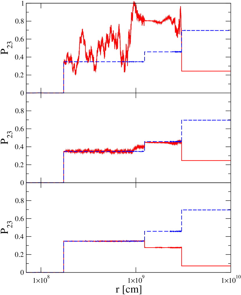
Before presenting the results from our numerical calculations, we first take time to demonstrate the two effects of turbulence. As we previously stated, the first effect is the modification of the neutrino transition probability evolution in the region of the turbulence due to direct stimulation between the states, and the second is the modification of the transition probabilities of the neutrino as it emerges from a turbulent region if the transition probabilities are subject to phase effects. The two effects are neatly shown in figure (3) where we see the evolution of the transition probability $P_{23}$ as a function of distance through the profile shown in figure (1) for a $E=15\;{\rm MeV}$ neutrino. In the top panel where $C_{\star}=0.1$ we see the first case: the evolution of the transition probability with turbulence differs from the evolution without turbulence as soon as the neutrino enters the turbulence region. In the middle panel where $C_{\star}=10^{-2}$ we see a small differences between the evolution with and without turbulence as soon as the neutrino enters the turbulence but the jumps at the discontinuities are significantly larger. In the bottom panel where $C_{\star}=10^{-3}$ there is no apparent difference between the evolution with and without turbulence until the contact discontinuity. Beyond that point the two curves are different but exhibit no relative change until the neutrino passes through the forward shock where another large change occurs. In these bottom two panels the change in the evolution is mainly due to a change in the phase effects; phase effects do occur in the top panel but are subordinate. But note well that that even though the turbulence amplitude differs by two orders of magnitude between the three calculations, the value of $P_{23}$ that emerges is very similar in each case.

In addition to the visual distinction between the two effects, it is possible to understand these two effects in more analytic terms. These analytic descriptions will prove useful because they allow us to construct expectations for, and thus interpret, the results from ensembles of realizations of the turbulence which we shall present in section §IV.

III.1 Phase effect distortion

Let us first concentrate on the distortion of the phase effect. We shall use a two-flavor model and a profile with two discontinuities which will be found to both adequately describe our results and to understand the effect. In the matter basis in which we work, figure (3) indicates that when the turbulence amplitude is small the neutrino passes through a set of discontinuities at the entrance and exit of the turbulent regions but evolves adiabaticaly in the turbulence region between the discontinuities. We can construct an evolution matrix which describes this evolution and from it derive the transition probability. First, the matter basis evolution matrix describing the evolution across a discontinuity located at $r$ is $S(r_{+},r_{-})=\tilde{U}^{\dagger}(r_{+})\tilde{U}^{\dagger}(r_{-})$ where $\tilde{U}$ is the matter mixing matrix ,$r_{-}$ is a point immediately before the discontinuity and $r_{+}$ a point immediately after. Adiabatic evolution of the neutrino between discontinuities means the evolution matrix must be of the form

$$S(r_{b},r_{a})=\left(\begin{array}[]{cc}\exp(-\imath\phi_{1})&0\\ 0&\exp(-\imath\phi_{2})\end{array}\right)$$ (4)

where

$$\phi_{j}=\int_{r_{a}}^{r_{b}}\,\tilde{k}_{j}(r)\,dr$$ (5)

and $\tilde{k}_{j}(r)$ is the instantaneous eigenvalue for matter state $j$. Thus the evolution matrix describing the neutrino evolution through a profile with two discontinuities, located at $r_{a}$ and $r_{b}$ is

$$S \sim \tilde{U}^{\dagger}(r_{b+})\tilde{U}^{\dagger}(r_{b-})\left(\begin{array}[]{cc}\exp(-\imath\phi_{1})&0\\ 0&\exp(-\imath\phi_{2})\end{array}\right)$$ (9)

$$\times\tilde{U}^{\dagger}(r_{a+})\tilde{U}^{\dagger}(r_{a-})$$

where we have omitted the evolution up to $r_{a-}$ and beyond $r_{b+}$ assuming it to be adiabatic. If we denote by $P_{a}$ and $P_{b}$ the crossing probabilities through the discontinuities separately, we find the crossing probability for the neutrino after passing through the entire profile is

$$P = P_{a}\,(1-P_{b})+(1-P_{a})\,P_{b}$$ (10)

$$+2\sqrt{P_{a}\,P_{b}\,(1-P_{a})(1-P_{b})}\,\cos(\Phi).$$

where $\Phi=\phi_{1}-\phi_{2}+constant$. Note well that $P_{a}$ and $P_{b}$ are constants and not changed when we insert turbulence into the profile and that $P_{a}\propto|\tilde{U}_{e1}^{\star}(r_{a+})\tilde{U}_{e2}(r_{a-})|^{2}$ and $P_{b}\propto|\tilde{U}_{e1}^{\star}(r_{b+})\tilde{U}_{e2}(r_{b-})|^{2}$. This dependence of $P$ upon the matter mixing matrix elements indicates the crossing probability $P$ is most sensitive to the turbulence via the distorted phase effect when the the MSW resonance density is similar to one of the densities on either side of the discontinuity.

The place where the turbulence enters equation (10) is via the phase difference $\Phi$. Every realization of the turbulence will give a different value for the phase difference and if we generate many realizations then we generate a distribution of phase differences. Thus we can model the effect of the turbulence by treating the phase difference $\Phi$ as a random variate drawn from a distribution $f(\Phi)$. The model we adopt for the distribution of $\Phi$ is the von Mises distribution which is of the form

$$f(\Phi)=\frac{\exp(\kappa\cos(\Phi-\Phi_{0}))}{2\pi I_{0}(\kappa)}$$ (11)

where $\Phi_{0}$ is the mean value of $\Phi$ and $\kappa$ is the concentration. If we define $P_{\star}=P_{a}\,(1-P_{b})+(1-P_{a})\,P_{b}$ and $\Delta=2\sqrt{P_{a}\,P_{b}\,(1-P_{a})(1-P_{b})}$ and note that $|dP/d\Phi|=\Delta\sin\Phi$ then we derive the distribution for $P$ must be

$$f(P) = \frac{1}{2\pi I_{0}(\kappa)\sqrt{\Delta^{2}-(P-P_{\star})^{2}}}$$ (12)

$$\times\exp\left(\kappa\cos\left[\cos^{-1}\left(\frac{P-P_{\star}}{\Delta}\right)-\Phi_{0}\right]\right)$$

on the interval $P_{\star}-\Delta\leq P\leq P_{\star}+\Delta$. In the limit where $\kappa\rightarrow 0$, the distribution of $\Phi$ is rectangular and the probability distribution for $P$ becomes the arcsine distribution i.e.

$$f(P)=\frac{1}{2\pi\sqrt{\Delta^{2}-(P-P_{\star})^{2}}}$$ (13)

which has a mean of $P_{\star}$ and variance of $V(P)=\Delta^{2}/2$. Note that in this limit there is no explicit dependence of $f(P)$ upon the spectral index $\alpha$ nor $C_{\star}$ because $P_{\star}$ and $\Delta$ are independent of the turbulence.

In the other limit where the concentration is large we can expand the phase $\Phi$ around $\Phi_{0}$ so that to lowest order (assuming $\sin\Phi_{0}\neq 0$)

$$P-P_{0}=-\Delta\sin(\Phi_{0})\,(\Phi-\Phi_{0})$$ (14)

where $P_{0}=P_{\star}+\Delta\cos\Phi_{0}$. This equation shows $P$ and $\Phi$ are linearly related in this limit and so the standard deviation of $P$ is proportional to the the standard deviation of $\Phi$: $\sigma_{P}\propto\sigma_{\Phi}$. The phase difference $\Phi$ between two discontinuities is given by

$$\Phi\propto\int_{r_{a}}^{r_{b}}\,\left(\tilde{k}_{i}(r)-\tilde{k}_{j}(r)\right)\,dr$$ (15)

and for neutrinos far from a MSW resonance - such as the $45\;{\rm MeV}$ neutrinos in the $\nu_{2}-\nu_{3}$ mixing channel - the difference between $\tilde{k}_{2}$ and $\tilde{k}_{3}$ is approximately the MSW potential $\langle V\rangle(1+F)$ in the region where we place the turbulence. This means we can write an expression for the variance of $\Phi$ which is

$$\langle(\Phi-\Phi_{0})^{2}\rangle\approx\langle\left(\int_{r_{a}}^{r_{b}}\,\langle V\rangle(r)F(r)\,dr\right)^{2}\rangle$$ (16)

The integral is dominated by the longer wavelengths, lowest wavenumbers of the random field $F$ - the integral over the turbulence modes with wavelengths smaller than the scale height of the potential will be very small. If we ignore all the Fourier modes except the lowest then we predict $\langle(\Phi-\Phi_{0})^{2}\rangle\propto\langle A_{1}^{2}\rangle$ and, since $q_{1}\approx q_{\star}$, we have $\langle A_{1}^{2}\rangle\propto\alpha-1$. Putting this together with the linear relationship between $P$ and $\Phi$ we conclude

$$\sigma_{P}\propto\sqrt{\alpha-1.}$$ (17)

This result indicates harder turbulence power spectra have less effect upon the transition probability than softer spectra. This makes sense because for phase distortion the neutrinos are more sensitive to the longest wavelength of the turbulence and those amplitudes increase with $\alpha$.

Obviously the distorted phase effect of turbulence requires a phase effect be present in the transition probability in the absence of turbulence. Glancing at figure (2) we see only $P_{23}$ has a strong phase effect with two or more semi-adiabatic transitions at the three energies we are using, plus $P_{12}$ and $\bar{P}_{12}$ for the $5\;{\rm MeV}$ neutrinos: in all other mixing channels the jumps in $P_{ij}$ at the discontinuities are too small. Thus we expect to see the distorted phase effect of turbulence for all three energies we are using in the $\nu_{2}-\nu_{3}$ mixing channel, and maybe a small distorted phase effect in $\nu_{1}-\nu_{2}$ and $\bar{\nu}_{1}-\bar{\nu}_{2}$ at $5\;{\rm MeV}$.

III.2 Stimulated transitions

A detailed description of the direct stimulation of transitions between neutrino states by turbulence can be found in Kneller, McLaughlin & Patton Kneller:2012id and the two papers by Patton, Kneller & McLaughlin 2014PhRvD..89g3022P ; 2015PhRvD..91b5001P . In this description the effect of the turbulence can be understood as similar to the effect of a laser upon a polarized molecule. Comparison between numerical and analytical solutions reveals the description to be very powerful because it is able to predict the effect of turbulence on a case-by-case basis. For every pair of neutrino matter states $i$ and $j$ there is an associated splitting $\delta k_{ij}$ between two eigenvalues of the Hamiltonian. As equation (2) indicates, turbulence can be described with a Fourier series and one finds that transitions between the neutrino states will be occur if a set of integers $\{n\}$ can be found, one for each Fourier mode, such that $\delta k_{ij}+\sum_{a}n_{a}q_{a}\approx 0$. When the condition is exact, known as a parametric resonance Ermilova ; Akhmedov ; 1989PhLB..226..341K ; 1996PhRvD..54.3941B ; 2009PhLB..675…69K , the amplitude of the transition between states $i$ and $j$ is $100\%$ no matter the amplitudes of each Fourier mode. Where the amplitudes of the modes enter is through the distance $\lambda$ - called the transition wavelength - over which a neutrino makes the transition from state $i$ to state $j$ or vice versa. This distance is inversely proportional to the coupling between the two states i.e. $\breve{U}_{ei}\,\breve{U}_{ej}^{\star}$, where $\breve{U}_{ei}$ are elements of the unperturbed matter mixing matrix, and also inversely proportional to a product of Bessel functions $J_{n_{a}}(z_{a})$ where $z_{a}\propto C_{a}/q_{a}$ and the integer $n_{a}$ is the same integer previously identified. $C_{a}$ is the amplitude of the Fourier mode $a$. In order for a stimulated transition to occur one must compare $\lambda$ with the density scale height $r_{\rho}$ of the underlying profile defined to be $r_{\rho}=\rho/(d\rho/dr)$. Only if $\lambda<r_{\rho}$ is a transition expected, if $\lambda>r_{\rho}$ then none will occur. Finally, the only difference when one considers antineutrinos is that the splitting $\delta k_{ij}$ and coupling $\breve{\bar{U}}_{ei}\,\breve{\bar{U}}_{ej}^{\star}$ are computed using a Hamiltonian where the MSW potential switches sign.

At small $C_{\star}$ one typically finds the integers are $n_{a}=0$ for all $a$ except for the mode whose wavenumber is closest to the eigenvalue splitting $\delta k_{ij}$ 2015PhRvD..91b5001P . In this limit the smallness of $C_{a}$ indicates $z_{a}$ for that mode will also be small so we may use $J_{1}\sim z$ for small $z$. Putting this all together we find the transition wavelength in the small amplitude limit goes as

$$1/\lambda\propto C_{a}\breve{U}_{ei}\,\breve{U}_{ej}^{\star}/q_{a}.$$ (18)

The transition wavelength $\lambda$ is inversely proportional to that resonant mode’s amplitude $C_{a}$ - which depends upon $\alpha$ and $C_{\star}$ - and the product of mixing matrix elements $\breve{U}_{ei}\,\breve{U}_{ej}^{\star}$ in the region of the turbulence. In order to make $\lambda$ small and see stimulated transition we must either increase $\breve{U}_{ei}\,\breve{U}_{ej}^{\star}$ and/or $C_{a}$. Increasing $\breve{U}_{ei}\,\breve{U}_{ej}^{\star}$ means the turbulence must be in the vicinity of the MSW density because the product takes on its maximal value at that location. This is the same requirement as in the distorted phase effect. Since the expectation value of $C_{a}$ goes as $\langle C_{a}\rangle^{2}=C_{\star}^{2}(q_{\star}/q_{a})^{\alpha}$ we see increasing $C_{a}$ can be achieved by either increasing $C_{\star}$ or decreasing $\alpha$.

The evolution of the underlying profile means the splitting between the neutrino eigenvalues $\delta k_{ij}$ and the coupling $\breve{U}_{ei}\,\breve{U}_{ej}^{\star}$ between the matter states both evolve with $\langle V\rangle$. This means neutrinos experience a parametric resonance only at a point and at present it is only possible to predict where and with what approximate strength the transitions occur. Phenomenologically one finds the distributions of the transition probabilities are exponentially distributed with greater widths as $C_{\star}$ and $\breve{U}_{ei}\,\breve{U}_{ej}^{\star}$ increase 2010PhRvD..82l3004K .

In the limit of large turbulence amplitudes and optimally placed turbulence, stimulated transitions occur essentially continuously in the turbulence region - the parametric resonance condition is fulfilled many times through the profile - and in virtually all realizations. When this occurs one finds the evolution matrix for the evolution between the discontinuities becomes essentially random rendering the evolution across the discontinuities unimportant. In this strong stimulated transition limit an ensemble of evolution matrices approaches that of an ensemble of $N$-flavor circular unitary matrices 1962JMP…..3..140D where the distribution of every element of the matrices is identical. This limit is known as depolarization and from the expectation for the structure of the ensemble of evolution matrices we can derive the distributions of the transition probabilities. First, we note that the $N$ real components, $x_{ij}$, plus the $N$ imaginary components, $y_{ij}$, of the elements of a row or column in every evolution matrix form a 2$N$ Euclidean space. The requirement of unitarity of the evolution matrix is equivalent to the definition that a vector made from these real and imaginary components lies upon the surface of a unit sphere in this space. Since these 2$N$ quantities are identically distributed, the probability $f$ of a particular set of the elements from a row or column must be uniform over the surface of the sphere. For example, if we chose to look at a column $j$ then the probability that we are located at $\{x_{1j},y_{1j},x_{2j},y_{2j},\ldots\}$, must be proportional to the area element $dA$ allowing us to write

$$f(x_{1j},y_{1j},x_{2j},y_{2j},\ldots)d^{N}xd^{N}y\propto dA$$

$$\;=\delta\left(1-\sum_{i=1}^{N}x_{ij}^{2}-\sum_{i=1}^{N}y_{ij}^{2}\right)\,\prod_{i=1}^{N}dx_{ij}\,\prod_{i=1}^{N}dy_{ij}.\;\;\;\;$$ (19)

If we now change variables so that each of the $N$ independent pairs $x_{ij},y_{ij}$ are expressed as

$$x_{1j}=\sqrt{P_{1j}}\,\cos\theta_{1j}, y_{1j}=\sqrt{P_{1j}}\,\sin\theta_{1j},$$ (20)

$$x_{2j}=\sqrt{P_{2j}}\,\cos\theta_{2j}, y_{2j}=\sqrt{P_{2j}}\,\sin\theta_{2j},$$ (21)

then the $P_{ij}$’s are found to be distributed as

$$f(P_{1j},\ldots P_{Nj})d^{N}P\propto\delta\left(1-\sum_{i=1}^{N}P_{ij}\right)\,\prod_{i=1}^{N}dP_{ij}.$$ (22)

The set of transition probabilities $\{P_{1j},\ldots P_{Nj}\}$ are uniformly distributed on the surface of a standard $N-1$ simplex. Equation (22) can be integrated over $N-1$ of the $P_{ij}$’s and normalized so that we derive the final result that element $P_{ij}$ must be distributed according to

$$f(P_{ij})=(N-1)\,(1-P_{ij})^{N-2}.$$ (23)

The shape of the distribution is controlled by the number of flavors $N$ that are involved and nothing else. With the distribution for $P_{ij}$ found it is a simple task to determine that the mean and variance are

$$\langle P_{ij}\rangle = \frac{1}{N},$$ (24)

$$V(P_{ij}) = =\sigma_{ij}^{2}=\frac{N-1}{N^{2}\,(N+1)}$$ (25)

For the specific case of $N=2$ the distribution is uniform with mean $1/2$ and variance $1/12$: for $N=3$ the distribution is triangular with mean $1/3$ and variance $1/18$. Note that the depolarized limits do not explicitly depend upon any property of the turbulence, they are functions only of the appropriate number of flavors involved. It is via $N$ that the turbulence amplitude and spectral index will enter because the appropriate value of $N$ will change as $C_{\star}$ and $\alpha$ are varied.

Since there are three flavors of neutrino it would seem we should use the $N=3$ case but in practice whether 3-flavor depolarization is actually reached depends upon the placement of the turbulence in the profile in relation to the H and L resonance densities for a given energy. If not located in the appropriate place in the profile for a given neutrino energy, two flavor depolarization may be more appropriate. As we stated, the distance over which a neutrino makes the transition from matter state $j$ to matter state $i$ is proportional to the product of instantaneous mixing matrix elements $\breve{U}_{ei}\breve{U}_{ej}^{\star}$. This product has its maximal value at the resonance between states $i$ and $j$. Figure (1) shows that the H resonance density for the $E=45\;{\rm MeV}$ neutrinos is below the densities where we place the turbulence by a factor $\gtrsim 3$, the L resonance density is lower by a factor $\gtrsim 300$. For $E=45\;{\rm MeV}$ neutrinos we should expect some difficultly stimulating transitions between matter states $\nu_{1}$ and $\nu_{2}$ but it should be somewhat easier for mixing between states $\nu_{2}$ and $\nu_{3}$. For the lower energy of $15\;{\rm MeV}$ the H resonance density is very similar to the density of the profile between the reverse shock and the contact discontinuity which would lead us to expect a strong stimulated transition effect in this channel for this energy. The L resonance for this same energy again lies below the density of the profile meaning the product of mixing matrix elements $\breve{U}_{e1}\breve{U}_{e2}^{\star}$ will be small again suppressing stimulated transitions between $\nu_{1}$ and $\nu_{2}$. Finally, the H resonance density for the $5\;{\rm MeV}$ neutrinos is similar to the density of the profile between the contact discontinuity and the reverse shock and the difference between the L resonance density and the profile density between the reverse shock and the contact discontinuity is only of order a factor of a few. Thus of the three energies we are considering, the $5\;{\rm MeV}$ neutrinos have the best prospect of exhibiting stimulated transitions between all three states and reaching 3 flavor depolarization, the $E=15\;{\rm MeV}$ and $E=45\;{\rm MeV}$ neutrinos should show evidence for stimulated transition only between two states.

Figure 4: The mean values of $P_{12}$ (top row), $P_{13}$ (middle row) and $P_{23}$ (bottom row) as a function of the power spectral index.The leftmost column is for $5\;{\rm MeV}$ neutrinos, the middle for $15\;{\rm MeV}$ and the rightmost is $45\;{\rm MeV}$. In all panels the curves correspond to $C_{\star}=0.5$ (filled circles), $C_{\star}=0.3$ (filled squares), $C_{\star}=0.1$ (filled diamonds), $C_{\star}=10^{-2}$ (filled triangles), $C_{\star}=10^{-3}$ (open circles), $C_{\star}=10^{-4}$ (open squares) and $C_{\star}=10^{-5}$ (open diamonds). For the sake of clarity, not all lines appear in each panel; where a line is missing it should be taken to be negligibly different from the smallest value of $C_{\star}$ shown in the panel.

Figure 5: The standard deviation of $P_{12}$ (top row), $P_{13}$ (middle row) and $P_{23}$ (bottom row) as a function of the power spectral index.The leftmost column is for $5\;{\rm MeV}$ neutrinos, the middle for $15\;{\rm MeV}$ and the rightmost is $45\;{\rm MeV}$. In all panels the curves correspond to $C_{\star}=0.5$ (filled circles), $C_{\star}=0.3$ (filled squares), $C_{\star}=0.1$ (filled diamonds), $C_{\star}=10^{-2}$ (filled triangles), $C_{\star}=10^{-3}$ (open circles), $C_{\star}=10^{-4}$ (open squares) and $C_{\star}=10^{-5}$ (open diamonds). Again, for the sake of clarity, not all lines appear in each panel; where a line is missing it should be taken to be negligibly different from the smallest value of $C_{\star}$ shown in the panel.

Figure 6: Frequency distribution of the transition probability $P_{23}$ for the case of a $45\;{\rm MeV}$ neutrino. The spectral index is set to $\alpha=5/3$ and, from top to bottom, the turbulence amplitude is $C_{\star}=10^{-3}$, $C_{\star}=10^{-4}$ and $C_{\star}=10^{-5}$.

The stimulated transitions work between the discontinuities in the profile while the evolution across the discontinuities themselves is still given by $\tilde{U}^{\dagger}(r_{+})\tilde{U}^{\dagger}(r_{-})$. Thus stimulated transitions and distorted phases do not work separately, they work in tandem. The essential difference between the two is for stimulated transitions one replaces the central evolution matrix in equation (9) which describes adiabatic evolution between the discontinuities with a matrix that may or may not have non-zero off diagonal elements depending upon whether there were any stimulated transitions in the turbulence region. Even if there are no stimulated transitions in the turbulence region, at a minimum the turbulence will distort the phase. For this reason we often find circumstances where the distributions for the transition probabilities in a given channel are not completely described by a distorted phase model nor solely described by stimulated transitions but rather exhibit contributions from both. These situations arise because stimulated transitions are often found to be ‘all-or-nothing’. Thus the frequency distributions of the transition probabilities in these circumstances are seen to be mixtures of two distinct, more fundamental, distributions - see for example figure (12) in Kneller & Volpe 2010PhRvD..82l3004K - which can cause difficulty with interpretation of results. Mixing between distributions will shift the means and variances of the total distribution from the expected values of the two, more fundamental, components. If the distribution Type A, with mean transition probability $\langle P\rangle_{A}$ and variance $\sigma^{2}_{A}$, contributes a fraction $f$ to the total distribution, and a different distribution, Type B, with mean transition probability $\langle P\rangle_{B}$ and variance $\sigma^{2}_{B}$ contributes $1-f$, then the mean transition probability of the total distribution is $\langle P\rangle=f\,\langle P\rangle_{A}+(1-f)\,\langle P\rangle_{B}$ and similarly the variance is also $\sigma^{2}=f\,\sigma^{2}_{A}+(1-f)\,\sigma^{2}_{B}$. One should expect the fraction $f$ to depend upon the neutrino energy and snapshot time as well as the turbulence amplitude $C_{\star}$ and the spectral index $\alpha$. Knowing $f$ is useful if one wants to, say, simulate supernova neutrino signals using Monte Carlo methods. The neutrinos we receive at a given instant from the next supernova in our galaxy will all have traveled through similar turbulence as they traversed the mantle of the star which has the consequence that the transition probabilities of the neutrinos of a given energy will be very strongly correlated - the size of the proto-neutron in not sufficient to wash this correlation out unless the turbulence is very anisotropic 2013PhRvD..88d5020K . This means that the neutrino signal will not have sampled the ensemble of realizations of the turbulence, we receive neutrinos which have been affected by essentially just one realization. The probability this realization gives transition probabilities distributed according to distribution Type A is the fraction $f$; the probability the transition probabilities are distributed according to distribution Type B is $1-f$.

IV Results

IV.1 Neutrinos

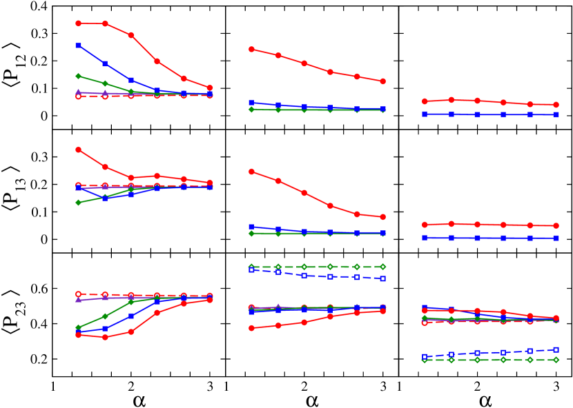
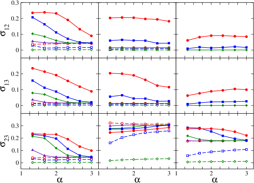
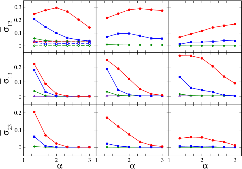
In figures (4) and (5) we show the mean values and standard deviation of the distributions of the neutrino transition probabilities $P_{12}$, $P_{13}$ and $P_{23}$ as a function of the spectral index and the turbulence amplitude for the three representative energies we are using. Even a cursory glance indicates there is a great deal of rich behavior as a function of the three parameters we have varied to generate the figures. Before diving into the results in depth to try and understand why we see the trends we do, let us summarize them:

• $E=45\;{\rm MeV}$. When $C_{\star}=50\%$, $\alpha\leq 7/3$ and $C_{\star}=30\%$, $\alpha\leq 5/3$, the $\nu_{2}$-$\nu_{3}$ mixing channel reaches $\langle P_{23}\rangle=0.5$ and $\sigma_{23}=0.28$. At these same large amplitudes but larger $\alpha$ we see the mean and standard deviation, $\langle P_{23}\rangle$ and $\sigma_{23}$ respectively, both fall with increasing $\alpha$. In the range $0.1\%\lesssim C_{\star}\lesssim 10\%$ it appears $\langle P_{23}\rangle$ is fixed at $\langle P_{23}\rangle=0.44$ independent of $\alpha$ and $C_{\star}$ and similarly the standard deviation $\sigma_{23}$ is also independent of $\alpha$ and $C_{\star}$ fixed at $\sigma_{23}\approx 0.18$. These same two values appear to be the asymptotic limits of $\langle P_{23}\rangle$ and $\sigma_{23}$ for $C_{\star}=50\%$ and $C_{\star}=30\%$ for large $\alpha$. At very small turbulence amplitudes, $C_{\star}\lesssim 0.01\%$, a dependence of $\langle P_{23}\rangle$ and $\sigma_{23}$ upon $C_{\star}$ and $\alpha$ re-emerges and it appears both $\langle P_{23}\rangle$ and the standard deviation $\sigma_{23}$ increase as the power spectrum becomes softer. In $\langle P_{12}\rangle$, $\langle P_{13}\rangle$, $\sigma_{12}$ and $\sigma_{13}$ we only see a difference from turbulence free results when $C_{\star}=50\%$ and $C_{\star}=30\%$ with little dependence upon $\alpha$.

• $E=15\;{\rm MeV}$. For this energy the mean value of $P_{23}$ is approximately $\langle P_{23}\rangle=0.5$ at $\alpha=3$ for all turbulence amplitudes above $C_{\star}=0.1\%$. Except for the case of $C_{\star}=0.5$, there is no apparent running of $\langle P_{23}\rangle$ with $\alpha$ or $C_{\star}$ in this range of amplitudes: in $\sigma_{23}$ the trend appears to be a small increase in $\sigma_{23}$ with $\alpha$ from $\sigma_{23}=0.28$ at $\alpha=4/3$ to $\sigma_{23}=0.3$ at $\alpha=3$ and we observe that at fixed $\alpha$, as $C_{\star}$ decreases the standard deviation increases. For $C_{\star}=0.5$ the increase of $\langle P_{23}\rangle$ and $\sigma_{23}$ with increasing $\alpha$ is more obvious and we note that $\langle P_{12}\rangle$, $\langle P_{13}\rangle$, $\sigma_{12}$ and $\sigma_{13}$ are noticeably different at $C_{\star}=0.5$ from even the case of $C_{\star}=0.3$. For $C_{\star}\lesssim 0.1\%$ the evolution of the standard deviation $\sigma_{23}$ with $C_{\star}$ reverses and now $\sigma_{23}$ decreases with $C_{\star}$. However, as with the $E=45\;{\rm MeV}$ neutrinos, the trend appears to be at very small turbulence amplitudes there is an increase of $\sigma_{23}$ and larger difference between the turbulence -free result of $\langle P_{23}\rangle$ with increasing $\alpha$.

• $E=5\;{\rm MeV}$. For this energy we observe much larger turbulent effects in the $\nu_{1}$-$\nu_{2}$ and $\nu_{1}$-$\nu_{3}$ mixing channels than for the other two energies considered particularly for small $\alpha$. When $C_{\star}=50\%$ and $\alpha\leq 5/3$ the mean values of $P_{12}$, $P_{13}$ and $P_{23}$ all plateau at $\langle P_{ij}\rangle=0.33$ and the standard deviations $\sigma_{12}$, $\sigma_{13}$ and $\sigma_{23}$ all reach $\sigma_{ij}=0.23$ in the same range of amplitudes and spectral indices. For all amplitudes greater than $C_{\star}\gtrsim 1\%$ the trend of $\langle P_{12}\rangle$, $\langle P_{13}\rangle$ and $\langle P_{23}\rangle$ with $\alpha$ is towards a fixed value with simultaneous decreasing standard deviations $\sigma_{12}$, $\sigma_{13}$ and $\sigma_{23}$. At small amplitudes for the turbulence, $C_{\star}\lesssim 1\%$, all three transition probabilities of the $5\;{\rm MeV}$ neutrinos approach the previously reported values through the underlying profile. The convergence is more rapid for softer power spectra: e.g.  at $C_{\star}=10\%$ the mean of $P_{12}$ and $P_{23}$ are measurably different from the turbulence free values at $\alpha=5/3$ but not so at $\alpha=7/3$.

Let us now examine these results in more detail and try to find explanations of the trends we observe using the two different descriptions for the effects of turbulence from section §III.

IV.1.1 $E=45\;{\rm MeV}$

We first examine the $E=45\;{\rm MeV}$ neutrinos and focus upon $P_{23}$. At large amplitudes and hard spectral indices the $\nu_{2}$-$\nu_{3}$ mixing channel appears to reach the two-flavor depolarized limit since $\langle P_{23}\rangle=0.5$ and $\sigma_{23}=0.28$ when $C_{\star}=50\%$ and $\alpha\leq 7/3$ and $C_{\star}=30\%$ and $\alpha\leq 5/3$. The decrease of $\langle P_{23}\rangle$ and $\sigma_{23}$ for the same large amplitudes but larger $\alpha$ is again in line with what we expect from stimulated transitions. The reduced amplitude of the modes that have wavelengths of order the eigenvalue splittings mean the stimulated transitions are not as strong and the distribution of $P_{23}$ will no longer be uniform.

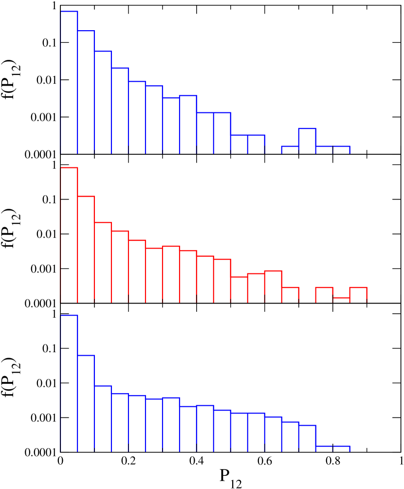
At smaller turbulence amplitudes our explanation for the results changes. In the range $0.1\%\lesssim C_{\star}\lesssim 10\%$ the mean value of $P_{23}$ and the standard deviation $\sigma_{23}$ are independent of $\alpha$ fixed at apparently arbitrary values. Only if we push further to even smaller turbulence amplitudes, $C_{\star}\lesssim 0.01\%$, do we see the dependence upon $C_{\star}$ and $\alpha$ re-emerge but when it re-emerges the trend that both $\langle P_{23}\rangle$ and the standard deviation $\sigma_{23}$ increase as the power spectrum becomes softer. This behavior of $\langle P_{23}\rangle$ and $\sigma_{23}$ for $C_{\star}\leq 10\%$ must be explained by using the distorted phase model so let us use this model to try and predict the actual values found in (4) and (5) for the $E=45\;{\rm MeV}$ neutrinos in this amplitude range. From analyzing the evolution without turbulence - figure (2) - we find the the transition probabilities for these neutrinos at the reverse and forward shocks give $P_{a}=0.57$ and at the second $P_{b}=0.93$. These can be combined to give $P_{\star}=0.44$ and $\Delta=0.25$. Since the transition probability in the absence of turbulence is $P_{23}=0.20$ we deduce $\Phi=163^{\circ}$. With this information in hand we predict the distribution of the transition probability $P_{23}$ when we insert the turbulence will lie in the range of $P_{\star}-\Delta=0.19$ to $P_{\star}+\Delta=0.69$. When the concentration $\kappa$ is small we expect an arcsine distribution for $P_{23}$ with a mean $\langle P_{23}\rangle=P_{\star}=0.44$ and standard deviation $\Delta/\sqrt{2}=0.18$. These predictions match the data well so we interpret our results as meaning that in the range $0.1\%\lesssim C_{\star}\lesssim 10\%$ the $45\;{\rm MeV}$ neutrinos are experiencing a strong distorted phase effect. At smaller turbulence amplitudes when the concentration $\kappa$ is larger the distribution will be like a half-Gaussian because the turbulence-free value of $P_{23}=0.20$ is close to the lower limit of the distribution.

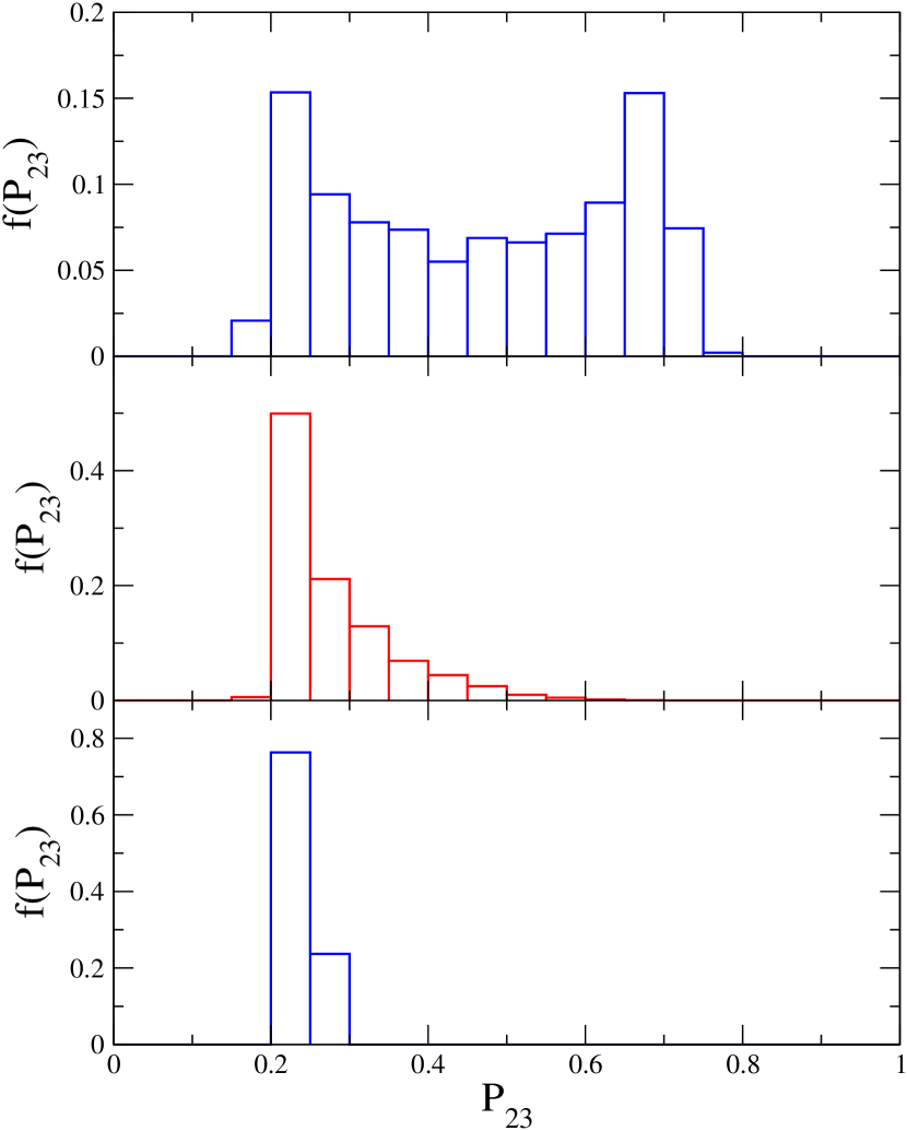
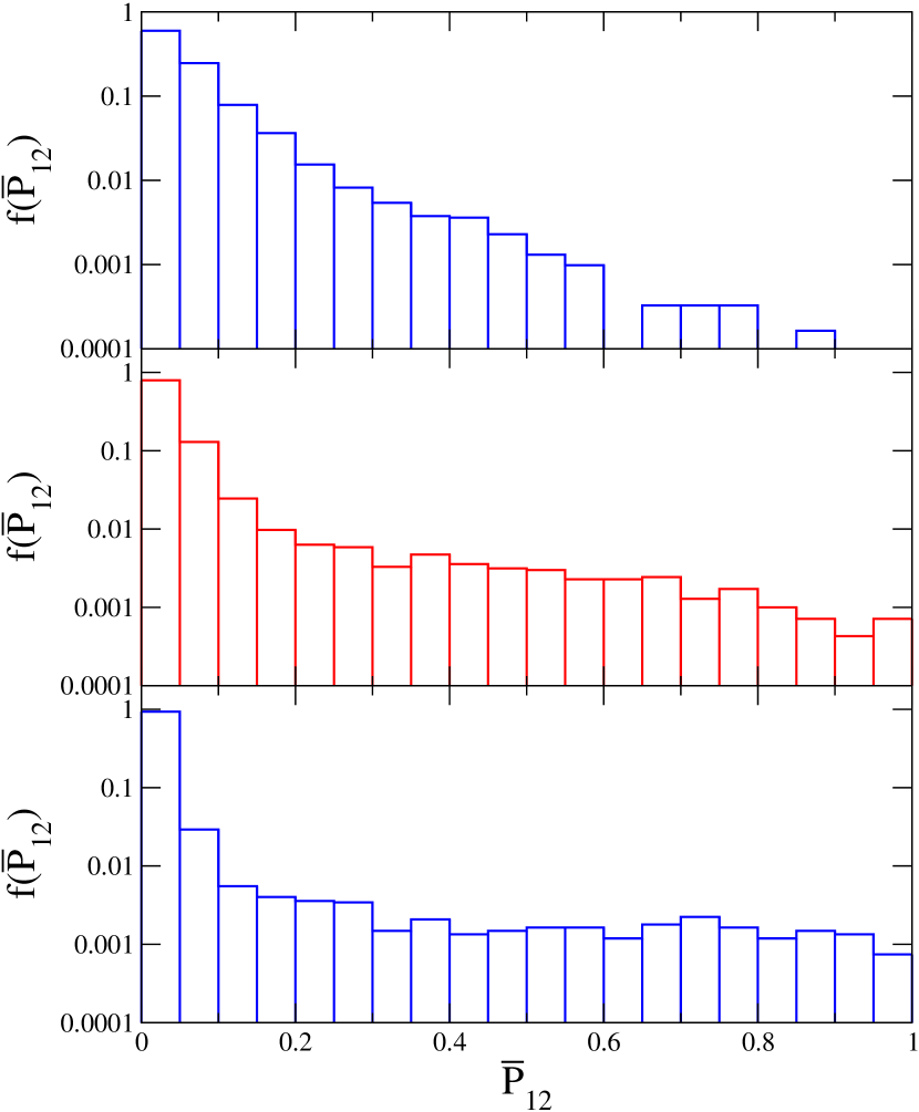
The frequency distribution of $P_{23}$ for $45\;{\rm MeV}$ neutrinos at $C_{\star}=10^{-3}$, $C_{\star}=10^{-4}$ and $C_{\star}=10^{-5}$ is shown in figure (6) and these expected shapes of the distributions is seen in the numerical results. At $C_{\star}=10^{-3}$ the distribution is symmetric around $P_{23}=0.44$ peaking at the extremes $P_{23}=0.19$ and $P_{23}=0.69$ as an arcsine distribution should. At $C_{\star}=10^{-4}$ and $C_{\star}=10^{-5}$ the symmetry is lost and the distribution looks more like an exponential or half-Gaussian. The running of $\langle P_{23}\rangle$ and $\sigma_{23}$ with $\alpha$ for the $E=45\;{\rm MeV}$ neutrinos and smaller turbulence amplitudes is also in line with our expectations from the distorted phase model because we see $\sigma_{23}$ increase with $\alpha$ e.g.  $C_{\star}=10^{-4}$.

Let us now consider the other mixing channels at this same energy. Compared to $P_{23}$, the mean of the transition probabilities $\langle P_{12}\rangle$ and $\langle P_{13}\rangle$ for the $E=45\;{\rm MeV}$ neutrinos appear quite unremarkable differing from the turbulence free limit only when $C_{\star}=0.5$ and then possessing only a soft dependence upon $\alpha$. The standard deviations $\sigma_{12}$ and $\sigma_{13}$ evolve similarly. At this energy the distorted phase effect of turbulence does not operate in these channels because the jumps in $P_{12}$ and $P_{13}$ across the discontinuities are small. The sensitivity to the turbulence is entirely through the stimulated transition mechanism. But as previously mentioned, the large separation between the turbulence densities and the L resonance MSW density at this energy means not every realization will cause a stimulated transition to occur in these channels so it is quite natural to expect the ensemble to be divided into two subsets. When we look we find this is exactly the case. The frequency distribution of the $P_{12}$ and $P_{13}$ transition probabilities are mixtures of a very narrow distribution which peaks at zero - the neutrinos unaffected by the turbulence - and an exponential distribution - the subset where stimulated transitions occurred.

Figure 7: The frequency distribution of $P_{23}$ for $15\;{\rm MeV}$ neutrinos at $\alpha=5/3$. In the top panel $C_{\star}=10\%$, in the middle panel $C_{\star}=1\%$, and in the bottom panel $C_{\star}=0.1\%$,

Figure 8: The frequency distribution of the neutrino transition probability $P_{12}$ when $E=15\;{\rm MeV}$ and $C_{\star}=0.3$. In the top panel $\alpha=4/3$, in the middle $\alpha=5/3$, and in the bottom panel $\alpha=2$.

Figure 9: The frequency distribution of the transition probabilities $P_{12}$, $P_{13}$ and $P_{23}$ for the case of a $5\;{\rm MeV}$ neutrino. The spectral index is $\alpha=4/3$ and the turbulence amplitude is $C_{\star}=0.5$.

Figure 10: The frequency distribution of $P_{12}$ for $E=5\;{\rm MeV}$ neutrinos at $C_{\star}=0.3$. In the top panel $\alpha=5/3$, in the middle $\alpha=7/3$, and in the bottom panel $\alpha=3$.

Figure 11: The mean values of $\bar{P}_{12}$ (top row), $\bar{P}_{13}$ (middle row) and $\bar{P}_{23}$ (bottom row) as a function of the power spectral index.The leftmost column is for $5\;{\rm MeV}$ neutrinos, the middle for $15\;{\rm MeV}$ and the rightmost is $45\;{\rm MeV}$. In all panels the curves correspond to $C_{\star}=0.5$ (filled circles), $C_{\star}=0.3$ (filled squares), $C_{\star}=0.1$ (filled diamonds), $C_{\star}=10^{-2}$ (filled triangles). For the sake of clarity, not all lines appear in each panel.

Figure 12: The standard deviation of $\bar{P}_{12}$ (top row), $\bar{P}_{13}$ (middle row) and $\bar{P}_{23}$ (bottom row) as a function of the power spectral index.The leftmost column is for $5\;{\rm MeV}$ neutrinos, the middle for $15\;{\rm MeV}$ and the rightmost is $45\;{\rm MeV}$. In all panels the curves correspond to $C_{\star}=0.5$ (filled circles), $C_{\star}=0.3$ (filled squares), $C_{\star}=0.1$ (filled diamonds), $C_{\star}=10^{-2}$ (filled triangles), $C_{\star}=10^{-3}$ (open circles), $C_{\star}=10^{-4}$ (open squares) and $C_{\star}=10^{-5}$ (open diamonds). Again, for the sake of clarity, not all lines appear in each panel.

Figure 13: The frequency distribution of the antineutrino transition probability $\bar{P}_{12}$ when $E=15\;{\rm MeV}$ and $C_{\star}=0.3$. In the top panel $\alpha=4/3$, in the middle $\alpha=5/3$, and in the bottom panel $\alpha=2$.

IV.1.2 $E=15\;{\rm MeV}$

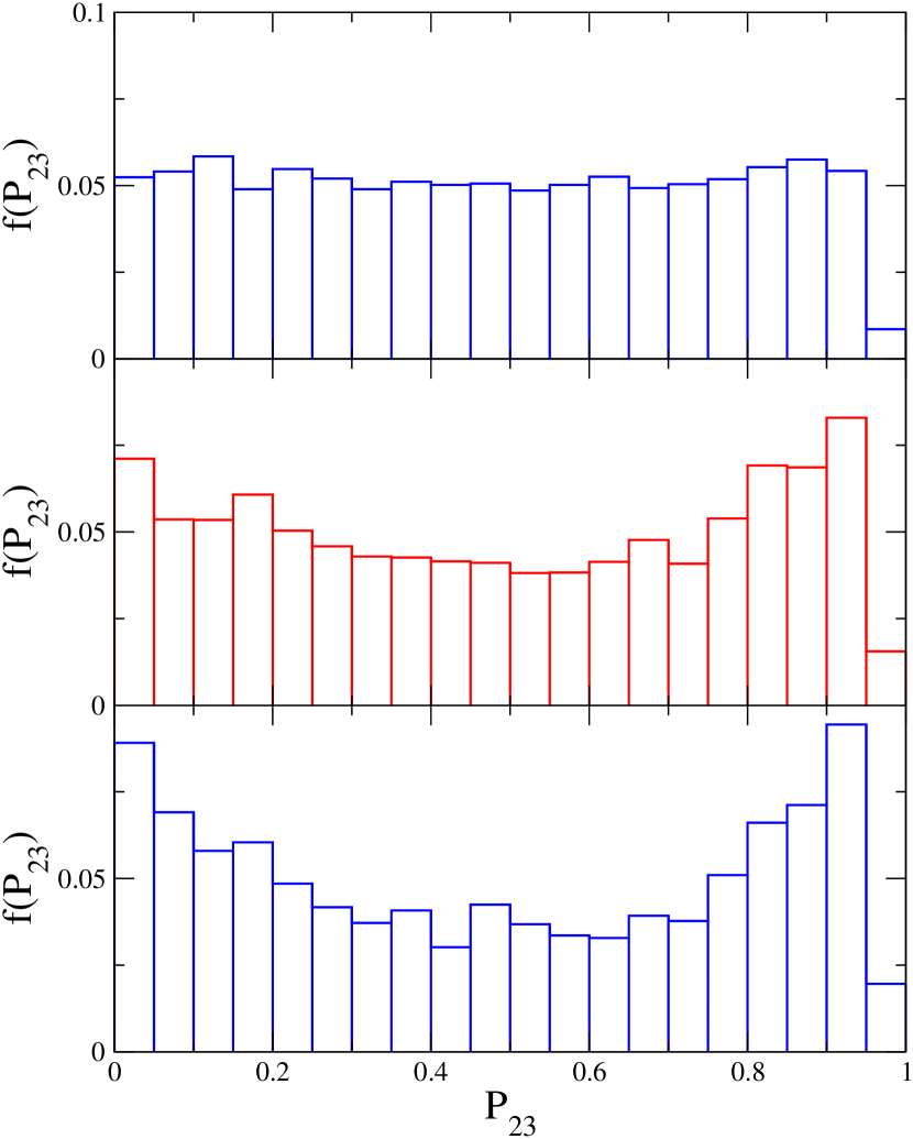
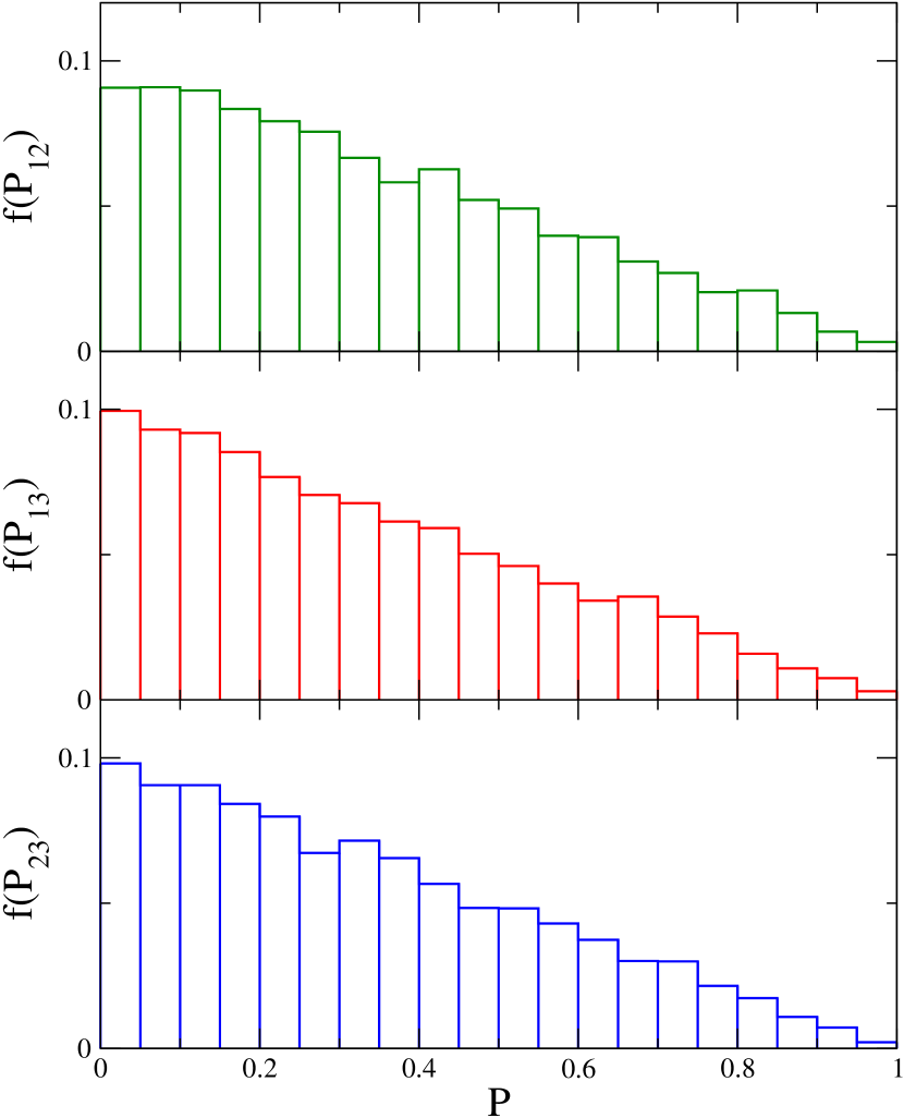
We now consider the energy $E=15\;{\rm MeV}$. For this energy the evolution of the distributions of $P_{23}$ is again explained by a transition from stimulated transitions at large $C_{\star}$/small $\alpha$ to the distorted phase effect at smaller $C_{\star}$/ larger $\alpha$. The frequency distributions of $P_{23}$ for $15\;{\rm MeV}$ neutrinos at fixed $\alpha=5/3$ as several amplitudes $C_{\star}$ are shown figure (7). In all three cases shown the mean value of $P_{23}$ is approximately the same, around $\langle P_{23}\rangle\approx 0.5$, but the distributions are clearly different depending upon $C_{\star}$: for the large amplitude $C_{\star}=0.1$ the distribution is almost uniform - the bin $0.95\leq P_{23}\leq 1$ appears low - whereas the distribution for $C_{\star}=0.001$ has a very peculiar shape with the extreme values of $P_{23}$ more common than the mean. These distributions reflect the two different mechanisms by which the turbulence affects the neutrinos - the top panel is what we would expect from stimulated transitions in the depolarized limit with two flavors whereas the distribution in the lower panels is the indirect, distorted phase effect since they are consistent with an arcsine distribution, similar to that seen in the top panel of figure (6), albeit on the interval of zero to unity.

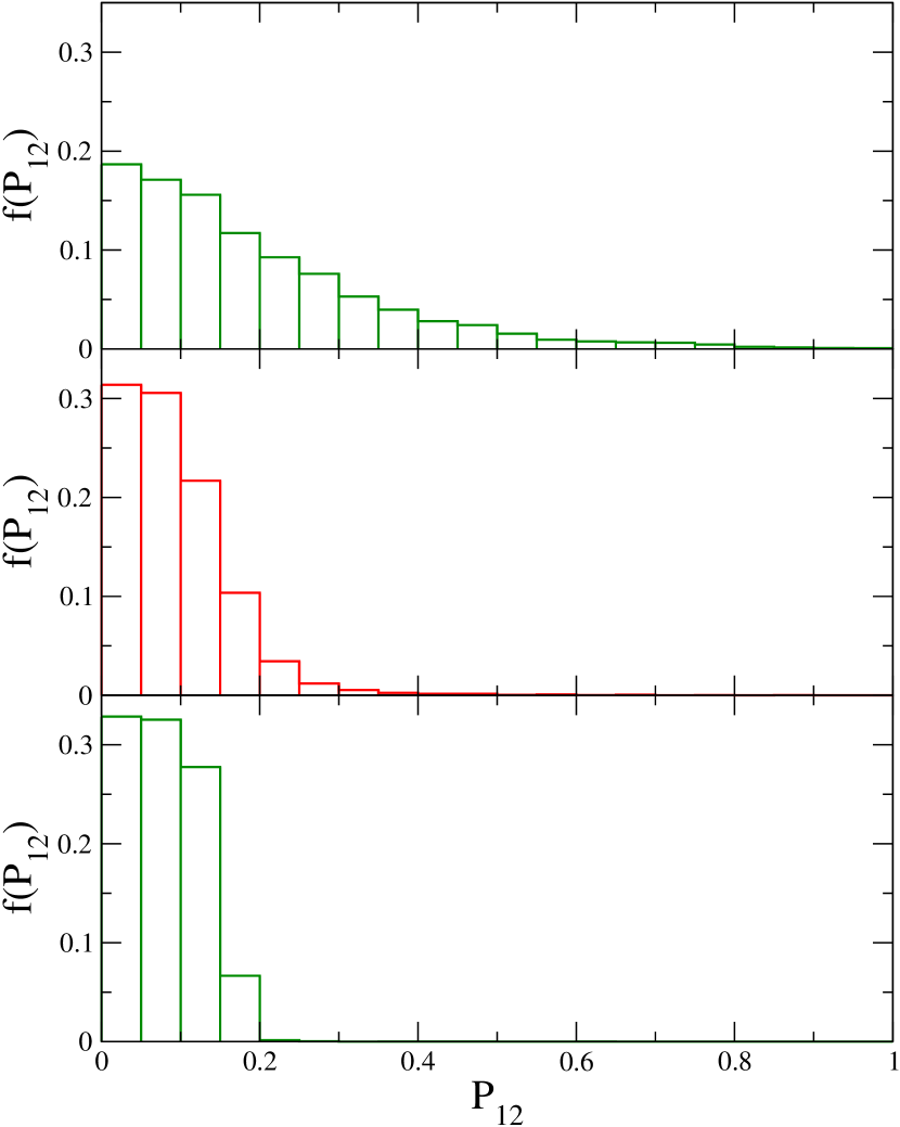
The mean values of $P_{12}$ and the standard deviations $\sigma_{12}$ shown in figures (4) and (5) do not match the expected values from the our model distributions and this is because, as with the $E=45\;{\rm MeV}$ neutrinos, we find the ensembles are mixtures of distributions. At $C_{\star}=0.5$ inspection indicates the mixing distributions in $\nu_{1}-\nu_{2}$ for this energy are a sharp distribution which peaks at zero - the neutrinos with no turbulence effects - and a three flavor depolarized distribution which are the neutrinos that experienced stimulated transitions. But when we consider a slightly smaller value of $C_{\star}=0.3$ we find the mixing distributions for $P_{12}$ are the same narrow distribution peaked at zero but the second distribution is now an exponential. The frequency distributions of $P_{12}$ at $C_{\star}=0.3$ and $E=15\;{\rm MeV}$ at three values of $\alpha$ are shown in figure (8) and in the figure we observe a flattening of the exponentially distributed component as $\alpha$ increases.

IV.1.3 $E=5\;{\rm MeV}$

Finally we switch to the $5\;{\rm MeV}$ neutrinos. Here neither the H resonance nor the L resonance are too far from the densities where we insert the turbulence so the product of instantaneous mixing matrix elements $\breve{U}_{ei}\,\breve{U}_{ej}^{\star}$ are not small in any mixing channel. This allows stimulated transitions to occur between all three states simultaneously. The simultaneous mixing in all three channels indicates we might find that at sufficiently large amplitudes and hard spectral indices we could reach three-flavor depolarization. When we look indeed this is found for $C_{\star}\gtrsim 50\%$ and $\alpha=4/3$ shown in figure (9) where we see the frequency distributions of the transition probabilities are triangular as predicted. Thus figures (4) and (5) reveal the three-flavor depolarized limit is reached for $P_{12}$ only for $C_{\star}=50\%$ and $\alpha\leq 5/3$ whereas the same limit appears somewhat easier to reach for $P_{23}$ because even $C_{\star}=10\%$ amplitude turbulence saturates at $\langle P_{23}\rangle=1/3$ and $\sigma_{23}=0.23$ for $\alpha=4/3$ or at $C_{\star}=50\%$ we are able to relax the spectral index to $\alpha=2$. This is not surprising given the location of the turbulence in the profile with respect to the $\nu_{2}-\nu_{3}$ mixing resonance density shown in figure (1). Note also the figures do not indicate there are combinations of $C_{\star}$ and $\alpha$ where we achieve two flavor depolarization instead of three because we do not see $\langle P_{23}\rangle\approx 0.5$ or $\sigma_{23}\approx 0.28$ as one would expect in that limit.

As we move to smaller turbulence amplitudes what we observe in figures (4) and (5) might seem at first to be contradictory. The mean transition probability in the ensembles is the same as the value in the turbulence free limit tempting one to conclude that turbulence has no effect, but the standard deviations do not support this conclusion because it is not until $C_{\star}\lesssim 0.001\%$ that the turbulence effect actually disappears. The contradictions can be resolved when one realizes what the figures are showing is that between $0.001\%\lesssim C_{\star}\lesssim 1\%$ the distributions of the transition probabilities are simply centered on the turbulence-free limits. As with the $E=45\;{\rm MeV}$ neutrinos, the acute sensitivity to $C_{\star}$ is due to the distorted phase effect with the twist that now both $P_{23}$ and $P_{12}$ (and $\bar{P}_{12}$) are affected.

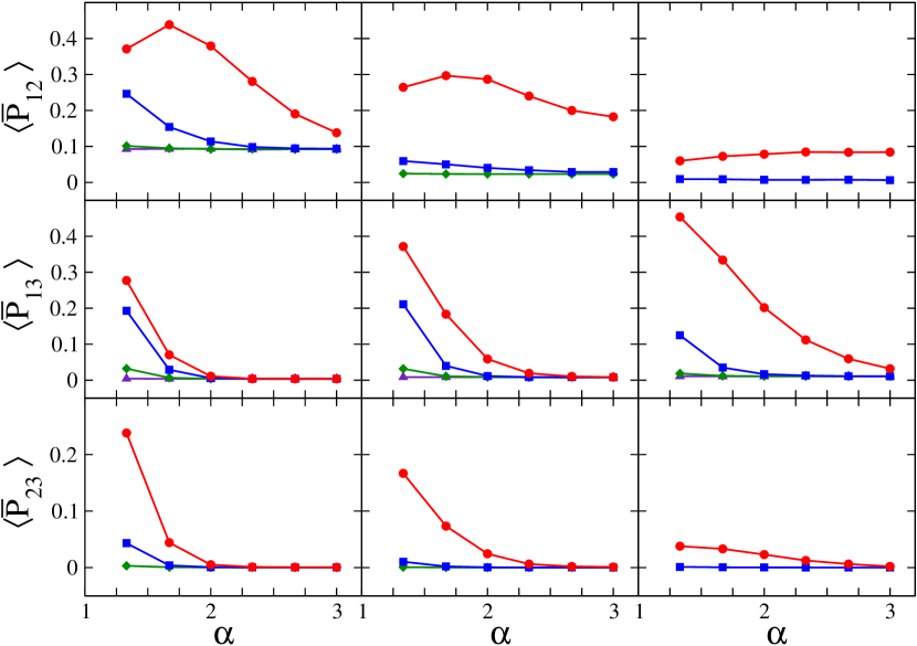
The distributions of $P_{12}$ and $P_{23}$ when $0.001\%\lesssim C_{\star}\lesssim 10\%$ are mixtures of an exponential and the distorted phase distributions and the evolution of $\langle P_{12}\rangle$ and $\langle P_{23}\rangle$ are actually due to the evolution of the exponentially distributed subset, not the subset where the turbulence only distorts the phase. This can be seen in figure (10) where we show the distributions for $P_{12}$ for the $E=5\;{\rm MeV}$ neutrinos at three values of $\alpha$ when $C_{\star}=0.3$. Note the similarity of the low end of the distribution for $\alpha=7/3$ and $\alpha=3$.

IV.2 Anti-neutrinos

Even though we are considering just a normal hierarchy, large amplitude turbulence certainly does affect the antineutrinos. In figures (11) and (12) we show the results for the means and standard deviations of the ensembles of antineutrino transition probabilities. Let us again try to summarize what we observe in the figures.

• The antineutrino channel which is most sensitive to the turbulence is $\bar{P}_{12}$ and this sensitivity is similar to the sensitivity of $P_{12}$ seen in figures (4) and (5). $\bar{P}_{13}$ and $\bar{P}_{23}$ are quite different from $P_{13}$ and $P_{23}$.

• We also observe that at the largest value of $C_{\star}$ shown, the evolution of $\langle\bar{P}_{13}\rangle$ and $\bar{\sigma}_{13}$ with the antineutrino energy appears to be counter that of $\langle\bar{P}_{12}\rangle$, $\langle\bar{P}_{23}\rangle$, $\bar{\sigma}_{12}$ and $\bar{\sigma}_{23}$.

We now try to understand these results. First, a description of the turbulence effects upon the antineutrinos for a normal hierarchy in terms of MSW resonances would obviously not work well because there are no resonances in the antineutrino mixing channels. Second, except for $\bar{P}_{12}$ at $E=5\;{\rm MeV}$, the distorted phase effect will not be prominent because the adiabaticity of the transitions for the antineutrinos across the discontinuities in the profile are large. It is this lack of distorted phase effects that explains the greatly reduced sensitivity of the neutrinos to the turbulence amplitude. The absence of distorted phase effects in the majority of the results shown in figures (11) and (12) makes their interpretation much easier than the neutrino transition probabilities. The only explanation that applies is that stimulated transitions.

If we look closely we see for the case of $\bar{P}_{12}$ when $E=5\;{\rm MeV}$ and $E=15\;{\rm MeV}$ we see that $\bar{P}_{12}$ appears to be as sensitive to the turbulence as the neutrinos in the $P_{12}$ channel. This can be explained by the stimulated transition model. In the turbulent region the eigenvalue splitting $\delta k_{12}$ and $\delta\bar{k}_{12}$ are both approximately equal to the MSW potential $V_{ee}$ and so the coupling between the states, $\breve{U}_{ei}\,\breve{U}_{ej}^{\star}$ and $\breve{\bar{U}}_{ei}\,\breve{\bar{U}}_{ej}^{\star}$ are also approximately equal. This equivalence means it should be as easy to stimulate a transition between states $\bar{\nu}_{1}$ and $\bar{\nu}_{2}$ as it is between ${\nu}_{1}$ and ${\nu}_{2}$ so the response to the turbulence will be the same.

But in all other cases the antineutrinos are not as sensitive to the turbulence as the neutrinos which, again, can be explained stimulated transition description. The difficulty of stimulating transitions between antineutrino states is twofold: first, in the normal hierarchy, the splitting between the eigenvalues are larger which means we require shorter wavelength Fourier modes in order to fulfill the parametric resonance condition and, with an inverse power law power spectrum, the amplitudes of these modes are smaller. Secondly the coupling between the states, $\breve{\bar{U}}_{ei}\,\breve{\bar{U}}_{ej}^{\star}$, is also generally smaller in the antineutrinos. Both smaller amplitudes for the resonance modes and smaller coupling lengthen the distance $\lambda$ over which the transition occurs. Since we need $\lambda$ to be smaller than the density scale height $r_{\rho}$ in order to see a stimulated transition, it requires very large $C_{\star}$ before stimulated transitions appear in the antineutrino mixing channels as figures (11) and (12) indicate. Hardening the spectrum has the simultaneous effect of raising the amplitude of the resonance modes and decreasing the amplitudes of modes which cause suppression so we expect a strong dependence upon $\alpha$ up to the point where the combination of large amplitude and hardness of the turbulence power spectrum means the antineutrinos reach depolarization. Beyond that point, the dependence upon amplitudes and power spectral indices is lost. From figures (11) and (12) it appears a two-flavor depolarization is approached in $\bar{P}_{12}$ for $E=5\;{\rm MeV}$ and $\alpha\lesssim 2$ and in $\bar{P}_{13}$ for $E=45\;{\rm MeV}$ and $\alpha\sim 4/3$ only when $C_{\star}=0.5$.

Except in these cases of very large amplitudes and hard spectra, inspection reveals the distributions of the probabilities clearly posses two components. For example, the distributions for $\bar{P}_{12}$ when $E=45\;{\rm MeV}$ and $C_{\star}=0.5$ are mixtures of sharp, zero-peaked distribution and an exponential distribution. When we look closely we often find the fraction of the distribution affected by stimulated transitions decreases with $\alpha$ but, simulataneously, the effect of the stimulated transitions grows with $\alpha$. This is seen in figure (13) where we plot the frequency distributions of $\bar{P}_{12}$ at the energy of $E=15\;{\rm MeV}$ and $C_{\star}=0.3$. The two mixing distributions are clearly seen in the bottom panel where $\alpha=2$. At $\alpha=4/3$ the mixing distributions are a sharp, zero-peaked distribution and an exponential; at $\alpha=2$ this has changed to a sharp, zero-peaked distribution and a two-flavor depolarized distribution. These distributions can be compared with those of $P_{12}$ in figure (8) for the same energy. The mixing channel $\bar{P}_{13}$ is also, generally, a mixture of exponential and narrow distribution which peaks at zero. The two cases shown which do not match this pattern are for the $E=15\;{\rm MeV}$ and $E=45\;{\rm MeV}$ antineutrinos at $C_{\star}=0.5$ and $\alpha\lesssim 5/3$ where the distribution is very close to uniform.

Finally, the one case where distorted phase effects occur are in $\bar{P}_{12}$ when $E=5\;{\rm MeV}$ and $E=15\;{\rm MeV}$. This should be expected because in figure (2) we see that the changes in $P_{12}$ and $\bar{P}_{12}$ are occurring when the density is between the H and L resonances for the $E=5\;{\rm MeV}$ and $E=15\;{\rm MeV}$ neutrinos.

Figure 14: The regions of the of the $C_{\star}-\alpha$ plane where the different turbulence effects occur in the H resonant channel $P_{23}$ for different energies. In the top panel $E=5\;{\rm MeV}$, in the center $E=15\;{\rm MeV}$, and in the bottom panel $E=45\;{\rm MeV}$ and in each the acronyms stand for depolarization (D), stimulated transitions (ST), saturated phase effects (SPE), weak phase effects (WPE), and the region where only MSW effects occur, i.e. no turbulence, is labeled as MSW.

V Summary and Conclusions

In this paper we have investigated the effect of modifying the turbulence power spectrum inserted into a supernova density profile upon the neutrinos and antineutrinos for three different representative neutrino energies. We have seen the turbulence alters the transitions probabilities of the neutrinos via two effects: the direct stimulation of transitions between the states via parametric resonances, and the more subtle effect of changing the phase between semi-adiabatic resonances and/or discontinuities if they are present. The two effects depend upon the turbulence power spectrum in different fashions and whether a dependence upon the spectral index is present or not for neutrinos of a given energy depends upon the progenitor structure, the postbounce epoch, the turbulence amplitude and the neutrino energy.

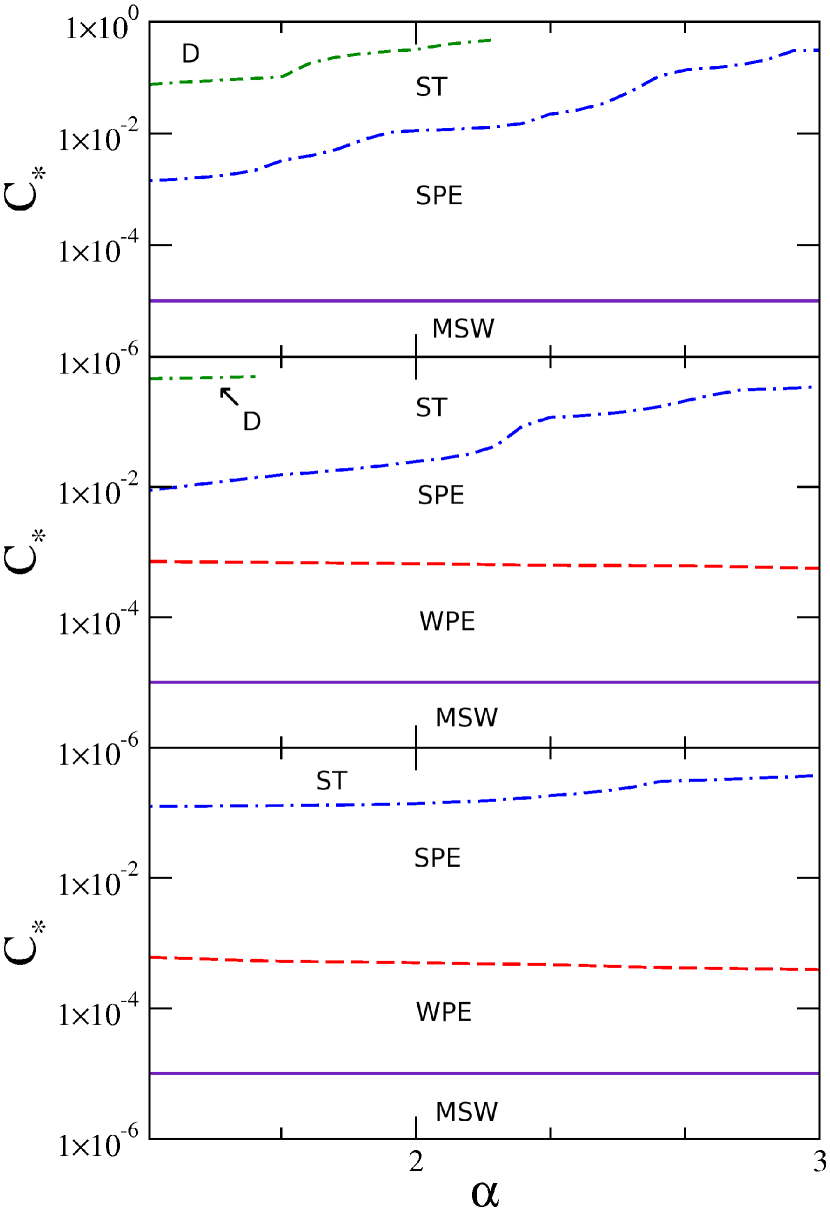
The two most important factors that determine the extent to which turbulence affects the neutrinos is the location of the turbulence in relation to the neutrino’s resonance densities and the turbulence amplitude. Turbulence effects are largest when the turbulence is located in the profile in the vicinity of the neutrino resonances (both L and H) because both effects depend upon the mixing matrix having both large diagonal and off-diagonal entries in the region where the turbulence is located and the MSW resonances are the locations where these entries are equal in magnitude. In this paper we have used a density profile at a fixed snapshot time and considered three different neutrino energies in order to demonstrate this dependence between the turbulence effects and MSW densities. Fixing the neutrino energy and changing the snapshot time would produce similar results. In figure (14) we show the regions of $C_{\star}$ and $\alpha$ where we find the various turbulence effects in the mixing between $\nu_{2}$ and $\nu_{3}$. To construct the figure we have extracted various contours of $\sigma_{23}$ from figure (5). For each energy we find no effect from turbulence when $C_{\star}\leq 10^{-5}$ so have set this as a lower limit in each case. For the $E=45\;{\rm MeV}$ neutrinos the boundary between the weak and saturated phase effects is taken to be where $\sigma_{23}=0.1$, the boundary between saturated phase effects and stimulated transitions as where $\sigma_{23}=0.2.$. For the $E=15\;{\rm MeV}$ neutrinos the boundary between the weak and saturated phase effects is taken to be where $\sigma_{23}=0.3$, and this same value of $\sigma_{23}$ forms the boundary between saturated phase effects and stimulated transitions. For the boundary between the depolarization region and the stimulated transitions we use $\sigma_{23}=0.25$. Finally, for the $E=5\;{\rm MeV}$ neutrinos we do not find a boundary between saturated and weak phase effects, the boundary between saturated phase effects and stimulated transitions is where $\sigma_{23}=0.1$ and depolarization is taken to occur when $\sigma_{23}\geq 0.2$. We caution the reader that these boundaries are somewhat fuzzy in the sense that on the boundaries the distributions are often mixtures and furthermore these values of $\sigma_{23}$ have no meaning in themselves. Let us use this figure to summarize what we have found.

If we optimize the location of the turbulence by careful selection of the profile, we find the stimulated transition effects appear in every mixing channel - even antineutrinos - when the turbulence amplitude exceeds $C_{\star}\gtrsim 1\%$. As one expects for the epoch chosen, the turbulence effects are strongest in the H resonant channel followed by the mixing in $\nu_{1}$-$\nu_{2}$ and $\bar{\nu}_{1}$-$\bar{\nu}_{2}$. The sensitivity of the H resonant channel at this epoch is largely the same for all three energies. The extent to which $\nu_{1}$-$\nu_{2}$ and $\bar{\nu}_{1}$-$\bar{\nu}_{2}$ are affected at this epoch does depend upon the neutrino energy because of the difference of the relation between the turbulent densities and the L resonance for different energies. Thus, at this epoch, we see lower energies affected by turbulence to a greater degree than higher energies due to the greater coupling between the states $\nu_{1}$ and $\nu_{2}$. But even though stimulated transition effects may be present, the neutrinos do not always exhibit a dependence upon the turbulence power spectral index because stimulated transitions possess a strong limit of depolarization and a weak limit. In the strong limit no $\alpha$ dependence is found because the distributions of the transition probabilities are depolarized, either two or three flavor; in the weak limit the distributions are found to be exponential and are sensitive to $\alpha$. The boundary between the two regimes shown in figure (14) depends upon $\alpha$ and the turbulence amplitude $C_{\star}$ with a greater proportion of depolarization at fixed $C_{\star}$ when the power spectrum is hardened.

Stimulated transitions occur when the product of turbulence amplitude and diagonal/off-diagonal mixing matrix elements is large. When this product is not above threshold the distorted phase effect of turbulence can become apparent. The boundary between stimulated transitions and phase effects is the dot-dashed line in figure (14). In fact, if we optimize the location of the turbulence then the sensitivity to $C_{\star}$ via the distorted phase effect can be extreme with turbulence amplitudes as small as $C_{\star}\sim 10^{-4}$ causing an effect. Note this amplitude is comparable with the amplitude of the density fluctuations in the progenitor 2011ApJ…733…78A ; 2015arXiv150302199C and furthermore the boundary between weak phase effects and the MSW only region in figure (14) varies with the epoch: at earlier epochs the boundary lies at much higher values of $C_{\star}$ because the turbulence is far from the H resonant region. Like stimulated transitions, the distorted phase effect has a strong and weak limit: in the strong limit the phase difference between discontinuities is distributed uniformly leading to arcsine distributions for the transition probabilities. When this occurs the parameters describing the arcsine distribution are determined by the jumps in the transition probabilities at the discontinuities and not the turbulence between them. For this reason the neutrinos are not affected by changes in the power spectral index. In the weak limit of the distorted phase effect the sensitivity to the power spectrum re-emerges due to the dominance of the long wavelength modes. Counter-intuitively, this sensitivity to the longest wavelengths means harder spectra have less of an effect than soft spectra for a given $C_{\star}$. This difference in the dependence upon $\alpha$ explains the downward slope of the boundary between strong and weak distorted phase effects in figure (14).

While the dependence of turbulence effects upon neutrino energy, turbulence amplitude, spectral index etc.  can be complicated, it is possible to use our results to piece together the expected evolution of the turbulence effects that neutrinos of a given energy will experience as a function of time. For neutrinos of a given energy there will be no sensitivity to the turbulence during the early phase of the burst signal because the turbulence is at densities far from the MSW resonances. This requirement that the turbulence be close to the resonance density is the reason there were no turbulence effects seen by Reid, Adams and Seunarine Reid when they put turbulence into the post-shock region in profiles appropriate for the accretion epoch. As the forward shock and turbulence move out into the star turbulence effects will start to appear. Initially these are due to distorted phase effects in the H resonance channel and, remarkably, the greater the spectral index $\alpha$ the greater the sensitivity to the turbulence of a given amplitude. As time progresses the distorted phase effects for a given neutrino energy will saturate to a limit where the sensitivity to $\alpha$ and $C_{\star}$ is lost. As time progresses further stimulated transition effects will begin to appear if the amplitude is greater than $C_{\star}\gtrsim 1\%$. Stimulated transitions appear first in the H resonance channel and again, initially, exhibit a sensitivity to $\alpha$ but now we find that smaller values of $\alpha$ lead to greater turbulence effects for a given $C_{\star}$. As time progresses further still, yet again that dependence upon $\alpha$ and $C_{\star}$ may disappear if the turbulence amplitude is sufficiently great to cause depolarization. If that occurs, turbulence effects will begin to appear in the mixing between other states most prominently between $\nu_{1}$-$\nu_{2}$ and in the antineutrinos in the $\bar{\nu}_{1}$-$\bar{\nu}_{2}$ channel. The mixing in $\nu_{1}$-$\nu_{2}$ and $\bar{\nu}_{1}$-$\bar{\nu}_{2}$ follows the same sequence as the mixing in the H resonant channel i.e.  it starts off as weak distorted phase effects sensitive to $\alpha$ and $C_{\star}$ that then saturates before stimulated transitions appear if $C_{\star}$ is sufficiently large. If stimulated transitions do start to affect the $\nu_{1}$-$\nu_{2}$ and $\bar{\nu}_{1}$-$\bar{\nu}_{2}$ evolution while mixing in the H resonant channel is still occurring then it is possible in a normal hierarchy to transition to three flavor depolarization if $\alpha$ is sufficiently small and $C_{\star}$ sufficiently large. Finally, as the turbulent region sweeps further out into the star, the turbulence effects will decrease in the H resonance channel and concentrate in the mixing between $\nu_{1}$-$\nu_{2}$ and $\bar{\nu}_{1}$-$\bar{\nu}_{2}$ which will then themselves eventually fade as the turbulence reaches the very outer edges of the star. The extent to which the turbulence effects at these late times are visible will depend upon the exact shape of the progenitor profile because the rapidly fading neutrino luminosity will make the statistics of detection very poor. This expected sequence of turbulence events allows us to answer our original question of whether the neutrinos exhibit sensitivity to the turbulence power spectrum. We conclude it indeed appears, in principal, there is sensitivity to the power spectral index in the signal from a Galactic supernova and further analyses along the lines of Borriello et al. 2013arXiv1310.7488B but for 3D simulations would be very welcome.