Remote sensing image classification exploiting multiple kernel learning

Abstract

We propose a strategy for land use classification which exploits Multiple Kernel Learning (MKL) to automatically determine a suitable combination of a set of features without requiring any heuristic knowledge about the classification task. We present a novel procedure that allows MKL to achieve good performance in the case of small training sets. Experimental results on publicly available datasets demonstrate the feasibility of the proposed approach.

I Introduction

The automatic classification of land use is of great importance for several applications in agriculture, forestry, weather forecasting, and urban planning. Land use classification consists in assigning semantic labels (such as urban, agricultural, residential etc.) to aerial or satellite images. The problem is closely related to that of land cover classification and differs from it mainly in the set of labels considered (forest, desert, open water etc.). In the past these problems have been often addressed by exploiting spectral analysis techniques to independently assign the labels to each pixel in the image [1]. Recently, several researchers experimented with image-based techniques consisting, instead, in extracting image features and in classifying them according to models obtained by supervised learning. Multiple features should be considered because the elements in the scene may appear at different scales and orientations and, due to variable weather and time of the day, also under different lighting conditions.

Sheng et al. designed a two-stage classifier that combines a set of complementary features [2]. In the first stage Support Vector Machines (SVM) are used to generate separate probability images using color histograms, local ternary pattern histogram Fourier (LTP-HF) features, and some features derived from the Scale Invariant Feature Transform (SIFT). To obtain the final result, these probability images are fused by the second stage of the classifier. Risojević et al. applied non-linear SVMs with a kernel function especially designed to be used with Gabor and Gist descriptors [3]. In a subsequent work, Risojević and Babić considered two features: the Enhanced Gabor Texture Descriptor (a global feature based on cross-correlations between subbands) and a local descriptor based on the SIFT. They identified the classes of images best suited for the two descriptors, and used this information to design a hierarchical approach for the final fusion [4]. Shao et al. [5] employed both non-linear SVMs and L1-regularized logistic regression in different classification stages to combine SIFT descriptors, shape features for image indexing, texture feature based on Local Binary Patterns (LBP) and a bag-of-colors signature.

In this paper, we propose a strategy for land use classification which exploits Multiple Kernel Learning (MKL) to automatically combine a set of features without requiring any heuristic knowledge about the classification task. One of the drawbacks of MKL is that it requires a large training set to select the features and to train the classifier simultaneously. In order to apply MKL to small training sets as well, we introduce a novel automatic procedure that produces candidate subsets of the available features before solving the optimization problem defined by the MKL framework. The proposed strategy exploits both features commonly used in scene classification as well as new features specially designed by the authors to cope with the land use classification problem. We evaluated our proposal on two data sets: the Land use data set of aerial images [6], and a data set of satellite images obtained from the Google Earth service [7]. We compared our framework with others from the state of the art. The results show that the proposed framework performs better than other methods when the training set is small.

II Proposed classification scheme

Multiple Kernel Learning (MKL) is a powerful machine learning tool which allows, in the framework of Support Vector Machines (SVM), to automatically obtain a suitable combinations of several kernels over several features (therefore selecting the features as well) [8, 9, 10, 11, 12]. We evaluated the MKL framework as proposed by Sonnenburg et al. [13] in the case of small size of the training set (results are detailed in the experimental section). We observed that dense mixtures of kernels can fit real data better than sparse mixtures but also that both sparse and non sparse solutions do not outperform other trivial baselines solutions such as those proposed by Risojević and et al. [4].

To improve the results in the case of small training sets, we introduce a novel heuristic procedure that automatically selects candidate subsets of the available combinations of features and kernels before solving the MKL optimization problem.

II-A Multiple Kernel Learning

Support Vector Machines exploit the ‘kernel trick’ to build non-linear binary classifiers. Given a feature vector $\mathbf{x}$, the predicted class $y$ (either $-1$ or $+1$) depends on a kernel $k$:

$$y=\mathrm{sign}(b+\sum_{i=1}^{N}\alpha_{i}y_{i}k(\mathbf{x},\mathbf{x}_{i})),$$ (1)

where $(\mathbf{x}_{i},y_{i})$ are the features/label pairs forming the training set. The parameters $b$ and $\alpha_{i}$ are determined during the training procedure, which consists in solving the following quadratic optimization problem:

$$\min_{\mathbf{\alpha}}\frac{1}{2}\sum_{i=1}^{N}\sum_{j=1}^{N}\alpha_{i}\alpha_{j}y_{i}y_{j}k(\mathbf{x}_{i},\mathbf{x}_{j})-\sum_{i=1}^{N}\alpha_{i},$$ (2)

under the constraints $\sum_{i}\alpha_{i}y_{i}=0$ and $0\leq\alpha_{i}\leq C$ (for a set value of the penalization parameter $C$). Beside the linear kernel ($k(\mathbf{x}_{1},\mathbf{x}_{2})=\mathbf{x}_{1}^{T}\cdot\mathbf{x}_{2}$), other popular kernels are the Gaussian RBF ($k(\mathbf{x}_{1},\mathbf{x}_{2})=\exp(-\gamma\|\mathbf{x}_{1}-\mathbf{x}_{2}\|^{2})$) and the $\chi^{2}$ kernel ($k(\mathbf{x}_{1},\mathbf{x}_{2})=\exp(-\gamma\sum_{j}\frac{(x_{1j}-x_{2j})^{2}}{x_{1j}+x_{2j}})$) both depending on an additional parameter $\gamma$.

The choice of the kernel function is very important since it implicitly defines the metric properties of the feature space. Multiple Kernel Learning (MKL) is an extension of Support Vector Machines (SVMs) that combines several kernels. It represents an appealing strategy when dealing with multiple feature vectors $\mathbf{x}=\langle\mathbf{x}^{(1)},\mathbf{x}^{(2)},\dots,\mathbf{x}^{(F)}\rangle$ and with multiple kernel functions $k_{1}^{(f)},k_{2}^{(f)},\dots,k_{M}^{(f)}$ for each feature. In MKL, the kernel function used in (1) is a linear combination of these $F\times M$ kernels

$$k_{comb}(\mathbf{x},\mathbf{x}_{i})=\sum_{f=1}^{F}\sum_{j=1}^{M}\beta^{(f)}_{j}k_{j}^{(f)}(\mathbf{x}^{(f)},{\bf x}_{i}^{(f)}).$$ (3)

The weights $\beta^{(f)}_{j}\geq 0$ are considered as additional parameters to be found when solving the optimization problem (2) with the inclusion of the new constraint $\sum_{f}\sum_{j}\beta^{(f)}_{j}=1$.

The first approaches to MKL aimed at finding sparse mixtures of kernels with the introduction of $l_{1}$ regularization for the weights of the combination. For instance, Lanckriet et al. induced the sparsity by imposing an upper bound to the trace of $k$ [14]. The resulting optimization was computationally too expensive for large scale problems [15]. Moreover, the use of sparse combinations of kernels rarely demonstrated to outperform trivial baselines in practical applications.

Sonnenburg et al. introduced an efficient strategy for solving $l_{p}$-regularized MKL with arbitrary norms, $p\geq 1$ [13, 15]. The algorithm they proposed allows to estimate optimal weights and SVM parameters simultaneously by iterating training steps of a standard SVM [13]. This strategy allows both sparse ($p=1$) and non-sparse ($p>1$) solutions (for the non-sparse case the constraint on the weights must be changed to $\sum_{f}\sum_{j}\left(\beta_{j}^{(f)}\right)^{p}=1$).

In the case of small training sets, plain SVMs may outperform MKL. This fact mostly depends on the increased number of parameters that have to be set during training, and is particularly evident when there are many features and kernels.

II-B Heuristic MKL

We introduce, here, a novel heuristic approach to MKL that finds sparse mixtures of kernels without imposing the sparsity condition ($p=1$). Using a small number of kernels is very important in the case of small training sets because it reduces the number of parameters to be learned and, consequently, limits the risk of overfitting the training data. In fact, using all the available kernels is usually worse than using a small selection of good kernels. Sparsity could be enforced by constraining to be zero a subset of the coefficients of the kernels before solving the $l_{2}$ regularized optimization problem. The optimal solution could be found by considering all the $2^{F\times M}$ possible subsets. However, this approach would easily result intractable even for relatively small numbers of feature vectors ($F$) and kernels ($M$). A tractable greedy solution would consist in selecting one kernel at a time on the basis of its individual merit. This approach, instead, would fail to capture most of the interactions among the kernels.

Our heuristic strategy deals with the limitations of the greedy algorithm, without resulting intractable as the exhaustive search. Briefly, It consists in the automatic selection of a small number of kernels (one for each feature vector) and in an iterative augmentation of such an initial selection. New kernels are not included only because of their performance in isolation, but they are chosen by taking into account how much they complement those that have been already selected. Since complementarity is more easily found across different features, at each iteration the algorithm considers for the inclusion at most one kernel for each feature vector. More in detail, the procedure is composed of four major steps. For each step the goodness of one or more sets of kernels is evaluated by training the MKL with $p=2$ and by a five-fold cross validation on the training set:

1. for each of the $F$ feature vectors and for each of the $M$ kernels, a classifier is trained and evaluated; the best kernel for each feature is then included in the initial selection $\mathcal{S}$;

2. the inclusion of each non-selected kernel is individually evaluated after its temporary addition to $\mathcal{S}$;

3. for each feature vector, the kernel corresponding to the largest improvement in step 2 is taken; these kernels are used to form a set $\mathcal{C}$ of candidate kernels. Features whose kernel does not improve the accuracy will remain without a candidate;

4. for each subsets of $\mathcal{C}$, its union with $\mathcal{S}$ is evaluated; the subset $\mathcal{B}^{*}$ corresponding to the largest improvement is permanently added to $\mathcal{S}$.

The steps 2–4 are repeated until the set of candidates $\mathcal{C}$ found in step 3 is empty (this would eventually happen since each step adds at least one kernel until no kernel improves the accuracy, or until all the kernels have been selected).

  {Step 1: initialization}

  $\mathcal{S}\leftarrow\emptyset$

  for $f\leftarrow 1$ to $F$ do

     $j^{*}\leftarrow\operatorname*{arg\,max}\limits_{j=1,\dots,M}\text{{\bf evaluate}}(\{k_{j}^{(f)}\}$)

     $\mathcal{S}\leftarrow\mathcal{S}\cup\{k_{j^{*}}^{(f)}\}$

  end for

  repeat

     {Steps 2 and 3: selection of the candidates}

     $\mathcal{C}\leftarrow\emptyset$

     for $f\leftarrow 1$ to $F$ do

        $\mathcal{T}^{(f)}\leftarrow\{k_{1}^{(f)},\dots,k_{M}^{(f)}\}\setminus\mathcal{S}$

        if $\mathcal{T}^{(f)}\neq\emptyset$ then

           $j^{*}\leftarrow\operatorname*{arg\,max}\limits_{j:k_{j}^{(f)}\in\mathcal{T}^{(f)}}\text{{\bf evaluate}}(\mathcal{S}\cup\{k_{j}^{(f)}\})$

           $\mathcal{C}\leftarrow\mathcal{C}\cup\{k_{j^{*}}^{(f)}\}$

        end if

     end for

     {Step 4: selection of the best set of kernels}

     $\mathcal{B}^{*}\leftarrow\operatorname*{arg\,max}\limits_{\mathcal{B}\subseteq\mathcal{C}}\text{{\bf evaluate}}(\mathcal{S}\cup\mathcal{B})$

     $\mathcal{S}\leftarrow\mathcal{S}\cup\mathcal{B}^{*}$

  until $\mathcal{B}^{*}=\emptyset$

  return  $\mathcal{S}$

Figure 1: The proposed heuristic: the procedure selects a subset $\mathcal{S}$ of the given kernels $\{k_{j}^{(f)}\}_{j=1\dots M,f=1\dots F}$. Starting from the set of the best kernels for each feature, a sequence of iterations selects additional kernels. In each iteration a set $\mathcal{C}$ of candidates is formed by taking up to one kernel for each feature vector. Then the best subset $\mathcal{B}^{*}$ of $\mathcal{C}$ is added to $\mathcal{S}$. The procedure continues until $\mathcal{B}^{*}$ is empty. The subroutine evaluate performs a five-fold cross validation on the training set to estimate the goodness of a set of kernels.

The whole procedure is detailed in the pseudo-code reported in Fig. 1. Step 4 requires the evaluation of up to $2^{F}-1$ combinations of candidates, and that step is repeated up to $M\times F$ times (since at least one kernel is added at each iteration). Therefore, in the worst case the number of trained classifiers is $O(F\times M\times 2^{F})$. Such a number can be kept manageable if the number of features $F$ is reasonable. As an example, in the setup used in our experiments $F=4$ and $M=9$ therefore the number of classifiers is less than $4\times 9\times 2^{4}=576$, which is several orders of magnitude less than the $2^{4\times 9}=6.87\times 10^{10}$ combinations required by the brute force strategy. As rough indicator consider that on 10% of the 19-class dataset described in the next section, the training with our strategy set required about 45 minutes on a standard PC.

III Experimental evaluation

To assess the merits of the classifier designed according to our proposal, we compared it with other approaches in the state of the art on two data sets. For all the experiments, the “one versus all” strategy is used to deal with multiple classes. The evaluation includes:

• image features: we evaluated several types of image features and their concatenation using SVMs with different kernels (linear, RBF and $\chi^{2}$);

• MKL: we evaluated three versions of MKL ($p=1$, $p=1.25$, $p=2$ and the proposed strategy); as alternative heuristic for the initialization of MKL we considered the kernel alignement method proposed by Tuia et al. [10] with and without centered kernels [16];

• other approaches in the state of the art: we evaluated the method proposed by Risojević et al. [4] (‘metalearner’, with both the features described in the original paper and the features described in this paper).

III-A Data and image features

21-Class Land-Use Dataset

this is a dataset of images of 21 land-use classes selected from aerial orthoimagery with a pixel resolution of one foot [6]. For each class, 100 RGB images at $256\times 256$ are available. These classes contain a variety of spatial patterns, some homogeneous with respect to texture, some homogeneous with respect to color, others not homogeneous at all.

19-Class Satellite Scene

this dataset consists of 19 classes of satellite scenes collected from Google Earth (Google Inc.). Each class has about 50 RGB images, with the size of $600\times 600$ pixels [7, 17]. The images of this dataset are extracted from very large satellite images on Google Earth.

We considered four types of image features ($F=4$): two of them have been taken from the state of the art and have been chosen because of the good performance that are reported in the literature. The other two features have been specially designed, here, to complement the others.

III-A1 Bag of SIFT

we considered SIFT [18] descriptors computed on the intensity image and quantized into a codebook of 1096 “visual words”. This codebook has been previously built by $k$-means clustering the descriptors extracted from more than 30,000 images. To avoid unwanted correlations with the images used for the evaluation, we built the codebook by searching general terms on the flickr web service and by downloading the returned images. The feature vector is a histogram of 1096 visual words.

III-A2 Gist

these are features computed from a wavelet decomposition of the intensity image [19]. Each image location is represented by the output of filters tuned to different orientations and scales. This representation is then downsampled to $4\times 4$ pixels. We used eight orientations and four scales thus, the dimensionality of the feature vector is $8\times 4\times 16=512$.

TABLE I: Performance comparisons on the two datasets.

		% training images per class (21-class data set)
Features	Kernel	5	10	20	50	80	90
Bag of SIFT	$\chi^{2}$	51.89 ($\pm$1.73)	59.13 ($\pm$1.53)	66.09 ($\pm$1.11)	76.80 ($\pm$1.11)	77.42 ($\pm$1.99)	85.45 ($\pm$2.83)
Bag of LBP	$\chi^{2}$	42.07 ($\pm$2.35)	50.39 ($\pm$1.44)	59.21 ($\pm$1.26)	76.51 ($\pm$1.16)	77.18 ($\pm$1.83)	74.81 ($\pm$2.79)
GIST	$\chi^{2}$	38.62 ($\pm$1.74)	45.62 ($\pm$1.44)	53.73 ($\pm$1.20)	67.96 ($\pm$1.30)	68.53 ($\pm$1.73)	67.35 ($\pm$2.63)
LBP of moments	RBF	24.41 ($\pm$1.47)	29.58 ($\pm$1.30)	34.54 ($\pm$1.05)	44.62 ($\pm$1.20)	45.26 ($\pm$2.13)	59.49 ($\pm$3.24)
Concatenation	RBF	58.25 ($\pm$2.21)	69.19 ($\pm$1.56)	77.32 ($\pm$1.23)	85.44 ($\pm$1.04)	88.91 ($\pm$1.23)	89.41 ($\pm$1.81)
	$\chi^{2}$	58.05 ($\pm$2.21)	68.58 ($\pm$1.44)	76.97 ($\pm$1.21)	85.09 ($\pm$0.95)	88.33 ($\pm$1.31)	88.55 ($\pm$1.92)
Metalearner [4] (original features)	Ridge regression C	56.05 ($\pm$2.09)	70.30 ($\pm$1.64)	79.99 ($\pm$1.21)	88.45 ($\pm$0.90)	91.59 ($\pm$1.20)	91.98 ($\pm$1.74)
	RBF SVM	48.58 ($\pm$2.63)	64.91 ($\pm$2.13)	79.16 ($\pm$1.23)	89.28 ($\pm$0.86)	92.52 ($\pm$1.07)	92.98 ($\pm$1.64)
	RBF ridge regr.	51.77 ($\pm$2.61)	65.52 ($\pm$2.46)	80.26 ($\pm$1.18)	88.62 ($\pm$1.01)	91.76 ($\pm$1.13)	92.23 ($\pm$1.72)
	RBF ridge regr. C	54.92 ($\pm$2.13)	69.10 ($\pm$1.94)	79.79 ($\pm$1.20)	89.04 ($\pm$0.93)	92.16 ($\pm$1.11)	92.57 ($\pm$1.71)
Metalearner [4]	Ridge regression	40.25 ($\pm$2.76)	59.88 ($\pm$1.83)	71.36 ($\pm$1.32)	83.04 ($\pm$1.14)	87.79 ($\pm$1.31)	88.66 ($\pm$1.99)
	RBF SVM	38.75 ($\pm$2.98)	52.62 ($\pm$2.39)	66.35 ($\pm$1.77)	82.72 ($\pm$1.23)	88.44 ($\pm$1.43)	89.21 ($\pm$1.79)
	RBF ridge regr.	42.93 ($\pm$2.71)	58.22 ($\pm$2.28)	71.78 ($\pm$1.49)	83.68 ($\pm$1.11)	88.24 ($\pm$1.25)	88.81 ($\pm$1.92)
	RBF ridge regr. C	39.41 ($\pm$2.37)	59.53 ($\pm$1.91)	71.52 ($\pm$1.35)	83.47 ($\pm$1.06)	87.85 ($\pm$1.35)	88.58 ($\pm$1.98)
Kernel Alignment [10]	Linear, RBF, $\chi^{2}$	61.16 ($\pm$1.79)	71.42 ($\pm$1.32)	77.65 ($\pm$1.03)	84.23 ($\pm$0.95)	86.88 ($\pm$1.39)	87.61 ($\pm$2.13)
Kernel Alignment [10] $+$ Kernel Cent.	Linear, RBF, $\chi^{2}$	61.59 ($\pm$1.90)	70.77 ($\pm$1.70)	79.10 ($\pm$1.13)	86.56 ($\pm$0.91)	90.07 ($\pm$1.29)	90.45 ($\pm$1.86)
MKL ($p=1$) [13]	Linear, RBF, $\chi^{2}$	55.91 ($\pm$2.24)	68.28 ($\pm$1.72)	78.34 ($\pm$1.16)	87.74 ($\pm$0.82)	90.50 ($\pm$1.35)	91.20 ($\pm$1.74)
MKL ($p=1.25$) [13]	Linear, RBF, $\chi^{2}$	58.31 ($\pm$2.13)	69.42 ($\pm$1.69)	78.10 ($\pm$1.20)	86.71 ($\pm$0.82)	89.70 ($\pm$1.31)	90.34 ($\pm$1.76)
MKL ($p=2$) [13]	Linear, RBF, $\chi^{2}$	59.87 ($\pm$1.96)	70.29 ($\pm$1.59)	78.12 ($\pm$1.14)	86.06 ($\pm$0.84)	89.03 ($\pm$1.32)	89.69 ($\pm$1.82)
Proposed MKL + Kernel Normalization	Linear, RBF , $\chi^{2}$	64.07 ($\pm$1.57)	74.00 ($\pm$1.50)	81.00 ($\pm$1.18)	88.50 ($\pm$0.83)	91.30 ($\pm$1.22)	91.64 ($\pm$1.94)
Proposed MKL	Linear, RBF, $\chi^{2}$	65.20 ($\pm$1.57)	74.57 ($\pm$1.45)	81.11 ($\pm$1.14)	88.86 ($\pm$0.90)	91.84 ($\pm$1.29)	92.31 ($\pm$1.78)

		% training images per class (19-class data set)
Features	Kernel	5	10	20	50	80	90
Bag of SIFT	$\chi^{2}$	49.94 ($\pm$2.91)	61.71 ($\pm$1.96)	71.03 ($\pm$1.67)	80.32 ($\pm$1.73)	84.27 ($\pm$2.11)	85.45 ($\pm$3.26)
LBP	$\chi^{2}$	39.69 ($\pm$2.58)	46.24 ($\pm$2.18)	56.61 ($\pm$1.82)	68.88 ($\pm$1.79)	74.15 ($\pm$2.94)	74.81 ($\pm$3.64)
GIST	$\chi^{2}$	34.87 ($\pm$2.71)	44.87 ($\pm$2.31)	53.44 ($\pm$1.59)	62.03 ($\pm$1.73)	66.31 ($\pm$2.73)	67.35 ($\pm$3.65)
LBP of moments	RBF	20.43 ($\pm$1.85)	30.01 ($\pm$3.39)	46.86 ($\pm$2.25)	50.12 ($\pm$1.89)	58.11 ($\pm$2.65)	59.49 ($\pm$4.34)
Concatenation	RBF	63.28 ($\pm$2.62)	78.28 ($\pm$1.93)	86.66 ($\pm$1.39)	93.17 ($\pm$1.08)	95.11 ($\pm$1.47)	95.90 ($\pm$1.88)
	$\chi^{2}$	58.03 ($\pm$3.25)	76.67 ($\pm$2.13)	86.08 ($\pm$1.61)	93.26 ($\pm$1.22)	95.68 ($\pm$1.35)	96.01 ($\pm$1.99)
Metalearner [4] (original features)	Ridge regression C	49.61 ($\pm$4.24)	77.03 ($\pm$2.23)	84.54 ($\pm$1.73)	92.56 ($\pm$1.01)	94.93 ($\pm$1.52)	95.57 ($\pm$1.93)
	RBF SVM	41.22 ($\pm$5.06)	73.14 ($\pm$2.67)	85.78 ($\pm$2.01)	95.47 ($\pm$0.88)	97.22 ($\pm$1.19)	97.92 ($\pm$1.27)
	RBF ridge regr.	44.52 ($\pm$5.01)	76.69 ($\pm$2.42)	87.24 ($\pm$1.84)	94.62 ($\pm$1.06)	96.98 ($\pm$1.33)	97.60 ($\pm$1.51)
	RBF ridge regr. C	44.40 ($\pm$3.95)	76.13 ($\pm$2.40)	85.10 ($\pm$1.93)	93.71 ($\pm$1.20)	95.69 ($\pm$1.44)	96.05 ($\pm$1.82)
Metalearner [4]	Ridge regression	43.44 ($\pm$4.20)	58.89 ($\pm$2.88)	77.05 ($\pm$2.08)	90.02 ($\pm$1.23)	93.20 ($\pm$1.51)	93.67 ($\pm$2.34)
	RBF SVM	49.74 ($\pm$3.94)	69.86 ($\pm$2.72)	83.16 ($\pm$1.72)	94.80 ($\pm$1.07)	96.71 ($\pm$1.12)	97.10 ($\pm$1.72)
	RBF ridge regr.	53.36 ($\pm$3.65)	75.70 ($\pm$2.24)	88.06 ($\pm$1.47)	95.08 ($\pm$1.00)	96.92 ($\pm$1.09)	97.01 ($\pm$1.73)
	RBF ridge regr. C	34.81 ($\pm$4.28)	51.88 ($\pm$3.45)	77.70 ($\pm$2.07)	90.55 ($\pm$1.29)	93.50 ($\pm$1.48)	94.02 ($\pm$2.48)
Kernel Alignment [10]	Linear, RBF, $\chi^{2}$	58.27 ($\pm$3.12)	74.11 ($\pm$1.84)	82.70 ($\pm$1.55)	93.65 ($\pm$1.03)	94.99 ($\pm$1.40)	95.98 ($\pm$1.80)
Kernel Alignment [10] $+$ Kernel Cent.	Linear, RBF, $\chi^{2}$	61.50 ($\pm$3.06)	78.40 ($\pm$1.94)	87.96 ($\pm$1.48)	94.62 ($\pm$0.97)	96.20 ($\pm$1.15)	96.74 ($\pm$1.63)
MKL ($p=1$) [13]	Linear, RBF, $\chi^{2}$	53.83 ($\pm$3.72)	76.11 ($\pm$2.30)	87.96 ($\pm$1.42)	94.78 ($\pm$0.92)	96.50 ($\pm$1.21)	96.75 ($\pm$1.67)
MKL ($p=1.25$) [13]	Linear, RBF, $\chi^{2}$	58.67 ($\pm$3.43)	77.34 ($\pm$2.09)	87.61 ($\pm$1.46)	94.53 ($\pm$0.89)	96.31 ($\pm$1.12)	96.70 ($\pm$1.73)
MKL ($p=2$) [13]	Linear, RBF, $\chi^{2}$	61.88 ($\pm$3.01)	78.49 ($\pm$2.00)	87.64 ($\pm$1.48)	94.21 ($\pm$0.93)	95.95 ($\pm$1.19)	96.53 ($\pm$1.86)
Proposed MKL + Kernel Normalization	Linear, RBF, $\chi^{2}$	69.73 ($\pm$2.67)	83.45 ($\pm$1.63)	90.39 ($\pm$1.23)	95.33 ($\pm$0.78)	96.60 ($\pm$1.01)	96.90 ($\pm$1.53)
Proposed MKL	Linear, RBF, $\chi^{2}$	70.20 ($\pm$2.54)	84.05 ($\pm$1.67)	90.80 ($\pm$1.26)	95.73 ($\pm$0.85)	96.83 ($\pm$1.04)	97.36 ($\pm$1.48)

III-A3 Bag of dense LBP

local binary patterns are calculated on square patches of size $w\times w$ that are extracted as a dense grid from the original image. The final descriptor is obtained as a bag of such LBP patches obtained from a previously calculated dictionary. As for the SIFT, the codebook has been calculated from a set of thousands of generic scene images. Differently from SIFT, here we used a grid sampling with a step of 16 pixels. Note that this descriptor has been computed separately on the RGB channels and then concatenated. We have chosen the LBP with a circular neighbourhood of radius 2 and 16 elements, and 18 uniform and rotation invariant patterns. We set $w=16$ and $w=30$ for the 21-classes and 19-classes respectively. The size of the codebook, as well as the size of the final feature vector, is 1024.

III-A4 LBP of dense moments

the original image is divided in a dense grid of $N$ square patches of size $w\times w$. The mean and the standard deviation of each patch is computed for the red, green and blue channels. Finally, the method computes the LBP of each matrix and the final descriptor is then obtained by concatenating the two resulting LBP histograms of each channel. We have chosen the LBP with a circular neighbourhood of radius 2 and 16 elements, and 18 uniform and rotation invariant patterns. We set $w=16$ and $w=30$ for the 21-classes and 19-classes respectively. The final dimensionality of the feature vector is $3\times(18+18)=108$.

III-B Experiments

For each dataset we used training sets of different sizes. More in detail, we used 5, 10, 20, 50, 80 and 90% of the images for training the methods, and the rest for their evaluation. To make the results as robust as possible, we repeated the experiments 100 times with different random partitions of the data (available on the authors’ web page).

In the experiments for single kernel we used the parallel version of LIBSVM  [20]. For MKL we used the algorithm proposed by Sonnenburg et al. [15][13] that is part of the SHOGUN toolbox. For both single and multiple kernel experiments, we considered the linear, Gaussian RBF and $\chi^{2}$ kernel functions. In the case of single kernel the parameter $\gamma$ has been found by the standard SVM model selection procedure; for MKL we used the values $\gamma=\{10,1,0.1,0.01\}$ and $\gamma=\{3,2,1,0.5\}$ for the Gaussian RBF and $\chi^{2}$ kernels respectively (chosen taking into account the average Euclidean and $\chi^{2}$ distances of the features; more values could be used at the expenses of an increase in computation time). The coefficient $C$ has been chosen among the values $\{0.1,1,2,3,4,5\}$. For experiments with the metalearner we used the code kindly provided by the authors without any modifications. For all the other methods, before the computation of the kernels, all the feature vectors, have been $L_{2}$ normalized. For the standard MKL and the heuristic MKL we also normalized all the kernels by the standard deviation in the Hilbert’s space.

Table I reports the results obtained. Among single features, bag of SIFT obtained the highest accuracy, with the exception of the case of a large training set for the 21-class dataset where the best feature is the bag of LBP (for the sake of brevity, only the results obtained with the best kernel are reported). Regardless the size of the training set, the concatenation of the feature vectors improved the results. In fact, features such as the LBP of moments that resulted weak when used alone, demonstrated to be useful when combined with other features.

On the 21-class dataset advanced combination strategies, such as the metalearners proposed in [4] or the MKL as defined in [13], performed better than simple concatenations. However, this is not true for the 19-class dataset. The metalearner works better with its own original features than with our features (this could be due to the fact that these features were based on a codebook defined on the same dataset).

The proposed MKL strategy, in the case of small training sets, outperformed all the other methods considered. More in detail, when trained on 10% of the 21-class dataset the accuracy of our method was by at least 3% better than the accuracy of the other strategies. Similarly, for the 10% of the 19-class dataset, our method was the only one with an accuracy higher than 80%. Even larger improvements have been obtained when using 5% of the data for training. The improvement obtained in the case of small training sets is statistically significant as it passed a two-tailed paired t-test with a confidence level of 95%.

The weights assigned by the heuristic MKL are quite stable across the different classes (see Figure 2). Figure 3 shows the classification accuracy as a function of the number of iterations of the proposed method when 10% of images are used for training. According to the plot most of the improvement with respect to standard MKL is obtained after just a couple of iterations.

IV Conclusions

In land use classification scenes may appear at different scales, orientations and lighting conditions. Therefore, multiple features must be combined in order to obtain good performance. In this paper we presented a classification strategy that improves MKL by making it suitable for small training sets. Experimental results on two public land use datasets shown that our method performs better than the other alternatives considered. We believe that our approach could be applied to other image classification tasks. In particular, we expect that it may be successful in those cases where few training data are available and, at the same time, multiple features are needed.

Our MKL strategy may be applied to any set of features, future works will address a deeper investigation about feature design. It has been demonstrated that kernel normalization techniques can significantly influence the performance of MKL [13], we will also investigate how to effectively exploit these techniques within our MKL strategy.

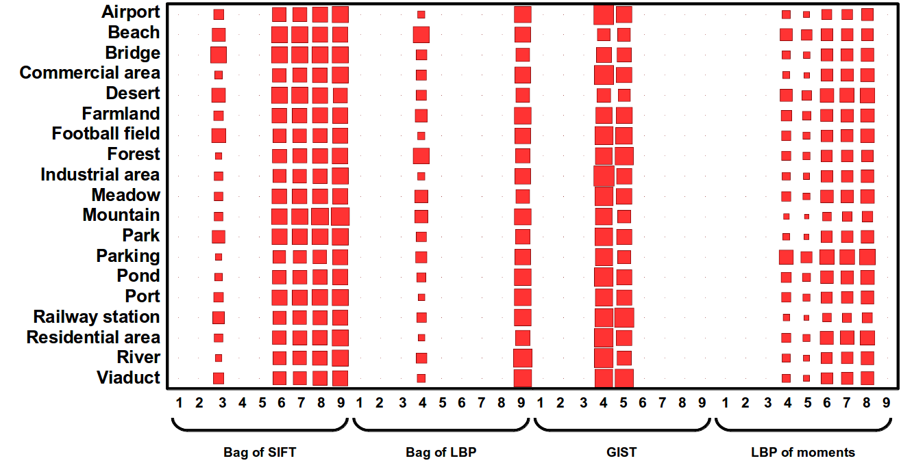
Figure 2: Weights selected by the heuristic MKL when trained on the 19-class data set. Numbers at the bottom indicate kernels: 1 for linear, 2–5 for RBFs at different $\gamma$, 6–9 for $\chi^{2}$s at different $\gamma$. The size of the squares is proportional to the weights. In order to make the weights comparable, we preprocessed the kernels with the normalization scheme proposed by Zien and Ong [21].

Figure 3: Accuracy of the proposed MKL varying the number of iterations, on the 19-class data set with 10% of training images. The performance of standard MKL ($p=2$) is reported for comparison.

References

- [1] J. Campbell, Introduction to remote sensing. CRC Press, 2002.
- [2] G. Sheng, W. Yang, T. Xu, and H. Sun, “High-resolution satellite scene classification using a sparse coding based multiple feature combination,” Int’l J. of Remote Sensing, vol. 33, no. 8, pp. 2395–2412, 2012.
- [3] V. Risojević, S. Momić, and Z. Babić, “Gabor descriptors for aerial image classification,” in Adap. & Nat. Comp. Alg., 2011, pp. 51–60.
- [4] V. Risojevic and Z. Babic, “Fusion of global and local descriptors for remote sensing image classification,” Geoscience and Remote Sensing Letters, vol. 10, no. 4, pp. 836–840, 2013.
- [5] W. Shao, W. Yang, G.-S. Xia, and G. Liu, “A hierarchical scheme of multiple feature fusion for high-resolution satellite scene categorization,” in Computer Vision Systems, 2013, pp. 324–333.
- [6] Y. Yang and S. Newsam, “Bag-of-visual-words and spatial extensions for land-use classification,” in Proc. of the Int’l Conf. on Advances in Geographic Information Systems, 2010, pp. 270–279.
- [7] D. Dai and W. Yang, “Satellite image classification via two-layer sparse coding with biased image representation,” Geoscience and Remote Sensing Letters, vol. 8, no. 1, pp. 173–176, 2011.
- [8] G. R. Lanckriet, T. De Bie, N. Cristianini, M. I. Jordan, and W. S. Noble, “A statistical framework for genomic data fusion,” Bioinformatics, vol. 20, no. 16, pp. 2626–2635, 2004.
- [9] S. Sonnenburg, G. Rätsch, C. Schäfer, and B. Schölkopf, “Large scale multiple kernel learning,” J. Mach. Learn. Res., vol. 7, pp. 1531–1565, 2006.
- [10] D. Tuia, G. Camps-Valls, G. Matasci, and M. Kanevski, “Learning relevant image features with multiple-kernel classification,” IEEE Trans. on Geosci. Remote Sens., vol. 48, no. 10, pp. 3780–3791, 2010.
- [11] N. Subrahmanya and Y. C. Shin, “Sparse multiple kernel learning for signal processing applications,” IEEE Trans. Pattern Anal. Mach. Intell., vol. 32, no. 5, pp. 788–798, 2010.
- [12] Y. Gu, C. Wang, D. You, Y. Zhang, S. Wang, and Y. Zhang, “Representative multiple kernel learning for classification in hyperspectral imagery,” IEEE Trans. on Geosci. Remote Sens., vol. 50, pp. 2852–2865, 2012.
- [13] M. Kloft, U. Brefeld, S. Sonnenburg, and A. Zien, “Lp-norm multiple kernel learning,” J. Mach. Learn. Res., vol. 12, pp. 953–997, 2011.
- [14] G. R. G. Lanckriet, N. Cristianini, P. Bartlett, L. E. Ghaoui, and M. I. Jordan, “Learning the kernel matrix with semidefinite programming,” J. Mach. Learn. Research, vol. 5, pp. 27–72, 2004.
- [15] M. Kloft, U. Brefeld, S. Sonnenburg, P. Laskov, K.-R. Müller, and A. Zien, “Efficient and accurate lp-norm multiple kernel learning,” in Advances in NIPS, vol. 22, no. 22, 2009, pp. 997–1005.
- [16] B. Schölkopf, A. Smola, and K.-R. Müller, “Kernel principal component analysis,” in ICANN’97. Springer, 1997, pp. 583–588.
- [17] G.-S. Xia, W. Yang, J. Delon, Y. Gousseau, H. Sun, H. Maître et al., “Structural high-resolution satellite image indexing,” in ISPRS TC VII Symposium-100 Years ISPRS, vol. 38, 2010, pp. 298–303.
- [18] D. Lowe, “Distinctive image features from scale-invariant keypoints,” Int’l J. Computer Vision, vol. 60, no. 2, pp. 91–110, 2004.
- [19] A. Oliva and A. Torralba, “Modeling the shape of the scene: A holistic representation of the spatial envelope,” Int’l J. Computer Vision, vol. 42, no. 3, pp. 145–175, 2001.
- [20] F. Li, J. Carreira, and C. Sminchisescu, “Object recognition as ranking holistic figure-ground hypotheses,” in IEEE CVPR, 2010.
- [21] A. Zien and C. S. Ong, “Multiclass multiple kernel learning,” in Proc. of the Int’l Conf. on Mach. learning, 2007, pp. 1191–1198.