On the Influence of Graph Density on Randomized Gossiping

Abstract

Information dissemination is a fundamental problem in parallel and distributed computing. In its simplest variant, known as the broadcasting problem, a single message has to be spread among all nodes of a graph. A prominent communication protocol for this problem is based on the so-called random phone call model (Karp et al., FOCS 2000). In each step, every node opens a communication channel to a randomly chosen neighbor, which can then be used for bi-directional communication. In recent years, several efficient algorithms have been developed to solve the broadcasting problem in this model.

Motivated by replicated databases and peer-to-peer networks, Berenbrink et al., ICALP 2010, considered the so-called gossiping problem in the random phone call model. There, each node starts with its own message and all messages have to be disseminated to all nodes in the network. They showed that any $O(\log n)$-time algorithm in complete graphs requires $\Omega(\log n)$ message transmissions per node to complete gossiping, with high probability, while it is known that in the case of broadcasting the average number of message transmissions per node is $O(\log\log n)$. Furthermore, they explored different possibilities on how to reduce the communication overhead of randomized gossiping in complete graphs.

It is known that the $O(n\log\log n)$ bound on the number of message transmissions produced by randomized broadcasting in complete graphs cannot be achieved in sparse graphs even if they have best expansion and connectivity properties. In this paper, we analyze whether a similar influence of the graph density also holds w.r.t. the performance of gossiping. We study analytically and empirically the communication overhead generated by gossiping algorithms w.r.t. the random phone call model in random graphs and also consider simple modifications of the random phone call model in these graphs. Our results indicate that, unlike in broadcasting, there seems to be no significant difference between the performance of randomized gossiping in complete graphs and sparse random graphs. Furthermore, our simulations illustrate that by tuning the parameters of our algorithms, we can significantly reduce the communication overhead compared to the traditional push-pull approach in the graphs we consider.

1 Introduction

1.1 Motivation

Information dissemination is a fundamental problem in parallel and distributed computing. Given a network, the goal is to spread one or several messages efficiently among all nodes of the network. This problem has extensively been analyzed in different communication models and on various graph classes. When talking about information dissemination, we distinguish between one-to-all communication called broadcasting and all-to-all communication called gossiping. Much of the work devoted to information dissemination refers to the broadcasting problem. That is, a distinguished node of the network possesses a piece of information, which has to be distributed to all nodes in the system. In gossiping, every node has its own piece of information, and all these messages must be distributed to all other nodes in the network. Efficient algorithms for gossiping are applied, e.g., in routing, maintaining consistency in replicated databases, multicasting, and leader election, see [8, 25, 33].

There are two main approaches to design efficient algorithms for broadcasting or gossiping. One way is to exploit the structural properties of the networks the protocols are deployed on to design efficient deterministic schemes [33]. While the resulting protocols are usually (almost) optimal, they are often not fault tolerant (note that there are also deterministic schemes, which have polylogarithmic running time on the graphs we consider and are highly robust, see [31]). Another approach is to design simple randomized algorithms, which are inherently fault tolerant and scalable. Prominent examples of such algorithms are based on the so-called random phone call model, which has been introduced by Demers et al. [16] and analyzed in detail by Karp et al. [34]. The algorithms in this model are synchronous, i.e., the nodes act in synchronous steps. In each step every node opens a communication channel to a randomly chosen neighbor. The channel can then be used for bi-directional communication to exchange messages between the corresponding nodes. It is assumed that the nodes may decide which messages to send (they are allowed to send none of their messages in some step), and are able to combine several messages to one single packet, which can then be sent through a channel. Clearly, one question is how to count the message complexity if several pieces of information are contained in such a packet; we will come back to this question later.

Karp et al. motivated their work with consistency issues in replicated databases, in which frequent updates occur. These updates must be disseminated to all nodes in the network to keep the database consistent. They analyzed the running time and number of message transmissions produced by so-called push and pull algorithms w.r.t. one single message in complete graphs. In order to determine the communication overhead, they counted the number of transmissions of this message through the links in the network. They argued that since updates occur frequently nodes have to open communication channels in each step anyway. Thus, the cost of opening communication channels amortizes over the total number of message transmissions.

Motivated by the application above, Berenbrink et al. considered the gossiping problem [5]. They assume that sending a packet through an open channel is counted once, no matter how many messages are contained in this packet. However, nodes may decide not to open a channel in a step, while opening a communication channel is also counted for the communication complexity. The first assumption is certainly unrealistic in scenarios, in which all original messages of the nodes have to be disseminated to all other nodes; although network coding might overcome the inpracticability of this assumption in certain applications (see e.g. [30]). On the other side, in the case of leader election, aggregate computation (e.g. computing the minimum or the average), or consensus the assumption above might be feasible, since then the size of the exchanged messages can asymptotically be bounded to the size of a single message.

The algorithms developed so far in the random phone call model use so-called push and pull transmissions. As described above, the nodes open communication channels to some (randomly) selected neighbors. If a message is sent from the node which called on a neighbor and initiated the communication, then we talk about a push transmission (w.r.t. that message). If the message is transmitted from the called node to the one that opened the channel, then we talk about a pull transmission.

Although the time complexity has extensively been analyzed on various networks in the past, the message complexity was mainly studied in complete graphs. The question is, whether the results known for complete graphs also hold in sparse networks with very good expansion and connectivity properties. Such networks naturally arise in certain real world applications such as peer-to-peer systems [11, 29]. In the case of broadcasting, it is known that the performance of push-pull algorithms in complete graphs cannot be achieved in random graphs of small or moderate degree [19]. This, however, seems not to be the case w.r.t. gossiping. As we show in this paper, concerning the number of message transmissions the performance of the algorithms developed in [5] can be achieved in random graphs as well. Regarding the impact of the graph density on the running time a similar study has been done by Fountoulakis et al. [24]. They showed that there is almost no difference between the running time of the push algorithm in complete graphs and random graphs of various degrees, as long as the expected degree is $\omega(\log n)$.

1.2 Related Work

A huge amount of work has been invested to analyze information dissemination in general graphs as well as some special network classes. We only concentrate here on randomized protocols which are based on the random phone call model. This model has been introduced by Demers et al. [16] along with a randomized algorithm that solves the problem of mutual consistency in replicated databases.

Many papers analyze the running time of randomized broadcasting algorithms that only use push transmissions. To mention some of them, Pittel [39] proved that in a complete graph a rumor can be distributed in $\log_{2}(n)+\ln(n)+\operatorname{O}\left(1\right)$ steps. Feige et al. [23] presented optimal upper bounds for the running time of this algorithm in various graph classes including random graphs, bounded degree graphs, and the hypercube.

In their paper, Karp et al. [34] presented an approach that requires only $\operatorname{O}\left(\log{n}\right)$ time and $\operatorname{O}\left(n\log\log{n}\right)$ message transmissions, with high probability, which is also shown to be asymptotically optimal. This major improvement is a consequence of their observation that an algorithm that uses only pull steps is inferior to the push approach as long as less than half of the nodes are informed. After that, the pull approach becomes significantly better. This fact is used to devise an algorithm that uses both, push and pull operations, along with a termination mechanism.

The random phone call model as well as some variants of it have also been analyzed in other graph classes. We mention here the work of Chierichetti et al. and Giakkoupis [14, 26] who related the running time of push-pull protocols to the conductance of a graph; or the work of Giakkoupis and Sauerwald [28, 27] on the relationship between push-pull and vertex expansion. To overcome bottlenecks in graphs with small conductance, Censor-Hillel and Shachnai used the concept of weak conductance in order to improve the running time of gossiping [12]. Earlier results related randomized information dissemination to random walks on graphs, see e.g. [37, 21]. Modifications of the random phone call model resulted in an improved performance of randomized broadcasting w.r.t. its communication complexity in random graphs [20] and its running time in the preferential attachment model [17]. The basic idea of these modifications is used in Section 4.

Randomized gossiping in complete graphs has been extensively studied by Berenbrink et al. [5]. In their paper, they provided a lower bound argument that proves $\operatorname{\Omega}\left(n\log{n}\right)$ message complexity for any $\operatorname{O}\left(\log{n}\right)$ time algorithm. This separation result marks a cut between broadcasting and gossiping in the random phone call model. Furthermore, the authors gave two algorithms at the two opposite points of the time and message complexity trade-off. Finally, they slightly modified the random phone call model to circumvent these limitations and designed a randomized gossiping protocol which requires $\operatorname{O}\left(\log{n}\right)$ time and $\operatorname{O}\left(n\log\log{n}\right)$ message transmissions.

Chen and Pandurangan [13] used gossiping algorithms for computing aggregate functions in complete graphs (see also [35]). They showed a lower bound of $\operatorname{\Omega}\left(n\log{n}\right)$ on the message complexity regardless of the running time for any gossiping algorithm. However, for this lower bound they assumed a model that is slightly weaker than the one used in this paper. In the main part of their paper, they presented an algorithm that performs gossiping in $\operatorname{O}\left(\log{n}\right)$ time using $\operatorname{O}\left(n\log\log{n}\right)$ messages by building certain communication trees. Furthermore, they also designed gossip protocols for general graphs. For all these algorithms, they assumed a communication model which is more powerful than the random phone call model.

Another interesting application of randomized gossiping is in the context of resilient information exchange [2]. Alistarh et al. proposed an algorithm with an optimal $\operatorname{O}\left(n\right)$ communication overhead, which can tolerate oblivious faults. For adaptive faults they provided a gossiping algorithm with a communication complexity of $\operatorname{O}\left(n\log^{3}n\right)$. Their model, however, is stronger than the random phone call model or some simple variants of it.

Random graphs first appeared in probabilistic proofs by Erdős and Rényi [22]. Much later, they were described in the works by Bender and Canfield [4], Bollobás [9] and Wormald [42, 41]. Aiello et al. generalized the classical random graph model introducing a method to generate and model power law graphs [1]. The properties of Erdős-Rényi graphs have been surveyed by Bollobás [10]. Various properties of random graphs, including random regular graphs, were presented in [43]. In recent years, random graphs were also analyzed in connection with the construction and maintenance of large real world networks, see e.g. [36].

1.3 Our Results

In this paper, we extend the results of [5] to random graphs with degree $\operatorname{\Omega}\left(\log^{2+\epsilon}n\right)$ where $\epsilon>0$ can be an arbitrary constant. In [5] the authors first proved a lower bound, which implies that any address-oblivious algorithm in the random phone call model with running time $\operatorname{O}\left(\log n\right)$ produces a communication overhead of at least $\operatorname{\Omega}\left(n\log n\right)$ in complete graphs. On the other side, it is easy to design an $\operatorname{O}\left(\log n\right)$-time algorithm, which generates $\operatorname{O}\left(n\log n\right)$ message transmissions. The first question is whether increasing the running time can decrease the communication overhead. This has been answered positively for complete graphs. That is, in [5] an algorithm with running time $\operatorname{O}\left(\log^{2}n/\log\log n\right)$ and message complexity $\operatorname{O}\left(n\log n/\log\log n\right)$ was presented. However, it is still not clear whether this result can be achieved in sparser graphs as well. One might intuitively think that results obtained for complete graphs should be extendable to sparse random graphs as well, as long as the number of time steps is less than the smallest degree. However, in the related model of randomized broadcasting there is a clear separation between results achievable in complete graphs and in random graphs of degree $n^{\operatorname{o}\left(1/\log\log n\right)}$ (cf. [34, 19]). In this paper we show that in random graphs one can obtain the same improvement on the number of message transmissions w.r.t. the algorithms studied so far as in complete graphs. In light of the fact that in the slightly different communication model analyzed by Chen and Pandurangan in their lower bound theorem [13] such an improvement is not even possible in complete graphs, our result extends the evidence for a non-trivial advantage (i.e., the possibility to improve on the communication overhead by increasing the running time) of the well-established random phone call model to sparse random graphs. Furthermore, we will present a modification of this model – as in [5] – to derive an $\operatorname{O}\left(\log n\right)$-time algorithm, which produces only $\operatorname{O}\left(n\log\log n\right)$ message transmissions, with high probability , and analyze the robustness of this algorithm.

In this paper, we show our first result w.r.t. the configuration model (see next section), while the second result is proved for Erdős-Rényi graphs. Nevertheless, both results can be shown for both random graph models, and the proof techniques are the same. Here we only present one proof w.r.t. each graph model.

In our analysis, we divide the execution time of our algorithms into several phases as in the case of complete graphs. Although the algorithms and the overall analysis are in the same spirit as in [5], we encountered several differences concerning the details. At many places, results obtained almost directly in the case of complete graphs required additional probabilistic and combinatorial techniques in random graphs. Moreover we observed that, although the overall results are the same for the two graph classes, there are significant differences in the performance of the corresponding algorithms in some of the phases mentioned before. This is due to the different structures we have to deal with in these two cases. To obtain our results, it was necessary to incorporate these structural differences into the dynamical behavior of the gossiping algorithms. For the details as well as a high level description of our algorithms see Sections 3 and 4

2 Model and Annotation

We investigate the gossiping problem in the random phone call model in which $n$ players are able to exchange messages in a communication network. In our first model, we use a Erdős-Rényi random graph $G=G(n,p)=(V,E)$ to model the network where $V$ denotes the set of players and $E\subseteq V\times V$ is the set of edges. In this model, we have a probability of $p$ that for two arbitrary nodes $v_{1},v_{2}\in V$ the edge $(v_{1},v_{2})$ exists, independently. Let $d$ denote the expected degree of an arbitrary but fixed node $v$. In this paper, we only consider undirected random graphs for which $d\geq\log^{2+\epsilon}n$. In this model the node degree of every node is concentrated around the expectation, i. e., $d_{v}=\deg(v)=d\cdot\left(1\pm\operatorname{o}\left(1\right)\right)$, with high probability.

We also investigate the so-called configuration model introduced in [9]. We adapt the definition by Wormald [43] as follows. Consider a set of $d\cdot n$ edge stubs partitioned into $n$ cells $v_{1},v_{2},\dots,v_{n}$ of $d$ stubs each. A perfect matching of the stubs is called a pairing. Each pairing corresponds to a graph in which the cells are the vertices and the pairs define the edges. A pairing can be selected uniformly at random in different ways. E. g., the first stub in the pair can be chosen using any arbitrary rule as long as the second stub is chosen uniformly at random from the remaining unpaired stubs. Note that this process can lead to multiple edges and loops. However, with high probability the number of such edges is a constant [43]. In our analysis we apply the principle of deferred decisions [38]. That is, we assume that at the beginning all the nodes have $d$ stubs which are all unconnected. If a node chooses a link for communication for the first time in a step, then we connect the corresponding stub of the node with a free stub in the graph, while leaving all the other stubs as they are.

We furthermore assume that each node has an estimation of $n$, which is accurate within constant factors. In each step, every node $v$ is allowed to open a channel to one of its neighbors denoted by $u$ chosen uniformly at random (in Section 4 we consider a simple modification of this model). This channel is called outgoing for $v$ and incoming for $u$. We assume that all open channels are closed at the end of every step. Since every node opens at most one channel per step, at most one outgoing channel exists per node.

Each node has access to a global clock, and all actions are performed in parallel in synchronous steps. At the beginning, each node $v$ stores its original message $m_{v}(0)=m_{v}$. Whenever $v$ receives messages, either over outgoing channels or over incoming channels, these messages are combined together. That is, $v$ computes its message in step $t$ by successively combining all known messages together, resulting in $m_{v}(t)=\bigcup_{i=0}^{t-1}m_{v}^{\text{(in)}}(i)$, where $m_{v}^{\text{(in)}}(i)$ denotes the union of all incoming (i.e., received) messages over all connections in a step $i$ (with $m_{v}^{\text{(in)}}(0)=m_{v}$). This combined message is used for any transmission in step $t$. We will omit the step parameter $t$ and use $m_{v}$ to denote the node’s message if the current step is clear from the context.

3 Traditional Model

Phase I

for $t=1$ to $12\log{n}/\log\log{n}$ do

       at each node $v$ do in parallel

             push($m_{v}$);

            

      

Phase II

let $\ell$ denote a large constant;

for round $r=1$ to $4\log{n}/\log\log{n}$ do

       at each node $v$ do in parallel

             with probability $\ell/\log{n}$ do

                   push($m_{v}$);

                    // start a random walk

                  

            

       for step $t=1$ to $6\ell\log{n}$ do

             at each node $v$ do in parallel

                  

                  for each incoming message $m^{\prime}$ with moves($m^{\prime}$) $\leq c_{\text{moves}}\cdot\log{n}$ do

                         $q_{v}$.add($m^{\prime}\cup m_{v}$);

                         $m_{v}\leftarrow m_{v}\cup m^{\prime}$;

                        

                   if $\lnot$ empty($q_{v}$) then

                         push($q_{v}$.pop());

                        

                  

            

       for each node $v$ do

             if $\lnot$ empty($q_{v}$) then

                   $v$ becomes active;

            

       for step $t=1$ to $1/2\cdot\log\log{n}$ do

             at each node $v$ do in parallel

                   if $v$ is active then

                         push($m_{v}$);

                        

                   if $v$ has incoming messages then

                         $v$ becomes active;

                        

                  

            

       All nodes become inactive;

      

Phase III

for $t=1$ to $8\log{n}/\log\log{n}$ do

       at each node $v$ do in parallel

             pushpull($m_{v}$);

            

      

Algorithm 1 The fast-gossiping algorithm. Push and pull operations are preceded and followed by opening and closing channels, respectively.

In this section we present our algorithm to solve the gossiping problem. This algorithm is an adapted version of fast-gossiping presented in [5]. It works in multiple phases, starting with a distribution process, followed by a random walk phase and finally a broadcasting phase. These phases are described below. Each phase consists of several rounds which may again consist of steps. The algorithm uses the following per-node operations.

push​($m$) –	send $m$ over the outgoing channel
pull​($m$) –	send $m$ over incoming channel(s) (cf. [34])
pushpull –	a combination of push and pull

In Phase II of Algorithm 1 we require each node to store messages associated with incoming random walks in a queue $q_{v}$ which we assume to support an add operation for adding a message at the end and a pop operation to remove the first message. The current queue status can be obtained via the empty operation which yields a Boolean value indicating whether the queue is empty or not. We furthermore assume that each incoming message $m$ in this phase has a counter moves$(m)$ attached that indicates how many real moves it had already made. This counter can be accessed using the moves operation and is described in more detail in the random walks section.

Our main result follows.

Theorem 1.

The gossiping problem can be solved in the random phone call model on a random graph with expected node degree $\operatorname{\Omega}\left(\log^{2+\epsilon}n\right)$ in $\operatorname{O}\left(\log^{2}n/\log\log n\right)$ time using $\operatorname{O}\left(n\log n/\log\log{n}\right)$ transmissions, with high probability.

3.1 Phase I – Distribution

The first phase consists of $12\log{n}/\log\log{n}$ steps. In every step, each node opens a channel, pushes its messages, and closes the communication channel. Clearly, this phase meets the bounds for runtime and message complexity.

Let $k\geq 6$ denote a constant. We prove our result with respect to the configuration model described in Section 2. After the first phase, we have at least $\log^{k}n$ informed nodes w.r.t. each message, with high probability. We analyze our algorithm throughout this section with respect to one single message $m$ and at the end use a union bound to show that the result holds with high probability for all initial messages.

Definition 1.

Let $I_{m}(t)$ be the set of vertices that are informed of message $m$ in a step $t$, i. e., vertices in $I_{m}(t)$ have received $m$ in a step prior to $t$. Accordingly, $|I_{m}(t)|$ is the number of informed nodes in step $t$. Let $H_{m}(t)$ be the set of uninformed vertices, i. e., $H_{m}(t)=V\setminus I_{m}(t)$.

We now bound the probability that during a communication step an arbitrary but fixed node opens a connection to a previously informed vertex, i. e., the communication is redundant and thus the message is wasted. Let $v$ denote this vertex with corresponding message $m_{v}$.

At the beginning, we consider each connection in the communication network as unknown, successively pairing new edges whenever a node opens a new connection (see principle of deferred decisions in Section 2). Note, however, that this is only a tool for the analysis of our algorithm and does not alter the underlying graph model. We observe that each node has $d_{v}$ communication stubs with $\log^{2+\epsilon}{n}\leq d_{v}<n$. We consider a stub wasted if it was already chosen for communication in a previous step. Since throughout the entire first phase each node opens at most $12\log{n}/\log\log{n}$ channels, there still will be $\operatorname{\Theta}\left(d_{v}\right)$ free stubs available with high probability. Observe that the number of stubs that are additionally paired due to incoming channels can be neglected using a simple balls-into-bins argument [40]. If a node chooses a free stub, it is paired with another free stub chosen uniformly at random from the graph $G$.

Lemma 1.

After the distribution phase, every message is contained in at least $\log^{k}{n}$ nodes, with high probability, where $k\geq 6$ is a constant.

To show Lemma 1 which corresponds to Phase I of Algorithm 1 we first state and show Lemmas 2, 3, 4, and 5.

Lemma 2.

The probability that an arbitrary but fixed node $v$ opens a connection to a previously uninformed vertex w.r.t. message $m$ is at least $1-\operatorname{O}\left(\log^{-1}{n}\right)$.

Proof.

The first phase runs for $12\log{n}/\log\log{n}$ steps with the goal to reach at least $\log^{k}n$ informed vertices. We apply the principle of deferred decision as described in Section 2 to bound the number of uncovered (wasted) stubs that have already been connected. The total number of uncovered stubs at a node can be bounded by $S=O(\log{n})$ with high probability applying a simple balls-into-bins argument [40]. Then,

$$\operatorname{P\scriptstyle{r}}\left[v\text{ chooses a \emph{wasted} stub}\right]\leq\frac{\operatorname{O}\left(\log{n}\right)}{d_{v}}\enspace.$$

If in step $t$ a free stub is chosen, the probability that the corresponding communication partner $u$ has already been informed (or will be informed in exactly the same step) can be bounded by

$$\operatorname{P\scriptstyle{r}}\left[u\text{ is informed}\right]\leq\frac{d\cdot|I_{m}(t)|}{\left(d-S\right)n}\enspace.$$

Therefore, the probability $p^{\prime}$ that $v$ opens a connection to an uninformed communication partner and thus spreads the message to an uninformed node is

$$p^{\prime}\geq\operatorname{P\scriptstyle{r}}\left[v\text{ chooses a \emph{free} stub to }u\right]\cdot\operatorname{P\scriptstyle{r}}\left[u\text{ is uninformed}\right]$$

which yields for sufficiently large $n$

$$p^{\prime}\geq\left(1-\frac{1}{\log{n}}\right)\cdot\left(1-\frac{d\cdot\log^{k}{n}}{\left(d-S\right)n}\right)\geq 1-\operatorname{O}\left(\frac{1}{\log n}\right)\enspace.\qed$$

Lemma 3.

Let $C$ denote a large constant. After the first $T=4\log{n}/\log\log{n}$ steps, at least $C$ of nodes are informed of message $m_{v}$ with high probability.

Proof.

During these first $4\log{n}/\log\log{n}$ steps we aim to reach at least $C$ informed nodes with high probability. Therefore, we have a probability of at most $C/d_{v}$ that an informed node $v$ opens a connection to another informed node and thus causes redundant communication. Furthermore, the probability that in an arbitrary but fixed step $t$ every communication attempt fails and every node $v\in I_{m}(t)$ performs only redundant communication can also be upper bounded by $C/d$.

We define an indicator random variable $X_{i}$ as

$$X_{i}=\begin{cases}1&\text{if }|I_{m}(i+1)|\geq|I_{m}(i)|+1\\ 0&\text{otherwise}\end{cases}$$

which we sum up to obtain the number of informed nodes $X=\sum_{i=1}^{T}X_{i}$. We then bound the probability that more than $C$ steps fail, i. e., the number of successful transmissions $X$ is smaller than $C$, as

$$\operatorname{P\scriptstyle{r}}\left[X\leq C\right] \leq\sum_{i=0}^{C}\binom{T}{i}\cdot\left(1-\frac{1}{d}\right)^{i}\cdot\left(\frac{C}{d}\right)^{T-i}$$

$$<\sum_{i=0}^{C}\left({\frac{4\log{n}\cdot e}{\log\log{n}\cdot i}}\right)^{i}\cdot\left(\frac{C}{\log^{2+\epsilon}n}\right)^{\frac{4\log{n}}{\log\log{n}}-i}$$

$$\ll\frac{1}{n^{2}}$$

where in the second inequality we used that $\binom{T}{i}\leq\left(\frac{T\cdot e}{i}\right)^{i}$. ∎

Lemma 4.

Let $t\in\left[4\log{n}/\log\log{n},12\log{n}/\log\log{n}\right]$ denote an arbitrary but fixed step. Then $|I_{m}(t+1)|\geq 1.5\cdot|I_{m}(t)|$ with probability at least $1-\log^{-1-\operatorname{\Omega}\left(1\right)}n$.

Proof.

According to Lemma 3 we have $C\leq|I_{m}(t)|\leq\log^{k}{n}$ where $C$ denotes a large constant. In each step, every node opens a connection to a randomly chosen communication partner. Let $c$ denote a constant. According to Lemma 2, this attempt to inform a new node fails with a probability smaller than $c/\log{n}$. We now define the indicator random variable $X_{i}$ for $v_{i}\in I_{m}(t)$ as follows.

$$X_{i}=\begin{cases}1&\text{if $v_{i}$ opens a connection to $u\in I_{m}(t)$}\\ 0&\text{otherwise.}\end{cases}$$

The aggregate random variable $X=\sum_{i=1}^{|I_{m}(t)|}X_{i}$ with expected value $\operatorname{E}\left[X\right]\leq c\cdot|I_{m}(t)|/\log{n}$ represents the total number of failed communication attempts. Clearly, we get $|I_{m}(t+1)|=2|I_{m}(t)|-X$. Therefore, we upper bound $X$, using Equation 12 from [32] as follows:

$$\operatorname{P\scriptstyle{r}}\left[X\geq\frac{1}{2}|I_{m}(t)|\right] \leq\left(\frac{2c}{\log{n}}\cdot 2\left(1-\frac{c}{\log{n}}\right)\right)^{|I_{m}(t)|/2}$$

$$\leq\left(\frac{4c}{\log{n}}\right)^{|I_{m}(t)|/2}$$

We can now apply the lower bound for the number of informed nodes, $|I_{m}(t)|\geq C$, and obtain for large $n$

$$\operatorname{P\scriptstyle{r}}\left[|I_{m}(t+1)|\geq 1.5\cdot|I_{m}(t)|\right]\geq 1-\log^{-C/2+1}{n}\enspace.\qed$$

Lemma 5.

At least $4\log{n}/\log\log{n}$ attempts out of the $8\log{n}/\log\log{n}$ last steps in Phase I succeed such that $|I_{m}(t+1)|\geq 1.5\cdot|I_{m}(t)|$, with high probability. That is, half of the steps lead to an exponential growth.

Proof.

As of Lemma 4, the growth in each step can be lower bounded by $|I_{m}(t+1)|/|I_{m}(t)|\geq 1.5$ with probability at least $1-\log^{-1-\operatorname{\Omega}\left(1\right)}{n}$. We now define the indicator random variable $X_{i}$ as

$$X_{i}=\begin{cases}1&\text{if }|I_{m}(i+1)|<1.5\cdot|I_{m}(i)|\\ 0&\text{otherwise.}\end{cases}$$

We sum up these indicator random variables and obtain the random variable $X=\sum_{i=1}^{8\log{n}/\log\log{n}}X_{i}$ which represents the number of steps that fail to inform a sufficiently large set of new nodes. Again, we use Equation 12 from [32] to bound $X$ as follows.

$$\operatorname{P\scriptstyle{r}}\left[X\geq\frac{4\log{n}}{\log\log{n}}\right] \leq\left(\frac{4}{\log^{1+\operatorname{\Omega}\left(1\right)}{n}}\left(1-\frac{1}{\log^{1+\operatorname{\Omega}\left(1\right)}n}\right)\right)^{\frac{4\log{n}}{\log\log{n}}}$$

$$\ll n^{-3}\qed$$

We now combine these results to give a proof for Lemma 1 which concludes the first phase.

Proof of Lemma 1.

Since each message $m$ starts in its original node, $|I_{m}(0)|=1$. We conclude from Lemma 5 that with high probability in at least $4\log{n}/\log\log{n}$ steps the number of nodes informed of $m$ increases by a factor of at least $1.5$ as long as $|I_{m}(t)|\leq\log^{k}n$. Thus, we have with high probability

$$\left|I_{m}\left(\frac{12\log{n}}{\log\log{n}}\right)\right|\geq\min\left\{\log^{k}n,1.5^{\frac{4\log{n}}{\log\log{n}}}\right\}=\log^{k}{n}\enspace.$$

We apply a union bound over all messages and the lemma follows. ∎

3.2 Phase II – Random Walks

After the first phase, each message is contained with high probability in at least $\log^{k}{n}$ nodes, where $k\geq 6$ is a constant. We aim to reach $n\cdot 2^{-\log{n}/\log\log{n}}$ informed nodes for each message in the second phase and therefore assume for any message $m$ and any step $t$ in Phase II that $\log^{k}{n}\leq|I_{m}(t)|\leq n\cdot 2^{-\log{n}/\log\log{n}}$.

At the beginning of Phase II a number of nodes start so-called random walks. If a random walk arrives at a node in a certain step then this node adds its messages to the messages contained in the random walk and performs a push operation, i. e., the random walk moves to a neighbor chosen uniformly at random. This is done for $\operatorname{O}\left(\log{n}\right)$ steps. To ensure that no random walk is lost, each node collects all incoming messages (which correspond to random walks) and stores them in a queue to send them out one by one in the following steps. The aim is to first collect and then distribute messages corresponding to these walks. After the random walk steps all nodes containing a random walk become active. A broadcasting procedure of $1/2\cdot\log\log{n}$ steps is used to increase the number of informed nodes by a factor of $\operatorname{\Theta}\left(\sqrt{\log{n}}\right)$. The entire second phase runs in $4\log n/\log\log n$ rounds which correspond to the outer for-loop in Phase II of Algorithm 1. Each round consists of $\operatorname{O}\left(\log n\right)$ steps. Thus, the running time of this phase is in $\operatorname{O}\left(\log^{2}n/\log\log n\right)$.

Note that although random walks carry some messages, we assume in our analysis that the nodes visited by the random walks do not receive these messages from the random walks. That is, the nodes are not necessarily informed after they were visited by a random walk and thus are not accounted to $I_{m}$.

In the following, we consider an arbitrary but fixed round $r$ that belongs to the second phase with $1\leq r\leq 4\log{n}/\log\log{n}$. Whenever we use the expression $I_{m}(r)$, we mean the set of informed nodes at the beginning of the corresponding round $r$, even though the informed set may be larger in some step of this round.

At the beginning of each round, every node flips a coin. With a probability of $\ell/\log{n}$, where $\ell$ denotes a large constant, the node starts a random walk. We first need to bound the total number of random walks which are initiated. As their number does not depend on the underlying graph, we can use the result of [5] for the number of random walks and obtain $\operatorname{\Theta}\left(n/\log{n}\right)$ random walks with high probability. Therefore, the bounds on the message complexity of $\operatorname{O}\left(n\log{n}/\log\log{n}\right)$ are met during the random walks phase. In the following we only consider random walks that carry an arbitrary but fixed message $m$.

We observe that these random walks are not independent from each other, since a random walk $w$ incoming at node $v$ is enqueued into a queue $q_{v}$. Therefore, $w$ may be delayed before it is sent out again by $v$ and this delay is based on the number of (other) random walks that are currently incident at node $v$. If $v$ eventually sends out the random walk $w$, we say $w$ makes a move. It is now an important observation that the actions of the random walks in a specific step are not independent from each other. Their moves, however, are.

Now a question that arises naturally is whether the number of moves made by an arbitrary but fixed random walk $w$ is large enough to mix. This question is covered in Lemma 6, where we will argue that the number of moves taken by every random walk is $\operatorname{\Omega}\left(\log{n}\right)$ and therefore larger than the mixing time of the network. In the following lemmas, especially in Lemma 7, we will also require that the random walks are not correlated, which clearly is not true if we consider the steps made by the algorithm. However, the moves of the random walks are independent from each other. That is, after mixing time moves, the node that hosts random walk $w$ after its $i$-th move is independent from the nodes that host any other of the random walks after their $i$-th moves. We furthermore require, e. g., in Lemma 12, that after some mixing steps the random walks are distributed (almost) uniformly at random over the entire graph. This is enforced as we stop every random walk once it has reached $c_{\text{moves}}\cdot\log{n}$ moves for some constant $c_{\text{moves}}$. Note, that we implicitly attach a counter to each random walk which is transmitted alongside the actual message. In the first inner for-loop in Phase II of Algorithm 1 we then refuse to enqueue random walks that have already made enough moves.

Note that starting with Lemma 7, when we talk about random walks in a certain step $i$ we always mean each random walk after its $i$-th move. This does not necessarily have to be one single step of the algorithm, and the corresponding random walks are scattered over multiple steps. Since, however, the moves of the random walks are independent from each other, the actual step can be reinterpreted in favor of the random walk’s movements. What remains to be shown is that every random walk makes indeed $\operatorname{\Omega}\left(\log{n}\right)$ moves. This is argued in the following lemma.

Lemma 6.

The random walks started in Phase II of Algorithm 1 make $\operatorname{\Omega}\left(\log{n}\right)$ moves, with high probability.

Proof.

At the beginning we fix one single random walk $r$, and let $P$ be the sequence of the first $\log n/4$ nodes visited by this random walk, whenever $r$ is allowed to make a move. Note that some nodes in $P$ may be the same (e.g., the random walk moves to a neighbor $v$ of some node $u$, and when the random walk is allowed to make a move again, then it jumps back to $u$). Clearly, the number of random walks moving around in the network is $\operatorname{O}\left(n/\log n\right)$, with high probability. For simplicity, let us assume that there are exactly $n/\log n$ random walks (a few words on the general case are given at the end of this proof). We now consider the number of vertices in the neighborhood $N(v)$ of a vertex $v$ which host a random walk at some time step $i$. We show by induction that for each time step $1\leq i\leq\log n/4$ and any node $v$ with probability $1-2i/n^{3}$ it holds that

1. The number of vertices hosting at least one random walk is at most $\frac{d}{\log n}\left(1+\frac{2i}{\log n}\right)$.
   This set is denoted by $N_{1}(v)$.

2. The number of vertices hosting at least two random walks is at most $\frac{d}{\log^{2}n}\left(1+\frac{2i}{\log n}\right)$.
   This set is denoted by $N_{2}(v)$.

3. The number of vertices hosting $3$ or more random walks is at most $\frac{di}{\log^{3}n}$.
   This set is denoted by $N_{3}(v)$.

For the proof we condition on the event that there are at most $4$ circles involving $v$, the nodes of the first neighborhood of $v$, and the nodes of the second neighborhood of $v$. Note that this event holds with very high probability for a large range of $d$ (i.e., $d\leq n^{\alpha}$ for some $\alpha$ constant but small, see e.g., [18], [7], or for random regular graphs a similar proof done by Cooper, Frieze, and Radzik [15]. These edges can be treated separately at the end and are neglected for now. Moreover, in the configuration model it is possible to have multiple edges or loops. However, for this range of degrees there can be at most constant many, which are treated as the circle edges mentioned above at the end. We use $c_{\text{circle-edges}}$ to denote the constant for the number of multiple edges and circle edges. For the case $d>n^{\alpha}$ different techniques have to be applied, however, a similar proof as in the complete graph case can be conducted. For now, we assume that $d\geq\log^{5}n$. For random regular graphs of degree $d\in[\log^{2+\epsilon}n,\log^{5}n]$ the proof ideas are essentially the same, however, at several places an elaborate case analysis becomes necessary.

Now to the induction. In the first time step, the hypothesis obviously holds, i. e., each node starts a random walk with probability $1/\log n$, independently. Assume now that the induction hypothesis holds for some time step $i$, and we are going to show that it also holds for step $i+1$. Note that the assumption holds in the neighborhood of each node, and thus, also in the neighborhoods of the nodes of $N(v)$. We start by showing claim 3. In each step, every node of $N_{1}(v)$ will release a random walk. There are $d$ vertices in $N(v)$, and $di/\log^{3}n$ nodes with at most $3$ random walks. A node of $N(v)\setminus N_{2}(v)$ becomes an $N_{3}(v)$ node with probability at most

$$\binom{\frac{d}{\log n}\left(1+\frac{2i}{\log n}\right)}{3}\cdot\frac{1}{d^{3}}\enspace.$$ (1)

(Note that a more exact calculation involves the sum $\sum_{i=2}^{|N_{1}(w)|}\binom{|N_{1}(w)|}{3}\left(\frac{1}{d}\right)^{3}\left(1-\frac{1}{d}\right)^{\left(|N_{1}(w)|-i\right)}$ where $w$ is a neighbor of $v$. This sum can be approximated efficiently by using bounds on the tail of the binomial distribution. We work here with the simpler expression in Eq. (1).) Therefore the expected value of these nodes is at most

$$\operatorname{E}\left[Z\right]=\binom{\frac{d}{\log n}\left(1+\frac{2i}{\log n}\right)}{3}\cdot\frac{1}{d^{3}}\cdot d\enspace.$$

Since we only consider the nodes which are not involved in any cycles and do not have multiple edges each node $w^{\prime}$ in the second neighborhood of $v$ sends a random walk to the corresponding neighbor in $N(v)$ independently of the other nodes in the second neighborhood. Thus we can apply Chernoff bounds and obtain that the number of the nodes in $N(v)$ which receive a random walk is $\operatorname{E}\left[Z\right]\left(1+o(1)\right)$.

An $N_{2}(v)$ node becomes an $N_{3}(v)$ node with probability

$$\binom{\frac{d}{\log n}\left(1+\frac{2i}{\log n}\right)}{2}\cdot\frac{1}{d^{2}}\enspace.$$

Again, since the neighborhoods of the different nodes are disjoint (up to at most $4$ edges, which can be treated separately and therefore are neglected in the future), we may apply Chernoff bounds, and obtain an upper bound for $N_{3}(v)$ as follows.

$$\binom{\frac{d}{\log n}\left(1+\frac{2i}{\log n}\right)}{3}\cdot\frac{1}{d^{3}}\cdot d\cdot\left(1+o(1)\right)+$$

$$\binom{\frac{d}{\log n}\left(1+\frac{2i}{\log n}\right)}{2}\cdot\frac{1}{d^{2}}\cdot\frac{d}{\log^{2}n}\cdot\left(1+\frac{2i}{\log n}\right)\cdot\left(1+o(1)\right)+$$

$$|N_{3}(v)|+c_{\text{circle-edges}}$$

Recall that we initially neglected circle edges and multiple edges. In the worst case, the nodes incident at these edges send a random walk to $N_{3}(v)$ (as well as to $N_{2}(v)$ and $N_{1}(v)$) in every step and therefore the last expression $c_{\text{circle-edges}}$ denotes a constant for these additional incoming messages. Noting that furthermore $i<\log n/4$ we obtain that $N_{3}(v)\leq d(i+1)/\log^{3}n$ in the next step, with high probability.

Concerning the $N_{2}(v)$ nodes, a node being in $N(v)\setminus N_{2}(v)$ becomes an $N_{2}(v)$ node with probability

$$\binom{\frac{d}{\log n}\left(1+\frac{2i}{\log n}\right)}{2}\cdot\frac{1}{d^{2}}\enspace.$$

Similarly, an $N_{2}(v)$ node will still remain in $N_{2}(v)$ with probability $\frac{1}{\log n}\left(1+\frac{2i}{\log n}\right)$. Applying again Chernoff bounds for both cases separately, we obtain the result. Additionally, we add the $N_{3}(v)$ nodes to the $N_{2}(v)$ nodes, and a similar calculation as above shows that the given bound is not exceeded.

Now we concentrate on nodes in $N_{1}(v)$. A node being in $N(v)\setminus N_{2}(v)$ becomes (or remains) an $N_{1}(v)$ node with probability

$$\frac{1}{\log n}\left(1+\frac{2i}{\log n}\right)\enspace.$$

Note that there can be at most $d$ nodes in this set. Applying Chernoff bounds as above and adding the $N_{2}(v)$ nodes to this set, we obtain the upper bound.

Now, we know that every neighborhood $N(v)$ has at most $\frac{d}{\log n}\left(1+\frac{2i}{\log n}\right)$ nodes which possess at least one random walk in step $i$, with high probability. This implies that in each time step, the number of random walks sent to $v$ is a random variable which has a binomial distribution with mean

$$\frac{1}{\log n}\left(1+\frac{2i}{\log n}\right)\leq\frac{3}{2\log{n}}\enspace.$$

That is, if we denote by $X_{v}$ this random variable then $X_{v}$ can be modeled by the sum of $3d/2\log{n}$ Bernoulli random variables with success probability $1/d$. Thus, within $\log n/4$ steps, $v$ collects in total at most $X$ random walks, where

$$\operatorname{P\scriptstyle{r}}\left[X>\frac{3}{4}\cdot c\cdot\log n/\log\log n\right]\leq\left(\frac{e^{\frac{c\log n}{\log\log n}-1}}{\left(\frac{c\log n}{\log\log n}\right)^{\frac{c\log n}{\log\log n}}}\right)^{\frac{3}{4}}\leq\frac{1}{n^{5}}\enspace,$$

if the constant $c$ is large enough. This also implies that at any node, there will be no more than $c\log n/\log\log n$ many random walks for some proper $c$, and hence, if a random walk arrives, it is enough to consider the last $c\log n/\log\log n$ steps. That is, when a random walk arrives to a node, the number of random walks can be represented by the sum of $c\log n/\log\log n$ independent random variables $X_{v}$ (as described above) with binomial distribution having mean $\operatorname{O}\left(1/\log n\right)$ each. The probability above is an upper bound, and this bound is independent of the distribution of the random walks among the vertices (conditioned on the event that the induction hypotheses 1, 2, and 3 hold, which is true with very high probability).

Consider now some time steps $t_{1},t_{2},\dots,t_{i},\dots$ which denote movements of the random walk $r$ from one vertex to another one. Whenever $r$ makes a move at some time $t_{i}$, it has to wait for at most

$$\sum_{j=t_{i}-\frac{c\log n}{\log\log n}+1}^{t_{i}}X_{j}$$ (2)

steps, where $X_{j}$ is a random variable having binomial distribution with mean $O\left(1/\log n\right)$. One additional step after this waiting time $r$ will make a move. If a random walk leaves a node twice, at time $t_{i}$ and $t_{j}$ respectively (with $t_{i}<t_{j}$), then we consider the sum in Eq. (2) from $\max\left\{t_{j}-c\log{n}/\log\log{n}+1,t_{i}+1\right\}$. Observe that $t_{i}$ is a random variable that depends on $t_{i-1}$ and the random variable for above waiting time. In order to have

$$\sum_{i=1}^{t}\left(\sum_{j=t_{i}-\frac{c\log n}{\log\log n}+1}^{t_{i}}X_{j}(t_{i})+1\right)=\frac{\log n}{4}$$ (3)

with some probability at least $1/n^{2}$, $t$ must be $\operatorname{\Omega}\left(\log n\right)$ where $X_{j}(t)$ is a random variable with the same properties as $X_{j}$ described above. This implies that within $\log n/4$ steps, $r$ makes $\operatorname{\Omega}\left(\log n\right)$ moves, with high probability. This holds, since

$$\operatorname{P\scriptstyle{r}}\left[\sum_{i=1}^{t}\sum_{j=t_{i}-\frac{c\log n}{\log\log n}+1}^{t_{i}}\sum_{k=1}^{\frac{3d}{2}}X_{ijk}\geq\frac{\log{n}}{4}\right]=\frac{1}{n^{\omega(1)}}$$

for $t=\operatorname{O}\left(\log n\right)$. The sum $\sum_{k=1}^{\frac{3d}{2}}X_{ijk}$ represents the random variable $X_{j}(t_{i})$ (see above, where $X_{ijk}$ is a Bernoulli random variable with success probability $1/d$) and the second sum represents the inner sum from Eq. (3). Observe that above sum represents an upper bound on the sum of the random walks that random walk $r$ meets when moving from one node to another according to the sequence $P$ defined at the beginning. That is, the sum gives the time $r$ has to wait at the nodes without making a move.

Note that in the proof we showed that if at the beginning there are $n/\log n$ randomly chosen nodes starting a random walk, then each random walk makes at least $\operatorname{\Omega}\left(\log{n}\right)$ moves with high probability. If we start $\ell n/\log{n}$ random walks, then the proof can be adapted accordingly so that $\operatorname{\Omega}\left(\log{n}\right)$ moves are also performed by each random walk, with high probability. (The calculations become a bit more complex, however.) Noting that the eigenvalues of the transition matrix of these graphs are inverse polynomial in $d$, the random walks are well mixed. ∎

Lemma 7.

During the $\operatorname{\Theta}\left(\log{n}\right)$ steps that follow the coin flip, $I_{m}(r)$ is visited by random walks at least $\operatorname{\Omega}\left(|I_{m}(r)|\right)$ times, with high probability.

Proof.

Let $m$ denote an arbitrary but fixed message and $I_{m}(r)$ the corresponding set of vertices that are informed of $m$ at the beginning of a round $r$. Depending on the coin flip each node starts a random walk with probability $\ell/\log{n}$ and therefore we have a total number of random walks in $\operatorname{\Theta}\left(n/\log{n}\right)$. Let $X$ denote the random variable for the number of random walks that currently reside in $I_{m}(r)$ in an arbitrary but fixed step of round $r$. In expectation we have $\operatorname{E}\left[X\right]=|I_{m}(r)|\cdot\ell/\log n$ such random walks. We use Chernoff bounds on $X$ and obtain that

$$\operatorname{P\scriptstyle{r}}\left[|X-\operatorname{E}\left[X\right]|>\frac{\operatorname{E}\left[X\right]}{\log{n}}\right]\leq n^{-\operatorname{\Omega}\left(\frac{|I_{m}(r)|}{\log^{3}n}\right)}\enspace.$$

Therefore, we conclude that this number of random walks is concentrated around the expected value with high probability and thus is in $\operatorname{\Theta}\left(|I_{m}(r)|/\log n\right)$. Since these random walk moves are not correlated and choose their next hop uniformly at random we conclude that in any such step the number of random walks that reside in $I_{m}(r)$ is in $\operatorname{\Theta}\left(|I_{m}(r)|/\log n\right)$ with high probability. Using union bounds over all $\operatorname{\Theta}\left(\log n\right)$ steps following the coin flip we conclude that there are $\operatorname{\Theta}\left(|I_{m}(r)|\right)$ random walk visits in the set of informed vertices $I_{m}(r)$ in these $\operatorname{\Theta}\left(\log n\right)$ steps, with high probability. ∎

Note that a rigorous analysis of the behavior of similar parallel random walks on regular graphs has been already considered by Becchetti et al. [3].

These $\operatorname{\Theta}\left(|I_{m}(r)|\right)$ random walks do not necessarily need to be distinct. It may happen that a single random walk visits the set $I_{m}(r)$ multiple times, in the worst case up to $\Theta(\log n)$ times. We therefore have to give bounds the number of random walks that visit $I_{m}(r)$ only a constant number of times.

We now distinguish two cases. Let $\kappa$ denote a constant. In the following, we consider only sparse random graphs with expected node degree $d$ for which $\log^{2+\epsilon}n\leq d\leq\log^{\kappa}n$. We observe that if $d\leq\log^{\kappa}n$ the informed set consists of several connected components, which we call regions, that have a diameter of at most $\operatorname{O}\left(\log\log{n}\right)$ each and a distance between each other of at least $\operatorname{\Omega}\left(\log\log{n}\right)$ (see Lemma 12).

Let $v$ denote an arbitrary but fixed vertex and let $T(v)$ denote the subgraph induced by nodes that can be reached from $v$ using paths of length at most $\operatorname{O}\left(\log\log n\right)$. It has been shown in Lemma 4.7 from [7] that $T(v)$ is a pseudo-tree with high probability, i. e., a tree with at most a constant number of additional edges. Therefore, we can assign an orientation to all edges of $T(v)$ in a natural way, pointing from the root node $v$ towards the leafs. Thus, any edge in $T(v)$ is directed from $v_{1}$ to $v_{2}$ if $v_{1}$ is in at most the same level as $v_{2}$. We consider edges violating the tree property with both nodes on the same level as oriented in both ways. Whenever a random walk takes a step that is directed towards the root of the tree, we speak of a backward move.

Lemma 8.

Assume $d\leq\log^{\kappa}n$. An arbitrary but fixed random walk leaves the set of informed vertices $I_{m}(r)$ to a distance in $\operatorname{\Omega}\left(\log\log{n}\right)$ and does not return to $I_{m}(r)$ with a probability of at least $1-\log^{-2}{n}$.

To show Lemma 8 we first introduce and show Lemmas 9 and 10.

Lemma 9.

Assume $d\leq\log^{\kappa}n$. Any random walk originating in a node of $T(v)$ takes in the first $2\log\log{n}$ steps only a constant number of backward moves with probability at least $1-\log^{-3}n$.

Proof.

We consider an arbitrary but fixed random walk $w$ that is informed with $m_{v}$, i. e., it carries $m_{v}$, and focus on the first $\log\log n$ steps after $w$ was informed for the first time. Let $X_{i}$ denote the random variable for the orientation of the edge taken by $w$ in the $i$-th step, defined as

$$X_{i}=\begin{cases}1&\text{if $w$ takes a back edge in step $i$}\\ 0&\text{otherwise.}\end{cases}$$

From the pseudo-tree-property of $T(v)$ we can conclude that the probability of $w$ using a back edge is at most $\operatorname{O}\left(1/d\right)$, since every node has one edge to its parent and additionally at most a constant number of edges that are directed backwards.

Let $c\geq 3$ denote a constant. We define the random variable $X=\sum_{i=1}^{\log\log n}X_{i}$ for the number of back edges taken by $w$ in $2\log\log{n}$ steps with expected value $\operatorname{E}\left[X\right]\leq\operatorname{O}\left(\log\log{n}/d\right)$. Since we can assume that $X$ has a binomial distribution we can directly derive the probability that more than a constant number of $c$ steps taken by $w$ are backward steps using $\binom{n}{k}\leq\left(\frac{n\cdot e}{k}\right)^{k}$ as follows.

$$\operatorname{P\scriptstyle{r}}\left[X\geq c\right]$$

$$=\sum_{i=c}^{2\log\log n}\binom{2\log\log n}{i}\cdot\left(\frac{\operatorname{O}\left(1\right)}{d}\right)^{i}\cdot\left(1-\operatorname{o}\left(1\right)\right)^{2\log\log n-i}$$

$$<\sum_{i=c}^{2\log\log n}\left(\frac{2\log\log n\cdot e}{i}\right)^{i}\cdot\left(\frac{\operatorname{O}\left(1\right)}{d}\right)^{i}$$

$$<\sum_{i=c}^{2\log\log n}\left(\frac{\operatorname{O}\left(\log\log n\right)}{i\cdot\sqrt{d}}\right)^{i}\cdot\left(\frac{1}{\sqrt{d}}\right)^{i}$$

$$\leq\operatorname{O}\left(\log\log n\right)\cdot\left(\frac{\operatorname{O}\left(\log\log n\right)}{\sqrt{d}}\right)^{c}\cdot\left(\frac{1}{\sqrt{d}}\right)^{c}$$

$$<\log^{-c}n\leq\log^{-3}n\qed$$

In the following we consider random walks that are more than $\log\log n$ steps away from the set of informed nodes.

Lemma 10.

Assume $d\leq\log^{\kappa}n$. The probability that a random walk does not return to an informed region $T(v)$ in $\operatorname{O}\left(\log n\right)$ steps once it has a distance to the region that is greater than $\log\log n$ steps is at least $1-\log^{-3}n$.

Proof.

Let $w$ denote an arbitrary but fixed random walk and let $a$ denote a constant. We use a Markov chain to model and analyze the behavior of the random walk $w$ with respect to its distance to $I_{m}$. Let $X$ denote a random variable for the number of steps $w$ takes backward. Because of the pseudo-tree property the probability that the random walk moves backward can be bounded by $p^{\prime}=\operatorname{O}\left(1/d\right)$ for any node with distance $\operatorname{O}\left(\log\log n\right)$ to the root. Thus, the probability that $w$ takes $\tau$ backward steps in a total of $a\log n$ tries can be bounded by

$$\operatorname{P\scriptstyle{r}}\left[X=\tau\right] \leq\binom{a\log{n}}{\tau}\left(\frac{4}{\log^{2}n}\right)^{\tau}\left(1-\frac{4}{\log^{2}n}\right)^{a\log{n}-\tau}$$

$$<\binom{a\log{n}}{\tau}\left(\frac{4}{\log^{2}n}\right)^{\tau}$$

which gives using $$\binom{n}{k}\leq\left(\frac{n\cdot e}{k}\right)^{k}$$

$$\operatorname{P\scriptstyle{r}}\left[X=\tau\right] <\left(\frac{ea\log n}{\tau}\right)^{\tau}\left(\frac{4}{\log^{2}n}\right)^{\tau}=\left(\frac{4ea}{\tau\log{n}}\right)^{\tau}\enspace.$$

We now consider only those random walks that have a distance larger than $$\log\log n 1/2\cdot\log\log n \tau=1/2\cdot\log\log n$$ to the root node of the local informed tree. Note that there remains a safety belt around the informed set, since the broadcasting procedure performed by each random walk at the end of the round (see last For-loop in Phase II of Algorithm 1) builds up a tree with height at most . We investigate , the distance to cross this safety belt, and observe

$$\operatorname{P\scriptstyle{r}}\left[X=\tau\right] \leq\left(\frac{1}{\log{n}}\right)^{\log\log{n}/2}$$

and therefore

$$\operatorname{P\scriptstyle{r}}\left[X\geq\tau\right] <\sum_{\tau=\log\log n/2}^{a\log n}\left(\frac{4ea}{\tau\log n}\right)^{\tau}$$

$$<\left(a\log{n}-\log\log n/2\right)\left(\frac{1}{\log{n}}\right)^{\log\log{n}/2}$$

$$\leq\log^{-3}n\enspace.\qed$$

We are now ready to prove Lemma 8.

Proof of Lemma 8.

From Lemma 9 and Lemma 10 we conclude that with probability at least

$$1-\left(1-\frac{1}{\log^{3}n}\right)\left(1-\frac{1}{\log^{3}n}\right)\geq 1-\log^{-2}n$$

an arbitrary but fixed random walk $w$ leaves the set of informed vertices to some distance in $\operatorname{O}\left(\log\log n\right)$ and does not return. Together, this yields Lemma 8. ∎

We will show in Lemma 12 that the distance between the informed regions is at least $\operatorname{\Omega}\left(\log\log n\right)$. Thus we can show Lemma 11 using the following definition.

Definition 2 (Safe Area).

A safe area is a set of nodes that are uninformed and have distance at least $\log\log n$ to any informed node.

Lemma 11.

Assume $d\leq\log^{\kappa}n$. The number of random walks that visit $I_{m}(r)$ at most a constant number of times is $\operatorname{\Theta}\left(|I_{m}(r)|\right)$ with high probability.

Proof.

Let $c$ denote a constant. We examine steps $s\in[\log n,2\log n]$ after the coin flip. In Lemma 7 we showed that the number of random walks visits in the informed set $I_{m}(r)$ is in $\operatorname{\Theta}\left(|I_{m}(r)|\right)$ with high probability. Let $W$ denote this number. Let furthermore $Q$ be the set of random walks that visit $I_{m}(r)$ at most a constant number of $c$ times and let $P$ be the set containing all the other random walks. The inequality

$$W\leq c\cdot|Q|+\log{n}\cdot|P|$$

holds since the random walks in $Q$ hit $I_{m}(r)$ at most $c$ times, and the random walks in $P$ at most $\log{n}$ times, respectively. The probability that a random walk does not leave the set of informed vertices to a distance of $\log\log n$ can be bounded by $\log^{-3}n$ according to Lemma 9. Furthermore, we need to show that with probability $\log^{-2}n$ the random walk hits any other informed region at most a constant number of times. This follows from the idea of a safety belt as described in the proof of Lemma 10, where we observed that the probability that a random walk returns through this region of distance $1/2\cdot\log\log n$ to any informed node can be bounded by $\log^{-3}n$. A simple union bound over all $\operatorname{\Theta}\left(\log n\right)$ steps gives a probability of $\log^{-2}n$ that a random walk hits an informed node.

It is crucial that in above analysis we regard only informed nodes that arose from random walks broadcasting in a safe area according to Definition 2, thus giving us above setup of informed balls, safety belts and long distances between informed regions. We show these properties in Lemma 12. Therefore, we can bound the probability that an individual random walk visits $I_{m}(r)$ more often than a constant number of $c$ times by $\log^{-2}n$

We now bound the number of random walks in $P$, i. e., the number of random walks that return more often than a certain constant number of $c$ times. Let the indicator random variable $X_{i}$ be defined for a random walk $w_{i}$ as

$$X_{i}=\begin{cases}1&\text{if $w_{i}$ returns more often than $c$ times}\\ 0&\text{otherwise.}\end{cases}$$

The random variable $X=|P|=\sum_{i=1}^{W}X_{i}$ describes the number of random walks that return more often than $c$ times. The expected value of $X$ can be bounded by $\operatorname{E}\left[X\right]\leq W\cdot\log^{-2}n$. Since all random walks are independent we apply Chernoff bounds and obtain for sufficiently large $n$

$$\operatorname{P\scriptstyle{r}}\left[X\geq\left(1+\frac{1}{\log n}\right)\operatorname{E}\left[X\right]\right] \leq e^{-\frac{\operatorname{\Theta}\left(|I_{m}(r)|\right)}{3\log^{4}n}}\leq n^{-\operatorname{\omega}\left(1\right)}\enspace.$$

Therefore, with high probability

$$W \leq c\cdot|Q|+\log{n}\cdot|P|$$

$$\leq c\cdot|Q|+\log n\cdot\left(1+\frac{1}{\log{n}}\right)\cdot\frac{W}{\log^{2}n}$$

and thus

$$c\cdot|Q| \geq W\cdot\left(1-\left(\frac{1}{\log{n}}+\frac{1}{\log^{2}{n}}\right)\right)$$

which gives $|Q|=\operatorname{\Theta}\left(W\right)$. Since $W=\operatorname{\Theta}\left(|I_{m}(r)|\right)$ we finally obtain that $|Q|=\operatorname{\Theta}\left(|I_{m}(r)|\right)$. ∎

Lemma 12.

Assume $d\leq\log^{\kappa}n$. The number of random walks that terminate in a safe area is in $\operatorname{\Theta}\left(|I_{m}(r)|\right)$.

Proof.

Let $W$ denote the number of random walks. Each random walk performs at the end $O(\log n)$ mixing steps. Thus, the random walks are distributed (almost) uniformly at random over the entire graph. For the analysis, we now proceed as follows. We uncover one random walk after another, thereby omitting random walks that stopped too close to another previously uncovered random walk. For each of these steps, the probability $p_{\text{unsafe}}$ that a random walk ends up in an unsafe area can be bounded as follows.

$$p_{\text{unsafe}}\leq\frac{|I_{m}(r)|d^{\log\log n}}{n}\leq\frac{\log^{\kappa\log\log n}n}{2^{\log n/\log\log n}}$$

We define for every random walk $w_{i}$ an indicator random variable $X_{i}$ as

$$X_{i}=\begin{cases}1&\text{if $w_{i}$ ends in an unsafe area}\\ 0&\text{otherwise}\end{cases}$$

and bound the random variable $X=\sum_{i=1}^{W}X_{i}$ representing the number of random walks that end within an unsafe area. The expected number of these walks is $\operatorname{E}\left[X\right]=p_{\text{unsafe}}W$. Since all random walks are independent, applying Chernoff bounds yields for large $n$

$$\operatorname{P\scriptstyle{r}}\left[X\geq\left(1+\frac{1}{\log n}\right)\operatorname{E}\left[X\right]\right]\leq e^{-\frac{\operatorname{E}\left[X\right]}{3\log^{2}n}}\leq n^{-\operatorname{\omega}\left(1\right)}\enspace.$$

Therefore, there are $\operatorname{\Theta}\left(|I_{m}(r)|\right)$ random walks in safe areas with high probability. ∎

Lemma 13.

Assume $d>\log^{\kappa}n$. A random walk visits the set $I_{m}(r)$ at most a constant number of times with probability at least $1-\log^{-2}n$. Furthermore, the number of random walks that visit the set $I_{m}(r)$ a constant number of times is $\operatorname{\Theta}\left(|I_{m}(r)|\right)$ with high probability.

Proof.

Since our algorithm runs for at most $\operatorname{O}\left(\log^{2}n/\log\log n\right)$ time, each node has during the second phase at least $\operatorname{\Omega}\left(d\right)$ free stubs available. Therefore we bound the probability that in step $t$ an arbitrary but fixed random walk $w$ located at node $v$ opens an already used stub or connects to a node $u$ in the informed set $I_{m}(t)$ as follows.

$$\operatorname{P\scriptstyle{r}}\left[v\text{ opens a used stub}\right] \leq\operatorname{O}\left(\log^{-\kappa+2}\right)$$

$$\operatorname{P\scriptstyle{r}}\left[u\in I_{m}(t)\right] \leq|I_{m}(t)|\cdot d/\left(n\left(d-\log^{2}{n}\right)\right)$$

Therefore, we obtain a probability $p^{\prime}$ that an unused stub is chosen and the corresponding communication partner was not previously informed of $p^{\prime}>1-\log^{-3}n$. We apply union bounds over all random walk steps and observe that with probability $p^{\prime}>1-\log^{-2}n$ a random walk does not hit any other informed node.

To show the second part of Lemma 13 we analyze the random walks phase from the following point of view. We know that with probability at most $\log^{-2}n$ a random walk hits the informed set. Therefore, we consider the experiments of starting one random walk after another. Each of these trials fails with at most above probability. However, the trials are negatively correlated, since we omit those random walks that interfere with the informed set and thus also with another random walk. Note that we only regard those random walks as valid that do not interfere with the informed set at least once and only choose communication stubs that have not been previously selected.

Since the correlation is negative we can apply Chernoff bounds on the the number of random walks that fail. Let $X_{i}$ denote an indicator random variable for the $i$-th random walk, defined as

$$X_{i}=\begin{cases}1&\text{if the $i$-th random walk fails}\\ 0&\text{otherwise.}\end{cases}$$

Let furthermore $X$ be the number of random walks that fail, defined as $X=\sum_{i=1}^{W}X_{i}$. From Lemma 7 we obtain that the total number of random walks visits in $I_{m}(t)$ is in $\Theta(|I_{m}(t)|)$. The expected value of $X$ can be bounded by $\operatorname{E}\left[X\right]\leq W\cdot\log^{-2}n=\operatorname{o}\left(|I_{m}(t)|\right)$. We show that $X$ is concentrated around its expected value as follows.

$$\operatorname{P\scriptstyle{r}}\left[X\geq\left(1+\frac{1}{\log n}\right)\operatorname{E}\left[X\right]\right]\leq e^{-\frac{\operatorname{E}\left[X\right]}{3\log^{2}n}}\leq n^{-\operatorname{\omega}\left(1\right)}$$

Therefore we have only $\operatorname{o}\left(|I_{m}(t)|\right)$ random walks that exhibit undesired behavior with high probability and thus the lemma holds. ∎

Lemma 14.

The broadcasting procedure during the last $1/2\log\log n$ steps of a round $r$ in Phase II informs $\operatorname{\Theta}\left(|I_{m}(r)|\cdot\sqrt{\log n}\right)$ nodes, with high probability.

Proof.

Let $w$ denote an arbitrary but fixed random walk and let $\kappa$ denote a constant. We distinguish the following two cases to show that the probability that a node $u_{i}$ opens a connection to an already informed node can be bounded for both, sparse and dense random graphs by $\log^{-2}n$.

Case 1: $d\leq\log^{\kappa}n$. Each random walk operates in its own safe area as described in Lemma 12. That means, we only consider random walks that have a distance of at least $\log\log{n}$ between each other. Therefore, in a broadcast procedure of at most $1/2\cdot\log\log{n}$ steps no interaction between the corresponding broadcast trees can occur. Let $u_{i}$ be the $i$-th node with respect to a level-order traversal of the message distribution tree of nodes informed by an arbitrary but fixed random walk. Let furthermore $X_{i}$ denote an indicator random variable for the connection opened by $u_{i}$ defined as

$$X_{i}=\begin{cases}1&\text{if $u_{i}$ opens a back connection}\\ 0&\text{otherwise.}\end{cases}$$

The claim follows from the pseudo-tree structure of the local subgraph, since every node has at most a constant number of edges directed backwards and furthermore we only regard random walks in a safe area, i. e., random walks with a distance of $\log\log{n}$ steps between each other. Therefore, the probability probability that the node $u_{i}$ opens a connection to an already informed node can be bounded by $\operatorname{O}\left(1/d\right)\leq\log^{-2}n$.

We denote the random variable for the number of nodes that open backward connections as $X$ and observe that $X\leq\sqrt{\log{n}}$ since the number of steps is $1/2\log\log{n}$. Using above indicator random variable we set $X=\sum X_{i}$ with expected value $\operatorname{E}\left[X\right]\leq\log^{-3/2}n$. Let $c\geq 3$ denote a constant. Since we can assume that $X$ has a binomial distribution we can bound the probability that more than a constant number of $c$ nodes open backward connections directly by $\operatorname{P\scriptstyle{r}}\left[X\geq c\right]\leq\log^{-3}n$ as follows.

$$\operatorname{P\scriptstyle{r}}\left[X>c\right]$$

$$=\sum_{i=c+1}^{\sqrt{\log{n}}}\binom{\sqrt{\log{n}}}{i}\left(\frac{1}{\log^{2}n}\right)^{i}\left(1-\frac{1}{\log^{2}n}\right)^{\sqrt{\log{n}}-i}$$

$$\leq\sum_{i=c+1}^{\sqrt{\log{n}}}\left(\frac{\sqrt{\log{n}}\cdot e}{i}\right)^{i}\left(\frac{1}{\log^{2}n}\right)^{i}\left(1-\frac{1}{\log^{2}n}\right)^{\sqrt{\log{n}}-i}$$

$$\leq\sum_{i=c+1}^{\sqrt{\log{n}}}\left(\frac{e}{i\log^{3/2}n}\right)^{i}\left(1-\frac{1}{\log^{2}n}\right)^{\sqrt{\log{n}}-i}$$

$$\leq\left(\sqrt{\log n}-c-1\right)\left(\frac{e}{\left(c+1\right)\log^{3/2}n}\right)^{c+1}$$

$$\leq\frac{1}{\log^{c}{n}}\leq\log^{-3}n\enspace.$$

In the worst case these $c$ nodes are the $c$ topmost nodes of the message distribution tree and the corresponding branches of this tree are lost. However, for a constant $c$ the resulting informed set is still in $\operatorname{\Theta}\left(\sqrt{\log{n}}\right)$.

Case 2: $d>\log^{\kappa}n$. We consider the number of connection stubs that are available at an arbitrary but fixed node $v$ and observe that the probability that $v$ opens an already used stub can be bounded by

$$\operatorname{P\scriptstyle{r}}\left[v\text{ opens a used stub to }u\right]\leq O(\log^{-\kappa+2}n)\enspace,$$

i. e., the total number of connections opened over the number of available stubs. Furthermore, we bound the probability that the target stub belongs to a node in the informed set as

$$\operatorname{P\scriptstyle{r}}\left[u\text{ is informed}\right]\leq|I_{m}(t)|\cdot d/\left(n\left(d-\log^{2}{n}\right)\right)\enspace.$$

Therefore, the probability that either a previously used stub is opened or that the target has already been informed can be bounded for sufficiently large $n$ by $\log^{-3}n$. We apply union bounds and conclude that each random walk end informs a set of size $\sqrt{\log{n}}$ after $1/2\log\log{n}$ steps with probability $1-\log^{-2}n$.

Both cases: We apply Chernoff bounds on the number of random walks that do not manage to build up a sufficiently large informed set using broadcasting. In the first case all random walks are clearly uncorrelated, since they live within their own safe area. For the second case, we analyze the random walks one after another as individual trials in our experiment. Whenever a random walk fails to spread its message, we completely remove the entire random walk for our analysis. We therefore have probabilities that are negatively correlated which allows us to apply Chernoff bounds.

Let $X_{i}^{\prime}$ denote an indicator random variable for a random walk $w_{i}$ defined as

$$X_{i}^{\prime}=\begin{cases}1&\text{if the random walk $w_{i}$ fails broadcasting}\\ 0&\text{otherwise.}\end{cases}$$

Let furthermore $X^{\prime}=\sum_{i=1}^{W}X_{i}^{\prime}$ denote the random variable for the number of random walks that fail during the broadcasting steps with expected value $\operatorname{E}\left[X^{\prime}\right]\leq W/\log^{2}n$ where $W$ is the total number of random walks. We show that $X^{\prime}$ is concentrated around the expected value using Chernoff bounds.

$$\operatorname{P\scriptstyle{r}}\left[X^{\prime}\geq\left(1+\frac{1}{\log n}\right)\operatorname{E}\left[X^{\prime}\right]\right]\leq e^{-\frac{\operatorname{E}\left[X^{\prime}\right]}{3\log^{2}n}}\leq n^{-\operatorname{\omega}\left(1\right)}$$

Since this result holds with high probability, we have a set of informed nodes of size $|I_{m}(r+1)|=\operatorname{\Theta}\left(|I_{m}(r)|\cdot\sqrt{\log n}\right)$ and thus the claim holds. ∎

From Lemma 14 we obtain that the set of informed vertices grows in each round by a factor of at least $\operatorname{\Theta}\left(\sqrt{\log{n}}\right)$ as long as the number of informed vertices is in $\operatorname{O}\left(n\cdot 2^{-\log n/\log\log n}\right)$, with high probability. Assume that the exact factor for the growth in each round is $a\sqrt{\log{n}}$ where $a$ denotes a constant. Then, the number of informed nodes that can be reached in Phase II is at most

$$\left(a\sqrt{\log{n}}\right)^{4\log n/\log\log n}$$

$$=\left(a^{2}\right)^{2\log n/\log\log n}\cdot\left(\left(\sqrt{\log{n}}\right)^{2\log n/\log\log n}\right)^{2}$$

$$=\left(a^{2}\cdot\sqrt{\log{n}}\right)^{2\log n/\log\log n}\cdot\left(\sqrt{\log{n}}\right)^{2\log n/\log\log n}$$

$$\gg n\cdot 2^{-\log{n}/\log\log{n}}\enspace.$$

We apply a union bound over all messages and conclude we reach the bound on the number of informed vertices for Phase II after at most $4\log n/\log\log n$ rounds with high probability.

3.3 Phase III – Broadcast

In the last phase we use a simple push-pull broadcasting procedure to inform the remaining uninformed nodes. Once $\Omega(n/2^{\log n/\log\log n})$ nodes are informed after the second phase, within $O(\log n/\log\log n)$ additional steps at least $n/2$ nodes become informed, with high probability. Furthermore, after additional $O(\log n/\log\log n)$ steps, all nodes are informed with high probability [19].

Lemma 15.

After applying push-pull for $O(\log n/\log\log n)$ steps, at most $n/\log{n}$ uninformed vertices remain for every message $m$, with high probability. This procedure has a runtime complexity in $\operatorname{O}\left(\log{n}/\log\log{n}\right)$ and an overall message complexity in $\operatorname{O}\left(n\log{n}/\log\log{n}\right)$.

Proof.

Lemma 4 from [19] states that once the number of nodes possessing some message $m$ is $\Omega(n/2^{\log n/\log\log n})$, then within additional $O(\log n/\log\log n)$ steps the number of nodes informed of $m$ exceeds $n/2$. We observe that the number of informed nodes is within the bounds required in Lemma 4 from [19] for each message. We conclude that the set of informed vertices underlies an exponential growth with high probability. Therefore, $|I_{m}(t)|\geq n/2$ after additional $\operatorname{O}\left(\log n/\log\log n\right)$ steps, using $\operatorname{O}\left(n\log n/\log\log n\right)$ messages. Furthermore, we apply Lemma 5 from [19], which states that after additional $\operatorname{O}\left(\log\log{n}\right)$ steps it holds that for the uninformed set $|H(t)|\leq n/\log{n}$ with high probability. Since both, Lemma 4 and Lemma 5 from [19] hold with high probability $1-\operatorname{o}\left(n^{-2}\right)$ we use union bound over all messages and conclude that these results hold for all messages with high probability. ∎

Lemma 16.

After $\operatorname{O}\left(\log{n}/\log\log{n}\right)$ steps, every remaining uninformed node is informed of message $m$ with high probability.

The proof of Lemma 16 is similar to Lemma 5 and Lemma 6 from [19]. Our adapted version is as follows.

Proof.

After performing the mixing steps during the random walk phase, we can assume that each message is distributed uniformly at random nodes. From Lemma 15 we deduce that each node opens at most a number of connections in $\operatorname{O}\left(\log{n}/\log\log{n}\right)$ after the last mixing phase, whereas each node has at least $\log^{2+\epsilon}n$ communication stubs. Additionally, we consider in the following phase $\operatorname{O}\left(\log{n}/\log\log{n}\right)$ pull steps. Each node can open up to $\operatorname{O}\left(\log{n}/\log\log{n}\right)$ additional connections during this phase and incoming connections from uninformed nodes can be bounded by the same expression following a balls-into-bins argument. We denote the number of opened stubs as $S$ with $S=\operatorname{O}\left(\log{n}\right)$ and conclude that we still have at least $\log^{2+\epsilon}{n}-S=\operatorname{\Omega}\left(\log^{2+\epsilon}n\right)$ free connection stubs available which are not correlated to the message distribution process of message $m$ in any way.

In each step, a node opens a connection to a randomly chosen neighbor and therefore chooses a wasted communication stub with probability at most $a\log{n}/(d\cdot\log\log{n})$ where $a$ is a constant.

If a free stub is chosen, the corresponding communication partner is informed of message $m$ with probability at least $|I_{m}(t)|\cdot(d-S)/(n\cdot d)$. Therefore, any uninformed node $v$ remains possibly uninformed, i. e., either uses an already wasted communication stub or connects to an uninformed partner, with the following probability.

$$p^{\prime} =\operatorname{P\scriptstyle{r}}\left[v\text{ remains possibly uninformed}\right]$$

$$=1-\operatorname{P\scriptstyle{r}}\left[v\text{ is definitely informed}\right]$$

$$\leq 1-\operatorname{P\scriptstyle{r}}\left[v\text{ chooses a free stub to }u\right]\cdot\operatorname{P\scriptstyle{r}}\left[u\in I_{m}(t)\right]$$

$$\leq 1-\left(1-\frac{c}{\log{n}\cdot\log\log{n}}\right)\cdot\left(\left(1-\frac{|H_{m}(t)|}{n}\right)\frac{d-S}{d}\right)$$

We apply $$H_{m}(t)\leq n/\log{n}$$ and obtain

$$p^{\prime} \leq 1-\left(1-\frac{c}{\log{n}\cdot\log\log{n}}\right)\cdot\left(\left(1-1/\log{n}\right)\frac{d-S}{d}\right)$$

$$\leq\frac{c}{\log{n}\cdot\log\log{n}}+\left(1-\frac{c}{\log{n}\cdot\log\log{n}}\right)\frac{d-S}{\log{n}\cdot d}$$

$$<\log^{-c}{n}$$

for a suitable constant $c$. Therefore, the probability that an arbitrary node remains uninformed after $4\log{n}/(c\cdot\log\log{n})$ steps can be bounded by

$$\operatorname{P\scriptstyle{r}}\left[v\text{ remains uninformed}\right]\leq\left(\frac{1}{\log{n}}\right)^{\frac{4\log{n}}{\log\log{n}}}=\frac{1}{n^{4}}\enspace.\qed$$

Lemma 17.

After the broadcast phase, every node is informed of every message with high probability.

Proof.

We use union bound on the results of Lemma 16 over all $n$ messages and over all $n$ nodes. Thus after the broadcast phase each node is informed of every message with probability at least $1-n^{-2}$. ∎

Proof of Theorem 1.

Theorem 1 follows from the proofs of the correctness of the individual phases, Lemma 1 for the distribution phase, Lemmas 12, 13, and 14 for the random walks phase, and Lemma 17 for the broadcast phase. ∎

4 Memory Model

In this section we consider the $G(n,p)$ graph, in which an edge between two nodes exists with probability $p$, independently, and assume that the nodes have a constant size memory. That is, the nodes can store up to four different links they called on in the past, and they are also able to avoid these links as well as to reuse them in a certain time step. More formally, we assume that each node $v\in V$ has a list $l_{v}$ of length four. The entry $l_{v}[i]$ contains a link address which is connected on the other end to a fixed node $u$. Whenever node $v$ calls on $l_{v}[i]$ in a step, it opens a communication channel to $u$. From now on, we will not distinguish between the address stored in $l_{v}[i]$ and the node $u$ associated with this address. As assumed in the previous sections, such a channel can be used for bi-directional communication in that step. Furthermore, $v$ is also able to avoid the addresses stored in $l_{v}$, by calling on a neighbor chosen uniformly at random from $N(v)\setminus\cup_{i=0}^{3}\{l_{v}[i]\}$, where $N(v)$ denotes the set of neighbors of $v$. This additional operation is denoted open-avoid in Algorithm 2 and Algorithm 3. Note that the approach of avoiding a few previously contacted neighbors was also considered in the analysis of the communication overhead produced by randomized broadcasting [6, 20] and in the analysis of the running time of push-pull protocols in the preferential attachment model [17]. Clearly, the list $l_{v}$ may also be empty, or contain less than $4$ addresses.

The algorithm we develop is similar to the one addressed in [5] for complete graphs. However, there are two main differences. While in [5] the protocol just uses the fact that in the random phone call model the nodes of a complete graph do not contact the same neighbor twice with high probability, this cannot be assumed here. Furthermore, to obtain a communication infrastructure for gathering information at a so-called leader, we use some specific structural property of random graphs which was not necessary in complete graphs. There, we built an infrastructure by using communication paths in an efficient broadcasting network obtained by performing broadcasting once. Here, we need to analyze the structure of random graphs in relation with the behavior of our algorithm.

Assume a leader is given.

Phase I

for $t=0$ to $3$ do

       The leader performs an open-avoid and then then a push($m_{v}(0)$) operation. In each step, the leader stores in $l_{v}[t]$ the address of the node contacted in this step.

for $t=4$ to $4\log_{4}n+4\rho\log\log n$ do

       Every node $v$ that received $m_{v}(0)$ in step $t$ for the first time (with $t=4j+k$ and $k\in\{0,1,2,3\}$) is active in step $4(j+1),4(j+1)+1$, $4(j+1)+2$, and $4(j+1)+3$.

       Every active node $v$ performs an open-avoid and then a push($m_{v}(0)$) operation. $v$ stores in $l_{v}[t\mbox{ mod }4]$ the address of the node contacted in the current step.

       Every active node $v$ also stores the time steps $4(j+1)$, $4(j+1)+1$, $4(j+1)+2$ and $4(j+1)+3$ together with the neighbors it used for the push operations in the list $l_{v}$.

      

for $t=4\log_{4}n+4\rho\log\log n+1$ to $4\log_{4}n+8\rho\log\log n$ do

       Every node $v$ that knows $m_{v}(0)$ performs pull($m_{v}(0)$) operation.

       Every node $v$ that does not know $m_{v}(0)$ performs an open-avoid and receives eventually ($m_{v}(0)$). The address of the contacted node is stored in $l_{v}[t\mbox{ mod }4]$.

       Every node $v$ that receives $m_{v}(0)$ for the first time in step $t$ remembers the chosen neighbor together with $t$ in the list $l_{v}[0]$.

      

Phase II

$t^{\prime}\leftarrow 4\log_{4}n+8\rho\log\log n$

for $t=1$ to $\rho\log\log n$ do

       Every node $v$ which received the message in step $t^{\prime}-t+1$ (for the first time) opens a channel to the corresponding neighbor in $l_{v}[0]$ and performs a push operation with all original messages it has.

      

$t^{\prime}\leftarrow 4\log_{4}n+8\rho\log\log n$

for $t=1$ to $4\log_{4}n+8\rho\log\log n$ do

       Every node $v$ which stores a neighbor with time step $t^{\prime}-t+1$ in its list $l_{v}$ opens a channel to that neighbor in $l_{v}$ and receives the message from that neighbor. The node at the other side performs a pull operation with all original messages it has.

      

Phase III

The leader broadcasts all original messages using the algorithm described in Phase I for message $m_{v}(0)$.

Algorithm 2 Gossiping algorithm. After each step, the nodes close all channels opened in that step.

4.1 Leader Election

at each node $v$ do in parallel

       with probability $\log^{2}{n}/n$ do

             $v$ becomes active

             open-avoid(); push($I\!D_{v}$)

            

      

for $t=1$ to $\log{n}+\rho\log\log n$ do

       at each node $v$ do in parallel

             if $v$ has incoming messages $m$ then

                   $v$ becomes active

                  

             Let $i_{v}(t)$ be the smallest identifier that $v$ received so far

             if $v$ is active then

                   open-avoid(); push($i_{v}$)

                  

            

      

for $t=1$ to $\rho\log\log n$ do

       at each node $v$ do in parallel

             open-avoid(); $i_{v}\leftarrow\min\{i_{v},\textnormal{{pull(}}\textnormal{\emph{}}\textnormal{{)}}\}$

            

      

at each node $v$ do in parallel

       if $I\!D_{v}=i_{v}$ then

             $v$ becomes the leader

            

      

Algorithm 3 Leader Election Algorithm. After each step, the nodes close all channels opened in that step.

In our main algorithm, we assume that a single node is aware of its role as a leader. The other nodes, however, do not necessarily have to know the ID of this node. They just have to be aware of the fact that they are not leaders. In order to find a leader we may apply the following leader election algorithm described in Algorithm 3 (cf. [5]). Each node flips a coin, and with probability $\log^{2}n/n$ it becomes a possible leader. We assume that every node $v$ has a unique ID denoted by $I\!D_{v}$. Each possible leader starts a broadcast, by sending its ID to some nodes chosen uniformly at random from the set of its neighbors, except the ones called in the previous three steps. Once a node receives some ID, it becomes active, and starts propagating the smallest ID it received so far. This push phase is performed for $\log n+\rho\log\log n$ steps, where $\rho>64$ is some large constant. In the last $\rho\log\log n$ steps, the IDs of the possible leaders are spread by pull transmissions. The possible leader with the smallest ID will become the leader.

Lemma 18.

At the end of Algorithm 3, all nodes are aware of the leader, with high probability.

Proof.

Let us denote by $I(t)$ the set of nodes at time $t$, which have received some ID by this time step. Lemma 2.2 of [20] states that a message is distributed by a modified push-pull algorithm, in which each node is allowed to avoid the $3$ neighbors chosen in the previous $3$ steps, is distributed to $n-n/\sqrt[4]{n}$ nodes in $\log n+\rho\log\log n$ steps. This implies that by this time $I(t)\geq n-n/\sqrt[4]{d}$, and the number of message transmissions is at most $O(n\log\log n)$, with high probability. Furthermore, $n/\log^{O(1)}n$ nodes know the leader. According to Lemma 2.7. and 2.8. from [20], after additional $O(\log\log n)$ steps, the message is distributed to all nodes, with high probability. This implies that after this number of additional steps $I(t)=n$, with high probability, and $\Omega(n/\log^{2}n)$ nodes know the leader, with high probability. Applying Lemmas 2.7. and 2.8. from [20] again, we obtain the lemma. ∎

Now we consider the robustness of the leader election algorithm. We show that by applying our algorithm, one can tolerate up to $n^{\epsilon^{\prime}}$ random node failures, with high probability, where $\epsilon^{\prime}<1/4$ is a small constant. That is, during the execution of the algorithm, $n^{\epsilon^{\prime}}$ nodes, chosen uniformly and independently at random, may fail at any time. The node failures are non-malicious, i.e., a failed node does not communicate at all. The theorem below is stated for $p=\log^{5}n/n$. However, with an extended analysis, the theorem can be generalized to any $p>\log^{2+\epsilon}n/n$.

Lemma 19.

In the failure model described above, at the end of Algorithm 3 the leader is aware of its role, and all other nodes know that they are not the leader with high probability.

Proof.

Here we only consider the node, which decided to become a possible leader, and has the smallest ID among such nodes. The algorithm is the same as the sequential version of the broadcast algorithm given in [20]. We know that within the first $(1-\epsilon^{\prime})\log n-\rho\log\log n$ steps, the number of informed nodes (i.e., the number of nodes receiving the ID of the node we consider) is $n^{1-\epsilon^{\prime}}/\log^{2+\Omega(1)}n$, with high probability. Since $n^{\epsilon^{\prime}}/n$ nodes may fail in total, independently, Chernoff bounds imply that all nodes informed within the first $(1-\epsilon^{\prime})\log n-\rho\log\log n$ steps are healthy, with high probability. We also know that after $\log n+\rho\log\log n$ push steps, the number of informed nodes is $n-n/\log^{4+\Omega(1)}n$, with high probability [20]. On the other side, if we only consider push transmissions, the number of nodes which become informed by a message originating from a node informed after step $(1-\epsilon^{\prime})\log n-\rho\log\log n$ is at most $2^{\epsilon^{\prime}+2\rho\log\log n}=n^{\epsilon^{\prime}}\log^{O(1)}n$. This is due to the fact that the number of informed nodes can at most double in each step. Thus, the total number of nodes, which received the message from a failed node in the first $\log n+\rho\log\log n$ push steps, if this node would not fail, is at most $n^{2\epsilon^{\prime}}\log^{O(1)}n$. The probability that one of the possible leaders is not among the nodes informed in the first $\log n+\rho\log\log n$ push steps, or is not informed due to a node failure, is $o(\log^{-4}n)$. The union bound over $O(\log^{2}n)$ possible leaders implies the lemma. ∎

4.2 Gossiping Algorithm and its Analysis

The pseudocode can be found in Algorithm 2. We assume that at the beginning a random node acts as a leader. For an efficient and robust leader election algorithm see Algorithm 3. Once a leader is given, the goal is to gather all the messages at this node. First, we build an infrastructure as follows (Phase I). The leader emits a message by contacting four different nodes (one after the other), and sending them these messages. These nodes contact four different neighbors each, and send them the message. If we group four steps to one so-called long-step, then in long-step $i$, each of the nodes which received the message in the long-step before for the first time chooses four distinct neighbors, and sends them the message. Furthermore, each node stores the addresses of the chosen nodes. This is performed for $\log_{4}n+\rho\log\log n$ long-steps, where $\rho>64$ is some large constant. For the next $\rho\log\log n$ long-steps, all nodes, which have not received the message of the leader so far, choose $4$ different neighbors in each of these long-steps, and open communication channels to these nodes (i.e., communication channels are opened to all these different neighbors within one long-step, where each of these neighbors is called in exactly one step). If some node has the message of the leader in some step, then it sends this message through the incident communication channel(s) opened in that step. We call these last $\rho\log\log n$ long-steps pull long-steps.

In Phase II the infrastructure built in Phase I is used to send the message of each node to the leader. This is done by using the path, on which the the leader’s message went to some node, to send the message of that node back to the leader. In the third phase the messages gathered by the leader are sent to all nodes the same way the leader’s message was distributed in Phase I. Then, the following lemmas hold.

Lemma 20.

After $\log_{4}n+\rho\log\log n$ long-steps at least $n/2$ nodes have the message of the leader, with high probability.

Proof.

Since during the whole process every node only chooses four neighbors, simple balls-into-bins arguments imply that the total number of incoming communication channels opened to some node $u$ is $O(\log n)$, with probability at least $1-n^{-4}$ [40].

Let $v$ be the leader, and let its message be $m_{v}(0)$. We know that as long as $d=2^{o(\sqrt{\log n})}$, the tree spanned by the vertices at distance at most $\rho\log\log n$ from $v$ is a tree, or there are at most $4$ edges which violate the tree property [7]. Thus, after $\rho\log\log n$ steps, at least $3^{\rho\log\log n-1}$ vertices have $m_{v}(0)$ with high probability. If $d=2^{\Omega(\sqrt{\log n})}$ simple probabilistic arguments imply that at least $3^{\rho\log\log n-1}$ vertices have $m_{v}(0)$ with high probability.

Let now $I^{+}(t)$ be the set of nodes, which receive $m_{v}(0)$ in long-step $t$ (for the first time). Each of these nodes chooses an edge, which has already been used (as incoming edge), with probability $O(\log n/d)\leq 1/\log^{1+\epsilon/2}n$. Let $|I(t)|\leq n/\log^{2}n$ and $I^{+}(t)=\{v_{1},\dots,v_{|I^{+}(t)|}\}$. Given that some $v_{i}$ has at least $pn(1-o(1))$ neighbors in $G$, and at most $|I(t)|+4|I^{+}(t)|)p(1+o(1))+5\log n$ neighbors in $I(t)\cup\{v_{1},\dots,v_{i-1}\}$, the edge chosen by $v_{i}$ in a step of the long-step $t+1$ is connected to a node, which is in $I(t)$ or it has been contacted by some node $v_{1},\dots,v_{i-1}$ in long-step $t+1$, with probability at most

$$p_{I}\leq\frac{(|I(t)|+4|I^{+}(t)|)p(1+o(1))+5\log n}{pn(1-o(1))}$$ (4)

independently (cf. [19]). Thus, we apply Chernoff bounds, and obtain that the number of newly informed nodes is

$$|I^{+}(t+1)\geq 4|I^{+}(t)|\left(1-\frac{2}{\log^{1+\epsilon/2}n}\right)\enspace,$$

with probability $1-n^{-3}$. Therefore, after $\log_{4}n-O(\log\log n)$ steps, the number of informed nodes is larger than $n/\log^{2}n$.

Now we show that within $\rho\log\log n$ steps, the number of uninformed nodes becomes less than $n/2$. As long as $|I(t)|\leq n/3$, applying equation (4) together with standard Chernoff bounds as in the previous case, we obtain that

$$|I^{+}(t+1)\geq 4|I^{+}(t)|-|I^{+}(t)|\frac{5|I^{+}(t)(1+o(1))}{n}>2|I^{+}(t)|\enspace,$$

with probability $1-n^{-3}$. Once $|I(t)|$ becomes lager than $n/3$, it still holds that $|I^{+}(t)|\geq|I(t)|$ (see above). Thus, in the next step the total number of informed nodes exceeds $n/2$, with high probability. ∎

The approach we use here is similar to the one used in the proof of Lemma 2.2. in [20]; the only difference is that in [20] the nodes transmitted the message in all steps, while here each node only transmits the message to $4$ different neighbors chosen uniformly at random. Note that each node only opens a channel four times during these $\log_{4}n+\rho\log\log n$ long-steps, which implies a message complexity of $O(n)$.

Lemma 21.

After $\rho\log\log n$ pull long-steps, all nodes have the message of the leader with high probability.

Proof.

First we show that within $\rho\log\log n/2$ steps, the number of uninformed nodes decreases below $n/\sqrt[4]{d}$. The arguments are based on the proof of Lemma 2.2. from [20]. Let us consider some time step $t$ among these $\rho\log\log n/2$ steps. Given that all nodes have some degree $\Omega(d)$, a node chooses an incident edge not used so far (neither as outgoing nor as incoming edge) with probability $1-O(\log n/d)$. According to Lemma 1 of [19], this edge is connected to a node in $H(t)$ with probability at most $O(p|H(t)|+\log n)/d)$, independently. Applying Chernoff bounds, we obtain that as long as $|H(t)|>n/\sqrt[4]{d}$, we have

$$|H(t+1)|\leq O\left(|H(t)|\cdot\left(\frac{|H(t)|}{n}+\frac{\log n}{d}\right)\right)\enspace,$$

with high probability. Thus, after $\rho\log\log n/2$ steps, the number of uninformed nodes decreases below $n/\sqrt[4]{d}$, with high probability (cf. [34]). Applying now Lemmas 2.7. and 2.8. from [20] (for the statement of these lemmas see previous proofs), we obtain the lemma. Since only nodes of $H(t)$ open communication channels in a step, we obtain that the communication complexity produced during these pull long-steps is $O(n)$, with high probability. ∎

Lemma 22.

After Phase II, the leader is aware of all messages in the network, with high probability.

Proof.

Let $w$ be some node, and we show by induction that the leader receives $m_{w}(0)$. Let $t$ be the long-step, in which $w$ receives $m_{v}(0)$. If $t=1$, then $w$ is connected to $v$ in the communication tree rooted at $v$, and $v$ receives $m_{w}(0)$ in one of the last four steps of Phase II.

If $t>1$, then let $w^{\prime}$ denote the successor of $w$ in the communication tree rooted at $v$. That is, $w$ received $m_{v}(0)$ from $w^{\prime}$ in long-step $t$. This implies that $w^{\prime}$ either received $m_{v}(0)$ in pull long-step $t$ or $t-1$, or it received $m_{v}(0)$ in a push long-step $t-1$. If however, $w^{\prime}$ obtained $m_{v}(0)$ in pull long-step $t$, then this happened before $w$ received the message. In both cases $w^{\prime}$ will forward $m_{w}(0)$ to $v$ together with $m_{w^{\prime}}(0)$, according to our induction hypothesis, and the lemma follows. ∎

Lemma 23.

After Phase III, gossiping is completed with high probability.

The proof of Lemma 23 follows directly from Lemma 21. From the lemmas above, we obtain the following theorem.

Theorem 2.

With high probability Algorithm 2 completes gossiping in $O(\log n)$ time steps by producing $O(n)$ message transmissions. If leader election has to be applied at the beginning, then the communication complexity is $O(n\log\log n)$.

Now we consider the robustness of our algorithm. We show that by applying our algorithm twice, independently, one can tolerate up to $n^{\epsilon^{\prime}}$ random node failures, with high probability, where $\epsilon^{\prime}<1/4$. That is, during the execution of the algorithm, $n^{\epsilon^{\prime}}$ nodes, chosen uniformly and independently at random, may fail at any time. The node failures are non-malicious, i.e., a failed node does not communicate at all. The theorem below is stated for $p=\log^{5}n/n$. However, with an extended analysis, the theorem can be generalized to any $p>\log^{2+\epsilon}n/n$. As before, we assume that a random node acts as a leader. Since at most $n^{\epsilon^{\prime}}$ random nodes fail in total, the leader fails during the execution of the algorithm with probability $n^{-\Omega(1)}$. Moreover, due to the robustness of the leader election algorithm from Section 4.1, the result of Theorem 3 also holds if leader election has to be applied to find a leader at the beginning.

Theorem 3.

Consider a $G(n,p)$ graph with $p=\log^{5}n/n$. Assume that $f=n^{\epsilon^{\prime}}$ random nodes fail according to the failure model described above, where $\epsilon^{\prime}<1/4$. If we run Algorithm 2 two times, independently, then at the end $n-|f|(1+o(1))$ nodes know all messages of each other, with high probability.

Proof.

To analyze the process, we assume that all the failed nodes fail directly after Phase I and before Phase II. This ensures that they are recorded as communication partners for a number of nodes, but these failed nodes are not able to forward a number of messages in Phase II to the leader. Let us denote the two trees, which are constructed in Phase I of the two runs of the algorithm, by $T_{1}$ and $T_{2}$, respectively. First we show that with probability $1-o(1)$ there is no path from a failed node to another failed node in any of these trees. Let us first build one of the trees, say $T_{1}$. Obviously, at distance at most $(1-\epsilon^{\prime})\log_{4}n-\rho\log\log n$ from the root, there will be less than $n^{1-\epsilon^{\prime}}/\log^{2}n$ nodes. Thus, with probability $(1-n^{\epsilon^{\prime}}/n)^{n^{1-\epsilon^{\prime}}/\log^{2}n}=1-o(1)$, no node will fail among these $n^{1-\epsilon^{\prime}}/\log^{2}n$ many nodes. This implies that all the descendants of a failed node will have a distance of at most $\epsilon^{\prime}\log_{4}n+O(\log\log n)$ to this node. Then, the number of descendants of a failed node is $n^{\epsilon^{\prime}}\log^{O(\log\log n)}n$, given that the largest degree is $\log^{O(1)}n$. As above, we obtain that none of the failed nodes is a descendant of another failed node with probability $1-o(1)$.

For simplicity we assume that each failed node participates in at least one push long-step, i.e., it contacts $4$ neighbors and forwards the message of the leader (of $T_{1}$ and $T_{2}$, respectively) to these neighbors. Now we consider the following process. For each failed node $v$, we run the push-phase for $\epsilon^{\prime}\log_{4}n+O(\log\log n)$ long-steps. The other nodes do not participate in this push phase, unless they are descendants of such a failed node during these $\epsilon^{\prime}\log_{4}n+O(\log\log n)$ long-steps. That is, if a node is contacted in some long-step $i$, then it will contact $4$ neighbors in long-step $i+1$; in long-step $1$ only the failed nodes are allowed to contact $4$ neighbors. Then, we add to each node $w\neq v$ in the generated tree rooted at $v$ all nodes being at distance at most $\rho\log\log n$ from $w$. Clearly, the number of nodes in such a tree rooted at $v$ together with all the nodes added to it is $n^{\epsilon^{\prime}}\log^{O(\log\log n)}n$. This is then repeated a second time. The nodes attached to $v$ in the first run are called the descendants of $v$ in $T_{1}$ in the following. Accordingly, the corresponding nodes in the second run are called the descendants of $v$ in $T_{2}$.

We consider now two cases. In the first case, let $v$ be a failed node, and assume that $v$ contacts four neighbors in $T_{2}$, which have not been contacted by $v$ in $T_{1}$. Such a failed node is called friendly. Furthermore, let $F(T_{1})$ be the set of nodes which are either failed or descendants of a failed node in $T_{1}$. As shown above, $|F(T_{1})|=n^{\epsilon^{\prime}}\cdot n^{\epsilon^{\prime}}\log^{O(\log\log n)}n$, with probability $1-o(1)$. Let $v_{i}$, $i=1,2,\dots$ be the descendants of $v$ in $T_{2}$, and denote by $A_{i}$ the event that $v_{i}\not\in F(T_{1})$. Then,

$$\Pr[{\overline{A_{i}}}\leavevmode\nobreak\ |\leavevmode\nobreak\ A_{1}\dots A_{i-1}] \leq\frac{\log^{5}n\cdot n^{2\epsilon^{\prime}}\log^{O(\log\log n)}n}{n}$$

$$<\frac{n^{2\epsilon^{\prime}}\log^{O(\log\log n)}n}{n}\enspace.$$

Since $v$ has at most $n^{\epsilon^{\prime}}\log^{O(\log\log n)}n$ descendants, none of them belongs to $F(T_{1})$, with probability at most $n^{3\epsilon^{\prime}}\log^{O(\log\log n)}n/n$. Thus, the expected number of descendants of friendly failed nodes in $F_{1}\cap F_{2}$, is $o(1)$, as long as $\epsilon^{\prime}<1/4$.

In the second case, we denote by $NF_{1}$ the set of nodes, which are direct descendants of non-friendly failed nodes. That is, $NF_{1}$ are the nodes which are contacted by non-friendly failed nodes in step $1$ of the process described above. Since $p=\log^{5}n/n$, a failed node is non-friendly with probability $O(1/\log^{5}n)$. Using standard Chernoff bounds, we have $|NF_{1}|=O(|f|/\log^{5}n)$, with high probability. Let now $NF_{2}$ denote the set of nodes which are either contacted by the nodes $NF_{1}$ in a push long-step of the original process in $T_{1}$ as well as in $T_{2}$, or contact a node in $NF_{1}$ in a pull long-step of the original process in both, $T_{1}$ and $T_{2}$. Similarly, $NF_{i+1}$ denotes the set of nodes which are either contacted by the nodes $NF_{i}$ in a push long-step of the original process in $T_{1}$ as well as in $T_{2}$, or contact a node in $NF_{i}$ in a pull long-step of the original process in both $T_{1}$ and $T_{2}$. We show that $|NF_{i+1}|<|NF_{i}|$ with high probability, and for any non-friendly failed node $v$ there is no descendant of $v$ in $NF_{i}$ with probability $1-o(1)$. The second result implies that $|NF_{\rho\log n}|=0$ with high probability, if $\rho$ is large enough. The first result implies then that $\sum_{i=1}^{\rho\log n}|NF_{i}|<O(|f|/\log^{3}n)$, with high probability.

To show the first result we compute the expected value $E[NF_{i+1}]$ given $NF_{i}$. Clearly, a node contacted by a node of $NF_{i}$ in $T_{1}$ is contacted in $T_{2}$ as well with probability $O(1/\log^{5}n)$. Similarly, a node which contacted a node of $NF_{i}$ in $T_{1}$ contacts the same node in $T_{2}$ with probability $O(1/\log^{5}n)$. Simple balls into bins arguments imply that the number of nodes, which may contact the same node, is at most $O(\log n/\log\log n)$ [32]. Applying now the method of bounded differences, we have $|NF_{i+1}|<|NF_{i}|$ with high probability, as long as $NF_{i}$ is large enough.

The arguments above imply that if the number of descendants of a non-friendly failed node in $NF_{i}$ is at least $\rho\log n$ for some $\rho$ large enough, then the number of descendants in $NF_{i+1}$ does not increase, with high probability. Furthermore, as long as the number of these descendants $NF_{i}$ is $O(\log n)$, then there will be no descendants in $NF_{i+1}$ with probability $1-o(1)$, and the statement follows. Summarizing,

$$\sum_{i=1}^{\infty}NF_{i}=O(|f|/\log^{3}n)$$

with high probability, which concludes the proof. ∎

5 Empirical Analysis

We implemented our algorithms using the C++ programming language and ran simulations for various graph sizes and node failure probabilities using four 64 core machines equipped with 512 GB to 1 TB memory running on Linux. The underlying communication network was implemented as an Erdős-Rényi random graph with $p=\log^{2}{n}/n$. We measured the number of steps, the average number of messages sent per node, and the robustness of our algorithms. The main result from Section 3 shows that it is possible to reduce the number of messages sent per node by increasing the running time. This effect can also be observed in Figure 1, where the communication overhead of three different methods is compared. The plot shows the average number of messages sent per node using a simple push-pull-approach, Algorithm 1, and Algorithm 2. In the simple push-pull-approach, every node opens in each step a communication channel to a randomly selected neighbor, and each node transmits all its messages through all open channels incident to it. This is done until all nodes receive all initial messages.

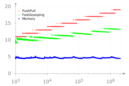
Figure 1: Comparison of the communication overhead of the gossiping methods. The $x$-axis shows the graph size, the $y$-axis the average number of messages sent per node.

Figure 2: Relative number of additional node failures in the memory model with a graph size of 1,000,000. The $x$-axis shows the number of nodes marked failed $F$, the $y$-axis the ratio of additional uninformed nodes to $F$.

Figure 1 shows an increasing gap between the message complexity of Algorithm 1 and the simple push-pull approach. Furthermore, the data shows that the number of messages sent per node in Algorithm 2 is bounded by $5$. According to the descriptions of the algorithms, each phase runs for a certain number of steps. The parameters were tuned as described in Table 1 to obtain meaningful results.

Phase	Limit	Value
Algorithm 1
I	number of steps	$\lceil 1.2\cdot\log\log{n}\rceil$
II	number of rounds	$\lceil\log{n}/\log\log{n}\rceil$
II	random walk probability	$1.0/\log{n}$
II	number of random walk steps	$\lceil\log{n}/\log\log{n}+2\rceil$
II	number of broadcast steps	$\lceil 0.5\cdot\log\log{n}\rceil$
Algorithm 2
I	first loop, number of steps (rounded to a multiple of $4$)	$2.0\cdot\log{n}$
I	second loop, number of steps	$\lfloor 2.0\cdot\log\log{n}\rfloor$
II	number of steps	corresponds to Phase I
III	number of push steps	$\lfloor\log{n}\rfloor$

Table 1: The actual constants used in our simulation.

The fact that the number of steps is a discrete value also explains the discontinuities that can be observed in the plot. In the case of the simple push-pull-approach, these jumps clearly happen whenever an additional step is required to finish the procedure. Note, that since in this approach each node communicates in every round, the number of messages per node corresponds to the number of rounds.

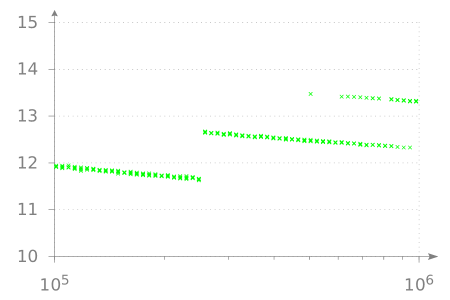
Figure 4: A more detailed view of the data presented in Figure 1 for Algorithm 1. The $x$-axis shows the graph size, the $y$-axis the number of messages sent per node.

In the case of Algorithm 1, we do not only observe these jumps, but also a reduction of the number of messages per node between the jumps. Let us consider such a set of test runs between two jumps. Within such an interval, the number of random walk steps as well as broadcasting steps remain the same while $n$ increases. The number of random walks, however, is not fixed. Since each node starts a random walk with a probability of $1/\log{n}$, the relative number of random walks decreases and thus also the average number of messages per node (see also Figure 4 in Appendix C). This shows the impact of the random walk phase on the message complexity.

The last phase of each algorithm was run until the entire graph was informed, even though the nodes do not have this type of global knowledge. From our data we observe that the resulting number of steps is concentrated (i.e., for the same $n$ the number of steps to complete only differs by at most $1$ throughout all the simulations). Furthermore, no jumps of size 2 are observed in the plot. Thus, overestimating the obtained running time by $1$ step would have been sufficient to complete gossiping in all of our test runs.

To gain empirical insights into the behavior of the memory-based approach described in Section 4 under the assumption of node failures, we implemented nodes that are marked as failed. These nodes simply do not store any incoming message and refuse to transmit messages to other nodes.

The plot in Figure 2 shows the results of simulations on an Erdős-Rényi random graph consisting of 1,000,000 nodes with an expected node degree of $\log^{2}{n}\approx 400$. Our simulation of Algorithm 2 constructed $3$ message distribution trees, independently. Afterwards we marked $F$ nodes chosen uniformly at random as failed. The nodes were deactivated before Phase II. The $x$-axis in Figure 2 shows this number of nodes $F$. In the simulation, we determined the number of initial messages that have been lost in addition to the messages of the $F$ marked nodes. Figure 2 shows on the $y$-axis the ratio of the lost messages of healthy nodes over $F$. That is, zero indicates that no additional initial message was lost, whereas 2.0 indicates that for every failed node the initial messages of at least two additional healthy nodes were not present in any tree root after Phase II.

Further plots showing additional graph sizes and various levels of detail can be found in Appendix C.

Appendix A Additional Lemmas from [19]

For some $u,v$ let $A_{u,v}$ denote the event that $u$ and $v$ are connected by an edge, and let $A_{u,v,l}$ denote the event that $u$ and $v$ share an edge and $u$ chooses $v$ in step $l$ (according to the random phone call model). In the next lemma, we deal with the distribution of the neighbors of a node $u$ in a graph $G(n,p)$, after it has chosen $t$ neighbors, uniformly at random, in $t=O(\log n)$ consecutive steps. In particular, we show that the probability of $u$ being connected with some node $v$, not chosen within these $t$ steps, is not substantially modified after $O(\log n)$ steps.

Lemmax 1 (1 of [19]).

Let $V=\{v_{1},\dots,v_{n}\}$ be a set of $n$ nodes and let every pair of nodes $v_{i},v_{j}$ be connected with probability $p$, independently, where $p\geq\log^{\delta}n/n$ for some constant $\delta>2$. If $t=O(\log n)$, $u,v\in V$, and

$$A(U_{0},U_{1},U_{2})=\bigwedge\limits_{{0<l\leq t}\atop{(v_{i},v_{j},l)\in U_{0}}}A_{v_{i},v_{j},l}\bigwedge\limits_{(v_{i^{\prime}},v_{j^{\prime}})\in U_{1}}A_{v_{i^{\prime}},v_{j^{\prime}}}\bigwedge\limits_{(v_{i^{\prime\prime}},v_{j^{\prime\prime}})\in U_{2}}\overline{A_{(v_{i^{\prime\prime}},v_{j^{\prime\prime}})}}\enspace,$$

for some $U_{0}\subset V\times V\times\{0,\dots,t\}$ and $U_{1},U_{2}\subset V\times V$, then it holds that

$$\Pr\left[(u,v)\in E\leavevmode\nobreak\ \left|\leavevmode\nobreak\ A(U_{0},U_{1},U_{2})\right.\right]=p(1\pm O(t/d)),$$

for any $U_{0},U_{1},U_{2}$ satisfying the following properties:

• $|U_{0}\cap\{(v_{i},v_{j},l)|v_{j}\in V\}|=1$ for any $v_{i}\in V$ and $l\in\{0,\dots,t\}$,

• $|U_{1}\cap\{(u,u^{\prime})|u^{\prime}\in V\}|=\Omega(d)$ and $|U_{1}\cap\{(v,v^{\prime})|v^{\prime}\in V\}|=\Omega(d)$,

• $(u,v)\not\in U_{1}\cup U_{2}$, and $(u,v,i)\not\in U_{0}$ for any $i$.

Appendix B Additional Lemmas from [20]

Lemmax 2 (2.2 from [20], adapted version).

Let Algorithm 2 be executed on the graph $G(n,p)$ of size $n$, where $p>\log^{2+\Omega(2)}n/n$ and $\rho$ is a properly chosen (large) constant. If $t=\log n+\frac{\rho}{2}\log\log n$, then $|H(t)|\leq n/\sqrt[4]{d}$ and the number of transmissions after $t$ time steps is bounded by $O(n\log\log n)$. Additionally, if $t=\log n+\frac{3\rho}{8}\log\log n$, we have $|H(t)|\geq n/\sqrt[4]{d}$.

Lemmax 3 (2.7 from [20], adapted version).

Let $|H(t)|\in[\log^{q}n,n/\sqrt[4]{d}]$ be the number of uninformed nodes in $G(n,p)$ at some time $t=O(\log n)$, where $q$ is a large constant, and let Algorithm 2 be executed on this graph. Then, $|H(t+3\rho\log\log n/8)|\leq\log^{q}n$, w.h.p., provided that $\rho$ is large enough.

Lemmax 4 (2.8 from [20], adapted version).

Let $|H(t)|\leq\log^{q}n$ be the number of uninformed nodes in $G(n,p)$ at time $t=O(\log n)$, and let Algorithm 2 be executed on this graph. Then within additional $\rho\log\log n/8$ steps all nodes in the graph will be informed, w.h.p., whenever $\rho$ is large enough.

Appendix C Further Plots and Empirical Data

C.1 Push-Pull-Algorithm

The algorithm labeled push-pull in Figure 1 is a simple procedure, where in each step every node opens a connection, performs pushpull, and closes the connection. For the sake of completeness of this paper it is described in pseudocode in Algorithm 4.

for $t=1$ to $\operatorname{O}\left(\log{n}\right)$ do

       at each node $v$ do in parallel

             pushpull($m_{v}$)

            

      

Algorithm 4 A simple push-pull algorithm to perform randomized gossiping. The pushpull operation is preceeded and followed by opening and closing a channel, respectively.

C.2 Robustness Analysis

The following plots shown in Figure 3 were run on graphs of size 100,000 and 500,000 nodes, respectively. They visualize the results of the same type of simulation as presented in Figure 2.

More detail can be obtained from the plots shown in Figure 5, where we ran our simulation with a higher resolution. That is, we ran a series of at least $5$ tests per number of failed nodes. The number of failed nodes was chosen from the set $\{0,100,200,300,\dots\}$. We used graphs of two different sizes in these 6 plots. The left column shows the results for a graph consisting of 100,000 nodes and the right column for 500,000 nodes. The $x$-axis shows the number of failed nodes, the $y$-axis shows the percentage of runs in which more than a certain number $T$ of additional nodes failed. This number is $T=0$ for the top row, $T=10$ for the middle row and $T=100$ for the bottom row. For example, this tells us that on a graph of size 100,000 more than 4000 nodes could fail and still the number of additional uninformed nodes was less than 100 in all test runs.

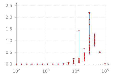
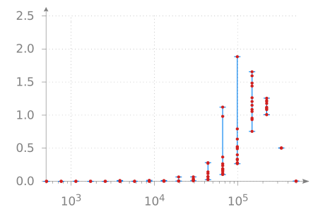
Figure 3: Relative number of additional node failures in the memory model with graphs of sizes 100,000 (top) and 500,000 (bottom). The $x$-axis shows the number of failed nodes $F$, the $y$-axis the ratio of additional uninformed nodes to $F$.

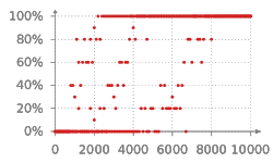
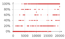
Figure 5: Detailed plot showing the robustness of Algorithm 2 on graphs of sizes 100,000 (left column) and 500,000 (right column). The $x$-axis shows the number of failed nodes, the $y$-axis shows the percentage of runs in which more than $T$ additional numbers remained uninformed. In the top $T=0$, in the middle $T=10$ and in the bottom $T=100$.

References

- [1] W. Aiello, F. Chung, and L. Lu. A random graph model for power law graphs. Experimental Mathematics, 10(1):53–66, 2001.
- [2] D. Alistarh, S. Gilbert, R. Guerraoui, and M. Zadimoghaddam. How efficient can gossip be? (on the cost of resilient information exchange). In Proc. ICALP’10, pages 115–126. 2010.
- [3] L. Becchetti, A. Clementi, E. Natale, F. Pasquale, and R. Silvestri. Plurality consensus in the gossip model. In Proc. SODA’15, to appear, 2015.
- [4] E. A. Bender and E. Canfield. The asymptotic number of labeled graphs with given degree sequences. J. of Combinatorial Theory, Series A, 24(3):296–307, 1978.
- [5] P. Berenbrink, J. Czyzowicz, R. Elsässer, and L. Gąsieniec. Efficient information exchange in the random phone-call model. In Proc. ICALP’10, volume 6199. 2010.
- [6] P. Berenbrink, R. Elsässer, and T. Friedetzky. Efficient randomised broadcasting in random regular networks with applications in peer-to-peer systems. In Proc. PODC’08, pages 155–164, 2008.
- [7] P. Berenbrink, R. Elsässer, and T. Sauerwald. Communication complexity of quasirandom rumor spreading. Algorithmica, pages 1–26, 2014.
- [8] D. Bertsekas and J. Tsitsiklis. Parallel and Distributed Computation – Numerical Methods. Prentice Hall, 1989.
- [9] B. Bollobás. A probabilistic proof of an asymptotic formula for the number of labelled regular graphs. European J. of Combinatorics, 1(4):311–316, 1980.
- [10] B. Bollobás. Random Graphs. Cambridge University Press, 2nd edition, 2001.
- [11] S. Botros and S. Waterhouse. Search in JXTA and other distributed networks. In P2P’01, pages 30–35, 2001.
- [12] K. Censor-Hillel and H. Shachnai. Fast information spreading in graphs with large weak conductance. SIAM J. on Computing, 41(6):1451–1465, 2012.
- [13] J. Chen and G. Pandurangan. Almost-optimal gossip-based aggregate computation. SIAM J. on Computing, 41(3):455–483, 2012.
- [14] F. Chierichetti, S. Lattanzi, and A. Panconesi. Rumour spreading and graph conductance. In Proc. SODA’10, pages 1657–1663, 2010.
- [15] C. Cooper, A. Frieze, and T. Radzik. Multiple random walks in random regular graphs. SIAM J. Discrete Math., 23(4):1738–1761, 2009.
- [16] A. Demers, D. Greene, C. Hauser, W. Irish, J. Larson, S. Shenker, H. Sturgis, D. Swinehart, and D. Terry. Epidemic algorithms for replicated database maintenance. In Proc. PODC’87, pages 1–12, 1987.
- [17] B. Doerr, M. Fouz, and T. Friedrich. Social networks spread rumors in sublogarithmic time. In Proc. STOC’11, pages 21–30, 2011.
- [18] B. Doerr, T. Friedrich, and T. Sauerwald. Quasirandom rumor spreading: Expanders, push vs. pull, and robustness. In Proc. ICALP’09, pages 366–377, 2009.
- [19] R. Elsässer. On the communication complexity of randomized broadcasting in random-like graphs. In Proc. SPAA’06, pages 148–157, 2006.
- [20] R. Elsässer and T. Sauerwald. The power of memory in randomized broadcasting. In Proc. SODA’08, pages 218–227, 2008.
- [21] R. Elsässer and T. Sauerwald. Cover time and broadcast time. In Proc. STACS’09, pages 373–384, 2009.
- [22] P. Erdős and A. Rényi. On random graphs. Publ. Mathematicae Debrecen, 6:290–297, 1959.
- [23] U. Feige, D. Peleg, P. Raghavan, and E. Upfal. Randomized broadcast in networks. Random Structures & Algorithms, 1(4):447–460, 1990.
- [24] N. Fountoulakis, A. Huber, and K. Panagiotou. Reliable broadcasting in random networks and the effect of density. In Proc. INFOCOM’10, pages 1–9, 2010.
- [25] P. Fraigniaud and E. Lazard. Methods and problems of communication in usual networks. Discrete Applied Mathematics, 53(1–3):79 – 133, 1994.
- [26] G. Giakkoupis. Tight bounds for rumor spreading in graphs of a given conductance. In Proc. STACS’11, pages 57–68, 2011.
- [27] G. Giakkoupis. Tight bounds for rumor spreading with vertex expansion. In Proc. SODA’14, pages 801–815, 2014.
- [28] G. Giakkoupis and T. Sauerwald. Rumor spreading and vertex expansion. In Proc. SODA’12, pages 1623–1641, 2012.
- [29] Gnutella. The annotated Gnutella protocol specification v0.4.
- [30] B. Haeupler. Tighter worst-case bounds on algebraic gossip. IEEE Communications Letters, 16(8):1274–1276, 2012.
- [31] B. Haeupler. Simple, fast and deterministic gossip and rumor spreading. In Proc. SODA’13, pages 705–716, 2013.
- [32] T. Hagerup and C. Rüb. A guided tour of chernoff bounds. Information Processing Letters, 33(6):305–308, 1990.
- [33] J. Hromkovič, R. Klasing, A. Pelc, P. Ruzicka, and W. Unger. Dissemination of Information in Communication Networks. Springer, 2005.
- [34] R. Karp, C. Schindelhauer, S. Shenker, and B. Vocking. Randomized rumor spreading. In Proc. FOCS’00, pages 565–574, 2000.
- [35] D. Kempe, A. Dobra, and J. Gehrke. Gossip-based computation of aggregate information. In Proc. FOCS’03, pages 482–491, 2003.
- [36] A.-M. Kermarrec, L. Massoulie, and A. Ganesh. Probabilistic reliable dissemination in large-scale systems. Parallel and Distributed Systems, IEEE Transactions on, 14(3):248–258, 2003.
- [37] D. Mosk-Aoyama and D. Shah. Computing separable functions via gossip. In Proc. PODC ’06, pages 113–122, 2006.
- [38] R. Motwani and P. Raghavan. Randomized Algorithms. Cambridge University Press, 1995.
- [39] B. Pittel. Linear probing: The probable largest search time grows logarithmically with the number of records. J. of Algorithms, 8(2):236–249, 1987.
- [40] M. Raab and A. Steger. Balls into bins – a simple and tight analysis. In Proc. RANDOM’98, pages 159–170. 1998.
- [41] N. C. Wormald. The asymptotic connectivity of labelled regular graphs. J. of Combinatorial Theory, Series B, 31(2):156–167, 1981.
- [42] N. C. Wormald. The asymptotic distribution of short cycles in random regular graphs. J. of Combinatorial Theory, Series B, 31(2):168–182, 1981.
- [43] N. C. Wormald. Models of Random Regular Graphs. In Surveys in Combinatorics, 1999, volume 267 of London Mathematical Society Lecture Note Series, pages 239–298. Cambridge University Press, 1999.