Extensive numerical investigations on the ergodic properties
of two coupled Pomeau-Manneville maps

Abstract

We present extensive numerical investigations on the ergodic properties of two identical Pomeau-Manneville maps interacting on the unit square through a diffusive linear coupling. The system exhibits anomalous statistics, as expected, but with strong deviations from the single intermittent map: Such differences are characterized by numerical experiments with densities which do not have singularities in the marginal fixed point, escape and Poincaré recurrence time statistics that share a power-law decay exponent modified by a clear dimensional scaling, while the rate of phase-space filling and the convergence of ensembles of Lyapunov exponents show a stretched instead of pure exponential behaviour. In spite of the lack of rigorous results about this system, the dependence on both the intermittency and the coupling parameters appears to be smooth, paving the way for further analytical development. We remark that dynamical exponents appear to be independent of the (nonzero) coupling strength.

1 Introduction

Intermittent systems represent a paradigmatic example of weak chaos, where chaotic domains coexists with regular, non-chaotic structures. Typical examples of such a situation involve area preserving maps (see for example [1, 2, 3]), where regular structures often occupy a finite fraction of the whole phase-space. On the other side, intermittent systems having a zero-measure source of non-hyperbolicity or regular motion often allow more quantitative considerations, a typical example being Pomeau-Manneville (PM) maps [4], for which many peculiar properties (from power-law correlation decay to generalised central limit theorems to infinite ergodic theory), have been anticipated by Gaspard and Wang [5, 6] and later discussed and proved in several papers, with also remarkable applications to the problem of anomalous transport.

In this work we address the important problem of multidimensional extension of such prototypical models by diffusively coupling [7, 8] a pair of Pomeau-Manneville maps: it is not trivial, indeed, how the increased dimensionality may modify the dynamical properties, e.g. allowing the system to avoid or deform the intermittent behaviour. In other words, we are interested in characterising the ergodic properties of two coupled PM maps and compare this case with the single PM map results. Among the different tools to investigate such properties a prominent role is played by the analysis of phase-space densities, escape and recurrence time statistics, filling rates and finite-time Lyapunov statistics. Apart from the intrinsic interest, this study represents a natural preliminary step towards many-dimensional extensions, which have been recently proposed, for example, as the proper framework to study the statistics of genomic sequences [9].

The paper is organised as follows: Section 2 describes general properties of the 1D PM map and its 2D version (PM2) coupled via the diffusive scheme; stability arguments allow to identify and avoid the so-called synchronization regime. In Section 3 we present and discuss the numerical results that are summarised in the conclusions in Section 4.

2 General setting

2.1 Pomeau-Manneville (PM) map

The PM map is a non-invertible transformation of the unit-interval $f_{z}:[0,1]\circlearrowleft$, defined by:

$$x\ \mapsto\ f_{z}(x)\ =\ x\,+\,x^{z}\mod 1$$

$$=\ x\,+\,x^{z}\,-\,\chi_{z}(x),$$ (1)

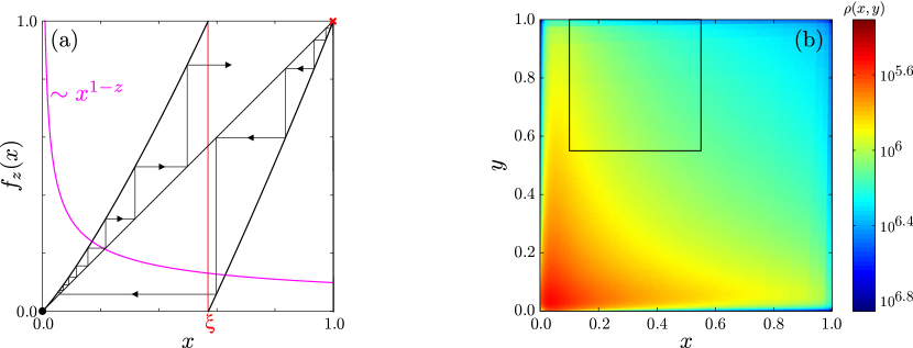
where $1<z\in\mathbb{R}$ and $\chi_{z}(x)$ is the characteristic function of the set $[\xi,1]$ (i.e. $\chi_{z}(x)=0$ for $x<\xi$, and $\chi_{z}(x)=1$ for $x\geq\xi$) with the discontinuity point $\xi(z)<1$ defined by $f_{z}(\xi)=1$. As we remarked in the introduction, we are interested in the regime where the fixed point at $0$ is not hyperbolic: this happens whenever $z>1$; notice that when $z=1$ (1) yields the -fully chaotic- Bernoulli map). Thus, for $z>1$, at the fixed point at the origin we have $f^{\prime}(0)=1$, namely we have an indifferent fixed point, neither stable nor unstable, as far as linear analysis is concerned. The dynamical properties of the PM map are determined by its indifferent fixed point at $x=0$, where the dynamics is slowed down by the tangency (see Fig. 1(a)), and they strongly depend on the intermittency parameter $z$. When $z>2$ there is no invariant probability measure (the invariant density close to the origin goes as $x^{1-z}$) and the map (1) provides and example of infinite ergodicity [10, 11, 12]: We will not consider such a case in the present paper. On the other hand, we are interested in the regime $1<z<2$ where the map is ergodic and the invariant measure close to the origin has the same behaviour as before, but now with an integrable singularity [13]. For such intermittency parameter range the map is also mixing, with polynomial decay of correlation functions: the corresponding power-law exponent $\Gamma$ (such that, asymptotically, the mixing speed is $n^{-\Gamma}$) can be expressed in terms of the intermittency parameter as follows [6, 14]:

$$\Gamma=\frac{1}{z-1}-1.$$ (2)

Notice that, when $z\geq 3/2$, correlations are not integrable i.e. $\int\,dt\,C(t)$ diverges: a striking dynamical manifestation of this observation is that a generalized central limit theorem holds with properly scaled sums converging to a Lévy stable law [15].

2.2 Coupling scheme

We start our analysis by considering two identical copies of the PM map $f_{z}$ given by Eq. (1) interacting on the unit square $S=[0,1]^{2}$ through the application of a linear diffusive coupling; this leads to the following 2D (PM2) map:

$$\mathbf{f}_{z,\varepsilon}:\ \left[\begin{array}[]{c}x\\ y\end{array}\right]\ \mapsto\ \left[\begin{array}[]{c}f_{z}\left(\,x\,+\,\varepsilon\left(y-x\right)\,\right)\\ f_{z}\left(\,y\,-\,\varepsilon\left(y-x\right)\,\right)\end{array}\right]\ ;$$ (7)

which corresponds to the map considered in Ref. [7] with the nonlinear and coupling parts applied in reverse order. This choice allows to define Poincaré recurrences in a proper way: indeed, the coupling part maps the unit square $S$ into a smaller sub-set contained in S (see Fig. 1 in Ref. [7]) which then becomes the actual phase-space for the map. Instead, by applying the nonlinear part after the coupling, as in Eq. (7), we ensure that the mapping is onto $S$. The linear coupling in Eq. (7) is the two-maps limit of the renown Laplacian or diffusive coupling for a chain of $N$ coupled maps $\{x_{j}\}_{j=1..N}$ with periodic boundary conditions $x_{N+1}=x_{1}$ [8]. The choice of this coupling is motivated by its simplicity, being linear, and by the fact that it converges to the Laplace operator in the limit $N\to\infty$ of a continuous closed chain of maps.

Figure 1: (Color online) Panel (a): Phase-space dynamics of the PM map, given by Eq. (1), with $z=1.5$ and $\xi(z)\simeq 0.57$, along with a typical orbit: after being quickly repelled away from the unstable fixed point at $x=1$ (red cross) and being re-injected into $[0,\xi]$, it slowly escapes from the indifferent fixed point at $x=0$ (black point). The nearer the reinjection is to $x=0$, the longer the escape lasts, leading to an invariant density with a singularity $\sim x^{1-z}$ at $x=0$ (magenta-continuous line). Panel (b): in color, the two-dimensional numerical density of points $\rho(x,y)$ (the color-bar is presented in logarithmic scale) for an orbit of length $10^{11}$ of the coupled PM2 map (see Eq. 7) with $z=1.5$ and $\varepsilon=10^{-2}$; the orbit visits the whole partition of $10^{3}\times 10^{3}$ cells, but the color levels reveal that the density is not the product of two PM densities. The upper left square is the region over which recurrences are computed (Sec. 3.4); this is chosen to avoid the synchronized states on the diagonal.

2.2.1 Linear stability

In the case of two coupled maps, the diagonal $x=y$ of the unit square is an invariant set for map (7) (we may call it the set of synchronized states of the system); it is thus informative to study its stability properties. For points $\mathbf{x}=(x,x)$, the first/second eigenvector of the Jacobian matrix of map (7) is respectively parallel/orthogonal to the diagonal itself; a calculation analogous to Ref. [7] allows to compute the two Lyapunov exponents of the diagonal:

$$\lambda_{1}^{diag}=\lambda^{1\textnormal{D}},\quad\lambda_{2}^{diag}=\lambda^{1\textnormal{D}}+\ln(1-2\varepsilon)<\lambda_{1};$$ (8)

with $\lambda^{1\textnormal{D}}$ the Lyapunov exponent of the 1D Pomeau-Manneville map (1) with initial condition $x$; from the expression for the second exponent $\lambda_{2}^{diag}$ one can see that, when the coupling parameter $\varepsilon$ is large enough, $\lambda_{2}^{diag}$ becomes negative and the diagonal turns into an attracting set, leading to global synchronization [16, 17] (that is, the system synchronizes for any initial condition in the unit square $S$). Thus, by setting $\lambda_{2}^{diag}=0$, the critical coupling value $\varepsilon_{cr}$ above which synchronization appears is obtained:

$$\varepsilon_{cr}=\frac{1-e^{-\lambda^{1\textnormal{D}}}}{2},$$ (9)

and it depends on parameter $z$ trough the exponent $\lambda^{1\textnormal{D}}$; this relation holds for any pair of diffusively coupled, identical 1D maps. In the following we will only consider the range $\varepsilon\ll\varepsilon_{cr}$, i.e., avoiding synchronization; this is achieved by a preliminary estimate of the 1D Lyapunov exponent $\lambda^{1\textnormal{D}}$ for the chosen value of $z$. Notice that, in the range $z\in]1,2[$ we consider here, the Lyapunov exponent $\lambda^{1\textnormal{D}}$ is always positive for any initial condition $\mathbf{x}=(x,x)\neq(0,0)$; instead, the exponent $\lambda^{1\textnormal{D}}$ vanishes for the fixed point in the origin $(0,0)$, so the two Lyapunov exponents for such point read:

$$\lambda_{1}^{(0,0)}=0,\quad\lambda_{2}^{(0,0)}=\ln(1-2\varepsilon)<0.$$ (10)

This implies that the stability of fixed point $(0,0)$ is discontinuous in $\varepsilon=0$ : for $\varepsilon>0$ it is marginal along the diagonal ($\lambda_{1}^{(0,0)}=0$) and contracting along the anti-diagonal ($\lambda_{2}^{(0,0)}<0$), while for $\varepsilon=0$ it is marginal along both the eigenvectors, since $\lambda_{2}^{(0,0)}\to\lambda_{1}^{(0,0)}=0$ smoothly as $\varepsilon\to 0$. Interestingly, this scenario holds even in the non-synchronizing regime, when the diagonal is repelling ($\lambda_{2}^{diag}>0$). This is a first hint about the structural change in the map caused by the coupling: in the uncoupled case $\varepsilon=0$, the whole neighbourhood of the origin is affected by its marginal stability and the associated slow-down; instead, in the coupled case $\varepsilon\neq 0$ the slow-down affects only the diagonal, while the infinitesimal neighbourhood of the origin is contracted toward the diagonal along its transversal direction. This is confirmed by the numerical phase-space densities presented in the next Section.

3 Numerical results

3.1 Ergodicity test 1: Phase-space densities

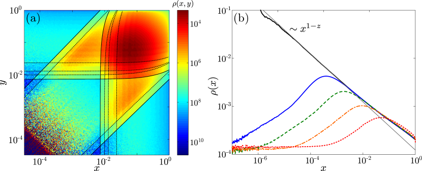
To analyse the phase-space structure of the PM2 map, we compute numerical densities for orbits of length $10^{9}$ over a square grid of $10^{3}\times 10^{3}$ cells (Fig. 1(b)): this shows that no dynamical barriers are present, with the orbit visiting all the cells of the partition even for arbitrarily small couplings. The observation of inhomogeneities in a small neighbourhood of the origin leads us to perform the same phase-space analysis employing a square-grid partition in logarithmic scale for coordinates $x$ and $y$, as presented in the Fig. 2(a): this reveals that the density is dominated by a very complicated structure of discontinuity lines which delimit regions with much higher density. The reading of such logarithmic color-map should be compared with its corresponding linear version in Fig. 1(b), to conclude that the observed orbit tends to avoid the coordinate axes while visiting much more frequently the central maximum away from the origin. Such behaviour is in clear opposition to the classic divergence of the PM density in the origin (see also Fig. 1(a)) and is reflected in the marginal distributions for the single coordinate $x$ for the PM2 map (Fig. 2(b)): a comparison with the corresponding distribution for a PM orbit with the same intermittency parameter shows that, while the 1D distribution diverges in the origin as $\sim x^{1-z}$, the 2D distributions for all $\varepsilon\neq 0$ have a maximum away from the origin; this appears to move continuously toward $x=0$ as $\varepsilon\to 0$. This phenomenon is robust against different sizes of phase-space partition, proving that the effect of arbitrarily small couplings have a strong impact on both the dynamics and statistics of the system. Even more interestingly, the location of the discontinuity lines in the PM2 phase-space densities can be computed analytically: in Fig. 2(a), the solid and dashed curves are respectively the first and second iterates of the coordinate axes $x=0$ and $y=0$, while all the remaining discontinuities are checked to be higher iterates of the same sets. This unexpected phenomenon is in agreement with the estimates of the Lyapunov exponents from previous Section: the fixed point in the origin $(0,0)$ is no more completely marginal, but has one negative Lyapunov exponent which attracts the orbit toward the diagonal; at the same time, we choose parameters for which the diagonal is instead repelling. This produces the net effect of enhancing the density in a region away from the origin, differently from the uncoupled and 1D case.

Figure 2: (Color online) Panel (a): in color, the two-dimensional numerical density of points $\rho(x,y)$ (the color-bar is presented in logarithmic scale) for an orbit of length $10^{11}$ collected over a logarithmic square-grid of $10^{3}\times 10^{3}$ for the PM2 map (7) with $z=1.5$ and $\varepsilon=10^{-2}$. The black-continuous (-dashed) curves are respectively, the first (second) iterates of the axes $x=0$ and $y=0$. Over such curves and also over the higher iterates (not shown), the density appears discontinuous. Panel (b): marginal distributions $\rho(x)$ for the coordinate $x$ of the same orbit in panel (a) for $\varepsilon=0$ (black curve), $10^{-5}$ (blue curve), $10^{-4}$ (green-dashed curve), $10^{-3}$ (orange-dash-dotted curve) and $10^{-2}$ (red-dotted curve); the gray lines is the standard estimate $\sim x^{1-z}$ for the PM density.

3.2 Ergodicity test 2: Filling rate

To characterize the ergodic properties of the PM2 map we employ the filling rate method discussed in Ref. [18] for the same phase-space partition of $K=2000\times 2000$ square cells, and consider the following indicator:

$$\mathcal{Q}_{K}(n)=\frac{\textit{number of unvisited cells up to the n-th iteration}}{K}.$$ (11)

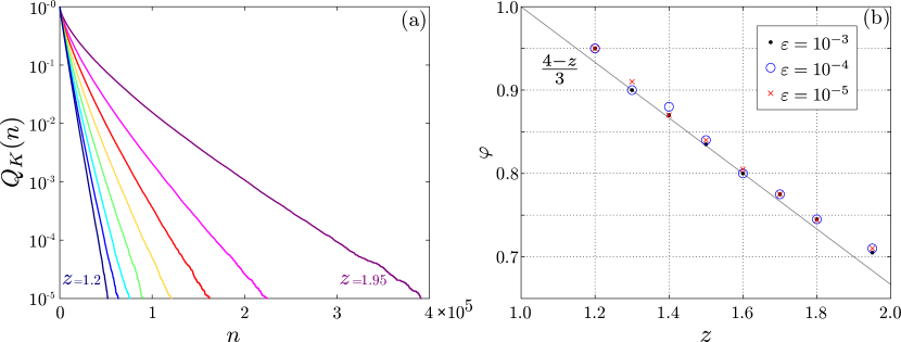
which represents the fraction of partition that is not yet visited by an orbit after $n$ iterations. A numerical verification of ergodicity is equivalent to check that function $\mathcal{Q}_{K}(n)$ vanishes in the long time limit $n\to\infty$, independently on how fine we choose the phase-space partition (i.e. in the large $K$ limit). In Fig. 3(a), a set of examples shows how indeed $\mathcal{Q}_{K}(n)$ converges to zero, confirming the observations from previous section (eventually, the orbit visits all the cells of the grid for all values of parameters $\varepsilon$ and $z$ considered here, see Fig. 3(b)). In addition to the qualitative check for ergodicity, it is informative to study also how $\mathcal{Q}_{K}(n)$ decays to zero: for models of fully chaotic dynamics, this is expected to be a pure exponential  [18] $\mathcal{Q}_{K}(n)\sim e^{-n/K}$. While generalisations of such a decay have been proposed [19], we remark that in [20] a pure exponential decay has been observed, despite the model under investigation is a billiard table shaped like a fully irrational triangle, a system with very weak ergodic properties. In our simulations we never get any evidence of such a simple asymptotics, while the data are fitted by stretched exponentials, with stretching exponent $\varphi$ and pre-factor $C$:

$$\mathcal{Q}_{K}(n)\sim e^{-C\,\cdot\,n^{\varphi}}.$$ (12)

The resulting exponents are plotted in Fig. 3(b), which suggests a linear relation with the intermittency parameter $z$ that is independent on the coupling parameter $\varepsilon$; interestingly, the latter turns out to influence only the exponent pre-factor $C$ (not shown), a property shared also by other dynamical indicators we consider in the next sections. Stretched exponential relaxations are known to have physical relevance (see for example Refs. [21, 22]): in the present context we have not any dynamical clue for this behaviour, which will be observed for other dynamical quantities in the final part of the present section.

Figure 3: (Color online) Panel (a): stretched exponential decay of $\mathcal{Q}_{K}(n)$ (fraction of unvisited cells at time $n$) for the values of intermittency exponent $z=1.2,1.3,1.4,1.5,1.6,1.7,1.8,1.95$ (respectively from left- to right-most graph) at coupling parameter $\varepsilon=10^{-4}$; the total number of cells $K=2000\times 2000$ is eventually visited, but the plot is truncated at $\mathcal{Q}_{K}(n)=10^{-5}$ for clarity. Panel (b): the stretching-exponent $\varphi$ from Eq. (12) as a function of $z$ for the three coupling parameters $\varepsilon=10^{-3},\ 10^{-4},\ 10^{-5}$; in all three cases the almost linear trends are close to the line $(4-z)/3$ (in grey, for reference), leading to pure exponential at $z=1$ (i.e. the Bernoulli map limit).

3.3 A warm up exercise: Escape from the indifferent region

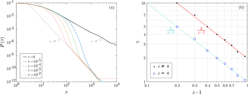
It is well known that direct numerical indications of mixing are extremely hard to attain for non trivial systems [23]: tests that proved to be numerically stabler involve either statistics of Poincaré recurrences [24, 25, 26, 27] or large deviations for Birkhoff sums [28]. As a preliminary step, we consider escape rates from a small region of the phase space containing the origin: for intermittent dynamics we expect a power-law decay of the surviving probability. Our numerical results refer to the choice of the escape region $\Omega=\{(x,y)\in[0,0.1]^{2}\}$, we checked that our results remain unaltered for smaller escape sets. The plots presented in Fig. 4 are obtained by choosing a uniformly distributed ensemble of $10^{10}$ initial conditions in $\Omega$, and computing the cumulative survival probability $P_{\Omega}(\tau)$. For uncoupled ($\varepsilon=0$) maps, since the set of points that survive $n$ iterations is a square, whose construction is easily induced by the 1D case [6], we expect that $P_{\Omega}(\tau)\sim\tau^{-\gamma^{\varepsilon=0}_{esc}}$ where the exponent is twice the value for 1D PM maps, $\gamma^{\varepsilon=0}_{esc}=2/(z-1)$. From Fig. 4 we observe that the escape power laws follow very closely the uncoupled behaviour over a wide set of coupling constants $\varepsilon$. This result is however only a probe of local properties close to the indifferent fixed point, so we now turn to more meaningful tests of mixing properties.

Figure 4: (Color online) Cumulative probability distributions of escape times for 2 coupled PM maps with $z=1.2,1.3,1.4,1.5,1.6,1.7,1.8,1.95$ and $\varepsilon=10^{-2}$ (red-continuous curves), $\varepsilon=10^{-3}$ (yellow-continuous curves), $\varepsilon=10^{-4}$ (green-continuous curves), $\varepsilon=10^{-5}$ (blue-continuous curves) and $\varepsilon=0$ (black-continuous curves); the escape is computed from the hyper-cube with side $0.1$ located in the corner of the origin. All numerical data agree very well with the estimate $\gamma_{esc}=2/(z-1)$ represented by dashed-black curves.

3.4 Mixing test 1: Recurrence times

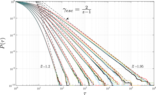
In this Subsection we present numerical experiments for the statistics of Poincaré recurrences in a fixed box in phase space: we choose $(x,y)\in[0.10,0.55]\times[0.55,1.00]={\cal X}\times{\cal Y}$ away from the diagonal (synchronized states), and a single random initial condition was iterated until the ensemble of recurrences was equal to $10^{12}$. We also tested boxes with different sizes and the quantitative results remain unaltered. We remark that such a huge ensemble of recurrences is essential to get a reliable statistics for long return times. To visualize the data we plot the cumulative probability $P_{rec}(\tau)\ \mathrel{\mathop{:}}=\ P(t_{rec}\geq\tau)$ for the orbit to return in the box only after a certain time $\tau$: if the cumulative probability decays polynomially with an exponent $\gamma$, then we expect [24, 25, 26] that also correlations display a power-law decay, with an exponent $\Gamma=\gamma-1$. By such analysis, in Fig. 5(a) we confirm the presence of an asymptotic power-law decay:

$$P_{rec}(\tau)\sim\tau^{-\gamma}$$ (13)

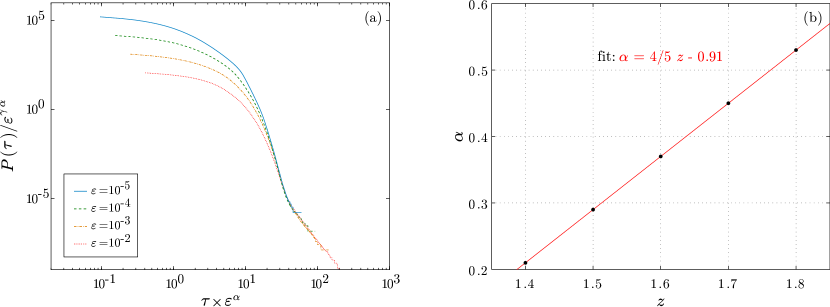
whose exponent $\gamma$ depends on the intermittency parameter $z$ but not on the diffusive coupling $\varepsilon$. As illustrated in Fig. 5(b), such dependence for $\varepsilon>0$ coincides with twice the exponent behaviour for the case $\varepsilon=0$ , that is $\gamma(z)\sim 1/(z-1)$, namely the exponent of the 1D map (see Ref. [29] for an early derivation of such a formula, based on escape rates from the indifferent fixed point). We may understand the $\varepsilon=0$ behaviour by a qualitative argument as follows: if we consider return times on a strip $(x,y)\in{\cal X}\times[0,1]$ then the statistics is determined by the single PM map for the variable $x$, and so Poincaré recurrences $n_{1},\,n_{2}\,\cdots n_{k}\cdots$ are ruled by the exponent of the 1D map. If we now slice the strip into $M$ pieces, one being ${\cal X}\times{\cal Y}$, returns are now $\tilde{n}_{1},\,\tilde{n}_{2},\cdots\tilde{n}_{j}\cdots$, where $\tilde{n}_{m}=\sum_{s}\,n_{s}$ for some set, until the box is hit again. Since we are away from the intermittent region we may expect that arrival probabilities in the $M$ cells are essentially uniform, so, while the $\tilde{n}_{l}$ sequence has roughly a mean value which is $M$ times that of the $n_{j}$ sequence, we expect the tail of the distribution to be governed by the same power law. Our numerical results suggest, once again, that, at least asymptotically, any non-zero coupling induces instead uncorrelated behaviour on the two maps return probabilities. Nevertheless the deviation from the uncoupled distribution (thick-solid curve in Fig. 5(a)) takes place at longer return-times as the coupling parameter $\varepsilon$ is reduced (thin-curves in Fig. 5(a)). The coupling parameter $\varepsilon$ influences only the pre-asymptotic decay, suggesting the existence of a scaling law: indeed observing Fig. 6(a) we find it by writing $P(\tau)$ in the following form:

$$P_{rec}(\tau)\ \sim\ \varepsilon^{\gamma\alpha}\mathcal{F}(\tau\varepsilon^{\alpha}),$$ (14)

where $\gamma$ is the power-law decay exponent, $\alpha$ is a fitting parameter and $\mathcal{F}$ is a function independent on $\varepsilon$. An appropriate choice of $\alpha$ allows to get curve collapsing in the asymptotic power-law regime. We remark again that up to some $\varepsilon$ depending transient time the dynamics is instead dominated by the uncoupled behavior. In Fig. 6(b), the plot of $\alpha$ as a function of the intermittency parameter $z$ shows a behaviour that is quite accurately reproduced by a linear fit with slope $\sim 4/5$.

Figure 5: (Color online) Panel (a): Cumulative probability for recurrence times $\tau$ at $z=1.5$ and coupling parameter $\varepsilon=10^{-2},10^{-3},10^{-4},10^{-5},0$; dashed and dash-dotted lines are fits to the power-law decay of respectively the uncoupled ($\varepsilon=0$) and coupled ($\varepsilon>0$) cases. Panel (b): The same power-law exponents for the set of intermittency exponents under study $z=1.2,1.3,1.4,1.5,1.6,1.7,1.8,1.95$; we find the same exponents for all $\varepsilon>0$ cases (black points, red-continuous line $\sim 2/(z-1)$ for reference), and all of them coincide with twice the $\varepsilon=0$ exponents (blue circles, light-blue-dashed line $\sim 1/(z-1)$ for reference). Notice that the characteristic time at which the power-law starts grows as the coupling parameter $\varepsilon\to 0$.

Figure 6: (Color online) Panel (a): Cumulative probability of recurrence times $\tau$ at $z=1.5$ (same as in Fig. 5(a)) after rescaling according to Eq. (14). Panel (b): The rescaling exponent $\alpha$ as a function of parameter $z$, for the cases in which the curve collapse is apparent; the solid-red line is a linear fit.

3.5 Mixing test 2: Finite time Lyapunov exponents

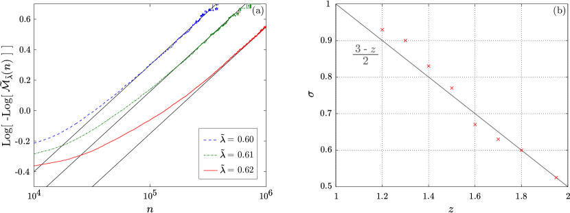
An alternative indirect way of probing mixing speed is provided by large deviation analysis of the largest finite-time Lyapunov exponents: this method is based upon rigorous results, proved in Refs. [30, 31] (see also [32]), and it was numerically tested on intermittent and Hamiltonian systems in Ref. [28]. Since it is a less widely used technique with respect to scrutinizing the statistics of Poincaré recurrences, we briefly recall how it works operationally: for further details see Ref. [28]. The crucial quantity to take into account is the probability distribution of finite-time Lyapunov exponents $\mathcal{P}_{n}(\lambda)$ (leading expansion rates up to some fixed time $n$) which, for an ergodic system, collapses to a Dirac delta in the $n\to\infty$ limit. The idea [30, 31, 32] is that, by fixing a threshold $\tilde{\lambda}<\lambda_{\infty}$ ($\lambda_{\infty}$ being the asymptotic largest Lyapunov exponent) one can define:

$$\mathcal{M}_{\tilde{\lambda}}(n)=\int_{0}^{\tilde{\lambda}}\,d\lambda\,\mathcal{P}_{n}(\lambda),$$ (15)

such that (in a large deviation philosophy) the way $\mathcal{M}_{\tilde{\lambda}}(n)$ decays as $n\to\infty$ should also rule the mixing speed. We underline that the important issue is that intermittent dynamics deeply modifies large deviations properties: the measure of point where Birkhoff sums up to time $n$ are at least $\epsilon$ different from the asymptotic average is not exponentially vanishing as $n\to\infty$, but decays with a weaker power law, whose exponent coincide with the one ruling correlations decay. The result is independent on the choice of threshold $\tilde{\lambda}$ as long as it is below the asymptotic $\lambda_{\infty}$; however, in numerical implementations one has to make preliminary checks (see Fig. 7(a)) to fix the threshold reasonably (not too close to $\lambda_{\infty}$ to spoil statistics, not too small to have only few points in the tail). The procedure we follow here (not knowing a priori the invariant measure) is to follow a single trajectory for $10^{12}$ time steps and re-construct $\mathcal{P}_{n}(\lambda)|_{n\leq 10^{6}}$ from $10^{6}$ consecutive chunks of trajectory: the threshold is then fixed depending on the goodness of the collected statistic. In Fig. 7(a) we find that, like in the case of filling rates, the data are best fitted by a stretched exponential decay $\mathcal{M}_{\tilde{\lambda}}(n)\sim e^{-C\cdot n^{\sigma}}$; notice that different values of $\tilde{\lambda}$ give the same stretching-exponent $\sigma$ but different pre-factors $C$. We find that the exponent $\sigma$, at diffusive coupling $\varepsilon=10^{-5}$, display a roughly linear dependence on parameter $z$ (Fig. 7(b)). Finally, we remark that the discrepancy between the stretched exponential for the $\mathcal{M}_{\tilde{\lambda}}(n)$ integral and the power-law decay for Poincaré recurrences definitely deserves further studies, since, in principle, the two should be related.

Figure 7: (Color online) Panel (a): Examples of stretched exponential fits for the decay of $\tilde{\mathcal{M}}_{\tilde{\lambda}}(n)\ \mathrel{\mathop{:}}=\ {\mathcal{M}}_{\tilde{\lambda}}(n)/{\mathcal{M}}_{\tilde{\lambda}}(0)$ (i.e. Eq. (15) normalized w.r.t. $n=0$ for fitting purposes) for parameters $z=1.5$, $\varepsilon=10^{-5}$ and three different values of $\tilde{\lambda}$; notice that the stretching exponent is the same for all three cases, but the exponential pre-factors are not. Panel (b): The stretching exponent $\sigma$ as a function of $z$ at $\varepsilon=10^{-5}$; the straight continuous-black line is for reference.

4 Conclusions

In summary we have mainly investigated the ergodic properties of two diffusively coupled, identical Pomeau-Manneville maps. In particular we have characterised how single trajectories fill fine partitions of the phase-space: this yields an indication of ergodicity, with a nontrivial filling rate in the form of a stretched exponential. The same time-law appears in the decay of sub-threshold finite-time Lyapunov exponent distribution, which probes the speed of mixing. By contrast, a polynomial decay is instead observed when considering the statistics of escape times and Poincaré recurrences. In addition, the latter display a power-law exponent, for two coupled maps, which is exactly twice the value for the single Pomeau-Manneville map, suggesting some kind of asymptotic independence between the two coordinates.

References

- [1] A.J. Lichtenberg and M.A. Lieberman, Regular and chaotic dynamics (Springer-Verlag, New York, 1992).
- [2] G.M. Zaslavsky, Phys. Rep. 371, 461 (2002).
- [3] C. Manchein, M.W. Beims, Phys. Lett. A 377, 789 (2013).
- [4] Y. Pomeau, P. Manneville, Commun. Math. Phys. 74, 189 (1980).
- [5] P. Gaspard, X.J. Wang, Proc. Natl. Acad. Sci. USA 85, 4591 (1988).
- [6] X.J. Wang, Phys. Rev. A 40, 6647 (1989).
- [7] A.S. Pikovsky, P. Grassberger, J. Phys. A: Math. Gen. 24, 4587 (1991).
- [8] J.-R. Chazottes and B. Fernandez, Dynamics of coupled map lattices and of related spatially extended systems, Volume 671 of Lecture Notes in Physics, (Springer-Verlag, Berlin, 2005).
- [9] A. Provata, C. Beck, Phys. Rev. E 86, 046101 (2012).
- [10] J. Aaronson, An introduction to infinite ergodic theory, (Providence, AMS, 1997).
- [11] R. Zweimüller, Ergod. Th. & Dynam. Sys. 20, 1519 (2000).
- [12] G. Bel, E. Barkai, Europhys. Lett. 74, 15 (2006).
- [13] We point out that dynamical issues might be also studied through the dense set of (unstable) periodic orbits, see for instance: R. Artuso, P. Cvitanović, G. Tanner, Progr. Theor. Phys. Suppl. 150, 1 (2003).
- [14] H. Hu, Ergod. Th. & Dynam. Sys. 24, 495 (2004).
- [15] S. Gouëzel, Th. & Rel. Fields, 128, 82 (2004).
- [16] A. Pikovsky, M. Rosenblum, J. Kurths. Synchronization: A universal concept in nonlinear sciences, (Cambridge, CUP, 2001).
- [17] S. Boccaletti, J. Kurths, G. Osipov, D.L. Valladares, C.S. Zhou, Phys. Rep. 366, 1 (2002).
- [18] M. Robnik, J. Dobnikar, A. Rapisarda, T. Prosen, M. Petrovs̆ek, J. Phys. A: Math. Gen. 30, L803 (1997).
- [19] T. Prosen, M. Robnik, J. Phys. A: Math. Gen. 31, L345 (1998).
- [20] G. Casati, T. Prosen, Phys. Rev. Lett. 85, 4261 (2000).
- [21] J.C. Phillips, Rep. Progr. Phys. 59, 1133 (1996).
- [22] J. Laherrère, D. Sornette, Europ. Phys. J. 2, 525 (1998).
- [23] R. Artuso, Physica D 131, 68 (1999).
- [24] S.R. Channon, J.L. Lebowitz, Ann. N.Y. Acad. Sci. 357, 108 (1980).
- [25] B.V. Chirikov, D.L. Shepelyansky, Physica D 13, 395 (1984).
- [26] R. Artuso, G. Casati, I. Guarneri, J. Stat. Phys. 83, 145 (1996).
- [27] R. Artuso, L. Cavallasca, G. Cristadoro, Phys. Rev. E 77, 046206 (2008).
- [28] R. Artuso, C. Manchein, Phys. Rev. E 80, 036210 (2009).
- [29] T. Geisel, S. Thomae, Phys. Rev. Lett. 52, 1936 (1984).
- [30] I. Melbourne, Proc. Amer. Math. Soc. 137, 1735 (2009).
- [31] M. Pollicott, R. Sharp, Nonlinearity 22 2079 (2009).
- [32] J.F. Alves, S. Luzzatto, V. Pinheiro, Ergod. Th. & Dynam. Sys. 24, 637 (2004).