The Magnetic Field in the Solar Atmosphere

Abstract

This publication provides an overview of magnetic fields in the solar atmosphere with the focus lying on the corona. The solar magnetic field couples the solar interior with the visible surface of the Sun and with its atmosphere. It is also responsible for all solar activity in its numerous manifestations. Thus, dynamic phenomena such as coronal mass ejections and flares are magnetically driven. In addition, the field also plays a crucial role in heating the solar chromosphere and corona as well as in accelerating the solar wind. Our main emphasis is the magnetic field in the upper solar atmosphere so that photospheric and chromospheric magnetic structures are mainly discussed where relevant for higher solar layers. Also, the discussion of the solar atmosphere and activity is limited to those topics of direct relevance to the magnetic field. After giving a brief overview about the solar magnetic field in general and its global structure, we discuss in more detail the magnetic field in active regions, the quiet Sun and coronal holes.

1 Introduction

In order to understand the physical processes in the solar interior, its atmosphere as well as the interplanetary environment (including “space weather” close to Earth), a detailed knowledge of the temporal and spatial properties of the magnetic field is essential. This is because the magnetic field is the link between everything, from the Sun’s interior to the outer edges of our solar system. The magnetic field is created in the solar interior, can be measured with highest accuracy on the Sun’s visible surface (the photosphere) and controls most physical processes in the solar atmosphere. Within this review, we aim to give an overview of the magnetic coupling from the solar surface to the Sun’s upper atmosphere, with special emphasis on the structure and evolution of the coronal magnetic field. Magnetic features in the photosphere are discussed if they cause a coronal response.

The techniques and challenges of measuring the magnetic field throughout the atmosphere are not discussed here, but are covered by earlier reviews (Raouafi, 2005; White, 2005; van Driel-Gesztelyi and Culhane, 2009; Cargill, 2009; Stenflo, 2013). Outside the scope of this paper is the generation of the solar magnetic field by dynamo processes (for comprehensive reviews see Ossendrijver, 2003; Charbonneau, 2010). For an in-depth discussion of the observational patterns resulting at photospheric levels from the dynamics in the Sun’s convection zone we refer to Zwaan (1987) and Stenflo (1994). We also do not discuss the role of the magnetic field and related physical processes far away from the Sun (beyond the solar corona) and its transport to those places. Here, we refer the interested reader to specialized reviews on the solar wind (Marsch, 2006; Ofman, 2010; Bruno and Carbone, 2013), space weather (Schwenn, 2006), and the heliospheric magnetic field (Owens and Forsyth, 2013).

We start our review by giving an introduction to the most important magnetic aspects of the lower solar atmosphere, including the photosphere (section 1.1), chromosphere (section 1.2) and the corona (section 1.4). The magnetic coupling between these layers is discussed in section 1.3. An overview on the currently most widely used local and global model approaches to assess the coronal magnetic field is given in section 2. In the remaining sections, we provide more detailed descriptions of what we know to date about the coronal magnetic field’s structure in different parts of the Sun’s atmosphere, starting with the magnetic field on global scales (section 3), in active and quiet-Sun regions (sections 4 and 5, respectively). Finally, we review the magnetic aspects of coronal holes in section 6 and provide a summary and outlook in section 7.

In most cases, we restrict ourselves to mentioning whether the discussed results were obtained from the analysis of directly measured magnetic fields or inferred from modelling. For further reading, we want to draw the reader’s attention to classical overviews of the theoretical aspects of solar magnetism by Parker (1979) and Priest (1982, 2014), as well as previous descriptions dedicated to aspects of the magnetic properties of the Sun’s magnetic field by Solanki et al. (2006). We also refer to Schrijver and Zwaan (2000) for a comparative work on the magnetic activity of the Sun and other stars.

Abbreviations used throughout this manuscript are defined in Appendix A.

1.1 Photosphere

The photosphere contains the visible solar surface and vertically spans about 500 km of the solar atmosphere, where the temperature decreases from about 6 000 K at the bottom of the photosphere to about 4 000 K (temperature minimum; Foukal, 2004). In these layers, due to the momentum gained on its journey towards the surface, the convective material of the Sun’s interior overshoots into the solar atmosphere, which is stable against thermal convection. Only after passing a distance comparable to the density scale height does it eventually turn over to form lanes of down flowing material (see reviews by Nordlund et al. (2009) and Stein (2012)). As a consequence, the photosphere reveals a granular pattern comprised of ascending warmer gas in the centers of the granules and descending cooler gas in the intergranular lanes separating them. In contrast to the layers below the solar surface, in the atmosphere the energy is dominantly transported by radiation rather than convection.

1.1.1 Magnetic flux emergence

A significant part of the properties of the photospheric magnetic features is determined by the amount of magnetic flux carried by the ${\rm\Omega}$-loops that rise through the convection zone towards the solar surface. The largest of these loops may form large bipolar ARs that harbour sunspots or sunspot groups (Durrant, 1988). Large sunspots and sunspot groups have magnetic fluxes of $\approx$ $10^{21}$ Mx and $10^{22}$ Mx, respectively (Priest, 1982, 2014), and are responsible for a great part of the Sun’s activity (see section 4 for details). Much of the flux in ARs that is not in the form of sunspots is organized in magnetic concentrations (much) smaller than spots. Either in the form of pores or, most commonly, magnetic elements. Magnetic pores, sunspot-like features that are characterized by the absence of a penumbra, carry fluxes of some $10^{20}$ Mx to $10^{21}$ Mx (Thomas and Weiss, 2004; Sobotka et al., 2012). Magnetic elements within ARs carry fluxes of $10^{18}$ Mx to $10^{20}$ Mx (Abramenko and Longcope, 2005). Note that it is unclear, however, whether the larger flux features observed by Abramenko and Longcope (2005) are indeed bright magnetic elements, or possibly darker features such as protopores.

Smaller rising ${\rm\Omega}$-loops result in the formation of smaller ARs until a lower limit of roughly $10^{20}$ Mx. Below that we generally speak of “ephemeral regions” ($10^{18}$ Mx to $10^{20}$ Mx). Even smaller are the smallest so far resolved bipolar features, the internetwork magnetic loops (Martínez González et al., 2007; Centeno et al., 2007; Martínez González and Bellot Rubio, 2009; Danilovic et al., 2010a) which emerge throughout the QS (although preferring a meso-scale pattern). They have fluxes of roughly $10^{16}$ Mx to $10^{17}$ Mx (Lin and Rimmele, 1999) and display in general weak equipartition (that is, the magnetic energy density is similar to the kinetic energy density of the convective flows) intrinsic fields. Occasionally, these weak fields may be intensified due to a convective collapse (Parker, 1978b; Spruit, 1979). The latter amplifies the magnetic field in intergranular downflow regions due to the combined effect of enhanced cooling of the intergranular plasma (due to the transport of flux by the horizontal granular flows into this region) and the super-adiabatic stratification of the ambient plasma. In small flux concentrations, however, radiative energy exchange may be able to considerably slow down the cooling of the downflow material so that the collapse is prohibited and the gross part of this field remains relatively weak (see Venkatakrishnan, 1986; Solanki et al., 1996; Grossmann-Doerth et al., 1998, and section 5 for further details).

It is interesting to note that although each AR typically carries 100 times as much flux as an ephemeral region, the number of ephemeral regions appearing on the solar surface over a solar cycle outnumbers that of ARs by a factor of $10^{4}$, so that the ephemeral regions bring roughly 100 times more magnetic flux to the solar surface than ARs. Similarly, ephemeral regions carry roughly 100 times as much flux as a typical internetwork feature but all internetwork features appearing over a solar cycle together provide roughly 100 times more magnetic flux (Zirin, 1987, and note that this is partly offset by the much lower lifetime of the smaller magnetic bipolar features). Altogether, the number of magnetic features with a certain amount of flux follows a power law distribution with an exponent of $-1.85$ (Parnell et al., 2009), which is close to $-2.0$ found by Harvey and Zwaan (1993). The latter means that, at any given time, small and large magnetic regions contribute a similar magnetic flux.

1.1.2 Spatial properties of magnetic features

The different types of bipolar features have rather different properties. The ARs are largely restricted to the activity belts (i. e., within approximately $\pm 30^{\circ}$ around the solar equator; see Hale and Nicholson, 1925). Their constituent sunspots are more or less E-W aligned with a certain tilt, with respect to the exact E-W direction (corresponding to Joy’s law; see Hale et al., 1919). This tilt increases with increasing latitude (Caligari et al., 1995; Li and Ulrich, 2012) and seems to be inversely correlated to the strength of the upcoming solar cycle (Dasi-Espuig et al., 2010). Variation of the number of sunspots with time is often used as a measure of the solar cycle. Lifetimes of sunspots vary over a range of periods, with the larger ones living for months (Petrovay and van Driel-Gesztelyi, 1997). ARs have been reported to have a tendency to emerge near existing ARs forming so-called active longitudes (Ivanov, 2007), although there has been controversy regarding their reality (see section 3 for a more detailed discussion).

Despite being preferentially concentrated around the activity belts (Harvey and Martin, 1973; Martin, 1988), ephemeral regions appear over a much larger fraction of the solar surface (Yang and Zhang, 2014), indicating that they may be generated by a local rather than global dynamo process. Without observations of the poles, however, this claim is not tenable (see section 6.2 for further details). They live for hours to days and display a much tendency to align with the E-W orientation than ARs. They may even not have such a trend at all (Hagenaar et al., 2003; Yang and Zhang, 2014). Their number varies much less over a solar cycle than that of ARs and there are inconsistent results regarding whether their number varies in phase or in anti-phase with the solar cycle (Martin and Harvey, 1979; Martin, 1988; Hagenaar et al., 2003).

Whereas the location of ARs and ephemeral regions are determined mainly by the latitudes and longitudes of emergence, the spatial distribution of other magnetic features, such as the magnetic network, is also influenced by the transport of magnetic flux at the solar surface by a variety of flows. The properties of the magnetic network changes in the course of the solar cycle: around solar minimum it is weak and consists mainly of mixed polarities, except near the poles which are essentially unipolar regions (and with each pole having a different polarity). Around solar maximum the mixed polarity regions are augmented by large unipolar regions up to solar latitudes of about 60^∘ which are the decay products of old ARs. Finally, the internetwork fields appear all over the Sun, including also the interior of ARs. Individual internetwork elements live only for minutes to hours and they show no preference for any particular orientation (de Wijn et al., 2009, and references therein). They display no dependence on the solar cycle to the extent that can be tested so far (Bühler et al., 2013).

1.1.3 Origin of internetwork fields

There has been considerable debate concerning the origin of internetwork fields. One proposal regarding their origin is that they are either the consequence of a recycling of magnetic flux from ephemeral regions, or are the result of convection acting upon ARs, tearing flux away and recycling it over time (Ploner et al., 2001). That basically implies that they are composed of flux produced by the global dynamo being one possibility and magnetic flux produced by a local dynamo being another (Vögler and Schüssler, 2007; Schüssler and Vögler, 2008; Bühler et al., 2013; Stenflo, 2012, and for a review see Martínez Pillet (2013)). It is still an open question whether the quiet Sun’s magnetic field is created mainly by the global dynamo or a local turbulent dynamo. One possibility to investigate this is the latitude dependence, where the global dynamo would likely lead to a significantly different distribution of quiet-Sun areas as a function of latitude, while the action of a local dynamo would not. Another approach is to trace quiet-Sun regions in time over a solar cycle. While a global dynamo would lead to a significant change as the cycle progresses, a local dynamo would not. This approach was applied by Bühler et al. (2013), based on circular and linear polarization signals measured with Hinode/SOT-SP during about half a solar cycle (during the years 2006 to 2012). No significant changes, in both linear and circular polarization, were found, in particular for magnetic features with a LOS magnetic flux of less than $10^{19}$ Mx. Thus, their results are favoring a local turbulent dynamo, at least for the creation of weak internetwork fields, and supporting what has been suspected in earlier studies (Sánchez Almeida, 2003, and references therein and see also section 6.2.2 for the importance of a local dynamo in the Sun’s polar regions).

1.1.4 Temporal evolution of the magnetic field

The emergence of magnetic flux ropes from below the surface within ARs is usually followed by the growth and separation of the opposite polarity patches. Most commonly, loop footpoints move apart almost linearly with time (Centeno et al., 2007). But also more complex motions such as a circular ones are possible, although only if the emerging loop possesses a writhe or a twist (Guglielmino et al., 2012). Then, physical long-term (López Fuentes et al., 2003) and apparent short-term rotational motions (López Fuentes et al., 2000; Luoni et al., 2011) of the opposite polarity patches are usually observed. And also apparent shearing and rotational motions have been noted (Gibson et al., 2004; Liu and Zhang, 2006). (Note that whenever we speak of shearing without any specification, a horizontal motion, i. e., parallel to the solar surface, is referred to.) Sunspots also can show an apparent rotational motion around their center shortly after emergence. The related coronal magnetic loops (which magnetically connect the rotating sunspots) are often twisted and visible as sigmoid structures in coronal images (Brown et al., 2003). Coronal structures above rotating sunspots are also prone to cause flaring activity.

Once the ${\rm\Omega}$-loops have emerged, the enhanced magnetic field at their footpoints (the magnetic patches) interact with the convection in different ways (Schrijver et al., 1997). At the beginning, the magnetic field is generally roughly in equipartition with the flows (typically granular flows). At the solar surface this corresponds to field strengths of 300 G to 500 G. Once the field has emerged, it gets concentrated to form kG (kilogauss) features by its interaction with convective flows (Parker, 1978a; Nagata et al., 2008; Danilovic et al., 2010b). Recent studies suggest that the concentration of the field can be followed by a weakening of the field and that this can cycle multiple times (Requerey et al., 2014). The flows also move the magnetic features around, causing each to carry out a random walk, although the exact nature of the motion can differ, depending on the location of the magnetic feature (Abramenko et al., 2011; Jafarzadeh et al., 2014a).

The random walk of the magnetic patches, imposed by the convective motions, necessarily leads to the encounter of opposite-polarity fields. These, in the case of smaller flux tubes, often do not correspond to the other footpoint of the original ${\rm\Omega}$-loop, so that in larger ARs a fair amount of cancellation takes place (Livi et al., 1985). When fields of same polarity meet, larger flux concentrations are (sometimes only temporarily) formed (Martin, 1984). Only if there is enough magnetic flux of a single polarity present, then part of it coalesces into a sunspot. Proper sunspots consist of a central umbra and a surrounding penumbra (see Figure 1). The latter is a filamentary structure of weaker, more horizontal magnetic field which surrounds the more vertically oriented stronger umbral magnetic field (for reviews see Solanki, 2003; Borrero and Ichimoto, 2011). Typically, magnetic field strengths of about 1 kG are found in penumbrae while the maximum umbral field strengths usually range between 2 kG and 4 kG (Title et al., 1993; Lites et al., 1993; Schad, 2013). In extreme cases, values as large as 6 kG have been reported (Livingston et al., 2006). Only recently, van Noort et al. (2013) reported $\approx$ 7 kG in a sunspot, although surprisingly not in the umbral area but near the outer edge of the penumbra, in a strong downflow region. Sunspots have diameters between 3 Mm (megameter) and 60 Mm and live for a few hours to months (Bray and Loughhead, 1964, and see also the review by Solanki (2003)), with the lifetime being linearly correlated to the maximum area covered (Waldmeier, 1955). Sunspots grow rapidly after their emergence, soon reach a maximum size and decay slowly afterward.

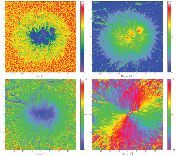
Figure 1: Structure of the magnetic field and the temperature of a relatively symmetric sunspot recorded by the Hinode/SOT-SP on January 2007 which scanned the sunspot area from 12:36 UT to 13:00 UT. Plotted are maps of the (a) temperature, (b) field strength, (c) field inclination and (d) azimuth. The fine-scale structures of this sunspot have been analysed by Tiwari et al. (2013) and van Noort et al. (2013).

Sunspots are often preceded, accompanied and followed by “faculae” (called “plage” at chromospheric levels) which have a spatially averaged field strength of typically between 100 G and 500 G (Title et al., 1992) and are composed of magnetic elements of a range of sizes, with comparatively field-free or weak-field gas in between. Faculae tend to surround and generally outlive the sunspots by a significant amount. Consequently, an old AR is generally composed of faculae only which then decay and disperse to form enhanced network fields. The flux in ARs that is not in the form of sunspots is concentrated in either pores or magnetic elements. The properties of pores include diameters of some Mm and field strengths of 1 kG to 2 kG (Thomas and Weiss, 2004; Sobotka et al., 2012). Magnetic elements have diameters smaller than $\approx$ 350 km and exhibit field strengths of 1 kG to 2 kG (Stenflo, 1973; Rabin, 1992; Rüedi et al., 1992). They are the chief magnetic constituents of faculae, are bright (i. e., hotter than their surroundings) particularly in the mid-photosphere and above (see reviews by Solanki, 1993; Solanki et al., 2006) and are present even in the internetwork (Lagg et al., 2010).

Sooner or later, larger magnetic features (e. g., sunspots) break up and dissolve, their fragments becoming subject to transport and distortion by the convective flows. The smallest and most dynamic convective elements in the QS are granules. Granules have typically diameters of 500 km to 1.5 Mm, a single turnover time of a few minutes and lifetimes of minutes (Nordlund et al., 2009; Zhou et al., 2010). Roughly, the turnover time is the time it takes for hot matter to be transported up through the solar surface, cooled there and transported down again in an intergranular lane, while the lifetime is the time over which a given granule maintains its identity (e. g., in a series of images of the solar surface). In the QS, the magnetic field is additionally swept to the edges of supergranular cells (for a review see Rieutord and Rincon, 2010) with typical diameters of 20 Mm to 30 Mm. This happens on a timescale of several hours and leads to the formation of a patchy magnetic network outlining the boundaries of the supergranular cells.

The transport of magnetic flux to the edges of the granular and supergranular cells leads to an enhancement of magnetic flux if the accumulated flux is of the same polarity. Only when magnetic elements of opposite polarity meet, do they (partially) cancel. In fact, the most significant process of disappearance of magnetic flux appeared to be the cancellation of magnetic elements of opposite polarity (Livi et al., 1985). Wang et al. (1988) concluded that the flux cancellation occurs as a consequence of magnetic reconnection in or above the photosphere, which is likely due to the expansion of the field, so that the opposite polarities meet mainly in the upper photosphere (Cameron et al., 2011). However, a recent study of Lamb et al. (2013) suggests that at least in the QS, flux dispersal is the more common route by which magnetic elements are destroyed, although the exact physical process of flux removal could not be studied (dissipation at small spatial scales is likely to play a role). Another explanation for the apparent disappearance of magnetic flux is that the continuous buffeting of the magnetic flux concentrations leads to the fragmentation of some of the flux into entities whose lesser magnetic flux may then be below the detection threshold of a particular instrument (Berger and Title, 1996).

1.1.5 Relative importance of magnetic forces

Typical values for the particle number density in the solar photosphere are on the order of $n\approx 10^{23}$ m^-3 (at the temperature minimum; Foukal, 2004). Typical quiet-Sun and active-region magnetic field strengths cover the range 100 G to 2 kG. As a consequence, the ratio of the plasma pressure to the magnetic pressure (usually referred to as plasma-$\beta$, or simply denoted by $\beta$) is on the order of 1 to 10 (when averaged over larger regions, Gary, 2001). Note that a value of $\beta\gtrsim 1$ implies that the pressure exerted by the plasma is higher than that exerted by the magnetic field, i. e., that the plasma motion controls the dynamics (and the photosphere is therefore generally said to be “non force-free”). Locally, however, due to the evacuation of magnetic features values of $\beta<1$ are often found. Consequently plasma pressure forces might not be dominant everywhere in the photosphere. Sunspots and kG magnetic elements (for instance at supergranular boundaries) likely represent such exceptions (Priest, 1982).

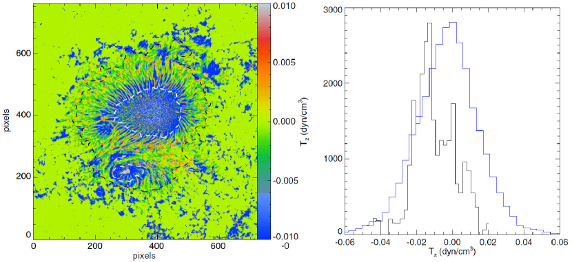
Figure 2: (a) Map of the vertical tension force ($T_{z}$) of an active-region sunspot. Gray and black dashed lines outline the boundaries of the umbra and penumbra, respectively. $T_{z}$ has high negative values at most places over the sunspot. (b) Histograms of $T_{z}$ in the umbra (black) and penumbra (blue). The histogram peak for the umbral field is shifted towards higher negative values, i. e., the umbral field is more force-free than that in the penumbra. (Adapted from Figure 2 of Tiwari (2012). © AAS. Reproduced with permission.)

Solanki et al. (1993) found that in the layers of sunspots near the bottom of the photosphere, $\beta$ is likely above unity everywhere. It was found to drop from higher values in the umbral center and to reach $\beta\approx 1$ at the umbral boundary, followed by another increase towards the outer penumbral boundary. In contrast, Mathew et al. (2004), who used the same spectral lines as Solanki et al. (1993), presented a case where both, the entire umbra as well as the inner penumbra of a sunspot had a $\beta$ slightly below unity. More recently, Tiwari (2012) statistically addressed this topic using high-resolution magnetic field information for 19 sunspots. He found that in mid-photospheric layers most of the fine structures over most of the sunspot areas were nearly force-free with the tendency that umbral fields were less forced, while penumbral fields were more (see Fig. 2). This combination of large plasma-$\beta$ in a spatially averaged sense and small values of $\beta$ locally has important consequences. A comparatively low $\beta$ inside strong-field features helps to explain why they maintain their identity for often considerable lengths of time. The high average $\beta$ implies that magnetic features as a whole, more or less passively, follow convective motions. That in turn explains that the magnetic field in the corona can become tangled and complex (see section 4).

The relative importance of magnetic forces in entire ARs were also estimated. Metcalf et al. (1995) found a value of $\simeq 0.4$ for the net Lorentz force (i. e., the ratio of the total vertical Lorentz force and magnetic pressure force, integrated over the area of the considered AR) and concluded that the analysed AR cannot be validly considered as to be force-free at a photospheric level. In contrast, Gary et al. (1987) found that another analysed AR was indeed force-free, except for some, localized areas (areas for which flaring activity was noticed). Moon et al. (2002) analysed the forces within three flare-productive ARs and found a median of $\approx 0.1$ for the net vertical Lorentz force and argued that the magnetic field at photospheric levels may not be as far from being force-free as commonly assumed. (See also section 5.2.5, for a discussion on the force-freeness of quiet-Sun regions.)

The above compilation shows that the findings, so far, are not entirely conclusive regarding how close to being force-free the photospheric magnetic field really is, they rather show that the amount of forcing (by the gas) depends on the situation being considered. Therefore, special care is required when using photospheric vector magnetic field data as input for, e. g., coronal magnetic field models. Such modelling often relies on routine measurements of the magnetic field, which are to date predominantly performed at photospheric levels (see section 2).

1.2 Chromosphere

The chromosphere lies on top of the photosphere with a thickness of about 1 Mm to 2 Mm, starting from the temperature minimum in traditional one-dimensional model atmospheres. In reality, the chromosphere is far more complex and its thickness is likely to vary strongly from one horizontal location to another. Importantly, it should be thought of more as a temperature rather than a static height regime, with the temperatures increasing from the temperature minimum to $\approx$ $10^{4}$ K (Stix, 2002). Sketches indicating the rich variety of phenomena in the chromosphere and its complexity have been presented in reviews b Wedemeyer-Böhm et al. (2009) and Rutten (2012). Just as the small-scale dynamics of the photosphere are dominated by granular convection, those of the chromosphere are dominated by waves. In internetwork regions these are mainly acoustic waves with a three-minute period, produced in the convection zone (for reviews see Rutten and Uitenbroek, 1991; Carlsson and Stein, 1997; Wedemeyer et al., 2004). But there is also mounting evidence of MHD waves in the chromospheric layers of magnetic structures (Hansteen et al., 2006; De Pontieu et al., 2007).

1.2.1 Characteristic chromospheric magnetic structures

The enhanced magnetic flux concentrations outlining the supergranular cells (the magnetic network) in the photosphere coincide with the bright network seen in chromospheric spectral lines (e. g., of Ca ii). The spatial agreement results from the fact that the magnetic features are nearly vertical (Martínez Pillet et al., 1997; Jafarzadeh et al., 2014b), which is the result of the large field strength of the photospheric ($\approx$ kG) flux tubes. Strong fields produce nearly evacuated structures which result in the flux tubes being buoyant (Parker, 1955) and therefore cause a radial (i. e., vertical) orientation of the field. The vertical orientation is maintained also in the presence of horizontal granular flows (Schüssler, 1984) which bend the magnetic elements (Steiner et al., 1996). The magnetic elements appear bright in chromospheric radiation and larger in size than in the photosphere (Gaizauskas, 1985). Smaller magnetic features are brighter than their surroundings in photospheric radiation due to the vertical, evacuated structures being less opaque than their surroundings. As a consequence, the radiation from the flux tube’s walls may penetrate deep into the thin flux tube’s interior which then appears bright (Spruit, 1976, and for reviews see Solanki (1993) and Steiner (2007)). To explain the enhanced brightness in the chromosphere, however, additional sources of heating, such as the dissipation of waves propagating along the field lines (Roberts and Ulmschneider, 1997) are necessary.

Both in active-region plage and in the network, the kG magnetic field structures appear more diffuse in the chromosphere than in the photosphere (Jones, 1985; Petrie and Patrikeeva, 2009). While the photospheric field is mainly radially oriented, the chromospheric field expands in all directions, forming a magnetic canopy (Giovanelli, 1980; Jones and Giovanelli, 1982), which is likely to be a natural consequence of the excess heating inside magnetic elements (Solanki and Steiner, 1990). Choudhary et al. (2001) compared LOS chromospheric magnetic field as observed in the Ca ii 8542 Å spectral line with a current-free magnetic field model. The latter was based on photospheric LOS magnetic field observations in the Fe i 8686 Å spectral line. Analysing 137 ARs, they found that the chromospheric observations were reproduced best by a current-free model field at a height of $\approx$ 800 km above the photosphere, in agreement with the expected formation height of the Ca ii 8542 Å line. Their results also suggested a decreasing correlation between the observed and modelled LOS magnetic field with increasing field strength, which they attributed to change of the spectral line’s formation height in strong-field regions (although a real deviation from a potential configuration remains a possibility).

On larger (active-region) scales, often observed as dark elongated features in H$\alpha$ 6563 Å and He i 10830 Å images are filaments (“prominences” when observed above the limb; for reviews see Labrosse et al., 2010; Mackay et al., 2010). Filaments straddle polarity inversion lines and typically exhibit heights of $\approx$ 50 Mm, lengths of $\approx$ 200 Mm and a thickness of a few Mm (Stix, 2002). They are involved in many eruptive processes (“eruptive” filaments), but outside of ARs often persist for a long time in the QS (“quiescent” filaments). As suggested by the name, active-region filaments concentrate around the activity belt, while quiescent filaments can be located everywhere on the Sun. In principle, they are thought to be comparatively cool ($T\lesssim 10^{4}$ K) chromospheric material suspended in the corona, sustained by the geometry of the magnetic field. Early investigations of large samples of polar prominences (quiescent as well as eruptive) mainly based on Hanle effect measurements, revealed characteristic longitudinal field strengths on the order of 1 G to 10 G (Leroy, 1977; Leroy et al., 1983; Athay et al., 1983). For active-region filaments, the interpretation of the Zeeman effect revealed strengths of some 100 G to 1 kG for the vertical as well as horizontal field (Lites, 2005; Kuckein et al., 2012; Xu et al., 2012). Xu et al. (2012) were furthermore able to trace the photospheric and chromospheric signatures of the same active-region filament, and detected differing morphologies. This led them to suggest that an emerging magnetic flux rope may, besides sustaining filament material at low atmospheric heights (upper photosphere to low chromosphere), at the same time be able to store plasma at the top part of the flux rope, i. e., at greater (mid chromospheric) heights.

On smaller scales, around sunspots, a radially outward directed filamentary pattern is observed, persisting for hours to days, the sum of which is called the (chromospheric) “super-penumbra” (Hale, 1908b). These structures are seen in almost all chromospheric spectral lines, including H$\alpha$ 6563 Å, Ca ii 8542 Å and Ly$\alpha$ 1216 Å and, though more rarely, also in Ca ii H and K (see Pietarila et al., 2009, and references therein). A common assumption is that these chromospheric “fibrils” outline the direction of closed magnetic field structures in the upper photosphere and chromosphere, linking the spot with the surrounding flux of opposite polarity (Nakagawa et al., 1971; Woodard and Chae, 1999), allowing a mass flow away from the spot (Evershed, 1909) or into the spot (“inverse Evershed effect”; St. John, 1913, and for a review see Solanki (2003)). In a similar fashion, fibrils (seen, e. g., in H$\alpha$) are thought to connect opposite polarity magnetic flux elements in the QS (Reardon et al., 2011; Beck et al., 2014), although some fibrils may follow the chromospheric part of magnetic field lines that continue into the corona (see also section 5). The fibril pattern around sunspots is often observed to be oriented radially outwards and forming whirls which exhibit rotation patterns specific to the hemisphere where they are observed (Hale, 1908a; Richardson, 1941; Peter, 1996). Vecchio et al. (2007) underlined the likeliness of fibril-like structures seen in Ca ii 8542 Å images to outline the canopy at chromospheric levels. The fibrils are thought to follow the canopy magnetic field of sunspot super-penumbrae, whose base rises slowly from the edge of the spots as one moves radially outward alongside a decreasing magnetic field strength (Giovanelli, 1980; Giovanelli and Jones, 1982; Solanki et al., 1994, and see also section 1.3.1).

1.2.2 Indirect tracing of chromospheric fields

Woodard and Chae (1999) investigated the non-potentiality of fibril structures in the QS. They performed a comparison of field lines from a potential field model with fibrils observed in H$\alpha$ 6563 Å. They found, under the assumption that the fibrils trace magnetic field lines, that the observed fibril structure aligns well with the magnetic field model in some places, but in others not (see Fig. 3a). They concluded from this finding that the quiet-Sun’s chromospheric magnetic field is far from a potential state (i. e., it carries currents on small scales). This interpretation has been tested for active-region fibrils by Jing et al. (2011) who based their study on a potential magnetic field model starting from chromospheric magnetograms. Again it was found that in some places the modelled horizontal field agrees well with the segmented fibril orientation but in other places not (Fig. 3b). It appeared that there is a link between the horizontal shear of the involved field and the mismatch between model and observation: the higher the shear of the observed chromospheric magnetic field structures, the lower the agreement with a potential magnetic field model. Consequently, potential field models, either based on photospheric or chromospheric magnetic field data, can in general not be assumed to adequately reproduce the (chromospheric) magnetic field, assuming that fibrils indeed outline the orientation of the chromospheric magnetic field.

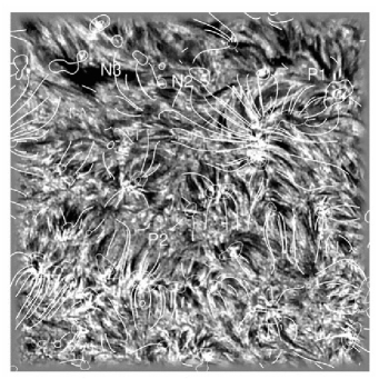
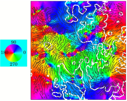
Figure 3: (a) Comparison of H$\alpha$ fibrils (observed at 6563 Å; gray-scale background) with projections of potential magnetic field lines over-plotted. The FOV spans roughly $300\mbox{${}^{\prime\prime}$}\times 300\mbox{${}^{\prime\prime}$}$. Except for some local areas denoted as P1 and P2 (upper right and lower middle part of the image, respectively), poor agreement between filed and the direction of fibrils is recognized in particular around N1, N2, and N3 in the upper mid to left part of the frame. (Figure 2 of Woodard and Chae (1999). With kind permission from Springer Science and Business Media.) (b) Comparison of H$\alpha$ fibrils (at 6563 Å; black curves) with the chromospheric potential magnetic field azimuth, counted counter-clockwise from 0^∘ at solar west. The white contours outline magnetic PILs. The FOV is roughly $254\mbox{${}^{\prime\prime}$}\times 264\mbox{${}^{\prime\prime}$}$. Good agreement is found between the potential field azimuth and the fibril orientation in some places, while a clear deviation of the two direction is seen in others. (Adapted from Figure 5 of Jing et al. (2011). © AAS. Reproduced with permission.)

An alternative interpretation of the results of Woodard and Chae (1999) and Jing et al. (2011) is that fibrils do not outline the orientation of the chromospheric magnetic field. This, however, is in direct contrast with the results of recent numerical simulations which suggested that H$\alpha$ fibrils are visible manifestations of high-density ridges aligned with the magnetic field (Leenaarts et al., 2012), thus serving as an indirect tracer of the vertical-to-horizontal transition of the magnetic field orientation around magnetic flux concentrations. This was addressed by de la Cruz Rodríguez and Socas-Navarro (2011) who compared the observed orientation of fibrils in Ca ii 8542 Å images to the chromospheric magnetic field vector, inferred from observed polarization signals originating from the same spectral line. They found that most of the fibrils in the surrounding of a penumbral boundary nicely followed the magnetic field direction but also recorded a significant mismatch for a considerable number of fibrils (Fig. 4a). They also noted a too rapid decrease of the linear polarization signal when moving out of the penumbral area, if the fibril pattern indeed were to outline the super-penumbral field direction. The rapid decrease of the linear polarization signal, however, may be attributed to the height of the canopy base relative to the formation height of the spectral line. This was re-addressed recently by Schad et al. (2013) who, in contrast to de la Cruz Rodríguez and Socas-Navarro (2011), found a clear coincidence of the projected direction of super-penumbral fibrils and the inferred magnetic field (to within $\pm 10^{\circ}$) using He i 10830 Å observations. They detected a notable change of the inclination only close to where the fibrils turn towards their rooting point in the sunspot (Fig. 4b). Moreover, based on their findings, they explicitly support schemes which propose the inclusion of the spatial information delivered by chromospheric fibril observations to increase the success of force-free coronal magnetic field models. Such proposed schemes use the fibril information to increase the match between the modelled and observed horizontal field at chromospheric heights (where the magnetic field vector is not routinely measured; see Wiegelmann et al., 2005a, 2008; Yamamoto and Kusano, 2012).

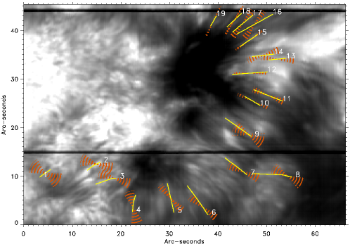
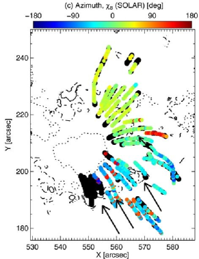
Figure 4: (a) Comparison of visually determined directions (yellow lines) of Ca ii fibrils (observed at 8542 Å; gray-scale background) to the magnetic field azimuth compatible with linear polarization signals (orange cones). While the fibril orientation is picked up by the reconstructed horizontal magnetic field orientation for a fair number of fibrils (e. g., fibrils 9 to 19), it is only poorly recovered for others (e. g., fibrils 1 to 5). (Figure 1 of de la Cruz Rodríguez and Socas-Navarro (2011). Reproduced with permission from Astronomy & Astrophysics, © ESO.) (b) Spatial map of the magnetic field azimuth along selected super-penumbral fibrils, inferred from He i at 10830 Å observations. The dotted and dot-dashed contours indicate a photospheric magnetic field inclination of 135^∘ and 90^∘, respectively. Black dots mark severe deviations between the inferred and observed fibril orientation. They are restricted to where fibrils turn to their photospheric rooting points. (Adapted from Figure 10 of Schad et al. (2013). © AAS. Reproduced with permission.)

1.2.3 Plasma-$\beta$ in the chromosphere

Density and temperature are heavily structured in the highly dynamic chromospheric environment so that the relative strength of the plasma pressure and magnetic forces also varies strongly with position, at a given height. The height at which the magnetic forces start to dominate over others (i. e., where $\beta<<1$) is expected to be strongly corrugated relative to the solar surface. In the QS, that height is expected to vary between $\approx$ 800 km and 1.6 Mm above the photosphere (Rosenthal et al., 2002). In ARs, this height is likely to be lower, as shown by Metcalf et al. (1995). They used chromospheric vector magnetic field measurements inferred from observations in the Na i 5896 Å spectral line to test the relative contribution of the plasma pressure and magnetic forces in an AR. They found that the atmosphere above that AR could be considered to be force-free from $\approx$ 400 km above the solar surface. Gary (2001) was able to confirm that finding by combining a plasma pressure and magnetic field model to estimate the pattern of interchanging dominance of plasma and magnetic pressure with height in the solar atmosphere (see Figure 5). He concluded that the magnetic forces above sunspots should start to dominate from relatively low heights ($\gtrsim$ 400 km above the photosphere). Above plage regions, the model results suggest this to be true from $\gtrsim$ 800 km above a photospheric level upwards. In summary, ARs can be considered to be force-free in most of the chromosphere (in contrast to quiet-Sun areas; see section 5.2.5).

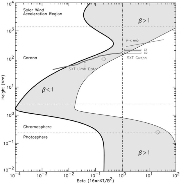
Figure 5: Distribution of the plasma-$\beta$ as a function of height above an AR. The shaded area represents the vertical run of $\beta$ for open and closed fields originating between a sunspot (represented by the thin solid line) and a plage region (represented by the thick solid line). $\beta$ becomes only small ($\simeq 10^{-2}$) at heights above the upper chromosphere and mid corona. Note that this low-$\beta$ region is sandwiched between high-$\beta$ regions (the photosphere and low to mid chromosphere below as well as the upper corona and solar wind acceleration region above). (Figure 3 from Gary (2001). With kind permission from Springer Science and Business Media.)

1.3 Magnetic coupling from the lower solar atmosphere to the corona

1.3.1 Magnetic canopy

At photospheric levels only a small fraction of the solar surface is occupied by strong magnetic field ($\lesssim 5$%). In contrast to that, the coronal magnetic field fills the entire coronal volume and is distributed relatively uniformly in strength (although not in orientation). Consequently, the photospheric field must spread out with increasing height in the solar atmosphere. The magnetic field expands until it either turns over and returns to connect back to the photosphere or it meets the expanding field of the neighbouring flux tubes. It then forms a “magnetic canopy”, i. e., a base almost parallel to the solar surface and overlying a nearly field-free atmosphere (see Fig. 6). For a comprehensive review of the current picture of the magnetic coupling of the photosphere, chromosphere and transition region to the corona we refer to Wedemeyer-Böhm et al. (2009) and restrict ourselves to a brief summary here. Estimates for the merging height of photospheric flux tubes range from some 100 km for active-region to $\approx$ 1 Mm for quiet-Sun magnetic fields (Spruit, 1981; Giovanelli and Jones, 1982; Roberts, 1990). (Note that these estimates essentially depend on the filling factor, i. e., whether the considered region exhibits a high or low mean magnetic field strength.)

Figure 6: Sketch of the quiet-Sun magnetic field structure in a vertical cross section through the atmospheric layers of the Sun. Swept to the edges of supergranular cells by large-scale convective flows (thick, large arrows at bottom), intense magnetic network elements or sunspots form. Small-scale convective flows (thin, small arrows below dotted horizontal line representing the photosphere) result in the photospheric granular pattern. The magnetic field lines (solid lines) expand at chromospheric heights and form the nearly horizontal magnetic canopy (dashed line). (Adapted from Judge (2006) and Wedemeyer-Böhm et al. (2009).)

The expansion of the magnetic field with height is a consequence of the small gas-pressure scale height ($\approx$ 100 km in non-magnetic regions; Durrant, 1988). From the lateral pressure balance follows that the field strength must rapidly decrease with height. (Remember that lateral pressure balance requires the gas pressure inside a flux tube to be lower than outside it.) With increasing height, the magnetic field strength drops due to the fall-off of the gas pressure and flux conservation implies that the magnetic field must spread out, i. e., the extension of the magnetic structures must increase rapidly. Since magnetic features are hotter than their surroundings in the middle/upper photosphere and chromosphere, the internal gas pressure drops more slowly with height than the external gas pressure. As a consequence, at certain heights, the internal pressure force exceeds the external. This removes the lateral confinement of the magnetic structures and allows the structures to expand unhindered, until it hits field from another photospheric source. This implies a significant horizontal component of the field over a large part of the volume (the canopy; Solanki and Steiner, 1990; Bray et al., 1991). The different merging heights thus depend, besides on the distance between neighbouring magnetic features, on the temperature difference between the magnetic field structures and their surroundings, causing successively lower canopy heights for increasing temperature differences (see chapter 5 of Aschwanden (2005)). Above this merging height the magnetic field becomes increasingly homogeneous. Generally, the field of a magnetic element is seen to be shaped roughly like a wine glass. The direction of the field then depends on the structure of the magnetic field in its surroundings and the connectivity of the field lines on a larger scale (i. e., whether they are closed or open and where they return to the solar surface).

In plage regions, the flux tubes merge already in the mid to upper photosphere, so that the atmosphere above is almost fully magnetic (Buente et al., 1993). Model results suggested that, in the QS and in CHs where magnetic features are further apart, this base is located somewhere in the lower chromosphere (Gabriel, 1976; Jones and Giovanelli, 1982; Solanki and Steiner, 1990; Solanki et al., 1991). Quite some time after the first speculations on the height of canopy-type magnetic fields, observational evidence for the merging heights in plage of on the order of several hundreds of km have been delivered (Steiner and Pizzo, 1989; Guenther and Mattig, 1991; Bruls and Solanki, 1995). Rosenthal et al. (2002) performed numerical simulations of the propagation of waves through a model atmosphere, resembling properties of the chromospheric network and internetwork, and found the canopy height to vary between $\approx$ 800 km and 1.6 Mm above the base of the photosphere. However, a considerable number of findings, especially in the QS, led to serious doubts upon the reality of a large-scale, undisturbed magnetic canopy there (for details see section 5.2.1).

Even though some aspects of the magnetic canopy, especially in the QS are still to be elaborated further, its basic nature seems clear: it is not a simple, rigid structure and also not at a constant height in the solar atmosphere. Instead, its shape and height is different for regions on the Sun with different amounts of magnetic flux and it also varies with time. Above the canopy, the coronal volume is filled more or less uniformly with magnetic field.

1.4 Corona

1.4.1 Transition region and coronal base

The corona is to be thought of as a temperature regime, covering a few times $10^{5}$ K in open field regions (such as CHs; see section 6), $\approx$ 1 MK to 2 MK (megakelvin) in the predominantly closed field of the quiet-Sun corona, and up to 2 MK to 6 MK in ARs (see chapter 1 of Aschwanden, 2005). It even can briefly reach values of 10 MK to 20 MK during strong flares. It spans the atmospheric layers between the transition region (within which the temperatures increase from $\approx$ $10^{4}$ K to $\approx$ 1 MK) and the height where the solar wind is accelerated, i. e., spanning several hundreds of Mm in height (Gary, 2001). The very narrow transition region not only bridges a large difference in temperature, but also separates the dilute coronal plasma (with number densities of $n\lesssim 10^{12}$ m^-3) from the dense ($n\gtrsim 10^{16}$ m^-3) chromosphere (see chapter 1 of Aschwanden (2005)). The base of the corona is not to be thought of as a horizontal layer somewhere above the solar surface. As the thickness of the chromosphere beneath varies, so does the height of the coronal base above the solar surface (see section 1.3 for details).

1.4.2 Morphology of coronal magnetic fields

Two very distinct magnetic configurations are present in the corona. The field is either arranged in the form of closed loops of enhanced emission, or in the form of open field lines seemingly not connecting back to the solar surface (Schrijver et al., 1999; Solanki et al., 2006). Arcades (ensembles) of bright coronal loops connect regions of opposite magnetic polarity on the solar surface and are often, but not necessarily always, rooted in an AR. Large-scale loop systems (sometimes exhibiting sigmoidal shapes) are often found to connect neighbouring ARs and/or ARs with their quiet-Sun surrounding (Strong and et al., 1994). Following Reale (2010), the observed coronal loop systems span a wide range of length scales, from a few Mm (bright points) up to giant arches which may span 1 Gm (gigameter). Several loop arcades neighbouring each other are often found in magnetically complex ARs and often host eruptive processes such as flares or CMEs (see section 4). Therefore, in the majority of cases, bright coronal loops (see section 4.1 for more details) are concentrated around the activity belts.

Most of the quiet-Sun magnetic field (see section 5) that reaches the corona is rooted in the magnetic network. At greater heights, they fan out to form funnels and to fill the coronal volume above (Gabriel, 1976; Dowdy et al., 1986). Along the open field structures, plasma is efficiently transported outwards, which allows charged particles to escape from the solar atmosphere. Especially during solar activity minimum, open magnetic flux is concentrated around the poles, causing depleted regions which emit less than their surrounding temperatures above 1 MK and consequently appear dark in coronal images (therefore termed “coronal holes”; see section 6). At lower latitudes the coronal structure is dominated by “helmet streamers” and “pseudo streamers”, extending out to several solar radii in height (Schwenn, 2006). Helmet and pseudo streamers are visible as enhanced emission in the form of a cusp above the limb, bridging the space between open fields of opposite and same polarity, respectively (see Pneuman and Kopp (1971) and Wang et al. (2007), respectively.

2 Magnetic field modelling

The solar magnetic field is routinely measured mainly in the photosphere, whereas direct measurements in the higher solar atmosphere are available for individual cases. If the 3D magnetic field vector in the chromosphere and corona were to be measured routinely with high accuracy, cadence and resolution, indirect modelling approaches (as discussed in the following sections) would not be required. Since this is not yet the case (see section 2.1), modelling approaches of different sophistication have been developed with the aim of computing the magnetic field in the upper solar atmosphere, generally starting from measurements made in the lower atmosphere.

One possibility is to use the longitudinal photospheric magnetic field component, or the measured full magnetic field vector (if available) as boundary condition for force-free magnetic field reconstruction techniques. This is possible since the solar corona is almost force-free, because the magnetic pressure is several orders of magnitude higher than the plasma pressure. That allows neglecting nonmagnetic forces to lowest order and applying such methods (see section 2.2). Because these models are snapshots and assume stationarity and stability of the coronal magnetic field configuration, they are not to be used for modelling of dynamic features (such as CMEs, flares or eruptive prominences). Moreover, these models do not provide a self-consistent description of the coronal plasma. Time-dependent simulations are required for these aims, usually within the MHD approach (see section 2.3). Full MHD models (see section 2.3.1) are both theoretically and observationally very challenging because plasma and magnetic field have to be modelled self-consistently.

Complementary to these numerical approaches one can use the fact that the emitting coronal plasma (as visible in coronal images; see section 4.1) is frozen into the magnetic field and consequently the coronal loops visible in the images outline magnetic field structures. Therefore coronal images can be used to identify the 3D shape of the magnetic field structures when images from multiple viewpoints exist (e. g., from the STEREO-spacecrafts, SOHO or SDO). A 3D reconstruction of structures seen above the solar limb can be performed by stereoscopic and tomographic methods (see section 2.4.1 and 2.4.2, respectively). Coronal images are also frequently used to validate the results of coronal magnetic field models. In some cases, time sequences of coronal images show oscillating coronal loops, which allow estimating the coronal magnetic field strength by coronal seismology (see section 2.4.3).

The main aim of this section is to give a short overview of the methods for deriving the 3D magnetic field structure of the upper solar atmosphere (although we start this section with a short review of direct measurements of chromospheric and coronal magnetic fields). We refer to specialized reviews and the primary literature for further details. Outside the scope of the present review are methods of the interaction of the convection zone with the solar atmosphere by flux emergence (the interested reader can find a recent review on the theory of flux emergence in Cheung and Isobe, 2014). Methods to analyse the 3D coronal magnetic field topology are described in section 4.2 and also in a review by Longcope (2005).

2.1 Direct coronal magnetic field measurements

Direct measurements of the solar magnetic field are an important tool for understanding the magnetic field in the upper solar atmosphere. Here, we briefly introduce the most important methods for measuring the chromospheric and coronal magnetic field directly. The difficulties of performing such measurements are only briefly touched upon here (for details see Raouafi, 2005; White, 2005; van Driel-Gesztelyi and Culhane, 2009; Cargill, 2009). Thanks to instrumentation, e. g., the ground-based NSO/DKIST (planned to become operational in 2019), together with powerful inversion techniques, coronal field measurements might become a prosperous method in future.

2.1.1 Chromospheric magnetic field measurements in the infrared

Infrared lines have been used to derive the magnetic field vector near the coronal base in the upper chromosphere. Initial measurements of the LOS magnetic field were performed by Harvey and Hall (1971), Rüedi et al. (1995) and Penn and Kuhn (1995) and the first vector magnetic field measurement by Rüedi et al. (1996). Solanki et al. (2003) applied the same method using the He I 10830 Å line, which is optically thin. Consequently, the measurements are related to different formation heights, following the fluctuating height of the coronal base. The authors managed the 3D structure of the chromospheric loops to be reconstructed by applying the following criteria. If a randomly selected pixel matches in field strength and direction the two neighbouring pixels, then the radiation is assumed to originate from the same loop. Because the full magnetic field vector is inferred, this allows to reconstruct the loop in 3D, with the additional constraint that the field strength decreases with height. The 3D structure deduced for the emerging loops was questioned by Judge (2009) but it was later shown by Merenda et al. (2011) that the proposed geometry provided a better representation to the data than the flat alternative proposed by Judge (2009). Simultaneously with these chromospheric measurements, the photospheric field vector was measured as well, and extrapolated into the chromosphere using force-free modelling techniques (see section 2.2), where the NLFF model was found to agree best with the chromospheric observations (for details see Wiegelmann et al., 2005b).

2.1.2 Coronal magnetic field measurements in infrared

Coronal measurements in the infrared are possible from the ground with a coronagraph, or with instruments from space. An overview on some aspects of the usage of infrared lines to measure the coronal magnetic field can be found in Penn (2014). That review also gives a detailed discussion of advantages and disadvantages of using infrared lines in general (not restricted to coronal magnetic fields). More than ten coronal lines in the infrared have been identified and some of them are magnetically sensitive. The Fe xiii 10750 Å line, for instance, has been used to measure the Stokes vector in the corona, which in principle would allow determining the magnetic field vector by an inversion. A general problem with coronal observations is, however, that due to the optically thin coronal plasma, any recorded radiation form the corona is integrated over the LOS. This naturally complicates the interpretation of the measurements, so that to derive the spatially resolved coronal magnetic field vector in 3D, measurements from multiple viewpoints are necessary. The situation has some similarities with deriving the coronal density by a tomographic inversion (see section 2.4).

Figure 7: (a) Full-disk NRH radio emission observed on June 27, 2004 at 432 MHz and (b) GOES/SXI X-ray emission. The close relationship between the radio and X-ray emission can be seen in the form of bright emission around ARs and minimal emission in CHs. (Adapted from Figure 5 of Mercier and Chambe (2012). Reproduced with permission from Astronomy & Astrophysics, © ESO.)

2.1.3 Coronal magnetic field measurements at radio wavelengths

Radio signatures emitted from the active-region corona, currently represent the most widely used direct measure of the magnetic field. Because they are produced only in specific circumstances when electrons are guided by a magnetic field, they allow the reconstruction of the magnetic field strength in the corona (White et al., 1991; Schmelz et al., 1994; White and Kundu, 1997; Brosius et al., 1997; Lee et al., 1998, 1999). Note that hard X-ray emission often goes hand in hand with radio emission since the efficient emission of both requires electron energies of $\gtrsim 10$ keV (see Figure 7 and the review by White et al., 2011). Information on the height of the on-disk radio source in the corona is not accessible through such measurements, except occasionally for coronal structures at different heights above the solar limb using near infrared wavelengths (Arnaud, 1982a, b; Lin et al., 2000, 2004) or radio observations (Brosius and White, 2006). For on-disk measurements, the lacking height information may be compensated by (force-free) magnetic field modelling of the coronal structure, starting from photospheric magnetograms (Liu and Lin, 2008; Bogod et al., 2012; Kaltman et al., 2012). Furthermore, radio maps can be used also for a stereoscopic 3D reconstruction (see section 2.4.1).

2.2 Force-free modelling from photospheric measurements

The solar magnetic field vector is measured routinely with high accuracy only in the photosphere, e. g., by SDO/HMI at a constant resolution of $1\mbox{${}^{\prime\prime}$}$ over the whole solar disk. Under reasonable assumptions we can extrapolate these photospheric measurements into the higher solar atmosphere, where direct magnetic field measurements are more challenging (see section 2.1). So, which assumptions are reasonable in the solar atmosphere? A key to answering this question is the comparison of magnetic and non-magnetic forces and in particular the plasma-$\beta$. While the plasma-$\beta$ is around unity in the photosphere it becomes very small (about $10^{-4}$ to $10^{-2}$) in the corona (at least in ARs; see Figure 5 and section 1.2.3 for details). Consequently non-magnetic forces can be neglected in the low $\beta$ corona, and the coronal magnetic field can be modelled as a force-free field (the Lorentz-force vanishes). The electric current density,

$${\bf j}=\frac{1}{\mu_{0}}\,\nabla\times{\bf B},$$

has either to be parallel or anti-parallel to the magnetic field, leading to

$$\nabla\times{\bf B}=\alpha\,{\bf B},$$

where a positive (negative) value of $\alpha$ means that the electric current flows parallel (anti-parallel) to the magnetic field.

While a low plasma-$\beta$ is a reasonable justification for using force-free models, the opposite is not true. A high (of order one or more) plasma-$\beta$ does not exclude force-free magnetic fields. If the non-magnetic forces compensate each other (e. g.,the plasma pressure gradient is compensated by the gravity force in a magneto-static equilibrium) then the Lorentz force can still vanish, even if $\beta$ is not small. In the general high-$\beta$ case, however, non-magnetic forces have to be considered self-consistently, e. g., in a magneto-static or stationary MHD model. We will only summarize some basics about the possibilities and problems of force-free models and avoid mathematical and computational details. For a more detailed overview on the methods used to compute solar force-free fields see Wiegelmann and Sakurai (2012). Depending on the force-free parameter (or function), $\alpha$, one distinguishes between potential (current-free) fields $(\alpha=0)$, linear force-free fields (LFF; $\alpha$ is globally constant) and the general case that $\alpha$ changes in space, i. e., the nonlinear force-free (NLFF) approach.

2.2.1 Potential and linear force-free fields

The simplest case, a potential field, requires only the LOS photospheric magnetic field component as boundary condition. Current-free equilibria are mathematically simple and represent the lowest possible energy state of a coronal magnetic field. For computations on a global scale (PFSS models), one assumes that all field lines become radial at the “source surface” (at about 2.5 solar radii; see Schatten et al., 1969, for details). Potential field models are popular because they are easy to compute and are capable of reproducing the basic coronal magnetic field structure. More sophisticated methods (as discussed in the following) are numerically expensive and often use a current-free field solution as initial guess for an iteratively sought, non-potential solution.

In order to employ a LFF magnetic field model, only the photospheric LOS magnetic field component is required as well, but such models contain one additional free parameter $(\alpha)$. The value of $\alpha$ (constant in space) can be inferred from additional observations, e. g., in the form of an average value of the entire photospheric distribution of $\alpha=(\nabla\times{\bf B})_{z}/B_{z}$. Note that $\alpha$ is the ratio of the vertical (LOS) current density and the vertical (LOS) magnetic field magnitude, and that the vertical (LOS) current density can be derived from the horizontal (transverse) magnetic field. (In that case, the knowledge of all three vector components of the magnetic field is required.) Alternatively, $\alpha$ can be deduced and/or optimized by the comparison of model magnetic field lines and coronal observations (either directly with coronal loops seen in EUV images, or coronal loops extracted from such images; and see also section 2.4.1).

On global scales, LFF models are mathematically and computationally possible, but are not frequently employed, mainly for two reasons. Firstly, the maximum allowed value of $\alpha$ scales with the inverse of the length scale of the computational domain. Consequently very small values of $\alpha$ are possible but they are so small that they have no significant effect (i. e., the resulting magnetic field is almost similar to a potential field configurations). Secondly, observations show that both signs of $\alpha$ can be present in different regions on the Sun, at the same time. That is a contradiction to the LFF assumption, namely that $\alpha$ is constant (i. e., has the same value for different regions on the Sun).

On smaller scales (in particular to analyze ARs), however, LFF models were used, though more frequently before the time when vector magnetograms started to became routinely available (as provided to date by, e. g., SDO/HMI). On these smaller scales, the maximum value of $\alpha$ can be significantly larger than on global scales and consequently active-region LFF fields can be very different from potential ones, e. g., the associated field lines can be sheared. Also for LFF models employed on active-region scales, however, the observation of different values of $\alpha$ in different portions of the same AR contradicts the basic assumption of a single value of $\alpha$ being representative for the entire AR under consideration.

2.2.2 Nonlinear force-free fields

Given the limitations of potential and LFF approaches (as discussed above) for a meaningful and self-consistent modelling of coronal magnetic fields, one has to take into account that $\alpha$ is a function of position. This spatial dependence is accounted for in NLFF models, which are much more challenging, both mathematically (one has to solve nonlinear equations) and observationally (mostly photospheric vector magnetograms are required as input, instead of just the longitudinal (vertical) field component). Measurement inaccuracies in photospheric vector magnetograms (e. g., due to noisy Stokes profiles and instrumental effects) affect the quality of NLFF coronal magnetic field models. The modelled coronal field, however, is less sensitive to these measurement errors than the photospheric field vector itself (Wiegelmann et al., 2010b). A review on methods for computing NLFF fields has been given by Wiegelmann (2008). The corresponding numerical implementations have been intensively reviewed, and repeatedly evaluated and improved within the last decade (see Schrijver et al., 2006; Metcalf et al., 2008; Schrijver et al., 2008; De Rosa et al., 2009). The numerical schemes have been implemented in cartesian and spherical geometry to perform active-region and global magnetic field modelling, respectively. As boundary condition, either the magnetic field vector at the bottom boundary of the computational domain or, alternatively, the vertical magnetic field and vertical electric current density is usually required.

A difficulty arises from the fact that the plasma in the corona is a low-$\beta$ plasma, but that of the photosphere is not. In the photosphere, $\beta$ is on average of the order of unity or more (Gary, 2001), although locally considerably smaller values may be found (e. g., in the interiors of magnetic elements; see Zayer et al., 1990; Rüedi et al., 1992). Note that a non-vanishing plasma-$\beta$ does not exclude the existence of a force-free field, but one has to be careful when using photospheric measurements as boundary condition for NLFF computations. Because then it cannot be guaranteed that the photospheric magnetic field vector is consistent with the assumption of a force-free field in the corona. One can find out whether the vector magnetic field measurements are consistent by writing the force-free equations as the divergence of the Maxwell stress tensor, integration over the entire computational volume and applying Gauss’ law. For force-free consistency, the value of the resulting surface integrals have to vanish (see Aly, 1989, for details), or in practice must then be sufficiently small. Theoretically, the surface integrals need to be evaluated over the entire boundary of the computational domain, but in practice this is only possible for the the bottom (photospheric) boundary, where the field is measured. This is justified for ARs that are surrounded by weak (quiet-Sun) fields where the gross part of the magnetic flux closes within the AR (i. e., on the bottom boundary) and the contribution of the other boundaries can be neglected.

Only exceptionally, however, active-region vector magnetograms fulfill the force-free criteria (for such an example see Wiegelmann et al., 2012). In the majority of cases, they are not force-free, simply because the photosphere is a non-force-free environment. Additionally, polarization signals are often affected by the temperature in the sampled magnetic features and introduce biases between, e. g., sunspots and magnetic elements forming plage regions (Grossmann-Doerth et al., 1987; Solanki, 1993). To circumvent this problem a procedure dubbed “preprocessing” has been developed. The method uses (force-free inconsistent) photospheric vector field measurements as input and provides a force-free consistent vector field as output (see Wiegelmann et al., 2006, for details). An alternative is to measure the magnetic field vector higher in the solar atmosphere, e. g., in the low-$\beta$ chromosphere (exclusively, or in addition to photospheric measurements).

To our knowledge, the first and so far only NLFF extrapolation from vector magnetograms observed simultaneously at multiple heights (at a photospheric and chromospheric level) have been performed by Yelles Chaouche et al. (2012), in order to study the structure of an AR filament. One difficulty in combining and comparing two such data sets is that the exact height in the atmosphere of the chromospheric measurement is unknown. As a reasonable approximation the authors assumed that the chromospheric measurements refer to the height of best agreement with the NLFF reconstruction based on the photospheric vector field (about 2 Mm above the solar surface surface).

Despite the difficulties discussed above, NLFF extrapolations are a powerful tool for deriving the 3D coronal magnetic field above ARs. On the other hand the applicability of force-free models to quiet-Sun magnetic fields is questionable because it is very likely neither force-free nor quasi-steady (see Schrijver and van Ballegooijen, 2005, and section 5.2.5 for details).

2.3 MHD models

2.3.1 MHD models of the coronal magnetic field

A full understanding of the physical processes in the upper solar atmosphere requires the knowledge of the plasma that populates the investigated magnetic structures. Deriving these properties in the outer solar atmosphere, however, remains a challenging task. Most commonly used models for a self-consistent description of the plasma and magnetic field are based on the MHD approximation. Interestingly, even though the MHD approximation is strictly valid only in collisional plasmas, the collision-free coronal plasma is often modelled using such an approach. More sophisticated, collisionless kinetic models cannot be applied to model large-scale structures in the solar corona since the considered scales are several orders of magnitude larger than the relevant (microscopic) scales which have to be resolved in kinetic simulations (e. g., the gyro-radius or Debye-length). This approach, however, is frequently applied to model the solar wind plasma (see review by Marsch, 2006).

One approach to derive plasma quantities, which can then be compared to observations, is forward modelling aided by time-dependent MHD simulations (see Peter et al., 2006). As an initial state, a potential field is computed from the measured photospheric (LOS or vertical) magnetic field component. (Note that for MHD simulations the magnetic field data has usually to be scaled to a lower spatial resolution.) A strength of the forward MHD modelling technique is that the resulting plasma quantities can be used to compute synthetic spectra, which can be compared with observed chromospheric and coronal images/spectra (e. g. Peter et al., 2006, using SOHO/SUMER EUV data).

2.3.2 MHS models

A simpler approach, when refraining from performing numerically expensive time-dependent MHD simulations is to use a reduced set of equations, e. g., MHS or stationary MHD. This allows a self-consistent modelling of magnetic field and plasma e. g., in the high-$\beta$ regimes containing the photosphere and lower chromosphere, and beyond the source surface in global simulations. Generally, these equilibria require the computation of nonlinear equations, which are numerically even more challenging (and slower converging) than the set of NLFF equations, in particular in a mixed-$\beta$ plasma (see Wiegelmann and Neukirch, 2006; Wiegelmann et al., 2007, for an implementation in cartesian and spherical geometry, respectively).

Mathematically simpler, and computationally much faster, is the subclass of MS models, which are based on the assumption that electric currents flow on spherical shells perpendicular to gravity (resulting in horizontal,i. e., parallel to the lower boundary, currents in cartesian geometry). This approach allows linearizing the MS equations and solving them with a separation-ansatz (see Low, 1991; Bogdan and Low, 1986; Neukirch, 1995, for a cartesian and spherical approach, respectively). Because of the linearity of the underlying equations, a field-parallel electric current can be superposed (for a constant value of $\alpha$). The final current distribution consists of two parts: a LFF one and another one that compensates non-magnetic forces such as pressure gradients and gravity. These classes of MS equilibria require only LOS photospheric magnetograms as boundary conditions, are relative easy to implement and allow the specification of two free parameters (the force-free parameter $\alpha$ and additionally a parameter which controls the non-magnetic forces). The limitations on $\alpha$ are similar to those discussed for LFF modelling approaches (see section 2.2). In these models, plasma pressure and density are computed self-consistently in order to compensate the Lorentz-force. Above a certain height the corresponding configurations become almost force-free, which in principle allows it to model a forced photosphere and chromosphere, together with a force-free corona above. A limitation of MS equilibria is that the two free parameters are globally constant and the method does not guarantee a positive plasma pressure and density. To ensure positive values of these quantities, one either has to add a sufficiently large background atmosphere (which may lead to unrealistically high values of the plasma-$\beta$), or is limited to small values of the parameter controlling the non-magnetic forces. Note that, as force-free approaches, MS models are only snapshots of the coronal field and the temporal evolution of such configurations can only occur as a series of equilibria, in response to temporally changing boundary conditions.

2.3.3 Flux transport models

So far (for the aim of coronal magnetic field modelling) we have discussed only the coronal response to photospheric changes, but did not try to understand the evolution of the photospheric field itself. This can be done on a large (global) scale with the help of flux transport models (Leighton, 1964, and for recent reviews see chapter 2 in Mackay and Yeates (2012) as well as Jiang et al. (2014)). The aim of magnetic flux transport models is to simulate how (newly emerged) flux is transported horizontally on the solar surface, i. e., in the photosphere. The magnetic field is assumed to be radially oriented. The main contributing flows and velocities on large scales are differential rotation and meridional flows. On smaller scales, convective processes on granular and supergranular scales become important too, where the granular scales are generally ignored.

A natural application of flux transport models is to compute the evolution of active-region or global coronal fields (see Sheeley et al., 1987; Baumann et al., 2004), as well as to investigate the development, structure and decay of polar CHs (see Sheeley et al., 1989), and to estimate the Sun’s open magnetic flux. Flux transport computations performed in recent times often start from observed magnetograms, e. g., full-disk (Schrijver and De Rosa, 2003) or synoptic (Durrant and McCloughan, 2004) LOS magnetograms from SOHO/MDI. As a welcome side product, fluxes are obtained also for regions where no LOS measurements can be performed or where they are not reliable (i. e., at the far side and around the poles of the Sun, respectively). Additionally, such computations can be used to compensate gaps in the original full-disk or synoptic LOS data. To our knowledge, current flux transport models provide only the radial component of the photospheric field (i. e., not the full field vector), however.

For the aim of coronal magnetic field modelling, the resulting (synthetic) magnetic flux maps can be used in a similar fashion as LOS magnetogram data. Most popular for combined models of photospheric flux transport and coronal field models are global potential field models. A more sophisticated approach is to combine the flux transport model with a NLFF approach, based on a magneto-frictional MHD relaxation code (see van Ballegooijen et al. (2000); Mackay and van Ballegooijen (2006); Mackay and Yeates (2012)). In contrast to the NLFF extrapolation technique based on vector magnetograms, this evolutionary method requires only the radial photospheric field component. Both, the photospheric and coronal magnetic field is evolved in time by a combined approach: the photospheric field by the flux transport model and the coronal field by the magneto-frictional code.

2.4 Coronal stereoscopy, tomography and seismology

Rather than measuring or modelling the magnetic field itself, we can get insights into the structure and shape (but not the field strength) of magnetic field lines by analysing images of the emitting coronal plasma. This is possible because of, owing to the high conductivity, the coronal plasma is frozen into the field and thus serves as tracer of it. Special techniques (coronal stereoscopy and tomography) have been developed to reconstruct the 3D coronal structure from sets of simultaneously observed 2D images (see Aschwanden, 2011, for a recent review). Here we briefly summarize the techniques relevant for magnetic field structures.

2.4.1 Stereoscopy and magnetic stereoscopy

Stereoscopy is classically carried out with two (or more) images obtained from different vantage points. It is preferably done with clear solid edges, which are, however, not available for optically thin coronal structures (such as loops or plumes). While some early work on solar stereoscopy has been done from a single viewing direction (and using the rotation of the Sun to mimic multiple vantage points; see Berton and Sakurai, 1985, for details), the application of both techniques got a big boost with the launch of the STEREO spacecrafts.

A natural approach is to compare and combine the results of coronal stereoscopy and magnetic field extrapolations from the photosphere (called magnetic stereoscopy; Wiegelmann and Inhester (2006) and for a review see Wiegelmann et al. (2009)). In early applications, before vector magnetograms from SDO/HMI became routinely available, magnetic stereoscopy has been mainly performed with the help of LFF fields (based on LOS magnetograms). The method was designed to automatically find the optimal force-free parameter $\alpha$ of the LFF model (see Feng et al., 2007, for the first application of this method to STEREO/SECCHI images and SOHO/MDI magnetograms). Stereoscopy and magnetic field extrapolations have complementary strengths and weaknesses and it is by no means clear whether the reconstructed 3D loops validly represent the actual coronal loops (see De Rosa et al., 2009, for a comparison of force-free field modeling and stereoscopy). Nevertheless, a comparison of the result of both approaches at least serves as a consistency check and allows to approximate related uncertainties. Recently, some attempts have been made to use coronal information (either stereoscopically reconstructed 3D loops or 2D projections of loops extracted from coronal images) to constrain NLFF fields in addition to photospheric measurements (Malanushenko et al. (2014), Aschwanden et al. (2014) and Chifu et al., 2014, Astron. Astrophys., submitted).

Maps of optically thin radio emission (see section 2.1.3.) can be treated basically similarly to EUV and SXR images. This is different for observations of optically thick sources, which have a similar opacity as a solid 3D body. Consequently for a given 3D magnetic field structure, one finds different (see section 3.5 in Aschwanden, 2011, for details) gyroresonance layers that are visible as equi-contours in 2D images, dependent on frequency and harmonic. For slowly evolving magnetic fields, which remain almost static for a few days, the solar rotation can be used for a stereoscopic 3D reconstruction of the magnetic field structure. Here, the structures have a high opacity, making stereoscopy more straightforward compared to using images of optically thin sources. A comparison of this method with force-free magnetic field reconstruction methods based on photospheric data revealed that a potential field model failed to reconstruct a corresponding structure, whereas a NLFF approach showed a reasonable agreement (see Lee et al., 1999, for details).

2.4.2 Tomography and vector tomography

A complementary approach, which is specifically tuned to optically thin structures, is solar tomography. To our knowledge, this was first proposed by Davila (1994). This method uses LOS-integrated coronal images, preferably from multiple viewpoints, as input. Unfortunately, a large number of viewpoints is not available for solar observations and we are currently limited to a maximum of three viewpoints (STEREO-A and B, plus either SDO  or SOHO). In future, Solar Orbiter will provide a fourth viewpoint. In principle, one can extend the number of viewpoints by taking images sequentially one after the other, while the Sun rotates. Because the vector tomographic inversion requires data from multiple viewpoints, one would need to observe the rotating Sun for several days if only one viewpoint, e. g. from Earth, is available. Then, the analysis is limited to static or slowly evolving structures.

Fortunately for the aim of coronal magnetic field investigation, the large-scale magnetic field structure changes more slowly compared with the plasma (which exhibits flows and reacts to, e. g., heating and cooling). Sources for a tomographic inversion are EUV images, white light images in which the radiation is dominated by Thompson scattering, and radio maps. Consequently, the physical conditions for both stereoscopy and tomography of the Sun are not ideal as compared with the stereoscopy of solid objects on Earth and one has to find suitable ways of combining different techniques to obtain the best scientific insight from available observations.

The inversion of magnetic field related polarization signals is more challenging than inferring the plasma density, because the magnetic field is a vector. The corresponding vector tomography methods (Kramar et al., 2006, 2013) require, as in ordinary scalar tomography, an assumption for a regularization (in addition to LOS-integrated magnetic field measurements of magnetically sensitive coronal lines). This may be, e. g., the assumption of a solenoidal magnetic field. The corresponding regularization integrals require a boundary condition, which can be derived from photospheric magnetic field measurements, be they LOS or radial components. As a consequence, the vector tomographic inversion is not independent from photospheric measurements. In principle, there is a large potential of combining methods of NLFF coronal magnetic field models with vector tomographic inversions. Models for both approaches can be derived from optimization principles, which makes a combination mathematically straightforward. The computational implementation, however, remains challenging.

2.4.3 Coronal seismology

While the stereoscopic reconstruction from coronal images provides only the 3D shape of coronal loops, but not their field strength, we can get insights into the coronal magnetic field strength by analysing loop oscillations, which are often visible in time series of coronal images or spectra. The principle has been well known for several decades: the properties of waves travelling through a magnetized medium react to the magnetic field strength (for global seismology see Uchida 1970, and for local coronal seismology see Roberts et al. 1984). It is outside the scope of our article to review the rich history of coronal seismology, but the reader can find an overview of solar coronal waves and oscillations, including an introduction to coronal seismology in Nakariakov and Verwichte (2005). The basics for seismology are the analysis of waves, here within the limit of an MHD approach. MHD waves (slow and fast magneto-acoustic waves, and Alfvén waves) are sensitive to the magnetic field of the medium through which they travel. In principle, the method has similarities with using acoustic waves for helioseismology of the Sun’s interior. Coronal images and spectra of high spatial resolution and time cadence (for example from TRACE, SDO/AIA and SOHO/SUMER, Hinode/EIS, respectively), allow a reliable application of coronal seismology to compute the magnetic field strength (see Van Doorsselaere et al., 2008).

3 Global coronal magnetic fields

3.1 Magnetic field topology

The structure of the solar corona is dominated by magnetic fields that emerge from below the solar surface and expand into the atmosphere. The plasma confined in these fields is visible in coronal images and outlines open and closed coronal magnetic fields. Most of today’s knowledge on the nature of the coronal magnetic field, however, was gained from coronal magnetic field models (see section 2) and their comparison with observations of the radiation emitted by coronal plasma. Such a combination of modelling and observations is necessary due to the lack of routine direct measurements of the 3D magnetic field vector in the upper solar atmosphere (see review by Cargill, 2009).

Figure 8: Illustration of the basic elements of the global coronal magnetic-field topology, which is characteristic for the solar minimum period and was calculated from a PFSS model. The gray-scale sphere reflects the SOLIS/VSM radial component of the synoptic photospheric magnetic field. (a) The thick green line marks the neutral line on the source surface, which is the base of the heliospheric current sheet. Blue and red dots mark null points in the corona, i. e., places where the magnetic field vanishes. Yellow thick lines represent separators, i. e., field lines that mark the intersection of two separatrix surfaces from opposite-polarity null points. (b) Separatrix surfaces (pink and blue lines) and spine field lines associated with the null points (orange and purple lines) are plotted on top of the features shown in (a). (c) Superimposed on the features depicted in (b) is the “heliospheric current sheet curtain” (green thin lines) which separates closed from open fields. (Adapted from Figure 6 of Platten et al. (2014). Reproduced with permission from Astronomy & Astrophysics, © ESO.)

3.1.1 Performance of PFSS models

Platten et al. (2014) recently presented a detailed topological picture of the global solar corona based on PFSS modelling (see section 2.2). Even during times of minimal solar activity, a quite complex picture of the coronal magnetic field is revealed (see Figure 8). These authors summarized the building blocks of the coronal topology to include the neutral line at the source surface, separatrix surfaces which physically separate closed and open fields (“separatrix curtains”), and various types of smaller separatrix surfaces closing below the source surface. The coronal neutral line separates the large-scale opposite polarity regimes of the coronal magnetic field. Above the source surface (a regime not modelled within the PFSS approach) the neutral line is used as a proxy for the base of the heliospheric current sheet (for details on topological considerations of solar magnetic fields and the associated terminology see Longcope, 2005, and see section 4.2 for its representation on active-region scales).

PFSS models are widely used to picture the structure of the Sun’s global magnetic field, basically owing to their mathematical simplicity and because only LOS photospheric magnetograms are required as boundary condition. The ability of such models to adequately reflect some of the observed structures, however, seems to be limited or at least dependent on the case studied and/or the specific analysis that is carried out. Thus, Wang et al. (2007) used a PFSS model to show that the magnetic structure of pseudo-streamers, as seen in SOHO/LASCO white light images, is rooted between open fields emanating from photospheric regions of the same polarity. Using the same model approach, Zhukov et al. (2008) investigated mid-latitude coronal streamers. During periods of high solar activity, however, they found no satisfactoring agreement of number and positions of the streamers, especially of those originating from polar regions.

One has to keep in mind that during times of high solar activity large parts of the solar atmosphere are filled with non-potential magnetic fields, in particular in ARs. A PFSS approach will then be limited in its success of reproducing the corresponding coronal magnetic field structure (Nitta and De Rosa, 2008). Rust et al. (2008) estimated that, at best, in only about 50% of the cases, a PFSS model might be capable of reproducing the locations of open magnetic field structures associated to flaring ARs. More recently, Kramar et al. (2014) highlighted the limited success of PFSS models in reproducing coronal streamers even during periods of minimal solar activity. Depending on the height of the source surface, they found that the PFSS models could not or could only partly render the positions of coronal streamers and CHs seen in STEREO/EUVI 195 Å images.

One reason for the partial mismatch between PFSS model results and observed coronal structures is their current-free nature. A very likely other reason is the use of synoptic maps as photospheric boundary condition. Synoptic maps are usually created by combining the data near the central meridian of full-disk, LOS magnetograms that are acquired daily over one Carrington rotation. They are thus representative for the activity near disk center in the course of one Carrington rotation, with the extreme longitudes on the map having been recorded 27 days apart. To model the locations of streamers and CH boundaries at a certain instance, however, real-time knowledge of the far-side magnetic field configuration needs to be available as well. Schrijver and De Rosa (2003) have shown that the lack of knowing the instantaneous magnetic field distribution on the far side of the Sun can be compensated. They used acoustic far-side imaging to forecast strong magnetic field concentrations before they appeared on the east solar limb. After including this information in the PFSS model, the CH boundaries as observed in SXR and He i synoptic maps matched quite well. This, and the above compilation of case studies involving PFSS modelling, implies that one needs to judge, by comparing with observations, the quality of PFSS model results in each case.

3.1.2 Achievements of global MHD models

In PFSS models the effect of the solar wind is taken into account only by the assumption that all field lines become radial at the source surface. This is not sufficient to investigate wind properties themselves, because they require the application of models that include plasma flows, such as global MHD models. Such approaches are mathematically more complex and incorporate more physics than PFSS models. They consequently suffer from requiring also longer computation times (Riley et al. (2006); for a review see Mackay and Yeates (2012), see also section 2.3).

If employed, they deliver properties beyond the coronal magnetic field, normally the density and temperature of the coronal structures. Riley et al. (2011) showed that such models have the ability to quantitatively reproduce the signatures seen in coronal images, provided additional assumptions on the coronal heating function are included (see Figure 9). The north polar CH extends well down into the southern hemisphere and its shape is well recovered within the MHD model result. The location of the AR south of the solar equator is reproduced as well, but appears too bright compared to the observed EUV emission. Small-scale features as well as plasma emission from open field lines anchored in polar regions have not been recovered. Advanced MHD techniques have been used to successfully model the variation of the solar wind speed (Hu et al., 2008; Nakamizo et al., 2009; Yang et al., 2012). This includes the fast and slow solar wind, the sector structure of the interplanetary magnetic field as well as the shape and location of CHs (see section 6).

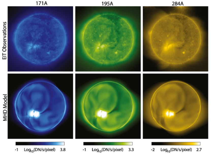
Figure 9: Synoptic maps of the coronal EUV emission at (a) 171 Å, (b) 195 Å and (c) 284 Å for Carrington rotation 1913 (covering the period August 22 to September 18, 1996 at zero longitude), recorded by SOHO/EIT. A large CH (seen dark with respect to the quiet-Sun emission) extends from the north pole into the southern hemisphere. Synthetic (d) 171 Å, (e) 195 Å and (f) 284 Å spectroheliograms, computed from the densities and temperatures obtained with a global MHD model are shown below. Importantly, the overall brightness of the images compares. In addition, several features, including the cross-equatorial extension of the northern polar CH and the the position of the AR south of the equator are well recovered. (Adapted from Figure 6 of Riley et al. (2011). With kind permission from Springer Science and Business Media.)

3.2 Cross-equatorial fields

Global observations often show loop structures extending across the solar equator, thereby connecting the two hemispheres of the Sun (“trans-equatorial loops”; TELs). These are systems of magnetic field lines bridging the solar equator that connect active and/or quiet-Sun regions. The TELs become sheared above the solar surface due to their line-tied footpoints being subject to differential rotation (in the long term), or vortex motions and/or the rotation of sunspots (on shorter time scales). This may also cause the constituent field lines of the TELs to become twisted around a common axis (Bao et al., 2002), which may then be observed in the form of a sigmoid in coronal images. Consequently, an observed sigmoidal structure does not necessarily imply that the underlying non-potential field geometry was already present when the fields emerged (Pevtsov et al., 1997).

3.2.1 Creation of transequatorial loops

The creation of TELs is still far from being understood, mainly because the most frequently employed 2D dynamo models cannot account for their intrinsic 3D nature and formation process (Jiang et al., 2007). 3D models aspiring to resolve the problem are still in their infancy (see Yeates and Muñoz-Jaramillo, 2013; Miesch and Dikpati, 2014, for recent applications).

Active-region magnetic fields that connect across the solar equator and form sigmoidal loop systems have been described by, Svestka et al. (1977) and Tsuneta (1996). They observed newly created loops, connecting across the Sun’s equator in Yohkoh/SXT images and thus that the number of such newly brightened connections increased with time. Yokoyama and Masuda (2010) addressed the question how TELs, appearing bright in Yohkoh/SXT images, can connect very distant regions on the solar surface. In their picture, a series of reconnection processes between equator-bridging weak magnetic fields and their neighbouring strong active-region fields reconfigures the magnetic connectivity such that strong equator-bridging fields develop. Besides, they pictured how this process may result in simultaneous chromospheric evaporation signatures at both footpoints of the TEL system (which had been reported by observationally by Harra et al., 2003). Liu et al. (2010, 2011a) analysed a coronal current sheet which appeared bright in SOHO/EIT 195 Å images above a cusp-shaped flaring loop that connected locations on either side of the solar equator. They presented the first comprehensive set of observations, providing support for the standard picture of flare/CME events (usually referred to as the “CHSKP model” Carmichael, 1964; Hirayama, 1974; Sturrock, 1996; Kopp and Pneuman, 1976, and see also section 4.3). These included the convergence in the legs of the TEL system in the area where the formation of a cusp-shaped flare loop was formed later on, co-temporal radio signatures, as well as an expanding post-flare arcade and coronal dimming in the atmosphere above it.

3.2.2 Properties of transequatorial loops

More frequently global NLFF modelling techniques are being used to investigate the magnetic connectivity between ARs located on either side of the solar equator (see Figure 10). For instance, Tadesse et al. (2014) found that TELs carry only weak electric currents. The departure from a potential state, however, stresses the importance of using magnetic field models that allow departures from a current-free state. At the same time, global force-free magnetic field modelling can strongly depend on the boundary conditions supplied. Measurement errors are particularly high in the transverse component of weak quiet-Sun fields. Photospheric vector field measurements with different instrumentation can differ from each other and influence the corresponding coronal field models. Tadesse et al. (2013) performed a comparison of global NLFF models based on full disk vector magnetograms from SOLIS/VSM and SDO/HMI. In this work some of the TELs clearly observed in coronal images where reproduced with the help of NLFF modelling based on SOLIS/VSM data, but not from the modelling based on SDO/HMI data.

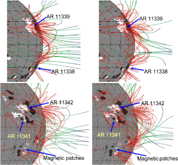
Figure 10: Model magnetic field configurations connecting strong magnetic fields on either side of the solar equator. Selected field lines are calculated from a global (a) potential field and (b) a NLFFF model connecting AR 11339 and AR 11338. Potential and NLFFF model field lines connecting two ARs (11342 and 11341) to strong magnetic patches are shown in (c) and (d), respectively. Red and green line colors indicate closed and open magnetic field lines, respectively. The gray-scale background reflects the measured radial SDO/HMI magnetic field. It can be seen that the non-potential TELs deviate only little from a potential configuration. (Adapted from Figure 5 of Tadesse et al. 2014. With kind permission from Springer Science and Business Media.)

Pevtsov (2000) tested the importance of the chirality (handedness) of active-region magnetic fields for the formation of TEL systems. The results suggested that in roughly two thirds of the cases the connected active-region fields were of the same handedness. Recently, Chen et al. (2010) examined the twist of a larger number of TELs (a subset of the samples analysed by Chen et al. (2006)). They found that the ones that linked ARs displayed an obvious sigmoidal shape and were related to a flaring activity stronger than C-class (i. e., peak SXR fluxes of ${>}10^{6}$ W m^-2). They calculated the ratio $\tilde{L}/D$, where $\tilde{L}$ is the apparent length of the TEL system and $D$ is the apparent distance between the locations where the TEL system seems rooted at the solar surface. $\tilde{L}$ was measured by tracing the length of the coronal loops at the outer edges of the sigmoidal loop system, where they are well distinguished from the faint emission from the (quiet-Sun) background. Higher values of that ratio $\tilde{L}/D$ indicate a more pronounced sigmoidal shape and thus imply a stronger twisting of the associated field lines. They found that most of the TELs possess only weak sigmoidal shapes, indicating a low degree of non-potentiality. It appears that flares above C-class preferentially originate from structures of a specific amount of twist ($\tilde{L}/D\approx 1.4$). It is an important future task to model the associated cross-equatorial 3D coronal magnetic field and its evolution with the help of global force-free and time-dependent MHD models in order to reveal the importance for eruptions to occur (see also section 4.4).

3.3 Spatio-temporal aspects of activity

3.3.1 Cyclic changes of the coronal magnetic field

As the coronal field responds to photospheric changes, it also changes on global scales with an approximately decade-long periodicity. Bright loop systems appear at higher latitudes ($\gtrsim 30^{\circ}$) at the beginning of a solar cycle and the activity belts progressively move closer to the equator as the cycle progresses.

Coronal holes vary in shape and position with the solar cycle as well (see review by Cranmer, 2009, and section 6). While polar CHs, if present at all, are found to cover only small areas around the poles during solar maximum, they tend to reach their largest extents around solar minimum and then occasionally extend to latitudes as low as $\approx 60^{\circ}$. Low-latitude CHs emerge preferentially around solar maximum and near the activity belts due to the occasional accumulation of unipolar flux during the emergence of ARs. If a sufficient amount of unipolar flux emerges and clusters together to form extended patches, the associated fields may be open. As a consequence, the open flux on global scales varies in the course of the solar cycle (its long-term variation was computed by Solanki et al., 2000, 2002; Schrijver et al., 2002; Jiang et al., 2011). Since the interplanetary magnetic field is fed by the magnetically open regions on the Sun, a similar modulation over the course of a solar cycle was expected too. Thus, it was surprising that the magnitude of the radial interplanetary magnetic field strength does not show a strong dependence on the activity level. Wang et al. (2000b) and Wang et al. (2000a) investigated why this is so and argued that the reduced area occupied by open fields around solar maximum is compensated by their, on average, higher field strengths. As a consequence, the open solar flux is nearly maintained throughout the solar cycle.

During solar activity maximum strongly emitting (bright) loop systems occupy a considerably larger volume within the corona. Associated active features, including flares (Bai, 2003; Zhang et al., 2011) and coronal streamers (Li, 2011) as well as super-ARs (i. e., ARs associated to repeated flaring and mass ejections, cf., Tian et al., 2002) were found to be distributed inhomogeneously in solar longitude. They seemingly relate to “active nests” or “active longitudes”, which had originally been postulated based on similar trends seen in surface magnetic field observations. Chidambara Aiyar (1932), for instance, found sunspots to preferentially emerge at particular longitudes on the solar disk, which has been almost immediately attributed to projection effects and/or selection criteria by Carroll (1933). Follow-up studies concerning the preferred locations (longitudes) of sunspot formation delivered inconsistent and partly contradictory results. Even today, the possible number, migration, life-times, long-term behaviour and the particular method to track them remains a subject of debate (see Berdyugina and Usoskin, 2003; Usoskin et al., 2005; Pelt et al., 2006; Usoskin et al., 2007; Weber et al., 2013; Gyenge et al., 2014).

3.3.2 Association to dynamic events

Mass ejecta cause severe changes of the coronal magnetic field, leaving it behind in a massively reconfigured configuration. Changes in the coronal magnetic field configuration, owing to magnetic reconnection of non-potential closed magnetic fields below coronal streamers, for example, are in fact thought to be the building blocks of the basic mechanism of coronal mass ejecta (for reviews see Forbes, 2000; Chen, 2011). Liu et al. (2009b), for instance, presented observations of short-lived as well as of lasting deformations in association with an observed CME. The transient modifications were seen in the form of structures, neighbouring the ejection site, pushed aside and bouncing back. Lasting distortions were observed in the form of displacements of the associated helmet streamer and the shrinkage of coronal holes (see Figure 11).

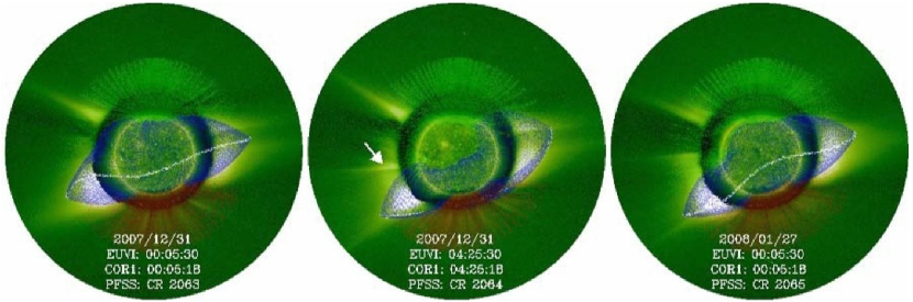
Figure 11: Composite STEREO/SECCHI EUVI 195 Å (Sun at the center of each image) and COR1 (surrounding disk) images (a) before, (b) immediately after and (c) 27 days after a CME. The white arrow in (b) indicates a streamer-like structure behind the CME which was interpreted as the current sheet in its wake, also because it did not exist before (compare (a)), nor about a month after the ejection (compare with (c)). The blue lines represent magnetic field lines calculated from a global PFSS model and projected onto the STEREO/SECCHI images. In a similar manner, the white line displays the source surface neutral line. It can be seen that, as a consequence of the CME, the coronal streamer migrated southwards (compare the position of the coronal streamer above the south-east limb of the Sun in (a) and (b)) but survived and persisted for more than one additional solar rotation (note the location of the streamer in (c)). (Figure 3 of Liu et al. (2009b). © AAS. Reproduced with permission.)

On the other hand, it has also been reported that, in a considerable number of cases, the coronal environment barely responded to or appeared insensitive to the occurance of mass ejections. This viewpoint has been championed by Sime (1989), who argued that the global evolution of the coronal magnetic field gives rise to CMEs but is not really influenced by them. In other words, the ejecta may be associated to the streamer belt but may not have a lasting effect on it. This was supported by the observation that the streamer belt appeared to reestablish itself within a few days after ejections (Zhao and Hoeksema, 1996). Although, it is certain that CMEs are associated with the belt of coronal streamers (Hundhausen, 1993), the disruption (or disappearance) of an associated streamer was observed in only $\approx 15\%$ of the cases observed (Subramanian et al., 1999; Floyd et al., 2014). In summary, whether mass ejections are only a response to or a contributing factor to the coronal restructuring is not yet clear (Liu et al., 2009b).

It is generally agreed, however, that only mass ejections (which inevitably drag the embedded magnetic field along) are capable of physically reducing the coronal magnetic helicity, which is tightly related to the structural properties of the magnetic field (Moffatt, 1969). We discuss this in the following.

3.4 Magnetic helicity budget

3.4.1 Helicity dissipation and helicity transport

Magnetic helicity is dissipated on significantly longer scales than the magnetic field and consequently the dissipation time in the corona is too long to relevantly reduce the helicity (Berger, 1984). For the helicity budget of ARs and quiet-Sun regions see sections 4.6 and 5.2.6, respectively. Since magnetic helicity cannot be efficiently dissipated, it is approximately conserved in the absence of ejecta, i. e. the magnetic helicity in the solar corona will continuously build up. That has important consequences for the magnetic field relaxation towards a lower energy state. It implies that in the course of a flare, but lacking a mass expulsion, a non-potential field can only relax to another, lower-energy configuration of the same helicity content (i. e., a constant-$\alpha$ field; see Taylor, 1974; Heyvaerts and Priest, 1984; Taylor, 1986). However, the coronal magnetic field may never entirely relax to this constant-$\alpha$ (conserved-helicity) state, because the required “complete” reconnection is not expected to occur due to the line-tying of the coronal magnetic field structures at photospheric levels. This also inhibits the simultaneous formation of numerous current-sheets (see Antiochos and DeVore, 1999, and references therein).

The majority of ejecta, including CMEs associated with disappearing filaments (Yurchyshyn et al., 2001; Cho et al., 2013) or eruptive X-ray loops (Mandrini et al., 2005; Zheng et al., 2011), propagate away from the Sun in the form of magnetic clouds (MCs) and hence actively carry helicity away. MCs are force-free regions of enhanced magnetic field strength, with the field vector monotonically rotating as they journey with the solar wind. There are the moving large-scale helical structures described by Burlaga et al. (1981); Burlaga (1988). They are a sub-set of interplanetary CMEs that consist of plasma and magnetic field, expanding behind a shock wave into interplanetary space. Gopalswamy et al. (1998) suggested that MCs originate from the structure overlying an eruptive prominence and its associated CME and include the coronal cavity and a bright frontal structure. A typical MC may carry a magnetic helicity of some $10^{41}$ Mx² to $10^{43}$ Mx² (Cho et al., 2013). This, and considerations based on surface magnetic field measurements, permit to estimate the amount of helicity transported away on a global scale during one solar cycle as $\approx 10^{45}$ Mx² to $10^{46}$ Mx² (Bieber and Rust, 1995; Rust, 1997; DeVore, 2000; Berger and Ruzmaikin, 2000; Georgoulis et al., 2009; Zhang and Yang, 2013).

3.4.2 Hemispheric trends

When estimating the global helicity budget, it is of importance to take the Sun’s differential rotation into account. DeVore (2000) estimated the effect which the Sun’s differential rotation has on the shearing of an active-region magnetic field. He estimated an accumulated helicity as $\approx 10^{43}$ Mx² during a characteristic active-region lifetime of $\approx 120$ days. However, the differential rotation cannot represent the only source of helicity supply to the corona Démoulin et al. (2002). Georgoulis et al. (2009) suspected that the contribution of differential rotation to the total amount of injected magnetic helicity amounts only to about 20%. The dominant source of injection, they argued, must be due to the plasma flows within ARs (see section 4.6.1). This agrees with earlier results which stated that the amount of helicity injected by differential rotation in ARs may comprise roughly 10% to 50% of that injected by motions within the ARs themselves (Démoulin and Pariat, 2009, and references therein).

The injection of magnetic helicity does not appear to display any periodicity, indicating it to be a rather unforeseeable process (Georgoulis et al., 2009). Although temporal periodic patterns have not been found, some systematics regarding the spatial distribution of helical features on a global scale are known. Several observational features indicating the handedness of structures, such as sunspot whorls (Hale, 1925; Richardson, 1941), chirality of filaments (Rust, 1967; Pevtsov and Balasubramaniam, 2003; Bernasconi et al., 2005) and S-shaped coronal X-ray brightening (Rust and Kumar, 1996; Canfield et al., 1999) revealed a dominant positive helicity pattern in the northern solar hemisphere and a dominant negative one south of the solar equator. The associated magnetic fields in the northern and southern hemisphere are dominated by right- and left-handedness, respectively (Seehafer, 1990; Pevtsov et al., 1995). Interestingly, these patterns do not change from one activity cycle to the next.

This tendency, however, was found to be less pronounced for active-region filaments than for filaments in the QS Pevtsov and Balasubramaniam (2003). Bao et al. (2002) gave a hint why there is a weaker hemispheric trend of active-region magnetic fields. They argued that the chirality introduced by the same mechanism acting on a rising flux tube throughout the convection zone, or acting on the flux tube after emergence through the photosphere may be opposite. The dominant contribution would then determine the chirality of an AR which would not necessarily follow the hemispheric trend. Using a magneto-frictional model, Yeates et al. (2008) were able to reproduce the skew of more than 90% of considered filaments (observed in H$\alpha$ images) correctly, even including exceptions from the hemispheric trend. Yeates and Mackay (2012) recently presented the first long-term simulation of the chirality of high-latitude filaments and were able to recover the hemispheric trend. According to them, the apparent handedness depends on which of the two effects, creation of helicity by differential rotation or its transport from active latitudes, is stronger. They found that the latter is generally stronger, except during the early years of a solar cycle. Further evidence for the dependence of the chirality of features in the solar atmosphere on the phase of the solar cycle comes from SXR loops (Zhang et al., 2010b) and active-region magnetic fields (Zhang et al., 2010a).

Having started on magnetic fields on active-region scales, we continue to discuss their magnetic and helicity properties in the next section.

4 Coronal active-region magnetic fields

4.1 Coronal loops

The frozen-in condition for the coronal plasma and magnetic field is valid in most of the coronal environment. The sole exceptions are the small diffusion regions in strong current concentrations, the so-called “current sheets” (see section 4.2). Much of the plasma in the corona is confined by the magnetic field in the form of thin closed flux tubes. The loop plasma may be heated by a number of possible mechanisms (for a review see Reale, 2010). As a consequence, pressure and density of the gas within the magnetic loops are enhanced compared to the values reached by the surrounding gas and the coronal loops appear bright in coronal radiation. This property is of great advantage for the investigation of the dynamics in the corona: the bright structures serve as an indirect tracer of the coronal magnetic field.

Owing to its high temperature the coronal plasma emits radiation predominantly at X-ray, EUV and radio wavelengths. The bulk of the coronal loops hosts plasma of temperatures of $\approx$ $10^{5}$ K to $\approx$ 10 MK. The lower and upper limits are representative of cool and flaring loops, respectively (Reale, 2010). Coronal loops often fan out from relatively compact footpoints at the solar surface, arranging themselves in dome-like structures with multiple layers. The individual loops are thought to have a very narrow distribution of temperatures within the loops themselves – neglecting their footpoints – though the loops within an AR may have very different temperatures (Del Zanna and Mason, 2003; Aschwanden and Boerner, 2011). In the corona, where the field fans out with height, thin constituent strands are discernible. At present, several spectral EUV channels are used to observe and study coronal loop fine structures since they appear well defined around the wavelengths 171 Å and 193 Å. At the highest spatial resolution presently achievable, in the form of Hi-C data, the density and temperature structure across the observed thin strands varies on a spatial scale of roughly $0\mbox{$.\!\!^{\prime\prime}$}1$; alternatively, one may state that a diameter of $0\mbox{$.\!\!^{\prime\prime}$}1$ represents an upper limit for the strands which make up an observed loop (Cirtain et al., 2013; Peter et al., 2013).

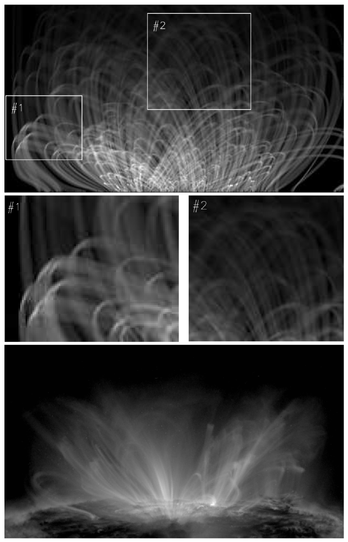
Figure 12: (a) Coronal emission simulated from flux tubes (calculated from a potential magnetic field model) filled with hydrostatic, isothermal plasma. The gray-scale reflects the squared column emission in arbitrary units. Rectangular areas labeled as #1 and #2 highlight areas where loops do not notably expand with respect to their neighbours and where loops turn towards the observer, respectively. Close-ups of these regions are shown in panels (b) and (c), respectively. (d) EUV emission from active-region loops as seen above the solar limb in an SDO/AIA 171 Å image. The numerically synthesized brightness variations are well visible in the observed corona: the emission of loops with less varying apparent cross section is enhanced (compare panel (b)) and horizontally elongated where loops turn towards the LOS (compare panel (c)). (Adapted from Figures 17 and 18 of Malanushenko and Schrijver (2013). © AAS. Reproduced with permission.)

It has long been puzzling why especially the loops seen in coronal images do not show a significant variation of their width with height in the atmosphere. Given magnetic flux tubes expand with height in the solar atmosphere, one would naturally expect this to be reflected in form of a clear height-dependence of the emission observed from the thin threads which compose the flux tubes (DeForest, 2007). Instead, an apparently constant cross section and more or less constant brightness along the loops, but no significant expansion was observed at the two wavelengths mentioned above. This is the result of the analysis of coronal loops seen in Yohkoh/SXT images (Klimchuk et al., 1992), and EUV observations with TRACE (DeForest, 2007) as well as with SDO/AIA (Aschwanden and Boerner, 2011). It has been argued that this might just reflect the fact that the coronal loops are entities of a constant diameter (Klimchuk, 2000), although force-free magnetic field models do not support such an interpretation.

Physical reasons for the geometric distribution of the observed coronal loop emission is now beginning to come from numerical experiments. Peter and Bingert (2012) used an MHD model to investigate the temporal evolution of the corresponding synthesized coronal emission. They were able to show how emission of seemingly constant width may arise from an expanding flux tube. They argued that the plasma indeed fills the fanning-out magnetic field structure, but that it does not equally contribute to the emission perpendicular to the plasma loops’ axis. The radiation from the plasma at the outer edges, i. e., the “envelope” of the expanding magnetic field is emitted from plasma at a lower temperature. Consequently, this radiation is missed in images showing the bulk of the emission at, say, 171 Å and resulting in coronal images showing loops of nearly constant cross section. Peter and Bingert (2012) also pointed out that the appearance of the coronal loops may even be caused by the specific perspective at which the coronal loops are seen (see also Mok et al., 2008). Similar results have been found recently by Malanushenko and Schrijver (2013), who investigated a large sample of flux tubes that were based on a potential field model. They were able to assign well known observed features to both, projection effects as well as the deviation of the flux tubes’ cross section from a circle along its length. These include the enhanced brightness of loops which seemingly do not expand much in the plane of sky, compared to neighbouring loops which seem to do so, and the characteristic elongated bright emission where loops turn towards the LOS (see Figure 12).

4.2 Local field topology

The bright coronal loops within ARs connect photospheric locations of enhanced magnetic flux of opposite polarity. On a global scale, as discussed in section 3, such loops are observed only within certain latitude bands, the activity belts. The active-region fields are often composed of strong sunspot fields surrounded by plage regions of weaker field strengths. Prominent ensembles of active-region loops preferentially connect locations of strong magnetic flux inside an AR (i. e., sunspots and/or plage regions), or they have one footpoint located in an AR and the other in the enhanced flux of the surrounding network (Schrijver et al., 1999).

4.2.1 Magnetic skeleton

The building blocks of the coronal magnetic field include the locations of a vanishing magnetic field (“null points”), field lines which separate topologically distinct regions of space (forming “separatrix surfaces”), as well as special field lines at the intersection of such surfaces which connect two null points (“separators”). The sum of all these special locations, field lines and surfaces is called the “magnetic skeleton” (see Longcope, 2005; Priest, 2007, and Figure 13). Separatrix surfaces and separators are places where the magnetic field is discontinuous, i. e., the field lines with footpoints on either side connect to rather different positions on the Sun. Consider, for instance, a field line which originates from the vicinity of the positive polarity $P$ (indicated by the red, dashed-dotted lines) in Figure 13. If the positive-polarity footpoint of the field line is located within the separatrix surface associated to $P$ (black dashed dome), the field line can only close down in the vicinity of the neighbouring negative polarity $n$. If the footpoint, however, is shifted to a location just outside of the associated separatrix surface, the field line can no longer connect to $n$, because field lines do not cross separatrix surfaces or separators. Instead, it may connect to another neighbouring negative polarity $N$ by running all along outside of the separatrix surfaces associated to $P$ and $N$ (red dash-dotted dome).

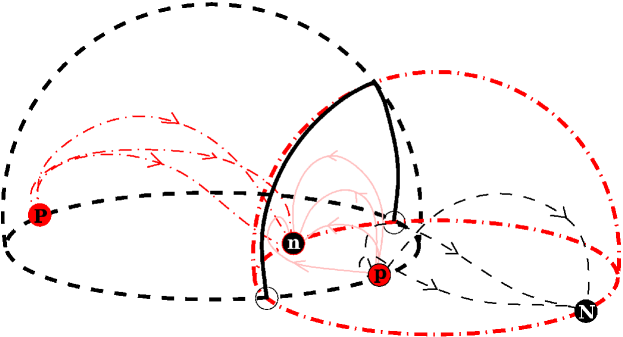
Figure 13: Sketch of a 3D magnetic skeleton. Circles with red and black filling represent magnetic sources ($P$, $p$) and sinks ($N$, $n$), respectively, i. e., positive and negative flux concentrations. Black (dashed) and red (dash-dotted) curves represent sample field lines which close within the domain bounded by the positive and negative separatrix surfaces (thick red dash-dotted and thick black dashed outlined domes, respectively). The separator field line (black solid curve) runs where the positive and negative separatrix surfaces intersect, connecting two null points (black circles). It also marks the intersection of at least four distinct flux domains. Pink solid curves represent field lines that connect $p$ and $n$, which must close below the separator. Note that $P$ and $N$ can only be connected by field lines running outside of both separatrix surfaces, i. e.  they have to bridge the separator. (Adapted from Priest and Forbes (2002).)

4.2.2 Association to current-sheets and magnetic reconnection

When a magnetic configuration evolves quasi-statically or dynamically, different flux domains develop as pictured above. It is possible to trace the different magnetic flux domains in the corona and their footprint on the solar surface, given that the 3D magnetic field configuration is known (Priest and Démoulin, 1995; Demoulin et al., 1997; Démoulin, 2006; Titov et al., 2002). One can determine the position of the conjugate-polarity footpoint of a certain field line. Applying a horizontal shift to the location of the footpoint from which the field line calculation is started, the places of strongest variations regarding the location of the opposite-polarity footpoint are detected, indicating the location of “quasi-separatrix layers” (QSLs; Priest and Démoulin, 1995; Demoulin et al., 1997; Titov et al., 2002). There, the magnetic connectivity is not discontinuous but has steep gradients. This leads to the formation of current sheets (Titov, 2007) in which electric currents may be efficiently dissipated (Aulanier et al., 2005; Bellan, 2006; Pariat et al., 2009). Note that this implies that current sheets preferentially form where QSLs border each other (Schrijver et al., 2010).

Current sheets are regions in space where the magnetic field strength, and thus the magnetic energy density, is locally enhanced. In the collisionless environment of the solar corona, current sheets are transient features which diffuse away but, as long as they exist, they have important consequences for the field and plasma they contain. Most importantly, the resistivity within a current sheet is locally enhanced and as a consequence, unlike in the coronal surroundings of the current sheet, the plasma is – in contrary to the surrounding corona – not frozen into the field. Thus, they are favourable locations for changes of the magnetic topology to happen, i. e., where the magnetic field may change direction and/or magnitude (see chapter 2 in Priest (1982), Priest and Forbes (2007), chapter 6 in Priest (2014), and also section 4.5.3).

As pointed out by Parnell et al. (2008), knowledge about the magnetic skeleton is necessary if one aims to determine the location, type, rate and frequency of reconnection events. Therefore, the magnetic skeleton has been investigated for complex magnetic field configurations also with the help of MHD experiments satisfying solar-like parameters. Maclean et al. (2009) performed MHD simulations, using a potential field based on SOHO/MDI observations as an initial equilibrium. They investigated the evolution of the magnetic field around an EUV bright point observed in TRACE 171 Å images. They simulated the effect of the observed rotation of one of the main photospheric magnetic sources of a bright point. They could also show that the resulting build-up of electric currents may have enabled magnetic reconnection at the separatrix surfaces associated with the rotated magnetic source. They commented that more research must be undertaken in order to determine which parts of the separatrix surfaces host strong electric currents. This was partly addressed by Parnell et al. (2010), who studied the magnetic skeleton in the course of magnetic flux emergence into a pre-existing magnetic field. Their results indicated that locations along separators are favourable locations for magnetic reconnection to occur.

4.2.3 Relation to dynamic phenomena

Because the trigger for magnetic reconnection has often been suspected around an existing coronal null point or within a QSL, studies have been undertaken to relate flare-associated features to the magnetic topology of the corona (Luoni et al., 2007; Baker et al., 2009; van Driel-Gesztelyi et al., 2012; Sun et al., 2012a). Aulanier et al. (2000) inferred the location of a coronal null point and separatrix surfaces from a potential field reconstruction and highlighted that, a current-free model cannot be expected to reproduce the observations in detail – especially in the presence of strong shear. Nevertheless, it can be expected that it should be capable of recovering the basic, underlying coronal magnetic field topology. A similar finding was presented by Su et al. (2009), who employed, besides a potential field model, also a NLFF field model with an artificially inserted flux rope, forced to emerge into the force-free model corona. Their work revealed a line of coronal null points not only in the NLFF but also in the potential field representation. This supported the idea that a potential field model may indeed be sufficient to gain information on the basic coronal magnetic field topology. A less supportive conclusion was reached by Sun et al. (2012a), who found that the number and location of coronal null points were not the same for NLFF and current-free field models. Specifically, the position of a coronal null, as inferred from an NLFF field solution was clearly displaced from the location calculated from the associated potential field model. This mismatch, they argued, might have been caused by the high non-potentiality of the investigated active-region field which made the current-free model fail to realistically account for its structure.

Aulanier et al. (2000) and Su et al. (2009) found the shape of observed flare ribbons to be closely associated to the intersection of separatrix surfaces with the lower atmosphere. The spatial proximity between flare ribbons and QSLs agrees with the picture of confined flares (for reviews see Priest and Forbes, 2002; Shibata and Magara, 2011), which relates flare ribbon emissions to particles that are accelerated at the coronal reconnection site and that follow the separatrix field lines downward. Eventually encountering the denser layers of the lower atmosphere, they lose their energy due to collisions, but increase the radiation emitted at these locations by heating the surrounding plasma. Also using a potential field model, Masson et al. (2009) explained the flare ribbons observed in association with a small flare by the photospheric intersections of field lines that passed the vicinity of a coronal null point (similar to what was found by Chandra et al., 2009, see Figure 14). They found that these field lines formed a surface which enclosed the flux domain of a “parasitic polarity” (that is a patch of a certain magnetic polarity surrounded by fields of opposite polarity) and that the geometry agreed closely with the theory of confined flares.

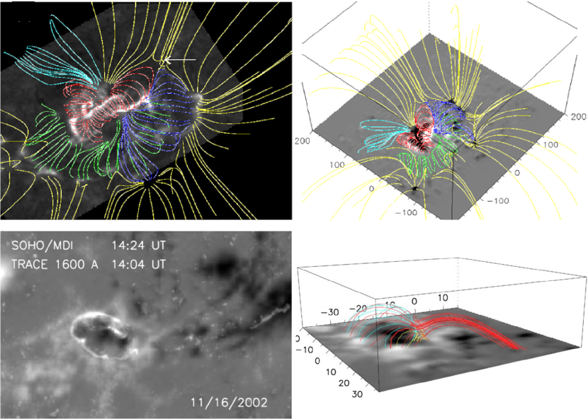
Figure 14: (a) Magnetic topology of AR 10365 on 27 May 2003, estimated from a current-free field model. The white arrow in (a) indicates the possible location of a coronal null point, based on the associated current-free field configuration. Selected field lines that outline the basic magnetic field configuration are displayed on top of a near-in-time H$\alpha$ image taken at the Solar Observatory Tower Meudon. Strongest emission in (a) outlines the location of flare ribbons (that is, where newly reconnected field lines are line-tied to the low atmosphere). (b) The same model configuration, shown on top of the SOHO/MDI LOS magnetogram (gray-scale, where positive/negative polarity corresponds to white/black areas). Sample magnetic field lines, connecting the AR and its periphery are shown in yellow. Green, light and dark blue, as well as red field lines connect the observed flare ribbons to other regions within the AR. (Adapted from Figure 8 of Chandra et al. (2009). With kind permission from Springer Science and Business Media.) (c) TRACE 1600 Å emission (bright ribbon and kernels) associated to a C-class flare on November 11, 2002, overlaid on a SOHO/MDI photospheric LOS magnetic field (gray-scale background; white/black represents positive/negative polarity) of AR 10191. (d) Sample field lines outlining the potential field reconstruction of the associated coronal field. The red, yellow and blue lines indicate a coronal null-point topology. (Adapted from Figures 2 and 3 of Masson et al. (2009). © AAS. Reproduced with permission.)

Note that magnetic field lines are fictitious constructs, meant to outline the direction of forcing by the magnetic field. Thus, they are often related to physical coronal structures, since charged particles in the corona feel the force exerted by the magnetic field (Lorentz force). As a consequence, for instance, heat conduction is most efficient along the magnetic field. Similarly, density enhancements and small localized disturbances propagate along field lines, and plasma flows are mechanically confined by the field (Longcope, 2005). Such flows persist on time scales similar to that of the slow quasi-static evolution of the magnetic field, i. e., of the order of hours, and have indeed been found near QSLs. Early on, Marsch et al. (2004) were able to show the quasi-static nature of active-region flows and their close connection to the coronal magnetic field structure. Using a LFF field model, they were able to associate sharp changes in the Doppler velocity (inferred from SOHO/SUMER Dopplergrams) to the border between topologically different field configurations (open and closed). Furthermore, there seems to be a connection between the strength of the flows and the underlying magnetic field: the strongest flows seem to be associated to that portion of QSLs which are situated above strong magnetic fields (Baker et al., 2009).

4.3 Temporal evolution of active-region magnetic fields

The active-region corona that spans from the coronal base until about 100 Mm above the solar surface, is a low-$\beta$ environment (see Gary, 2001, and section 1.2.3). That implies that the evolution of the magnetic field dictates the mass, momentum and energy flow. This is because the dynamic pressure exerted by the solar wind within the Alfvén radius, i. e., the range within which any escaping material is forced to rotate rigidly with the Sun, is small compared to the magnetic pressure, the latter also well exceeding the gas pressure there (see chapter 9 in Stix (2002)). The shuffling around of magnetic field lines at photospheric levels by the convective motions at (sub-)photospheric levels determines the temporal evolution of the coronal field above. Thanks to the high Alfvén velocity ($\approx 10^{3}$ km s^-1), the coronal plasma can quasi-statically adjust to the driving (sub-)surface convective motions (with characteristic speeds of a few km s^-1; see chapter 6 in Stix, 2002). This, together with the underlying field topology determines the fate of coronal active-region magnetic fields. In most cases the evolution of the corona is a slow transition between neighbouring equilibrium states.

A slow, quasi-static evolution means that the coronal magnetic fields adjust to the random or systematic motion of their line-tied photospheric footpoints without a sudden energy release, i. e., without a major eruption. Note that the condition of the magnetic field being frozen in the plasma and its more or less passive advection by photospheric flows is referred to as line-tying (see Longcope, 2005). That does, however, not preclude the presence of dynamic phenomena. For instance, at the edges of ARs, outflows have often been observed with velocities of tens of km s^-1. This has actually been proposed to be important for the solar wind Brekke et al. (1997); Winebarger et al. (2001); Sakao et al. (2007). Such flows might arise from the reconnection between small-scale emerging fields and larger-scale open field lines of ARs (Liu and Su, 2014). Also SXR jets are sometimes observed at the boundaries of ARs (Shimizu et al., 1994), often associated with parasitic polarities (Schmieder et al., 2013). But despite such small-scale events, for most of the time, the magnetic field of an AR evolves slowly and can be considered to be in equilibrium. At typical coronal conditions, the magnetic energy density – which is a measure for the magnitude of the associated pressure – is at least three orders of magnitude larger than the gravitational, thermal or kinetic energy density (Forbes, 2000). Under equilibrium conditions, this implies that the Lorentz force vanishes and that the field can be considered to be force-free (see section 2.2). Once equilibrium is lost, however, this might no longer be true and dynamic forces come into play that compensate the non-vanishing magnetic forces.

4.3.1 Dynamic evolution: eruptive phenomena

Forced away from its equilibrium position, or, more precisely, from a quasi-static oscillation around its equilibrium position, a configuration of the coronal field may develop in two ways. Either it reaches a metastable state or a non-equilibrium state (Priest and Forbes, 2002). A metastable configuration is stable with respect to small perturbations because it involves a stabilizing element. A corresponding coronal configuration would be in the form of, e. g., a twisted flux rope bridged by a loop arcade, where the latter holds the configuration steady (Sturrock et al., 2001). A non-equilibrium state, on the other hand, is instable against any further perturbation and its evolution is then determined by the evolutionary path of that initially small perturbation. We are facing different types of evolution, in the form of a growth of the perturbation, an oscillation, or eventually a damping out. Given the appropriate trigger, a meta- or non-stable state may evolve further to a state where mass and/or energy is released due to an associated change of the field topology. Examples of force-free equilibria with stable and instable configurations (dependent on model parameters) have been constructed by Titov and Démoulin (1999). Instable configurations have been investigated with numerical MHD simulations by Török and Kliem (2005). Importantly, the morphology and dynamic evolution of a modelled erupting flux rope (an eruption triggered by an ideal kink instability) was found to be in agreement with an observed eruptive flare.

Associate releases of mass and/or energy are called flares, eruptive prominences and CMEs, depending on the emission and dynamics observed (for reviews see, Benz, 2008; Fletcher et al., 2011; Mackay et al., 2010; Parenti, 2014; Hudson et al., 2006; Webb and Howard, 2012). Flares involve sudden enhancements of electromagnetic radiation, caused by accelerated particles and excessive heating of the coronal plasma. During an eruptive prominence the material initially trapped inside is partially or completely expelled from the Sun. CMEs involve the expulsion of huge masses of coronal plasma into interplanetary space, spanning the range of roughly $\approx$ $10^{12}$ kg to $\approx$ $10^{16}$ kg (see Vourlidas et al., 2010, 2011, for a comprehensive analysis of CME masses during a full solar cycle). Many attempts have been made to develop models to describe the features associated with a loss of equilibrium, including the pre-eruptive coronal magnetic field structure, the triggering mechanism and the temporal evolution of the eruption itself. It is outside the scope of this review to summarize all existing models of eruptive processes in the solar atmosphere. Instead, we refer here to the comprehensive reviews on flare (Forbes et al., 2006; Chen, 2011) and CME models (Forbes, 2000; Shibata and Magara, 2011).

4.4 Favourable conditions for eruptions

To find the conditions under which the magnetic field of a (part of an) ARs is likely to erupt, one has to analyse the corona as well as the underlying parts of the atmosphere before an eruption occurs (for reviews see Schrijver, 2009; Chen, 2011). Favourable conditions for eruptions include strongly twisted or sheared magnetic structures embedded in a less-sheared magnetic system (Hao et al., 2012), the rapid emergence/evolution of strong magnetic flux concentrations (Wang et al., 2004a; Sun et al., 2012b), and/or a complex magnetic field topology (Sun et al., 2012a).

4.4.1 Magnetic flux emergence and complex magnetic field structure

A complex magnetic field structure may include parasitic polarities, highly sheared fields, strong gradients and long PILs, not necessarily all at the same time or in the same event (van Driel-Gesztelyi and Culhane, 2009). For magnetically complex ARs a tendency to be more CME-productive has indeed been found (Chen et al., 2011). Large flares mainly originate from ARs with a complex photospheric magnetic field configuration, the largest ones from $\delta$-configurations (see review by Benz, 2008, and references therein). Note that a $\delta$-configuration denotes umbrae of opposite polarity existing within a single penumbra. Only rarely are spotless regions reported to be the source of major flares (Ruzdjak et al., 1989; Sersen and Valnicek, 1993; Li et al., 1995). M- and X-class flares are considered to be ”major” flares in this context with SXR peak fluxes on the order of $10^{-5}$ W m^-2 and $10^{-4}$ W m^-2, respectively. Ruzdjak et al. (1989), however, mentioned an enhanced occurrence rate of a specific type of eruption in spotless regions, namely two-ribbon flares, involving two progressively spreading bands of chromospheric emission.

As noted by Schrijver (2009), an eruption might not be triggered per se due to flux emergence but only if a sufficient amount of magnetic flux emerged. The imbalance of the emerging magnetic flux does not seem to be crucial for an eruption to occur, although it might play a role. Choudhary et al. (2002) noted that only roughly one third of their analysed cases showed a flux asymmetry of more than 10%. A super-AR, however, was found to exhibit a flux imbalance of $\approx 40$% which, they admitted, could have partly been caused by instrumental effects. It is worth noting that, such analyses often suffer the problem of projection effects which is noticeable in the degree of flux imbalance systematically increasing with distance from the disk center (Green et al., 2003). Chen and Wang (2012) recently revisited the importance of flux-imbalance for the eruptive nature of ARs; they only considered ARs that fulfilled certain selection criteria, including being observed within $\pm 30^{\circ}$ from the central meridian and being associated to major flaring activity. They analysed 14 ARs and found a significant imbalance of magnetic flux: more than half of the ARs showed a flux imbalance of $\gtrsim 20$% (see also Tian et al., 2002; Romano and Zuccarello, 2007). However, thermal effects on the photospheric line profiles can influence the determination of magnetic flux. This can lead to a seeming imbalance between the two polarities of an AR if, e. g., one polarity of the AR is composed more of sunspots, while the other polarity has more plage. Consequently, this topic needs further study.

4.4.2 Magnetic shear and twist

An eruption may also be triggered if, owing to the motion of its photospheric footpoints, a coronal loop arcade is sheared too much (Priest and Forbes, 2002). It has long been known that the combination of strong fields and strong shear seem an essential ingredient to, for example, ribbon flares (Hagyard and Rabin, 1986). Strong shear may develop due to sunspot motions, converging giant convection cells, as well as due to the emergence, cancellation and submergence of magnetic flux (see Hagyard et al., 1984a, and references therein; see also Wang 1994). Note, however, that it might not always be possible to judge whether horizontal flows caused the observed shear or if an arcade already emerged as a sheared configuration (Wiegelmann et al., 2005b). Krall et al. (1982) compared the evolution of the transverse magnetic field component to the motions within a flare-productive AR observed in white light. They found that over a period of several days the observed shearing motion resulted in an ever increasing field alignment with the PIL and was associated to the onset and increase of flaring activity, and which has been supported by the MHD model results of Wu et al. (1984). Force-free modelling results have initiated the search for a possible critical amount of shear which, once reached, would inevitably trigger an eruption (Low, 1977a, b), but for which observational support seems sparse.

Hagyard et al. (1984b) estimated the critical shear to lie in the range $80^{\circ}\lesssim\theta\lesssim 85^{\circ}$. They defined the shear angle, $\theta$, as the angular difference between the orientation of the transverse field component and the direction perpendicular with respect to the PIL. Consequently, $\theta=0^{\circ}$ implies a field with no shear and $\theta=90^{\circ}$ would account for a transverse field parallel to the PIL. Sivaraman et al. (1992) followed a different approach: they used H$\alpha$ observations to determine the orientation of the major axis of filaments (as an indication for the direction of the PIL) with respect to an approximation to the orientation of the potential field azimuth. The latter has been defined by the direction perpendicular to a straight connection between the two main spots of the associated bipolar sunspot group. Their study revealed that flares occurred only when the angle between the principal filament direction (i. e., the PIL) and the direction of the potential field azimuth exceeded $\approx$ 85^∘ (using the same notation for the shear angle as above).

Another source of instability is the amount of twist of a coronal structure, as induced by systematic motions of the photospheric footpoints of the field. For instance, an equilibrium coronal loop becomes instable if its length is stretched beyond a critical value, or if it is twisted by photospheric motions (Priest, 1978). For twisted magnetic field configurations, different critical thresholds were found within numerical experiments, including uniformly twisted toroidal or periodic, line-tied cylindrically symmetric configurations (Hood and Priest, 1981; Baty and Heyvaerts, 1996) and locally twisted configurations (Baty and Heyvaerts, 1996; Mikić et al., 1990; Fan and Gibson, 2003; Török and Kliem, 2003). Note, the results of all of these model experiments agree fairly well on the critical amount of twist: the field lines must perform more than one full turn ($T>2\pi$) about the center of the flux tube for it to become kink-unstable, which would be observed as an eruption for under coronal conditions. These numerical considerations also revealed that the critical twist, tends to rise with increasing aspect ratio, that is the ratio of the loop length to its cross-sectional diameter (Einaudi and van Hoven, 1983; Török et al., 2004). On the other hand it is smallest for loops of a strong magnetic field, for given temperature and density values (Priest, 1978).

4.5 Magnetic energy budget

4.5.1 Energy build-up and storage

Magnetic flux continuously emerges from where it is generated through the photospheric layers and punches into the pre-existing coronal magnetic field. At the same time, small- and large-scale convective motions in the photospheric layers, shuffle around bundles of frozen-in magnetic field lines. The energy required to perform the work of moving magnetic structures against the ambient magnetic field contributes to the magnetic energy content of the coronal field (Parker, 1987). The two major contributions to the transport of magnetic energy to the corona are the emergence of material through the photosphere from below, dragging magnetic field along, and horizontal motions of the photospheric material that increase the shear of the magnetic field above (Wang, 1995). The footpoint motions of coronal loops result in an energy flux of $\approx$ $10^{4}$ W m^-2 and $\approx$ $10^{6}$ W m^-2, for typical photospheric quiet-Sun and active-region conditions, respectively, to the corona. This is at least ten times larger than the corresponding radiative and conductive losses in chromosphere and corona (Bellan, 2006; Parnell and De Moortel, 2012).

The random displacements of the line-tied footpoints of the coronal field-lines naturally lead to “braided” magnetic fields (van Ballegooijen et al., 2014). Such braiding is a measure of how often different field lines cross each other in space (Berger and Asgari-Targhi, 2009) and is supported by MHD models (Gudiksen and Nordlund, 2005; Rappazzo et al., 2008; van Ballegooijen et al., 2011). These braided small-scale field structures efficiently heat the coronal environment by the dissipation of electric currents, where oppositely directed magnetic fields are found in close vicinity to each other (Parker, 1983, see also Cirtain et al. 2013; Thalmann et al. 2014). The sub-surface dynamics controlling the temporal evolution of the coronal magnetic field, also launch waves propagating upwards. Currently, from all of the excited types of waves, only Alfvén waves may be capable of actually reaching coronal heights, whereas other types of waves are efficiently damped already in the low atmosphere and thus do not contribute to the heating of the coronal plasma to the observed temperatures (see the recent review by Parnell and De Moortel, 2012). A discussion about the corresponding coronal heating processes is outside the scope of our review and interested readers might consult also the in-depth discussion by Klimchuk (2006) and dedicated chapters in Cranmer (2009) and Reale (2010).

The time scale on which magnetic energy is transported through the photosphere is much larger than that of the transport through the corona itself. For typical coronal conditions, the travel time over a characteristic coronal length scale is on the order of minutes. For typical photospheric values, on the other hand, one finds characteristic travel times of hours. This implies that the time span during which substantial amounts of magnetic energy are stored in the corona can be long, because sufficiently intense current distributions need to develop.

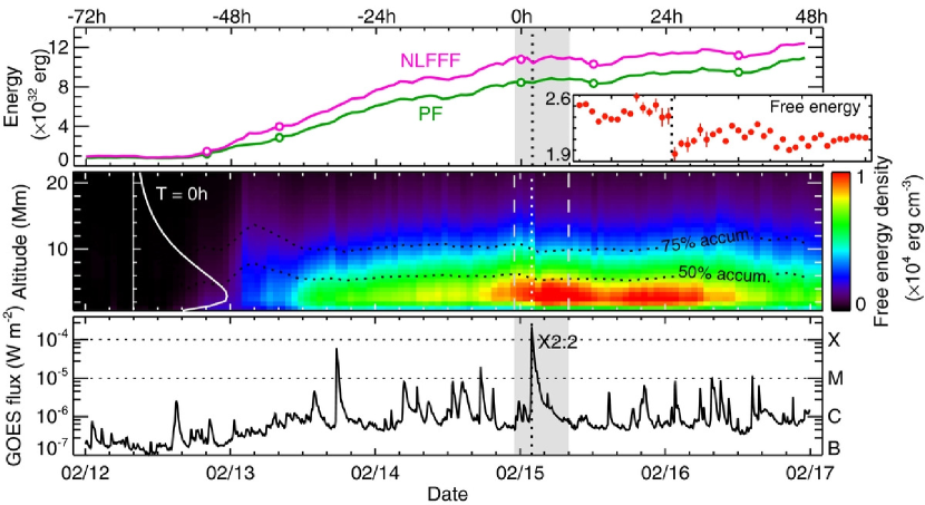
Figure 15: (a) Temporal evolution of the total (pink solid line; estimated from a NLFF model) and potential (green solid line) magnetic energy stored in the coronal volume above AR 11158 during five days. The inset shows the evolution of the free magnetic energy (that is the excess energy over a current-free field) around the time of an X-class flare (indicated by the vertical dotted line). One can clearly see the more or less continuous increase in magnetic energy, predominately caused by an emerging flux rope ($\approx 10^{26}$ J during $\approx$ 48 hours). (b) Height profile of the associated average free magnetic energy. The white curve shows a sample altitude profile of the average free energy on February 15 at 00:00 UT. The course of each profile over time and over height is visualized by the color code shown. Black, more or less horizontally running, dotted lines indicate the iso-contours of 50% and 75% of the total free energy. (c) Measured full-Sun GOES 5-min SXR flux in the 1 Å to 8 Å channel for the same time range. The vertical, white-dashed lines in (b) as well as the gray-shaded area in (a) and (c) mark the duration of an X2.2 flare. The peak time of the flare, on February 15 at 01:56 UT, is indicated by a vertical dotted lines. (Adapted from Figures 4 of Sun et al. 2012b. © AAS. Reproduced with permission.)

4.5.2 Relation to flare productivity

Depending on the magnetic field topology and its temporal evolution, very different amounts of magnetic energy are stored in time intervals of various lengths. Force-free modelling suggests energy storage rates of a few $10^{23}$ J h^-1 to a few $10^{25}$ J h^-1 (Thalmann and Wiegelmann, 2008; Sun et al., 2012b; Malanushenko et al., 2014; He et al., 2014, and see also Figure 15a). Besides, such modelling suggests that magnetic energy is stored mainly in the low solar atmosphere, possibly only a few Mm above photospheric levels (Thalmann and Wiegelmann, 2008; Sun et al., 2012b, also cf. Figure 15b).

The size and frequency of eruptive events appears to be related to the portion of the previously stored magnetic energy that is actually available for release at a given time (Choe and Cheng, 2000; Jing et al., 2010; Tziotziou et al., 2012). This so-called “free magnetic energy” is the energy difference between a NLFF and a current-free field. One generally finds a higher free energy content prior to larger eruptive events and a small amount of free energy ($\lesssim 10^{23}$ J) prior to the weakest flaring activity (Gilchrist et al., 2012), where “weakest” activity refers to smaller than C-class events. A free energy of $\approx$ $10^{24}$ J to $\approx$ $10^{25}$ J has been reported prior to weak flaring activity (Bleybel et al., 2002; Régnier and Priest, 2007; Thalmann et al., 2008; Sun et al., 2012a), where “weak” means C-class flares. Moderate to strong (M- to X-class) events tend to occur only when free energies of some $10^{25}$ J to some $10^{26}$ J are present (Régnier et al., 2005; Metcalf et al., 2005; Thalmann and Wiegelmann, 2008; Jing et al., 2009; Sun et al., 2012a; Feng et al., 2013). Note, however, that the build-up of a sufficient amount of energy on its own does not guarantee the occurrence of a subsequent eruption and the release of part of this energy (Gilchrist et al., 2012).

4.5.3 Energy release

The release of magnetic energy is believed to take place in current sheets, very limited regions where magnetic field and plasma are locally decoupled. This allows the magnetic field to diffuse and change its topology by means of magnetic reconnection (see section 4.2.2). It has been contended by Moore et al. (1995) and Lin et al. (2009) that the width of these regions is $\approx$ 0.1 Mm to 1 Mm. Narrower current sheets, as proposed by Wood and Neukirch (2005), would result in even smaller diffusion time scales. Clearly, unlike the global magnetic diffusion time-scale of several months, the diffusion time scale in currents sheets is very small ($\tau_{d}\approx$ 1 s to 10 min). In other words, the presence of current sheets in the corona, permits the efficient release of magnetic energy on active-region scales, in contrast to the non-efficient magnetic diffusion on global scales. Due to the rarity of vector magnetic field measurements in the corona, direct observational detections of current sheets are restricted basically to the upper chromosphere. From observations, only an upper limit of roughly 1 Mm can be given on the width of current sheets (Solanki et al., 2003).

Force-free models of ARs indicate that the height where the gross part of the magnetic energy is released is located $\lesssim 20$ Mm above the photospheric level (Thalmann and Wiegelmann, 2008; Sun et al., 2012b). Only a fraction of the released free energy goes into the acceleration of particles. Heated and/or accelerated, particles propagate from the reconnection site, near the apex of the coronal loop, downwards along the legs of the loop to the chromosphere, where they loose their energy due to collisions with the denser chromospheric material. That, in turn, is heated and convected upwards and fills the newly reconnected field lines with chromospheric and transition region plasma heated to coronal temperatures, emitting in SXRs (Neupert, 1968).

Just as the free energy content prior to observed eruption is related to the flare class, one would expect that the actually released amount of free energy relates to the flare class too. Recent studies, however, do not show a clear tendency, i. e., no clear trend of more energetic events consuming more of the previously stored energy. So far, the estimated upper limits for the decrease of free magnetic energy range from 5% to 50% (Thalmann and Wiegelmann, 2008; Thalmann et al., 2008; Jing et al., 2009; Sun et al., 2012b; Feng et al., 2013). Cases were also reported without a clear decrease (Sun et al., 2012a) or even an increasing free energy (Metcalf et al., 2005, and references therein). However, there have been doubts about the reliability of the latter owing to very uncertain estimates. Often also a decrease of the free energy occurs already before the time of the peak SXR flux of a flare, and in other cases this has been seen even before the flare onset (Jing et al., 2009; He et al., 2014).

Recently, Feng et al. (2013) investigated the partition of magnetic energy during an X-class and CME event. The radiative energy release estimated from the recorded flare emission was found to be at least one order of magnitude lower than the upper limit of available free magnetic energy; this also held for the kinetic and potential energy of the associated CME and confirmed the general consensus that by far not all of the free energy is released even during the most energetic events, but that a considerable portion remains available to power successive eruptions (see also Figure 19). As discussed for the helicity budget on a global scale (see section 3.4), a non-potential magnetic field is never found to relax to a corresponding current-free configuration, in the course of an eruption. Despite expected in terms of helicity conservation, a non-potential coronal field may never entirely relax to a corresponding constant-alpha (preserved helicity) state due to the line-tied nature of the coronal structures (Antiochos and DeVore, 1999). Besides, newly emerging flux also permanently disturbs the relaxation process.

4.5.4 Coronal implosion and photospheric response

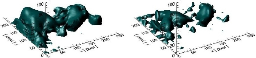
Figure 16: NLFF magnetic field model of the active-region field above NOAA AR 10540 (a) before and (b) after a large M-class flare. Iso-surfaces of a absolute magnetic field strength of 200 G are shown. The iso-surfaces give an impression of the magnetic pressure, sustaining different parts of the AR. It is evident that various areas within the AR react with different sensitivity to the flare, i. e., show differently strong signatures of implosion. (Adapted from Figure 3.7 of Thalmann (2010). Reproduced with permission.)

The release of magnetic energy naturally leads to a deviation from the previous balance of the magnetic forces in an AR. The magnetic pressure is directed towards weaker magnetic fields, i. e., generally pointing upwards towards higher altitudes and competes with the magnetic tension that tries to reduce the curvature of the magnetic field lines. The rapid release of energy during an eruption may cause a reduction of magnetic pressure, accompanied by a deflation of the magnetic field, termed “coronal implosion” (Hudson, 2000, and see Figure 16). Model calculations by Janse and Low (2007) confirmed that if the post-eruption thermal pressure cannot compensate for the eruption-related magnetic pressure reduction, a magnetic system will implode.

Frequently, observational evidence for such implosions is found in the form of the contraction of observed coronal loops (Liu et al., 2009a; Liu and Wang, 2009; Sun et al., 2012b; Gosain, 2012; Simões et al., 2013). Liu et al. (2012) claimed that the apparent loop contraction is not just a projection effect. This conclusion, they argued, was possible due to their observation of the contracted coronal loops to reside at lower heights than those of the pre-flare system (see Figure 17 and also Liu and Wang, 2010). Importantly, the magnetic field lines after an eruption never regained their pre-flare heights. Almost all of the studied eruptions showed both contracting overlying large-scale loops that are observable in cooler EUV channels, and expanding components underlying, newly-reconnected field lines, preferentially visible in warm/hot EUV channels. However, even before the conventional large-scale expanding motions could be seen for particular flares, contracting motions during the impulsive phase of flares were observed in the form of descending motions of loop-top sources (Krucker et al., 2003; Joshi et al., 2009) and EUV flaring loops (Li and Gan, 2006; Liu et al., 2009a), along with converging H$\alpha$ ribbons or HXR footpoints. Ji et al. (2007) explained the observational aspects related to the initial contraction in terms of the relaxation of a modelled highly-sheared core field. They formed new field lines, still highly sheared and containing much of the non-potential energy. The dissipation of free energy causes the sheared field to relax and contract; their effect is much stronger than the expansion effect by reconnecting arcade field lines during the initial phase.

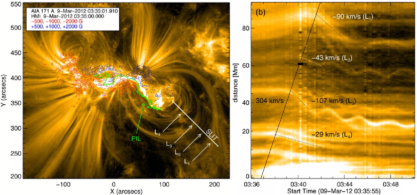
Figure 17: (a) SDO/AIA image of the 171 Å emission of NOAA AR 11429 on 2012 March 9. The blue/red contours resemble the co-temporal negative/positive LOS component of the photospheric magnetic field measured with SDO/HMI. The green line marks the PIL. The white line indicates the slit along which the motion of four well-defined bundles of coronal loops (L₁ to L₄) is investigated. (b) Time-position diagram during the impulsive phase of an M6.4 flare. Shown is the projected speed of the coronal loop bundles which contract with different apparent speeds. A delay of the implosion onset with height is clearly visible and indicated by the inclined black straight line. (Adapted from Figures 1 and 2 of Simões et al. (2013). © AAS. Reproduced with permission.)

The deflation of coronal loops, caused by the release of magnetic energy, is often also accompanied by changes of the shear of the horizontal component of the photospheric magnetic field. The sign of this change remains inconclusive, however, since both, an increase of the shear (Wang, 1992; Chen et al., 1994; Wang et al., 1994; Liu et al., 2005; Petrie, 2012; Wang et al., 2012a, b), as well as a decrease has been found during flares (Wang, 2006). To explain such contradictory results, Dun et al. (2007) proposed that the measures for the non-potentiality of a magnetic field may take on different values from one portion of an AR to another. Findings may then depend on the specific choice of the analysed photospheric area. Moreover, projection effects due to the location of the investigated area on the solar disk might also result in changes of the observed longitudinal field, similar to that expected for flare-related reconfigurations (Wilkinson et al., 1989; Venkatakrishnan et al., 1989; Spirock et al., 2002). We also point out the need to check carefully to what extent the determined magnetic field configuration is affected by the thermal and velocity structure of the atmosphere (see review by Solanki, 1993) by weak blends in the employed spectral lines, or by instrumental effects. Finally, as recently speculated, the magnetic field may behave differently at different altitudes with varying domains of increasing and decreasing shear (Jing et al., 2008; Sun et al., 2012b). No unique mechanism accounting for all of these observed aspects of magnetic shear has so far been identified.

4.6 Magnetic helicity budget

The storage of magnetic energy in the coronal volume above ARs is accompanied by an accumulation of magnetic helicity (see section 3.4 for the Sun’s global helicity budget and section 5.2.6 for a corresponding discussion on quiet-Sun fields). Often, also the current helicity is investigated, this quantifies how much the fields are locally twisted (Démoulin, 2007). In contrast to magnetic helicity, the current helicity is not a conserved quantity; the general relationship between the two is not known (van Driel-Gesztelyi et al., 2003). Within this work, we restrict ourselves to the discussion of magnetic helicity.

4.6.1 Helicity build-up and storage

Any magnetic helicity gained by a dynamo action somewhere within the convection zone during the generation of magnetic field is transported into the solar atmosphere by the emergence of helical magnetic flux tubes in the photosphere (Seehafer, 1990). The flux of magnetic helicity at photospheric levels is the result of the combined effect of the motions of magnetic structures due to convective plasma flows and the subsequent advection of these helicity-carrying structures. For a review on observations and modelling of the helicity at photospheric levels see Démoulin and Pariat (2009). The photospheric motions that twist and/or shear the magnetic flux tubes result in the coronal magnetic field to gain even more helicity.

Investigating the helicity injection rate in ARs by shearing motions only requires the knowledge of the normal component of the magnetic field and the horizontal velocity of the magnetic elements within an AR (Berger, 1984; Démoulin and Berger, 2003; Chae et al., 2004). The resulting estimate is thus a mixture of the enhancement of the helicity content by shearing motions and the portion of helicity emerging from below the photosphere. Magara and Longcope (2003) proposed that the helicity contribution from the vertical flows might only dominate early phases of flux emergence, followed by a dominant contribution from the shearing flows in the later stages of an evolving AR. This is in the opposite of what has been presented recently by Liu et al. (2014) who analysed the ARs during their emergence phases and found that shearing motions contribute the most to the ARs’ helicity content.

And also other contributions to the helicity budget within an AR were detected, including the rotational motion of sunspots around their own axis, which results in enhanced magnetic twist. The rotation of the center of one polarity around the center of the reversed polarity center also adds to the writhe of a magnetic flux tube’s axis (Tian and Alexander, 2006; Tian et al., 2008; Kumar et al., 2013). Liu and Zhang (2006) estimated the accumulation of helicity associated to the rotation of a pair of bipolar sunspots (during about 31 hours) to be $\approx 2\times 10^{42}$ Mx². They noted another increase of $\approx 3\times 10^{43}$ Mx² during a following period of $\approx 96$ hours, while strong shearing motions were observed. Zhang et al. (2008) estimated the helicity injected by the rotational motion of sunspots around their centers within an AR to be $\approx$ $10^{43}$ Mx², which was on the same order as the combined contribution by shearing motions and flux emergence.

The above discussion underlines that further detailed research on evolving ARs is needed in order to disentangle the contribution of emerging, shearing and rotational motions and to assess their importance for the total helicity content of ARs. Importantly, Vemareddy et al. (2012b) showed that such estimates depend on the time interval between successive magnetic vector maps and the window size within which the horizontal footpoint velocities are tracked. Correspondingly, they guessed the general uncertainty of calculated helicity injection rates and total helicity accumulations to be $\approx$ 10%. Vemareddy et al. (2012a) found evidence that individual portions of an AR contributed differently to the total helicity content. While in one part an accumulation of negative helicity was recorded, an injection of positive helicity was found in another part. Vemareddy et al. (2012b) recognized that major flaring activity only occurred at times when helicity was injected in the AR with a sign opposite to the dominant sign of the AR (see also Kusano et al., 2002). Similar findings have been presented for CME- (Wang et al., 2004b) and MC-productive (Chandra et al., 2010) ARs. For these too, the sign of the helicity inherent to the newly emerging magnetic flux systems may well be opposite to that of the dominant helicity in the preexisting active-region magnetic field.

4.6.2 Relation to flare productivity

The rates of injected magnetic flux and helicity are necessarily related to each other (LaBonte et al., 2007; Tian and Alexander, 2008; Park et al., 2008; Chandra et al., 2009; Tziotziou et al., 2012). The flare productivity, however, may be more closely related to magnetic helicity injection than to the amount of injected magnetic flux (or stored magnetic energy). More precisely, if positive and negative helicity is injected at the same time at approximately the same rate in flare-productive ARs, the absolute helicity flux (transported into the atmosphere by emerging motions) correlates well with the SXR flux (Maeshiro et al., 2005, and see Figure 18). Park et al. (2010) based a similar conclusion on the observation that for flaring ARs with a large unsigned magnetic flux, the average helicity injection rate was twice that of non-flaring regions. In fact, a systematic study by LaBonte et al. (2007) on the helicity injection in ARs showed that all X-class flares were associated to peak helicity fluxes greater than $6\times 10^{36}$ Mx² s^-1 and consequently proposed a causal link of the peak helicity flux to the ability of an AR to produce an X-class flare.

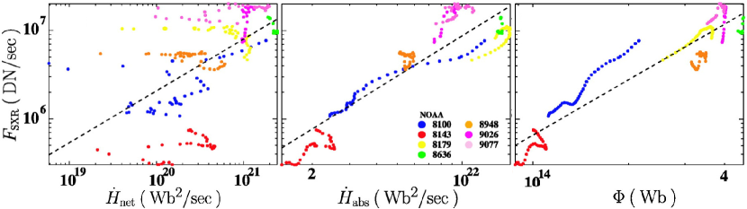
Figure 18: Time-averaged (a) net helicity flux, $\dot{H}_{\rm net}$, (b) absolute magnetic helicity flux, $\dot{H}_{\rm abs}$, and (c) unsigned magnetic flux, ${\rm\Phi}$, as a function of the SXR flux, $F_{\rm SXR}$, of seven ARs. The SXR flux is estimated from the measured intensity Yohkoh/SFD images by integration over the area used for helicity calculations and corresponds to the Yohkoh data number (DN) per second, where 1 DN corresponds to 100 electrons in the CCD detector. Time averages are taken over 24 h. Values corresponding to NOAA ARs 8100, 8143, 8179, 8636, 8948, 9026, and 9077 are represented by blue, red, yellow, green, orange, magenta, and pink dots, respectively. The dashed line represents a regression line, obtained from a least-squares method. One can see that the absolute helicity flux correlates better with the SXR flux than does the net helicity flux for the individual ARs. Note that for all ARs except 8143 and 8636 repeated flaring activity (C-, M- or X-class) has been reported. (Adapted from Figures 3 and 8 of Maeshiro et al. (2005). © AAS. Reproduced with permission.)

This proposal raises the question whether or not there is a “critical” amount of helicity which, once reached, favours the onset of an eruptive process. Park et al. (2008) found a nearly constantly increasing coronal helicity, preceding all of the considered 11 X-class flares. Importantly, they suspected an individual critical limit of accumulated helicity for each of the eruptive ARs, since they could not identify a common threshold for all events. Park et al. (2010) compared the magnetic properties and flaring activity for a sample of 378 ARs. They note that prior to all flares with a peak SXR flux of more than $5\times 10^{-5}$ W m^-2 a significant amount of helicity ($10^{42}$ Mx² to $10^{43}$ Mx²) was monotonically accumulated during 12 h to 48 h. Analysing more than 150 ARs, Tziotziou et al. (2013) found that a relative helicity of $\approx 10^{42}$ Mx² and $\approx 10^{43}$ Mx² is accumulated prior to M- and X-class flaring, respectively. Note that whenever we speak of “relative” helicity, the helicity of a non-potential field with respect to that of the corresponding potential field is meant. Earlier already Tziotziou et al. (2012) had estimated the instantaneous magnetic energy and helicity budgets of ARs and found that those with a free energy of $\lesssim 4\times 10^{24}$ J and a relative helicity of $\lesssim 2\times 10^{42}$ Mx² were not flare-productive. Also, the flare class of the observed events was successively smaller (X- to C-class) for ARs with successively less free energy and relative helicity budgets. Early estimates of the helicity budget of flare and CME-productive ARs, based on force-free field models, range from $\approx 10^{34}$ Mx² to $\approx 10^{43}$ Mx², with the general tendency that ARs with a higher helicity content are more flare productive (Régnier et al., 2002; Régnier and Canfield, 2006; Régnier and Priest, 2007).

In recent years, considerable effort has been invested into developing methods that infer the coronal helicity budget based on the reconstructed NLFF coronal magnetic field. This is far from trivial, since it often involves the computation of the magnetic vector potential that has to satisfy specific gauge properties (Rudenko and Myshyakov, 2011; Thalmann et al., 2011; Valori et al., 2012a; Yang et al., 2013). So far, these models have not been applied to real solar cases, but have been tested by use of semi-analytic force-free magnetic field solutions. Only Valori et al. (2012b) investigated the helicity content of an AR during flux emergence and found a relative helicity of $\approx 10^{42}$ Mx² prior to background, i. e., B-level flaring activity. The hesitation to apply the developed methods certainly arises from the strong influence the choice of a particular gauge as well as its numerical implementation may have on the model outcome, especially when applied to real data. Only when the reliability of such methods has been assessed, will it become clear, whether summing over the helicity injected at a photospheric level, i. e., estimated from routine direct photospheric magnetic field measurements, represents the safest estimate of the coronal helicity content (Démoulin and Pariat, 2009).

4.6.3 Helicity dissipation and transport

In contrast to dissipating magnetic energy, magnetic reconnection is a very inefficient process for removing magnetic helicity. This was shown by Berger (1984), who had tested the magnetic helicity decay in a coronal loop, by assuming classical anomalous conductivity in a circular loop with a length of 100 Mm, a radius of 10 Mm, and an uniform temperature of 1 MK. He found a diffusion time scale of $\approx 10^{9}$ s to $10^{13}$ s, which is far too long to be relevant for time scales of impulsive (eruptive) processes such as flares, where typical time scales are $\approx 10^{3}$ s. Instead, during magnetic reconnection, and on time scales relevant for it, the magnetic helicity is approximately conserved. Only its source, the mutual linking of different flux systems or the internal twist of a magnetic structure, is transformed (Hornig and Rastätter, 1997). This provides a constraint on the relaxation of a current-carrying magnetic-field configuration by energy dissipation: it can only relax to another lower-energy, still current-carrying state but not to a current-free one (Woltjer, 1958; Taylor, 1974; Bellan, 1999, 2006). Importantly, the decrease of both magnetic helicity and of magnetic energy due to an eruption is often temporary and sets in before the onset of the eruptive event, as defined by the impulsive rise of SXR emission (Jing et al., 2009; Tziotziou et al., 2013). Both are often found to return to, or even exceed the pre-eruptive level within hours, thus allowing for subsequent flaring activity (see Figure 19).

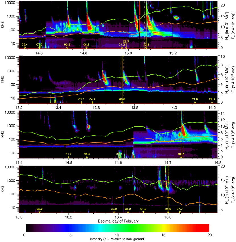
Figure 19: Relative helicity (green curves) and free magnetic energy (orange curves) of AR 11158 in February 2011, around the times of four large eruptive events (with values are averaged over 72 minutes): (a) an X2.2 flare of February 15, (b) an M6.6 flare on February 13, (c) an M2.2 flare on February 14, and (d) an M1.6 flare of February 16. The flare onset, peak and end times (defined by the GOES SXR flux) are indicated by dotted, solid and dashed vertical lines, respectively. The color-coded background resembles the co-temporal WIND/WAVES frequency-time radio spectra. It can well be seen that a decrease of the magnetic energy and relative helicity magnitude starts before the onset of the flares and displays a gradual, rather than instantaneous character. (Figure 11 of Tziotziou et al. (2013). © AAS. Reproduced with permission.)

As a consequence of the conservation properties of magnetic helicity, a change of the coronal magnetic helicity content can only be caused by an expulsion of a magnetic structure and its inherent helicity, such as a CME to interplanetary space. A typical CME contains a magnetic helicity on the order of $10^{42}$ Mx², as this is also a the typical magnetic helicity content of a MC (DeVore, 2000; Georgoulis et al., 2009, and see also section 3.4). These estimates agree very well with the helicity budget of ARs prior to major eruptions ($\gtrsim 2\times 10^{42}$ Mx²; see Tziotziou et al., 2012, and see section 4.6.1). MCs often show the same chirality as their source region, as inferred from the twist of the flux tubes they originate from (Rust, 1994; Mandrini et al., 2004). But events have also been reported where this has not been the case. For instance, Chandra et al. (2010) investigated a case in which observed features (sunspot whorls and flare ribbons) as well as a corresponding LFF magnetic field suggested a predominantly negative helicity within an AR. In contrast, the associated MC was attested a positive helicity, which contradicted helicity conservation. Only a very accurate analysis of the helicity injection revealed that a strong, local injection of positive helicity served as the source for the observed positive helicity of the MC.

Note that already Kusano et al. (2004) outlined the importance of neighbouring flux systems of helicity with opposite signs within a single AR for its flare productivity. And Leamon et al. (2004) attested only models invoking magnetic reconnection between the small-scale active-region magnetic fields and their overlying large-scale envelope field, where the latter ejected an MC, the ability to relate their helicity aspects correctly.

5 Quiet-Sun magnetic fields

Traditionally the “quiet Sun” regions got their name because they were assumed to lack activity. However, while large-scale eruptions are mainly associated with ARs (see section 4), the QS is not quiet either. Dynamic processes that occur on smaller scales had simply not been resolved by early missions and instruments. Already Labonte (1979) pointed out that the total magnetic flux of the QS exceeds the flux contained in ARs by far and that it drives activity, such as spicules. These were first observed in H$\alpha$ and described as “small spices of chromospheric material” (Roberts, 1945). Ephemeral ARs (see section 1.1.1) were also found to be centers of activity Harvey and Martin (1973). As in their active-region counterparts, the photospheric magnetic field in the ephemeral regions drives activity, such as X-ray bright points, (Golub et al., 1974, 1977; Priest, 1994) in the upper solar atmosphere.

5.1 3D magnetic field structure in the quiet Sun

Because of the often mixed magnetic polarities on smaller scales in the QS, we mainly find magnetic loops which are very short and hardly reach into higher layers of the solar atmosphere. With modern high-resolution measurements, however, we can use magnetic field modelling techniques to model the 3D structure in the QS, similar to those described in section 2.2 and which are routinely applied to the active Sun (see section 4). Nevertheless, some care has to be taken, as is discussed in section 5.2.5.

Because of their easier computational load and because only photospheric LOS measurement are required as boundary condition, the topology of the quiet Sun’s outer atmosphere and its temporal evolution is usually investigated by use of potential field models. However, one has to keep in mind that any static-model approach provides only a snapshot of the, in reality dynamic, magnetic carpet. Schrijver and Title (2003) modelled the fraction of magnetic flux that connects from network elements into the upper solar atmosphere and found it to scale with the flux density of the underlying internetwork field. For relatively strong internetwork flux densities, on the order of $5\times 10^{-3}$ Wb m^-2, only about 30% to 40% of the flux connects to the corona while the greater part connects back down in the form of closed loops.

5.1.1 Photospheric quiet-Sun loops

The structure and dynamics of the quiet-Sun magnetic field can be investigated with spectro-polarimetric measurements. Martínez González et al. (2007), using data from VTT, found low-lying photospheric magnetic loops connecting about 10% to 20% of the visible magnetic flux of opposite polarity. Note that emerging small-scale loops are observed in the form of newly detected horizontal fields well before vertical flux is detected (see Centeno et al., 2007, for a corresponding study based on Hinode/SOT-SP data). In subsequent studies, Martínez González and Bellot Rubio (2009) and Martínez González et al. (2010) presented observations of emerging ${\rm\Omega}$-loops by combining magnetic and imaging data from Hinode/SOT and DOT. With an even higher resolution, based on the balloon-borne Sunrise/IMaX instrument, Danilovic et al. (2010a) investigated a large number of transverse photospheric features. The high-resolution IMaX data revealed that 97% of these features are smaller than the mean size of such structures ($\approx$ 1$.\!\!^{\prime\prime}$0 squared) found in earlier studies.

Already Isobe et al. (2008) had detected emerging $\rm\Omega$-shaped loops. They showed that such structures, after emergence, reach the chromosphere and reconnect with the mainly vertical fields there. Thus they contribute to the heating of the chromospheric plasma there and to generating coronal MHD waves. These high-frequency waves may then contribute to coronal heating and the acceleration of the solar wind particles. For a description of the kinetic processes involved in coronal heating, we refer to specialized reviews such as that by Marsch (2006).

5.2 Associated photospheric fields and the response on the upper atmosphere

QS structures are quite dynamic, as new magnetic flux permanently emerges, usually in bipolar form. The corresponding loops connecting the two polarities emerge into the solar atmosphere, while the loop footpoints move apart due to the shape of the rising loop. The footpoints also undergo displacement due to horizontal photospheric motions. The opposite polarity footpoints keep separating until eventually one or both cancel with older photospheric magnetic flux (Martin et al., 1985). As a consequence, the magnetic flux in the quiet-Sun photosphere is replaced every $\approx$ 14 hours (Hagenaar, 2001). An important question is, how the corona responds to these changes in the photospheric field and how we can get insight into the quiet-Sun field in the upper solar atmosphere. This was addressed by Close et al. (2004, 2005) using potential field modelling based on photospheric SOHO/MDI LOS magnetograms. They found that the coronal magnetic field becomes redistributed even faster, with a typical time of 1.4 hours.

5.2.1 Doubts about the concept of a magnetic canopy

The concept of a magnetic canopy (Gabriel, 1976, and see section 1.3.1), in the sense of a horizontal magnetic field that fills the upper chromosphere and overlies a most field-free atmosphere, is still a subject of debate. One problem is that there are multiple definitions of a canopy. One is that it is nearly horizontal field overlying largely field-free regions. Another is that it is a horizontal boundary between the $\beta>1$ and $\beta<1$ field. Instead of vertically more or less well divided domains of high or low $\beta$, such domains may well be mixed up, even “islands” may exist (Rosenthal et al., 2002).

A number of comparative studies of magnetic field structures and/or bright emission from photospheric levels, and corresponding signatures from higher atmospheric layers, revealed no obvious expansion of the magnetic network with height (see section 1.3). Zhang and Zhang (2000a, 2000b), for instance, compared quiet-Sun magnetic signatures inferred from Fe i 5324 Å (photosphere) and H$\beta$ 4861 Å (chromosphere) observations and found no significant change of the magnetic configuration over a height of $\approx$ 1.5 Mm. They emphasized, however, that the H$\beta$ line exhibits high noise levels so that the expansion of the magnetic features might simply be hidden by the noise. Peter (2002), among others, presented SOHO/SUMER C i continuum (chromosphere) and O vi 1037 Å (transition region) brightness observations which revealed network elements of nearly the same size. This observation can be construed to contradict the concept of a nearly horizontal canopy at a height of $\approx$ 1 Mm above the photosphere, or alternatively, it implies that the brightness structures may expand less rapidly with height than the magnetic field. Using TRACE 171 Å observations, already Zhang et al. (1999) had found that the width of the emission associated to fibrils was nearly the same at different heights: at their photospheric root as well as $\approx$ 30 Mm higher up in the atmosphere. It was speculated as a possible explanation that, either the observed emission might not be sensitive to the detection of the desired canopy structure – as recently supported by Peter and Bingert (2012), see section 1.4.2 for details – or that network-fields in the QS could, by some mechanism, be prevented from fanning out (Zhang, 2005). These claims would imply that the need for an extra force, at least as strong as the horizontal pressure gradients, that prevents the magnetic field from expanding with height. At least in photospheric layers, magnetic structures and the bright points associated with them are seen to expand with height (Briand and Solanki (1995) and Bühler et al., 2014, Astron. Astrophys., submitted).

Schrijver and van Ballegooijen (2005) modelled the quiet-Sun network magnetic field at heights of $\lesssim$ 20 Mm above chromospheric levels. They found an average plasma-$\beta$ close to unity in the entire simulation domain, indicating that the quiet-Sun corona is not be force-free, i. e., that the magnetic field there is not unaffected by the plasma. A magnetic canopy also suffers at the hands of atmospheric flows. Thus, Pietarila et al. (2011) demonstrated on the basis of 3D radiation MHD models that in particular downflows pull U-loops out of a magnetic canopy into the lower lying atmosphere, giving rise to some of the horizontal fields seen in the quiet photosphere. With time the canopy loses its clear identity due to this process.

The canopy separates the fields originating from the network and supposedly opening into the atmosphere from closed fields, originating and closing in the weak internetwork. In a numerical experiment, Schrijver and Title (2003) showed that strong internetwork fields allow flux densities capable of considerably modifying the dynamic geometry of the magnetic coupling between the photosphere and outer layers. They argue that bunches of field lines likely connect from strong internetwork regions well up to the corona while field lines from the network close back onto internetwork fields. They estimated that the magnetic flux which originates from internetwork fields and connect to the corona to be $\approx 50$% of the total flux of the quiet-Sun coronal magnetic fields. It may well be that in the mixed-polarity QS, canopies play a less important role than in the more unipolar environment of CHs (see Figure 27 in section 6.2.2), which is where they are generally placed in theoretical studies.

5.2.2 Network and internetwork magnetic loops

Wiegelmann et al. (2010a) used a potential and LFF magnetic field model and found that the majority of the model field lines connect strong internetwork features below equipartition field strength with network elements. They were also able to show that for most of the field lines reaching chromospheric and coronal heights, one of the footpoints is located in the strong internetwork fields. In other words, while the idea of a canopy, formed by horizontal fields above activity centers, seems well established it is more controversial for the atmosphere above quiet-Sun regions. More recently, however, observational evidence was again found by Pietarila et al. (2009) that chromospheric fibrils formed a canopy over parts of a plage region and the quiet-Sun network (see Figure 20). They point out that this might not even contradict the finding of Schrijver and Title (2003) – namely, that internetwork fields disable the formation of a large-scale canopy – but instead, that the apex of small-scale loops of the internetwork may not always reach a height in the atmosphere where a canopy might exist. And indeed, potential and force-free magnetic field extrapolations carried out by Wiegelmann et al. (2010a) showed that the number of short field lines (with apex heights of $\lesssim$ 500 km) outnumber the field lines reaching the corona (with apex heights $\gtrsim$ 2.5 Mm). It has to be noted, however, that a rather small portion of the solar atmosphere was investigated in this study (based on the limited Sunrise/IMaX FOV), so that a possible bias cannot be ruled out.

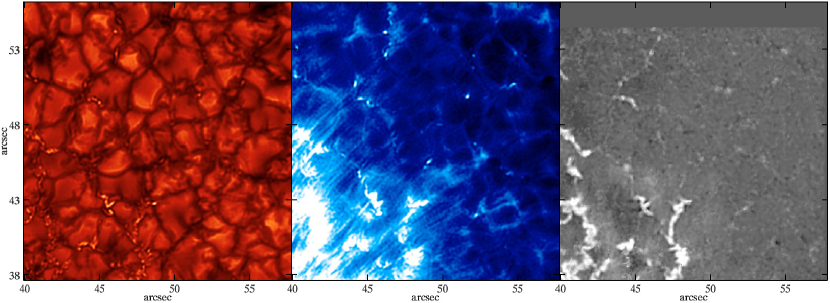
Figure 20: (a) Continuum image, (b) Ca ii K intensity and (c) longitudinal magnetic flux (ranging from -800 G to 1 kG) on August 9, 2007, covering a plage region and the QS seen as bright and dark areas in (b), respectively. The continuum image displays a clear pattern of dark intergranular lanes, often exhibiting emission from more or less tightly packed bright photospheric filigree. Comparison with the Ca ii K image shows that many of the observed thin chromospheric fibrils originate from the locations populated with filigree. Longer fibrils, originating near the boundary between the bright plage and surrounding (darker) QS areas indicate a canopy-like magnetic connection between areas of stronger, i. e., plage, and weak, i. e., QS, magnetic fluxes. (Figure 8 from Pietarila et al. 2009. Reproduced with permission, © ESO.)

5.2.3 Magnetic carpet

The dynamics of the QS is quite complex since the atmosphere above the magnetic network is permanently and everywhere filled with small-scale magnetic flux in the form of magnetic loops emerging from below. This small-scale magnetic mesh is usually referred to as “magnetic carpet” (Title and Schrijver, 1998, and see Figure 21). The structure of this mixed-polarity network is driven by processes such as magnetic flux emergence, flux cancellation as well the coalescence and fragmentation of magnetic elements (Parnell, 2001). Widely used for the statistical analysis of the properties of magnetic features associated with the magnetic carpet are potential and LFF field models (see section 2.2.1). Both methods are based on the observed LOS photospheric magnetic field and deliver similar results concerning the length of field lines, the height of their apex in the atmosphere and the approximate field strength (Wiegelmann et al., 2010a).

Therefore, although the evidence for a common canopy-like field (nearly horizontal field overlying a nearly field-free region) is relatively strong, the criticisms of the canopy as a boundary between open and closed field lines as well as between high and low-beta plasma are better founded. Therefore, such views of the canopy do need revising.

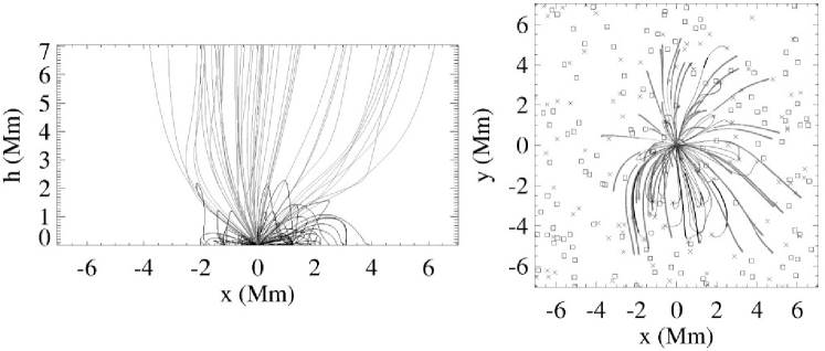
Figure 21: Illustration of the magnetic carpet, computed from a potential field model, when viewed (a) from the side and (b) from top. The plot depicts a photospheric magnetic flux concentration with a flux of $3\times 10^{8}$ Wb, surrounded by a small-scale mixed-polarity field (marked by squares and crosses for opposite polarities). The FOV reaches halfway to the neighbouring network sources. Field lines with one footpoint in the central flux concentration (closed field lines shown as black and open field lines shown as gray curves) suggest that a collar of field lines that emanates from the network and closes back onto the internetwork field within several Mm, implying that most of the coronal field is likely anchored in the internetwork field, rather than in the network. (Adapted from Figure 1 of Schrijver and Title (2003). © AAS. Reproduced with permission.)

5.2.4 Role of magnetic fields in coronal and chromospheric heating

The fact that the plasma temperature in the solar corona is a factor of $\approx 10^{3}$ higher than in the photosphere motivates the search for plausible mechanisms yielding the needed amount of energy involved. Throughout the last decade, a number of authors, including Walsh and Ireland (2003); Aschwanden (2005); McIntosh et al. (2011); Wedemeyer-Böhm et al. (2012); Winebarger et al. (2013), demonstrated that one of several mechanisms, involving small-scale X-ray jets, bright points, micro- and nanoflares as well as Alfvén and MHD turbulence and waves, are able to provide partial explanations for the extreme heating of coronal plasma. Mass and energy-transport between the lower atmosphere (photosphere and chromosphere) and the outer atmosphere (corona) is, in general, a challenging concern. Not only because of the complicated and highly dynamic structure of these layers, but also because of the highly non-linear physical processes involved. Nevertheless, some progress was made already during the Skylab-era (see Withbroe and Noyes, 1977, for a review). The discussion of coronal and chromospheric heating is well outside the scope of the present paper, however and we therefore refer the interested reader to the specialized review by Klimchuk (2006).

Numerical experiments, carried out by Schrijver and Title (2002) showed that low-lying chromospheric fields are well outlined by the magnetic connection between magnetic elements observable, e. g., in the form of H$\alpha$ fibrils. Although a complex magnetic field structure was found, which contained multiple null points representing a potential source for reconnection, they were found to reside in the low atmosphere only and thus were not likely to significantly contribute to coronal heating. Régnier et al. (2008) used a potential magnetic field model based on Hinode/SOT-SP magnetograms to investigate the relation of coronal and photospheric null points and confirmed a shortage at coronal heights. In particular, they found that 98% of the null points present in the model where located at photospheric or chromospheric heights, and only 2% were found to be situated at coronal heights (see Figure 22). Thus, they confirmed earlier findings based on numerical experiments which stated that magnetic reconnection at coronal null points is unlikely to be the source for coronal heating.

Wiegelmann et al. (2013) investigated a 22-minute time series of potential field equilibria extrapolated from Sunrise/IMaX data and found that the magnetic connectivity in the upper solar atmosphere changes rapidly, with a recycling time of $\approx$ 3 min – a short time compared to $\approx$ 14 min in the photosphere. An estimation of the upper limit for the free magnetic energy, which might be converted to heat by magnetic reconnection was still somewhat too small to be the dominant source for chromospheric and coronal heating in the QS. The same conclusion was reached by Chitta et al. (2014), based on a magneto-resistive computation starting from series of SDO/HMI and from Sunrise/IMAX magnetograms.

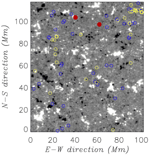
Figure 22: Spacial distribution of the projected location of magnetic null points, computed from a potential field model. Blue, yellow and red circles mark the locations of photospheric, chromospheric, and coronal nulls, respectively. The quantity of coronal nulls is outnumbered by that of the photospheric and chromospheric nulls. Photospheric magnetic field in a quiet-Sun area observed with Hinode/SOT on 24 June 2007 at 22:09 UT. The gray-scale background depicts the LOS magnetic field component, in the range $\pm$ 50 G. Black/white represents negative/positive polarity. (Figure 1 of Régnier et al. (2008). Reproduced with permission, © ESO.)

5.2.5 Force-freeness of quiet-Sun magnetic fields

Going beyond the potential field approach and applying force-free extrapolation methods (see section 2.2), to picture the magnetic field in the outer solar atmosphere above quiet-Sun regions, is tempting. This is, however, challenging, since force-free models are based on the magnetic field measurements at low atmospheric heights, i. e., routinely at photospheric, or occasionally at low chromospheric heights. Additionally, in the QS one has to deal with a poor signal-to-noise ratio of the transverse magnetic field measurements. Nevertheless, Zhao et al. (2009) aimed to compare the measured horizontal field of Hinode/SOT-SP vector magnetograms with the horizontal field component of an associated potential field model. They confirmed that the quiet Sun’s magnetic field is non-potential, that it carries significant electric currents, and that it is sheared, on average by about $40^{\circ}$ with respect to a potential field. A different approach is to employ the magneto-resistive method of van Ballegooijen, which returns force-free fields without the need of making use of the measurements of horizontal photospheric magnetic field components. This approach has been taken by Chitta et al. (2014).

The difficulty in modelling QS-related coronal magnetic fields using different NLFF methods has recently been demonstrated by Liu et al. (2011b): the results gained from the different modelling techniques deviated considerably. The problems may run deeper, since even the assumption that the magnetic field in the QS is force-free is questionable. Following, Schrijver and van Ballegooijen (2005) it is unlikely that the quiet Sun’s coronal magnetic field is force-free or even quasi-steady. One of the necessary conditions a force-free environment has to meet is that, at a given height, the surface integral $\int_{S}B_{{\rm vertical}}^{2}-B_{{\rm horizontal}}^{2}dS$ vanishes (see Aly, 1989, for details). This condition cannot be fulfilled if, on average, the (unsigned) horizontal field is much larger than the vertical one.

This means that a predominantly horizontal field cannot exist at the base of a force-free environment, and if the horizontal flux is on average about a factor of five higher (as claimed by Lites et al., 2008) the quiet-Sun photosphere is even farther away from a force-free state than photospheric active-region fields are. It should be mentioned though, that Danilovic et al. (2010b) found that a ratio closer to 1 is also compatible with observations. Obviously, Aly’s condition is not fulfilled in the internetwork photosphere where the horizontal field is on average much stronger than the vertical field, which has important implications for the reliability of force-free magnetic field reconstructions in the QS. The fact that these fields are definitely far from being force-free in the photosphere and that most of the weak (nearly) horizontal fields are the tops of very short and low-lying loops (Martínez González et al., 2007; Centeno et al., 2007; Martínez González and Bellot Rubio, 2009; Danilovic et al., 2010a) which don’t reach up to layers where the field is closer to being force-free, the impact of the plasma on the field cannot be neglected.

5.2.6 Magnetic energy and helicity budget

Despite the difficulties and limitations of applying force-free models to quiet-Sun areas (see section 5.2.5), NLFF models have recently been applied to investigate the magnetic energy and helicity budget in the QS. Tziotziou et al. (2014) performed a statistical study with a large number of quiet-Sun vector magnetograms from Hinode/SOT-SP. They found that the QS has no dominant sense of helicity (in contrast to ARs) and that both the free magnetic energy and the relative magnetic helicity are correlated with the area occupied with network elements. Consequently, the free magnetic energy and the relative helicity are correlated as well (see blue/red stars and diamonds in Figure 23, respectively). In an earlier work, Tziotziou et al. (2012) investigated these quantities for ARs (shown as yellow stars in Figure 23, for comparison). Both energy and helicity are much lower in the QS, compared to ARs, which is naturally caused by the lower magnetic flux they contain. The authors also noted that the investigated quiet-Sun areas are closer to a potential field than the ARs, which is another reason for a lower free energy in the QS. See also sections 3.4 and 4.6 for magnetic helicity investigations on global scales and in ARs, respectively.

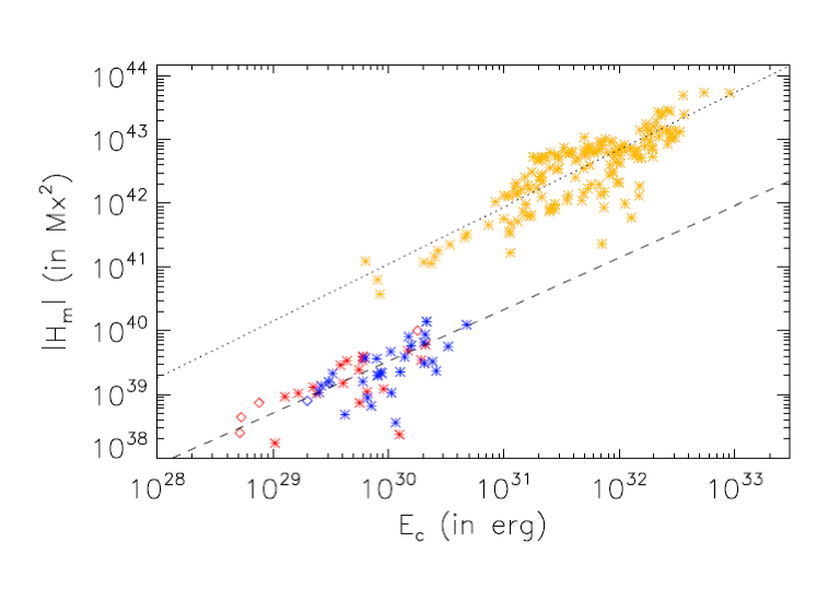
Figure 23: Free magnetic energy ($E_{c}$; horizontal axis) in relation to the magnitude of the relative magnetic helicity ($H_{m}$; y-axis). The yellow stars in the upper right part of the graph correspond to the values calculated for a number of ARs by (Tziotziou et al., 2012). Blue/red plot symbols correspond to a positive/negative total helicity budget of solar quiet regions, respectively. Asterisks and diamonds mark regions centered within $\pm$ 30^∘ heliographic latitude and higher latitudes than that, respectively. The dashed and dotted lines represent least-squares fits to the values calculated for the quiet-Sun and active-region areas, respectively. (Figure 6 of Tziotziou et al. (2014). Reproduced with permission © ESO.)

5.3 Small-scale dynamics

The observations of the coronal magnetic field show numerous dynamic phenomena on small as well as larger (active-region) scales. In particular, we now know that the term “quiet Sun” is not really adequate to describe the coronal field even outside of ARs, since numerous dynamic phenomena on small scales are known to occur there (Schadee et al., 1983; Parker, 1988; Shibata et al., 1992).

Chesny et al. (2013) found the first evidence for sigmoidal (i. e., S-shaped) loops in the QS using SDO/AIA data. These were interpreted as a clear indicator for non-potential magnetic fields. So far S-shaped loops had been observed to connect within ARs or to connect ARs on either side of the solar equator (i. e., in the form of TELs) only. S-shaped loops in the QS indicate that similar dynamic phenomena as in ARs might occur here, but on smaller scales. In fact, events similar to small versions of flares and CMEs are found in the QS (Innes et al., 2009, 2010), which mostly attract less attention than their impressive, and sometimes globally disturbing, active-region counterparts. In fact, outside of ARs the Sun displays a broad range of smaller-scale, transient phenomena which involve only a fraction of the energy that is involved in the dynamics associated to the predominant large-scale activity sites.

5.3.1 Jets

Already in the 80s of the last century, Brueckner and Bartoe (1983) reported observations of high-energy supersonic jets in quiet-Sun areas. They found that the associated shock waves reached to heights of about 4 Mm to 16 Mm. The authors applied a cloud model for the solar wind and assumed that the entire kinetic energy of the wind is provided at the Suns surface. This involves the presence of emerging flux and a field strength of 15 G and a flux emergence of $1.3\times 10^{15}$ Mx is required to power the corresponding high speed jets. In their opinion, magnetic forces are the most likely cause for the jets and a correlation to active areas in the QS was found. Moreover, the influence of the individual jets was discernible as fine structures in the solar wind flow at a distance of one AU. Later, X-ray jets were observed by Shibata et al. (1992, 1994), although not necessarily in quiet-Sun regions.

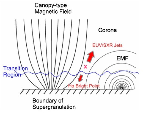
Figure 24: Schematic view on the reconnection occurring in the solar corona upon emerging magnetic flux from the center of a supergranule below with a pre-existing magnetic field. Near the reconnection X-point, the temperature is enhanced and outflows are observed presumably as EUV/X-ray jets in the corona and H$\alpha$/Ca surges in the chromosphere. (Adapted from Figure 10 of Jiang et al. (2012). © AAS. Reproduced with permission.)

Yokoyama and Shibata (1995) carried out 2D resistive MHD simulations including a simplified convection zone, photosphere, chromosphere and corona. They found that magnetic reconnection plays an important role for activity in the upper solar atmosphere and can be a common cause of both hot X-ray jets, as well as cooler loop brightening that become visible in H$\alpha$. In the former case plasma is heated up to temperatures between about 4 MK and 10 MK and is accelerated to the Alfvén speed of about 100 km s^-1. In the latter case, cool ($\approx$ $10^{4}$ K) chromospheric material is accelerated almost without plasma heating. The authors concluded that the combined energy of cool-loop brightening and hot-jet acceleration might be significantly larger than previously thought. Also the energy in loop brightenings might have been underestimated from previous observations.

The role of magnetic reconnection for heating and dynamics of the solar corona was revisited by Shibata et al. (2007), this time observationally with Ca ii H data from Hinode/SOT. So called “anemone jets” were found both in the corona and in the chromosphere. The authors interpreted the frequently observed small chromospheric anemone jets as a manifestation of ubiquitous magnetic reconnection. The coexistence of cooler chromospheric material, that becomes visible in H$\alpha$ and the hot jets expected from numerical experiments by Yokoyama and Shibata (1995) was observationally confirmed. The combined energy of these events was more than two orders of magnitude too small to explain the heating the active corona. Nonetheless, the authors pointed out that the jets observed by Hinode/SOT are only the largest events and a great number of smaller jets might have gone undetected, but may also contribute to the heating.

Recently Jiang et al. (2012) presented 2.5D MHD simulations of the processes involved in canopy-type magnetic configurations triggered by newly emerging magnetic flux into a pre-existing field configuration at the boundary of a supergranule. They found hot ($\approx$ $10^{6}$ K) and cold ($\approx$ $10^{4}$ K) jets originating from coronal microflares and associated them to what is usually observed in coronal and chromospheric images as EUV or HXR jets and H$\alpha$/Ca surges, respectively (Figure 24). That magnetic reconnection between newly emerging magnetic flux and the ambient field plays a major role for jets has been confirmed in numerical experiments recently by Moreno-Insertis and Galsgaard (2013). For a recent review on small-scale, jet-like events at chromospheric levels, we refer to Tsiropoula et al. (2012), as well as to section 6.2.4 for polar jets.

6 Coronal holes

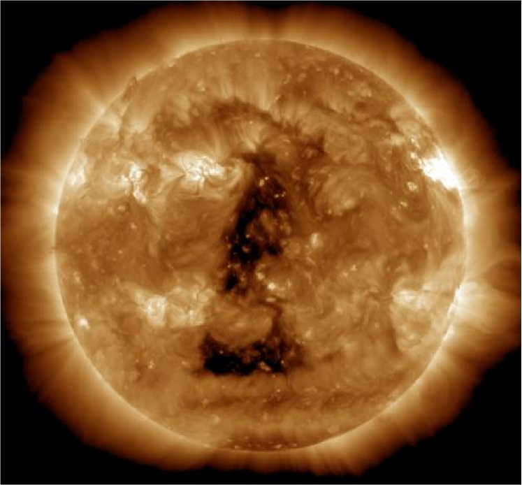
Figure 25: A large coronal hole observed with SDO/AIA at 193 Å on 13 March 2012. It can easily be distinguished from its quiet-Sun surrounding as the region of lowest EUV emission, while ARs exhibit strongest emission. Source: http://phys.org/news/2012-03-huge-coronal-hole-solar.html

CHs are regions of strongly reduced emissivity at coronal temperatures and, consequently seen as dark features in coronal images (which is why they are called “holes”; see Figure 25). The magnetic field of CHs is mainly open, i. e. organized in magnetic funnels having their footpoints in the network. Along open fields, charged particles can escape the outer solar atmosphere, leaving behind plasma of strongly reduced density and slightly reduce temperature, if compared to the quiet Sun’s corona. The main motivation for the research of CHs since the 1970s was to understand the role of CHs in terms of the mass and energy flow between the Sun’s surface and the heliosphere. For a recent overview we refer to Cranmer (2009). One distinguishes between polar CHs (PCHs) and equatorial CHs (ECHs; see Del Zanna and Bromage, 1999).

For techniques used to analyse observations of CHs, it makes a difference whether the holes are observed on the disk or above the solar limb. Discussing the corresponding challenges and issues, however, lies outside the scope of this work and we refer to the review by Cranmer (2009). Here, we focus on the magnetic field structure in CHs. As other magnetic structures on the Sun, CHs and the corresponding solar wind streams change over the solar cycle (Harvey and Sheeley, 1979). For changes of the magnetic structure of CHs in the course of the solar cycle see section 3.3.

6.1 Properties of coronal holes

6.1.1 Properties of photospheric fields associated with coronal holes

Almost continuous observations of CHs and measurements of the associated photospheric magnetic fields are available since the Skylab era in the 1970s. To our knowledge, a first review on observations of CHs and the underlying solar magnetic field was presented by Harvey and Sheeley (1979). Somewhat larger CH-averaged values, ranging from 0.8 G to 17 G, with an average value of nearly 8 G, were found by Wiegelmann and Solanki (2004). Conclusions on the magnetic structure of CHs were at that time mainly based on the photospheric LOS magnetic field observations (e. g., from KPNO). Unfortunately, at that time, the magnetic field data were subject to major uncertainties owing to systematic errors (a factor of $\gtrsim 2$). Nevertheless, it already became clear that the photospheric field in which CHs are rooted is dominated by fields of a single polarity, i. e., either positive or negative. In ECHs, for instance, the main polarity of the holes dominated in the range of 58% to 95% and, on average, 77% $\pm$ 14% (Wiegelmann and Solanki, 2004). Equatorial quiet Sun regions where approximately flux-balanced in the range of 2% to 29% and, on average, 9% $\pm$ 9%. The magnetic field strength of these photospheric fields, averaged over the whole CH, was found to lie in the range 0.5 G to 7 G (Harvey and Sheeley, 1979, and references therein). It is noteworthy that there is some scatter in the values found, depending on the observations used for analysis.

As in ARs and in the QS, reliable magnetic field measurements are mainly available at photospheric levels. Because of the poor signal-to-noise ratio in weak-field regions, it is difficult to measure the weak transverse field with high accuracy. As a consequence, observational studies and coronal magnetic field models are often based on LOS magnetic field measurements. An additional problem arises for the observation of CHs in polar regions, where foreshortening effects cannot be neglected (since the spatial resolution in the direction to the limb decreases) and where limb darkening can also become an issue.

6.1.2 Modelling of coronal-hole magnetic fields

Similar to the QS and global magnetic fields, potential field models based on photospheric field measurements are used as a first approximation of the magnetic field in CHs. Note, however, that also when applied to model the magnetic field in coronal-hole areas potential field models have their limitations (see section 5.2.5 for details). The magnetic field structure of CHs is often also studied with the help of PFSS models (see sections 2.2.1 and 3.1). In their output, coronal-hole areas are easily identified by their open magnetic fields (i. e., field lines connecting the photosphere with the source surface). A powerful tool for CH-investigations is the combination of flux-transport models in the photosphere and coronal field modelling with PFSS (see section  2.3.3 for a description of the method and section 6.3.1 for an application to ECHs).

Wang (2009) pointed out that coronal-hole areas can be reasonably well reproduced over the entire solar cycle when assuming the source surface of a PFSS model to be located at a constant height of 2.5 solar radii (i. e., $\approx$ $1.74\times 10^{9}$ m) above the photosphere. The main contribution to the open flux in PFSS models arises from the dipole and quadrupole moment of the Sun’s global magnetic field – the latter, especially around solar maximum. Higher order multipoles decrease too rapidly with height in order to contribute significantly at the source surface. Note that taking the quadrupolar field into account does not substantially change the resulting rotational properties of the coronal-hole associated magnetic field: the photospheric field (represented by the high-order multipole moments) rotates differently while the coronal field (characterized by the low-order multipoles) rotates almost rigidly.

6.2 Polar coronal holes

During solar activity minimum, large CHs occur in the polar regions as a consequence of the dominating dipolar moment of the Sun. One has to keep in mind, however, that all measurements concerning near-polar areas, are carried out from the ecliptic, i. e., from a highly inclined viewpoint with respect to the target region. With the launch of the Solar Orbiter mission, scheduled for 2017, this drawback will finally be overcome.

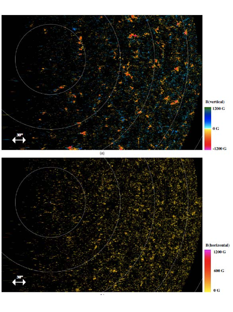
Figure 26: Maps of the signed strength of the (a) vertical and (b) horizontal components of the magnetic field vector on 25 September 2007, converted to a view from above the north pole of the Sun. East/west is to the left/right. The pixel size is $0\mbox{$.\!\!^{\prime\prime}$}16$. Black areas mark locations where the magnetic field strength has not been obtained, because the associated polarization signal did not exceed a given threshold above the noise level. The color-code in (a) represents the signed strength of the vertical magnetic field, with red/blue representing negative/positive polarity. Many of the horizontal field concentrations in (b) are co-located with the vertical field patches in (a). (Figure 4 from Ito et al. (2010). © AAS. Reproduced with permission.)

6.2.1 Magnetic flux in polar coronal holes

Hinode/SOT-SP provided the capability of studying the full photospheric magnetic-field vector around the Sun’s south polar region (Tsuneta et al., 2008a). Unipolar, vertical flux tubes with kG fields, scattered all over the PCH (ranging from 70^∘ to 90^∘ solar latitude) and ubiquitous horizontal fields were found. The strong (kG) vertical spots are unipolar, while the average field strength of the entire FOV is only about 10 G, depending on the filling factor. In total, Tsuneta et al. (2008a) found the horizontal magnetic flux in the polar region, around solar minimum, to be almost twice the vertical flux, namely $4.0\times 10^{21}$ Mx and $2.2\times 10^{21}$ Mx, respectively.

Jin and Wang (2011) revisited Hinode/SOT-SP vector magnetic field measurements in a PCH and compared it to measurements of quiet-Sun areas close to the solar limb and the disk center, as well as with low-latitude CHs. They also uncovered an imbalance of vertical and horizontal field in the polar region, given an average vertical and horizontal flux density of $\approx$ 100 G and $\approx$ 1 kG, respectively. They estimated that such patches of strong vertical field occupy $\approx$ 7% of the CH area investigated in their study. The authors also revealed a significant amount of magnetic flux with a polarity opposite to the dominant polarity. That implied that only about one third of the magnetic flux in the analysed polar region could be assigned to be actually open magnetic flux. They also found that the ratio of dominant to minor flux for low-latitude and PCHs is similar, but that the total vertical magnetic field strength in polar holes is about 60% higher.

In general, we expect that as an increasingly larger fraction of the magnetic flux within CHs is detected, the percentage of open flux relative to the total flux in a CH will continue to decrease. However, we also expect that much of the hidden flux is weak and ordered on very small spatial scales. Consequently, much of this flux is expected to be restricted to very low-lying loops that do not reach into the corona, as found by Wiegelmann et al. (2010a) in the quiet Sun.

6.2.2 Comparison to the quiet-Sun magnetic field

Using Hinode/SOT measurements, Ito et al. (2010) compared a polar CH region with a quiet-Sun region near the East limb at an epoch close to solar activity minimum (Figure 26). The total magnetic flux and area covered by kG-fields was found to be larger in the north polar region than in the QS near the East limb. Also, while the vertical magnetic field was found to be nearly balanced in the considered quiet-Sun, near-limb area, one polarity clearly dominated the polar regions. In particular, around 90% of the features with a magnetic field magnitude of more than 500 G were of the same polarity. A PFSS model revealed mainly open magnetic fields in the north-polar CH and predominantly closed structures in a quiet-Sun region near the East limb (see (a) and (b) in Figure 27, respectively). Because of one dominating polarity in the hole, the opposite flux cancels out by low-lying loops and above a certain height all field lines are open. Note that this is a general property of CHs which has also been found for ECHs (see section 6.3.2). The authors also found that the horizontal fields are similar in the QS and at the poles and interpreted this as evidence for a local dynamo. A global dynamo would create different fields in polar and equatorial regions, they argued; see also section 1.1.3.

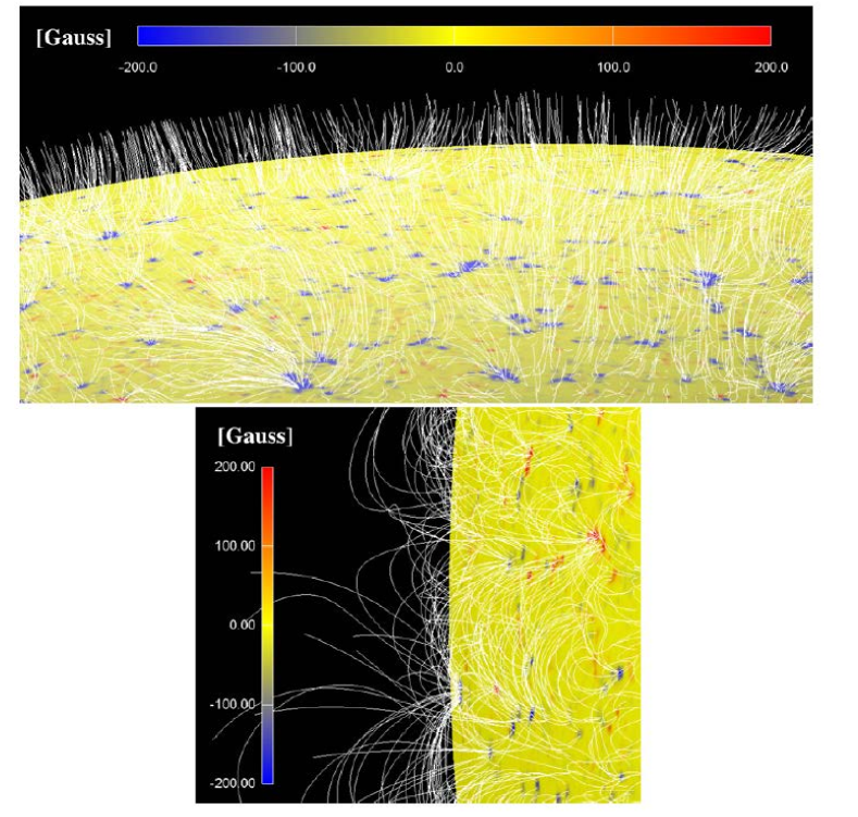
Figure 27: Selected field lines, calculated from a PFSS model, outlining the coronal magnetic field structure associated to a CH (a) around the north pole of the Sun and (b) in a quiet-Sun area near the East limb. It can be seen that the majority of field lines that originate in kG-features fan out just above the photosphere (in a canopy-like fashion) and that they are open. The color-coded surface indicates the vertical magnetic field, where blue/red represents negative/positive polarity. It is evident that the polar region is dominated by a specific (negative, in this case) polarity, while the QS represents an environment of mixed polarity. (Figure 11 from Ito et al. (2010). © AAS. Reproduced with permission.)

6.2.3 Polar plumes

Polar plumes are visible in the form of thin streamers above the solar limb in the polar regions. They have been studied intensively, e. g., by a coordinated observing campaign (SOHO and several of other space-borne and ground-based instruments; see Deforest et al., 1997). A comprehensive review was given by Wilhelm et al. (2011), including discussion of the 3D structure of polar plumes, details of their generation and of their interaction with the solar wind. Here, we concentrate on the magnetic field structure of polar plumes.

Supported by potential field models, polar plumes are associated to open fields on large scales (Suess, 1982). While the source region of these plumes is usually not visible in coronal EUV images, stereoscopic reconstructions by Feng et al. (2009) showed that they connected to photospheric magnetic patches. Wang and Sheeley (1995) and Wang (1998) proposed that plumes are produced by the reconnection of emerging mixed polarity fields with previously existing unipolar fields. Raouafi et al. (2008) reported that most of the studied coronal jets in polar regions are generally followed by plumes. The authors pointed out the common feature shared by plumes and jets: a mixed-polarity field area where their footpoints are located. In their picture, flux emergence and subsequent opening of previously closed loops by magnetic reconnection provide the energy for jet acceleration and eventually produce the open (plume) field geometry. For $70\%$ of the observed polar jets, a plume was found to form within minutes to hours after the appearance of the jet. Such an association is plausible, given that the formation mechanism of jets is also thought to be the reconnection of emerging flux with previously present unipolar field (e. g., Yokoyama and Shibata, 1995; Canfield et al., 1996).

6.2.4 Polar Jets

Jets are ubiquitous dynamical features which occur in CHs, ARs and the QS. (For a discussion of jets occurring in the QS, see section 5.3.1.) For example, Cirtain et al. (2007) detected about 10 fast jets per hour in a PCH. Detailed analysis revealed that at least a sub-set of jets is characterized by two distinct velocities: one close to the sound speed ($\approx$ 200 km s^-1) and another one on the order of the Alfvén speed ($\approx$ 1000 km s^-1). This might be explained with the following scenario. Initially, the outflow triggered by reconnection has a velocity close to the Alfvén speed. Due to the transit of a reconnected magnetic field line to a relaxed configuration, Alfvén waves become excited, which might also contribute to the acceleration of the fast solar wind. The reconnection process also has the effect of heating the coronal plasma by converting magnetic to thermal energy. As a consequence, the plasma expands, which also leads to a plasma outflow. Its speed, however, is significantly lower (sound speed) than the outflow component caused by magnetic reconnection.

Using spectroscopic data from SOHO/SUMER and Hinode/EIS, Kamio et al. (2009) investigated the formation of jets in the transition-region and coronal environment of CHs. They deduced that the open magnetic fields associated with the jets were rooted in kG vertical fields at photospheric levels. They also found that both explosive phenomena and cool up-flows were caused by magnetic reconnection with low-lying loops in the transition region, confirming and extending earlier results. Yang et al. (2011b) investigated the boundaries of the equatorial extension of a PCH using co-observations of the photospheric magnetic field from SDO/HMI and the coronal plasma EUV emission with SDO/AIA. A number of jets were recognized in the EUV images and interpreted as signatures of magnetic reconnection. The latter was supported by co-temporal emergence and cancellation of magnetic flux seen in the photospheric magnetic field data. The coexistence of open and closed fields at CH boundaries naturally result in energy deposition by multiple reconnection events, those thought to produce jets.

6.2.5 Contribution to the solar wind

Tian et al. (2011) observed high-speed outflows of $\approx 120$ km s^-1 in plume-like structures in polar and ECHs, as well as quiet-Sun regions in SDO/AIA images. Comparison with a potential coronal magnetic field model based on SDO/HMI measurements led the authors to conclude that plume-related jets do not necessarily contribute to the solar wind. This confirmed what was found earlier by Feng et al. (2009) using STEREO/SECCHI data, namely that the contribution of polar plumes to the fast solar wind is insignificant. Note, however, that studies of outflows in polar plumes and inter-plume-regions are contradictory. For instance, Gabriel et al. (2003) claimed that about half of the fast solar wind at a distance of 1.1 solar radii originates from plumes. A corresponding discussion is beyond the scope of this work and we refer to section 4 of Wilhelm et al. (2011) for a detailed review of the relevant literature.

6.3 Equatorial coronal holes

During cycle phases of higher solar activity, CHs are present at all latitudes. ECHs are smaller and persist for a shorter time than PCHs. Nevertheless they persist over several solar rotations. Many low-latitude holes are located close to the edges of ARs. That helps to understand the changes of CHs in the course of the solar cycle: because ARs tend to emerge closer and closer to the solar equator, CHs exhibit a similar trend. In some cases ARs appear even within these CHs (see section 3 in Cranmer, 2009, for details). As a consequence of the emerging AR, the CH decreases in size.

6.3.1 Formation and evolution

In contrast to the differential character of the solar rotation in the sub-surface layers of the Sun ECHs at coronal heights rotate more rigidly (Timothy et al., 1975), but still with a differential character (Insley et al., 1995). Glencross (1974) suggested “magnetic merging”, or more precisely magnetic reconnection, of oppositely directed magnetic arches could possibly form CHs and also explain their more rigid rotation.

Associated numerical experiments have been carried out by Wang et al. (1996) and as a possible origin of ECHs, the interaction of bipolar ARs has been identified, which is able to explain the imbalance of magnetic flux that is characteristic for CHs. Modelling a bipolar magnetic region superposed on an axisymmetric dipole global field, Wang et al. (1996) found that both, the local photospheric field as well as the overlying global coronal field, determine the location of open field regions. The rotation of the CH, however, is then controlled by the bipolar magnetic region with which it co-rotates (see Figure 28). During this process the coronal magnetic field has to change its topology by magnetic reconnection from closed to open, and vice versa when entering and leaving the CH. By definition, magnetic reconnection is prohibited in potential field models, as is the breaking down of the frozen-in condition of the high-conductivity coronal plasma.

Therefore, physically more advanced approaches, able to investigate the nature of the magnetic reconnection involved in the development of CHs, were carried out by Lionello et al. (2005). They found that while the magnetic structure of a CH might be relatively stable, magnetic flux may permanently move in or out of the region covered by the CH, causing reconnection to happen. The transitions from closed to open magnetic fields at the boundaries of CHs were suspected to be the origin of the slow (with velocities of $\lesssim 450$ km s^-1) solar wind (Wang et al., 1996). Interchange reconnection between open and closed fields at the boundary of CHs are thought to be responsible for, or at least related to coronal jets and polar plumes.

Recently, Petrie and Haislmaier (2013) used synoptic magnetograms from GONG to approximate the corona with a potential-field model and compared it to synoptic EUV maps from STEREO. They investigated the relationship between decaying ARs and CHs at low latitudes. Newly emerging ARs generally result in significant changes of the global coronal magnetic-field structure and cause the re-shaping of the streamer belt. Decaying ARs which were found to evolve steadily and gradually, however, would not yield a considerable change of the global field, even though they left behind a considerable flux imbalance. The authors argued that some of the imbalanced flux, nevertheless needs to (re)connect elsewhere and thus to form the streamer belt or the open fields.

Figure 28: Examples for idealized open magnetic field regions: Panel A shows an axisymmetric dipole, panel B a bipolar magnetic region (BMR) and Panel C a superposition of dipole and BMR. Orange and green field lines originate in positive and negative flux regions, respectively. The color coding on the solar surface correspond to different regions: white and black to positive and negative polarities in ARs, yellow and light blue to positive and negative polarities in CHs, red and dark blue to positive and negative background fields. (Adapted from Figure 4 of (Wang et al., 1996). Reprinted with permission from AAAS.)

6.3.2 Comparison with quiet-Sun magnetic fields

The local, small-scale magnetic field structure of ECHs in the upper solar atmosphere has been investigated by Wiegelmann and Solanki (2004) under the presumption that electromagnetic radiation from coronal plasma mainly originates from closed magnetic loops, while open field lines remain almost invisible owing to their strongly reduced plasma density. A statistical study using a potential field model based on SOHO/MDI magnetograms revealed that only small closed magnetic loops exist within the CH. The apex of these loops does not reach coronal heights. Above a certain height, all field lines were found to be open since the minority flux has been cancelled out. In contrast, quiet-Sun areas are more or less flux-balanced and thus contain field lines of various apex heights, including numerous field lines reaching up into the corona (see Figure 29). For corresponding investigations of PCHs see section 6.2.2 and Figure 27. Yang et al. (2011a) compared the magnetic field vector field in two ECHs and the QS using Hinode/SOT-SP data. They found that horizontal magnetic fields, inclination angels as well as the current density and current helicity are stronger in CHs than in the QS. The authors also concluded that the magnetic field in both QS and CH is non-potential (see also section 5.2.5).

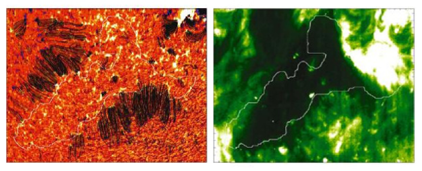
Figure 29: (a) SOHO/MDI magnetogram and overlaid closed magnetic field lines (black) obtained from a potential field model. Only closed field lines with a field strength of $\geq$ 20 G are shown. One can see that outside of the CH boundary, the number of of closed loops is significantly higher and that these loops are also longer. (b) Co-spatial EUV image from SOHO/EIT at 195 Å. The boundary of an ECH is outlined by a white contour in both images. The CH area is seen as a region of reduced emissivity. (Adapted from Figure 3 of (Wiegelmann and Solanki, 2004). With kind permission from Springer Science and Business Media.)

6.3.3 Contribution to the solar wind

Hassler et al. (1999), using Doppler maps from SOHO/SUMER, investigated the relationship between the chromospheric magnetic network and plasma outflows. They showed that the solar wind is rooted at the boundaries of the cells of the magnetic network. Tu et al. (2005) went a step further and combined data from the same instrument with a potential coronal magnetic field model based on SOHO/MDI data. A correlation analysis of the modelled field structure, of observed Doppler-velocity and radiance maps revealed an acceleration of the solar wind at heights between five and 20 Mm above the Sun’s surface, and originating from coronal funnels (Figure 30). Jin and Wang (2011), using Hinode/SOT-SP data were able to support the scenario described by Tu et al. (2005), namely that the solar wind streams along magnetic funnels and the magnetic reconnection of open and closed fields might provide energy for the acceleration of the particles.

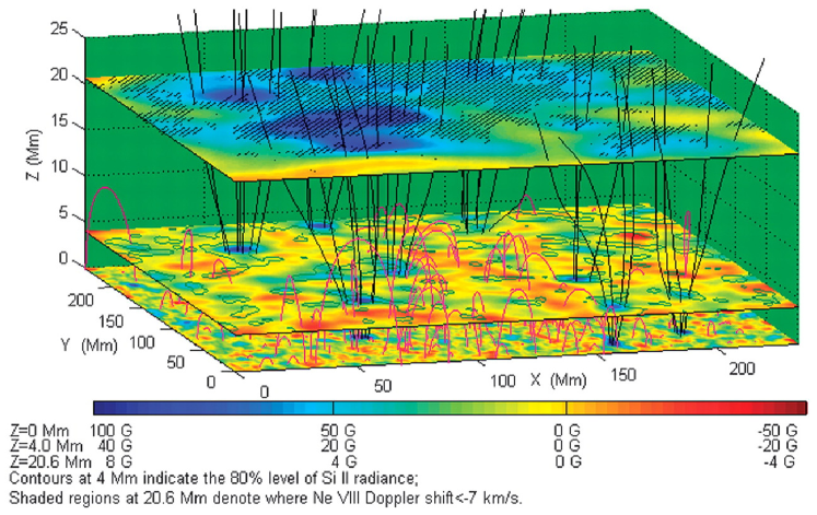
Figure 30: The linear force-free coronal magnetic field model shows open (black) and closed (red) field lines. Because of the decreasing magnetic field strength, the inserted magnetic maps at 0 Mm, 4 Mm and 20.6 Mm correspond to a different color bar. At the 4 Mm and 20.6 Mm level the authors made a correlation analysis of the extrapolated magnetic field Bz and Doppler maps from SOHO/SUMER. The shaded area at 20.6 Mm corresponds to a detected outflow faster than 7 km s^-1. (Figure 5 of Tu et al. 2005. Reprinted with permission from AAAS.)

7 Conclusion and Outlook

Within this paper, we aimed to review our current understanding of the role of magnetic fields for the physics of the solar atmosphere, in particular the corona. In the past years, ground-based and space-borne instruments have delivered data of unprecedented spatial and temporal resolution. Together with the ever increasing sophistication of numerical techniques, this led to new insights into the nature and the dynamic evolution of the coronal magnetic field. A broad range of spatial scales is involved in coronal processes: from very small scales, at which magnetic reconnection may locally reconfigure the magnetic field, to very large scales, at which the long-term recycling of the global magnetic field takes place.

There are a number of techniques available for the measurement of the coronal magnetic field, but none has found widespread and regular use. Observations at radio wavelengths have provided by far the most direct measurements of coronal magnetic fields, augmented by polarization measurements in coronal lines in the infrared for a relatively small number of cases. More frequent are observations using magnetically sensitive chromospheric lines in the infrared, which can sample layers close to the coronal base. Current limitations on the spatial and temporal resolution at radio frequencies are expected to be partly lifted once FASR starts operating. More regular observations of the coronal magnetic field vector are also envisaged with the NSO/DKIST telescope. A more indirect approach is taken by coronal seismology, which permits the magnetic field strength to be derived from the analysis of oscillating loops.

Nevertheless, by far the most accurate routine measurements are of the magnetic field in the photosphere, ranging from global scales with SDO to high resolution measurements with Sunrise.

The instabilities that might trigger magnetic reconnection are still only accessible through 3D numerical MHD models. This is also because even the present imaging and spectropolarimetric instrumentation with the highest spatial resolution (e. g., Sunrise and Hi-C), might still be far from resolving the relevant spatial scales. Besides, high spatial resolution often comes with a restricted FOV. Such restrictions are less severe for the analysis of processes observed on larger active-region scales. Coronal imaging data of sufficiently high spatial resolution and temporal cadence, in the form of SDO/AIA images, have allowed detailed analysis of the coronal dynamics in recent years. The interpretation of these observations has been increasingly aided by static force-free magnetic field models which, at the same time, were validated by the match with structures seen in the same coronal images. The force-free modelling approach is well justified in the corona above an active region owing to the low plasma $\beta$ there, but less suitable to model the quiet Sun, where $\beta$ is not low and non-magnetic forces have to be taken into account, e.g., with magneto-static and MHD-models.

For studying the evolution of coronal magnetic fields a strong tool is the combination of flux-transport models and extrapolation techniques. Complementary stereoscopic and tomographic methods significantly improved the ability to reconstruct the 3D structure of coronal loops by using simultaneously observed 2D images from a number of vantage points, such as SOHO/EIT, the STEREO spacecrafts, SDO/AIA, and in the future also Solar Orbiter.

A promising approach is to combine extrapolations from photospheric fields and stereoscopy within one model. Such attempts are still in their infancy though and currently non-linear force-free extrapolations of the photospheric field vector into the corona are the state-of-the-art. The maturing of such modelling tools for the interpretation of coronal dynamics has mainly become possible due to the development and operation of advanced instruments, such as SOLIS/VSM, Hinode/SOT-SP and SDO/HMI that deliver vector magnetic field maps regularly for the entire solar disk and active-region scans with both high time cadence and high spatial resolution. In addition, forward MHS and MHD modelling techniques proved their strength in the ability to compute synthetic spectra characteristic of ARs which quantitatively reproduced spectra recorded with, e. g., SOHO/SUMER. Recent milestones using one or the other tools individually or combination with each other, were discussed throughout this review. Besides having shed light on some of the hidden dynamics of the magnetic field, indirectly accessible to us only by the analysis of coronal images, the scientific outcome in recent years naturally also changed the course of the field and uncovered and/or strengthened the importance of answering still open questions.

On small granulation scales, the permanent restructuring of line-tied, braided and/or twisted active-region magnetic fields has been a strong contender for providing a contribution to the heating of the coronal plasma to the observed temperatures. Its contribution to the release of parts of the vast amount of energy stored in the coronal active-region magnetic fields, however, is still to be determined in detail. On active-region scales, dynamic phenomena such as flares and CMEs received great attention and have revealed some of their secrets. We are increasingly able to relate observed flare-associated energetics to specific magnetic field structures, both in space and in time. The ability to predict eruptive phenomena, however, is still in its infancy. Detailed analysis of the eruption-associated magnetic field topology and its evolution is highlighting the complex interplay between photospheric driver and coronal response, underlining that the task of attempting any forecasting is a challenging one. Similarly demanding is the prediction of the long-term behaviour of activity and even more so since the importance of local eruptive processes for the cyclic global restructuring remains unclear.

Finally, the findings of recent years showed us that the magnetic structure of the solar corona, even during times of low solar activity when the global magnetic field is thought to be best represented by a “simple” dipole field, is rather complex. Consequently, much work is still needed to unravel the nature of the Sun’s magnetic field, on local as well as on global scales, the latter being important in order to understand its contribution to the solar wind and its effects on our interplanetary environment.

Appendix A Abbreviations

AR(s)	Active Region(s)
CH(s)	Coronal Hole(s)
CME(s)	Coronal Mass Ejection(s)
ECH(s)	Equatorial Coronal Hole(s)
EUV	Extreme Ultraviolet)
FOV	Field-Of-View
FASR	Frequency Agile Solar Radiotelescope (Gary and Keller, 2005)
GOES	Geostationary Operational Environmental Satellite
	(http://www.goes.noaa.gov/)
Hi-C	High-resolution Coronal Imager (Golub et al., 2006; Cirtain et al., 2013)
Hinode	Solar-B (Ichimoto and Solar-B Team, 2005)
Hinode/EIS	Hinode EUV Imaging Spectrometer (Culhane et al., 2007)
Hinode/SOT	Hinode Solar Optical Telescope (Suematsu et al., 2008)
Hinode/SOT-SP	Hinode SOT Spectro-Polarimeter (Tsuneta et al., 2008b; Lites et al., 2013)
KPNO	Kitt Peak National Observatory (http://www.noao.edu/kpno/
LFF	Linear Force-Free
LOS	Line-Of-Sight
MC(s)	Magnetic Cloud(s)
MHD	Magneto-Hydro-Dynamic
M(H)S	Magneto-(Hydro-)Static
NSO	National Solar Observatory (http://www.nso.edu/)
NSO/DIKST	NSO Daniel K. Inouye Solar Telescope (http://atst.nso.edu/)
NLFF	Nonlinear Force-Free
PCH(s)	Polar Coronal Hole(s)
PIL(s)	Polarity Inversion Line(s)
PFSS	Potential Field Source Surface
QSL(s)	Quasi-Separatrix Layer(s)
QS	Quiet Sun
SDO	Solar Dynamics Observatory (Pesnell et al., 2012)
SDO/AIA	SDO Atmospheric Imaging Assembly (Lemen et al., 2012)
SDO/HMI	SDO Helioseismic and Magnetic Imager (Schou et al., 2012)
SOHO	Solar and Heliospheric Observatory (Scherrer et al., 1995)
SOHO/EIT	SOHO Extreme ultraviolet Imaging Telescope (Delaboudiniére et al. 1995)
SOHO/LASCO	SOHO Large Angle and Spectrometric Coronagraph (Brueckner et al., 1995)
SOHO/MDI	SOHO Michelson Doppler Imager (Scherrer et al., 1995)
SOHO/SUMER	SOHO Solar Ultraviolet Measurements of Emitted Radiation
	(Wilhelm et al., 1995)
SOLIS	Solar Optical Long-term Investigations of the Sun (Keller et al., 2003a)
SOLIS/VSM	SOLIS Vector SpectroMagnetograph (Keller et al., 2003b)
Solar Orbiter	(Müller et al., 2013)
STEREO	Solar-TErrestrial RElations Observatory (Kaiser et al., 2008)
STEREO/SECCHI	STEREO Sun Earth Connection Coronal and Heliospheric Investigation
	(Howard et al., 2002)
STEREO/SECCHI-COR1(2)	STEREO/SECCHI inner (outer) CORonograph (Liu et al., 2009b)
STEREO/SECCHI-EUVI	STEREO/SECCHI Extreme UltraViolet Imager (Wuelser et al., 2004)
Sunrise	Solar-C (Solanki et al., 2010; Barthol et al., 2011)
SXR(s)	Soft X-ray(s)
Sunrise/IMaX	Sunrise Imaging Magnetograph eXperiment (Martínez Pillet et al. 2011)
TEL(s)	Trans-Equatorial Loop(s)
TRACE	Transition Region and Coronal Explorer (Handy et al., 1999)
VTT	Vacuum Tower Telescope http://www.kis.uni-freiburg.de/
WIND/WAVES	(Bougeret et al., 1995)
Yohkoh	Solar-A (Tsuneta et al., 1991)
Yohkoh/SXT	Yohkoh Soft X-ray Telescope (Tsuneta et al., 1991)

References

- Abramenko and Longcope (2005) V. I. Abramenko and D. W. Longcope. Distribution of the Magnetic Flux in Elements of the Magnetic Field in Active Regions. Astrophys. J., 619:1160–1166, Feb. 2005. doi: 10.1086/426710.
- Abramenko et al. (2011) V. I. Abramenko, V. Carbone, V. Yurchyshyn, P. R. Goode, R. F. Stein, F. Lepreti, V. Capparelli, and A. Vecchio. Turbulent Diffusion in the Photosphere as Derived from Photospheric Bright Point Motion. Astrophys. J., 743:133, Dec. 2011. doi: 10.1088/0004-637X/743/2/133.
- Aly (1989) J. J. Aly. On the reconstruction of the nonlinear force-free coronal magnetic field from boundary data. Sol. Phys., 120:19–48, Mar. 1989.
- Antiochos and DeVore (1999) S. K. Antiochos and C. R. DeVore. The Role of Helicity in Magnetic Reconnection: 3D Numerical Simulations. Washington DC American Geophys. Union Geophys. Mon. Ser., 111:187, 1999.
- Arnaud (1982a) J. Arnaud. Observed polarization of the Fe XIV 5303 coronal emission line. Astron. Astrophys., 112:350–354, Aug. 1982a.
- Arnaud (1982b) J. Arnaud. The analysis of Fe XIV 5303 coronal emission-line polarization measurements. Astron. Astrophys., 116:248–254, Dec. 1982b.
- Aschwanden (2005) M. J. Aschwanden. Physics of the Solar Corona. An Introduction with Problems and Solutions (2nd edition). Chichester: Praxis Publishing Ltd., Dec. 2005.
- Aschwanden (2011) M. J. Aschwanden. Solar Stereoscopy and Tomography. Living Rev. Sol. Phys., 8:5, Oct. 2011. doi: 10.12942/lrsp-2011-5.
- Aschwanden and Boerner (2011) M. J. Aschwanden and P. Boerner. Solar Corona Loop Studies with the Atmospheric Imaging Assembly. I. Cross-sectional Temperature Structure. Astrophys. J., 732:81, May 2011. doi: 10.1088/0004-637X/732/2/81.
- Aschwanden et al. (2014) M. J. Aschwanden, X. Sun, and Y. Liu. The Magnetic Field of Active Region 11158 during the 2011 February 12-17 Flares: Differences between Photospheric Extrapolation and Coronal Forward-Fitting Methods. Astrophys. J., 785:34, Apr. 2014. doi: 10.1088/0004-637X/785/1/34.
- Athay et al. (1983) R. G. Athay, C. W. Querfeld, R. N. Smartt, E. Landi Degl’Innocenti, and V. Bommier. Vector magnetic fields in prominences. III - HeI D3 Stokes profile analysis for quiescent and eruptive prominences. Sol. Phys., 89:3–30, Nov. 1983. doi: 10.1007/BF00211948.
- Aulanier et al. (2000) G. Aulanier, E. E. DeLuca, S. K. Antiochos, R. A. McMullen, and L. Golub. The Topology and Evolution of the Bastille Day Flare. Astrophys. J., 540:1126–1142, Sept. 2000. doi: 10.1086/309376.
- Aulanier et al. (2005) G. Aulanier, E. Pariat, and P. Démoulin. Current sheet formation in quasi-separatrix layers and hyperbolic flux tubes. Astron. Astrophys., 444:961–976, Dec. 2005. doi: 10.1051/0004-6361:20053600.
- Bai (2003) T. Bai. Periodicities in Solar Flare Occurrence: Analysis of Cycles 19-23. Astrophys. J., 591:406–415, July 2003. doi: 10.1086/375295.
- Baker et al. (2009) D. Baker, L. van Driel-Gesztelyi, C. H. Mandrini, P. Démoulin, and M. J. Murray. Magnetic Reconnection along Quasi-separatrix Layers as a Driver of Ubiquitous Active Region Outflows. Astrophys. J., 705:926–935, Nov. 2009. doi: 10.1088/0004-637X/705/1/926.
- Bao et al. (2002) S. D. Bao, T. Sakurai, and Y. Suematsu. The sources of magnetic field twist in solar active regions. Astrophys. J., 573:445–453, July 2002.
- Barthol et al. (2011) P. Barthol, A. Gandorfer, S. K. Solanki, M. Schüssler, B. Chares, W. Curdt, W. Deutsch, A. Feller, D. Germerott, B. Grauf, K. Heerlein, J. Hirzberger, M. Kolleck, R. Meller, R. Müller, T. L. Riethmüller, G. Tomasch, M. Knölker, B. W. Lites, G. Card, D. Elmore, J. Fox, A. Lecinski, P. Nelson, R. Summers, A. Watt, V. Martínez Pillet, J. A. Bonet, W. Schmidt, T. Berkefeld, A. M. Title, V. Domingo, J. L. Gasent Blesa, J. C. Del Toro Iniesta, A. López Jiménez, A. Álvarez-Herrero, L. Sabau-Graziati, C. Widani, P. Haberler, K. Härtel, D. Kampf, T. Levin, I. Pérez Grande, A. Sanz-Andrés, and E. Schmidt. The Sunrise Mission. Sol. Phys., 268:1–34, Jan. 2011. doi: 10.1007/s11207-010-9662-9.
- Baty and Heyvaerts (1996) H. Baty and J. Heyvaerts. Electric current concentration and kink instability in line-tied coronal loops. Astron. Astrophys., 308:935–950, Apr. 1996.
- Baumann et al. (2004) I. Baumann, D. Schmitt, M. Schüssler, and S. K. Solanki. Evolution of the large-scale magnetic field on the solar surface: A parameter study. Astron. Astrophys., 426:1075–1091, Nov. 2004. doi: 10.1051/0004-6361:20048024.
- Beck et al. (2014) C. Beck, D. P. Choudhary, and R. Rezaei. A Three-dimensional View of the Thermal Structure in a Super-penumbral Canopy. Astrophys. J., 788:183, June 2014. doi: 10.1088/0004-637X/788/2/183.
- Bellan (1999) P. M. Bellan. Magnetic helicity and relaxation: Theory. In M. R. Brown, R. C. Canfield, and A. A. Pevtsov, editors, Helicity in space and laboratory plasmas, pages 119–128, 1999.
- Bellan (2006) P. M. Bellan. Fundamentals of plasma physics. Cambridge: Cambridge University Press, Jan. 2006.
- Benz (2008) A. O. Benz. Flare Observations. Living Rev. Sol. Phys., 5(1), 2008. URL http://www.livingreviews.org/lrsp-2008-1.
- Berdyugina and Usoskin (2003) S. V. Berdyugina and I. G. Usoskin. Active longitudes in sunspot activity: Century scale persistence. Astron. Astrophys., 405:1121–1128, July 2003. doi: 10.1051/0004-6361:20030748.
- Berger (1984) M. A. Berger. Rigorous new limits on magnetic helicity dissipation in the solar corona. Geophys. Astrophys. Fluid Dyn., 30:79–104, Sept. 1984.
- Berger and Asgari-Targhi (2009) M. A. Berger and M. Asgari-Targhi. Self-organized Braiding and the Structure of Coronal Loops. Astrophys. J., 705:347–355, Nov. 2009. doi: 10.1088/0004-637X/705/1/347.
- Berger and Ruzmaikin (2000) M. A. Berger and A. Ruzmaikin. Rate of helicity production by solar rotation. J. Geophys. Res., 105:10,481–10,490, May 2000. doi: 10.1029/1999JA900392.
- Berger and Title (1996) T. E. Berger and A. M. Title. On the Dynamics of Small-Scale Solar Magnetic Elements. Astrophys. J., 463:365, May 1996. doi: 10.1086/177250.
- Bernasconi et al. (2005) P. N. Bernasconi, D. M. Rust, and D. Hakim. Advanced Automated Solar Filament Detection And Characterization Code: Description, Performance, And Results. Sol. Phys., 228:97–117, May 2005. doi: 10.1007/s11207-005-2766-y.
- Berton and Sakurai (1985) R. Berton and T. Sakurai. Stereoscopic determination of the three-dimensional geometry of coronal magnetic loops. Sol. Phys., 96:93–111, Mar. 1985. doi: 10.1007/BF00239795.
- Bieber and Rust (1995) J. W. Bieber and D. M. Rust. The Escape of Magnetic Flux from the Sun. Astrophys. J., 453:911, Nov. 1995. doi: 10.1086/176451.
- Bleybel et al. (2002) A. Bleybel, T. Amari, L. van Driel-Gesztelyi, and K. D. Leka. Global budget for an eruptive active region. I. Equilibrium reconstruction approach. Astron. Astrophys., 395:685–695, Nov. 2002. doi: 10.1051/0004-6361:20021332.
- Bogdan and Low (1986) T. J. Bogdan and B. C. Low. The three-dimensional structure of magnetostatic atmospheres. II - Modeling the large-scale corona. Astrophys. J., 306:271–283, July 1986. doi: 10.1086/164341.
- Bogod et al. (2012) V. M. Bogod, A. G. Stupishin, and L. V. Yasnov. On Magnetic Fields of Active Regions at Coronal Heights. Sol. Phys., 276:61–73, Feb. 2012. doi: 10.1007/s11207-011-9850-2.
- Borrero and Ichimoto (2011) J. M. Borrero and K. Ichimoto. Magnetic structure of sunspots. Living Rev. Sol. Phys., 8(4), 2011. doi: 10.12942/lrsp-2011-4. URL http://www.livingreviews.org/lrsp-2011-4.
- Bougeret et al. (1995) J.-L. Bougeret, M. L. Kaiser, P. J. Kellogg, R. Manning, K. Goetz, S. J. Monson, N. Monge, L. Friel, C. A. Meetre, C. Perche, L. Sitruk, and S. Hoang. Waves: The Radio and Plasma Wave Investigation on the Wind Spacecraft. Space Sci. Rev., 71:231–263, Feb. 1995. doi: 10.1007/BF00751331.
- Bray and Loughhead (1964) R. J. Bray and R. E. Loughhead. Sunspots. London: Chapman & Hall, 1964.
- Bray et al. (1991) R. J. Bray, L. E. Cram, C. J. Durrant, and R. E. Loughhead. Plasma loops in the solar corona. Cambridge Astrophysics Series. Cambridge: Cambridge University Press, 1991.
- Brekke et al. (1997) P. Brekke, O. Kjeldseth-Moe, N. Brynildsen, P. Maltby, S. V. H. Haugan, R. A. Harrison, W. T. Thompson, and C. D. Pike. Flows and Dynamics in the Corona Observed with the Coronal Diagnostic Spectrometer (cds). Sol. Phys., 170:163–177, 1997. doi: 10.1023/A:1004945702259.
- Briand and Solanki (1995) C. Briand and S. K. Solanki. Empirical models of solar magnetic elements: constraints imposed by MgI Stokes profiles. Astron. Astrophys., 299:596, July 1995.
- Brosius and White (2006) J. W. Brosius and S. M. White. Radio Measurements of the Height of Strong Coronal Magnetic Fields Above Sunspots at the Solar Limb. Astrophys. J. Lett., 641:L69–L72, Apr. 2006. doi: 10.1086/503774.
- Brosius et al. (1997) J. W. Brosius, J. M. Davila, R. J. Thomas, and S. M. White. Coronal Magnetography of a Solar Active Region Using Coordinated SERTS and VLA Observations. Astrophys. J., 488:488–498, Oct. 1997.
- Brown et al. (2003) D. S. Brown, R. W. Nightingale, D. Alexander, C. J. Schrijver, T. R. Metcalf, R. A. Shine, A. M. Title, and C. J. Wolfson. Observations of Rotating Sunspots from TRACE. Sol. Phys., 216:79–108, Sept. 2003.
- Brueckner and Bartoe (1983) G. E. Brueckner and J.-D. F. Bartoe. Observations of high-energy jets in the corona above the quiet sun, the heating of the corona, and the acceleration of the solar wind. Astrophys. J., 272:329–348, Sept. 1983. doi: 10.1086/161297.
- Brueckner et al. (1995) G. E. Brueckner, R. A. Howard, M. J. Koomen, C. M. Korendyke, D. J. Michels, J. D. Moses, D. G. Socker, K. P. Dere, P. L. Lamy, A. Llebaria, M. V. Bout, R. Schwenn, G. M. Simnett, D. K. Bedford, and C. J. Eyles. The Large Angle Spectroscopic Coronagraph (LASCO). Sol. Phys., 162:357–402, Dec. 1995. doi: 10.1007/BF00733434.
- Bruls and Solanki (1995) J. H. M. J. Bruls and S. K. Solanki. Infrared lines as probes of solar magnetic features. IX. MgI 12m diagnostics of solar plage. Astron. Astrophys., 293:240–251, Jan. 1995.
- Bruno and Carbone (2013) R. Bruno and V. Carbone. The solar wind as a turbulence laboratory. Living Rev. Sol. Phys., 10(2), 2013. doi: 10.12942/lrsp-2013-2. URL http://www.livingreviews.org/lrsp-2013-2.
- Buente et al. (1993) M. Buente, S. K. Solanki, and O. Steiner. Centre-to-limb variation of the Stokes V asymmetry in solar magnetic flux tubes. Astron. Astrophys., 268:736–748, Feb. 1993.
- Bühler et al. (2013) D. Bühler, A. Lagg, and S. K. Solanki. Quiet Sun magnetic fields observed by Hinode: Support for a local dynamo. Astron. Astrophys., 555:A33, July 2013. doi: 10.1051/0004-6361/201321152.
- Burlaga et al. (1981) L. Burlaga, E. Sittler, F. Mariani, and R. Schwenn. Magnetic loop behind an interplanetary shock - Voyager, Helios, and IMP 8 observations. J. Geophys. Res., 86:6673–6684, Aug. 1981. doi: 10.1029/JA086iA08p06673.
- Burlaga (1988) L. F. Burlaga. Magnetic clouds and force-free fields with constant alpha. J. Geophys. Res., 93:7217–7224, July 1988. doi: 10.1029/JA093iA07p07217.
- Caligari et al. (1995) P. Caligari, F. Moreno-Insertis, and M. Schussler. Emerging flux tubes in the solar convection zone. 1: Asymmetry, tilt, and emergence latitude. Astrophys. J., 441:886–902, Mar. 1995. doi: 10.1086/175410.
- Cameron et al. (2011) R. Cameron, A. Vögler, and M. Schüssler. Decay of a simulated mixed-polarity magnetic field in the solar surface layers. Astron. Astrophys., 533:A86, Sept. 2011. doi: 10.1051/0004-6361/201116974.
- Canfield et al. (1996) R. C. Canfield, K. P. Reardon, K. D. Leka, K. Shibata, T. Yokoyama, and M. Shimojo. H alpha Surges and X-Ray Jets in AR 7260. Astrophys. J., 464:1016, June 1996. doi: 10.1086/177389.
- Canfield et al. (1999) R. C. Canfield, H. S. Hudson, and D. E. McKenzie. Sigmoidal morphology and eruptive solar activity. Geophys. Res. Lett., 26:627–630, Mar. 1999. doi: 10.1029/1999GL900105.
- Cargill (2009) P. J. Cargill. Coronal magnetism: Difficulties and prospects. Space Sci. Rev., 144:413–421, Apr. 2009. doi: 10.1007/s11214-008-9446-9.
- Carlsson and Stein (1997) M. Carlsson and R. F. Stein. Formation of Solar Calcium H and K Bright Grains. Astrophys. J., 481:500–514, May 1997.
- Carmichael (1964) H. Carmichael. A Process for Flares. NASA Special Publication, 50:451, 1964.
- Carroll (1933) J. A. Carroll. Zones of Apparent Inhibition of sunspots on the Solar Disc. Nature, 131:548–549, Apr. 1933. doi: 10.1038/131548b0.
- Centeno et al. (2007) R. Centeno, H. Socas-Navarro, B. Lites, M. Kubo, Z. Frank, R. Shine, T. Tarbell, A. Title, K. Ichimoto, S. Tsuneta, Y. Katsukawa, Y. Suematsu, T. Shimizu, and S. Nagata. Emergence of Small-Scale Magnetic Loops in the Quiet-Sun Internetwork. Astrophys. J. Lett., 666:L137–L140, Sept. 2007. doi: 10.1086/521726.
- Chae et al. (2004) J. Chae, Y.-J. Moon, and Y.-D. Park. Determination of magnetic helicity content of solar active regions from SOHO/MDI magnetograms. Sol. Phys., 223:39–55, Sept. 2004. doi: 10.1007/s11207-004-0938-9.
- Chandra et al. (2009) R. Chandra, B. Schmieder, G. Aulanier, and J. M. Malherbe. Evidence of Magnetic Helicity in Emerging Flux and Associated Flare. Sol. Phys., 258:53–67, Aug. 2009. doi: 10.1007/s11207-009-9392-z.
- Chandra et al. (2010) R. Chandra, E. Pariat, B. Schmieder, C. H. Mandrini, and W. Uddin. How Can a Negative Magnetic Helicity Active Region Generate a Positive Helicity Magnetic Cloud? Sol. Phys., 261:127–148, Jan. 2010. doi: 10.1007/s11207-009-9470-2.
- Charbonneau (2010) P. Charbonneau. Dynamo models of the solar cycle. Living Rev. Sol. Phys., 7(3), 2010. doi: 10.12942/lrsp-2010-3. URL http://www.livingreviews.org/lrsp-2010-3.
- Chen and Wang (2012) A. Q. Chen and J. X. Wang. Quantifying solar superactive regions with vector magnetic field observations. Astron. Astrophys., 543:A49, July 2012. doi: 10.1051/0004-6361/201118037.
- Chen et al. (2011) C. Chen, Y. Wang, C. Shen, P. Ye, J. Zhang, and S. Wang. Statistical study of coronal mass ejection source locations: 2. Role of active regions in CME production. J. Geophys. Res. (Space Physics), 116(A15):A12108, Dec. 2011. doi: 10.1029/2011JA016844.
- Chen et al. (1994) J. Chen, H. Wang, H. Zirin, and G. Ai. Observations of vector magnetic fields in flaring active regions. Sol. Phys., 154:261–273, Oct. 1994. doi: 10.1007/BF00681099.
- Chen et al. (2006) J. Chen, S. Bao, and H. Zhang. A Statistical Study of Transequatorial Loops. Sol. Phys., 235:281–294, May 2006. doi: 10.1007/s11207-006-0072-y.
- Chen et al. (2010) J. Chen, H. Lundstedt, and H. Zhang. Statistical study of twist values of transequatorial loops and the relationship with flares. Adv. Space Res., 45:537–540, Feb. 2010. doi: 10.1016/j.asr.2009.10.005.
- Chen (2011) P. F. Chen. Coronal Mass Ejections: Models and Their Observational Basis. Living Rev. Sol. Phys., 8(1), 2011. URL http://www.livingreviews.org/lrsp-2011-1.
- Chesny et al. (2013) D. L. Chesny, H. M. Oluseyi, and N. B. Orange. Non-potential Fields in the Quiet Sun Network: Extreme-ultraviolet and Magnetic Footpoint Observations. Astrophys. J. Lett., 778:L17, Nov. 2013. doi: 10.1088/2041-8205/778/1/L17.
- Cheung and Isobe (2014) M. C. M. Cheung and H. Isobe. Flux Emergence (Theory). Living Rev. Sol. Phys., 11:3, July 2014. doi: 10.12942/lrsp-2014-3.
- Chidambara Aiyar (1932) P. R. Chidambara Aiyar. Two longitudinal zones of apparent inhibition of sunspots on the solar disc. Mon. Not. Roy. Astr. Soc., 93:150, Dec. 1932.
- Chitta et al. (2014) L. P. Chitta, R. Kariyappa, A. A. van Ballegooijen, E. E. DeLuca, and S. K. Solanki. Nonlinear Force-free Field Modeling of the Solar Magnetic Carpet and Comparison with SDO/HMI and Sunrise/IMaX Observations. Astrophys. J., 793:112, Oct. 2014. doi: 10.1088/0004-637X/793/2/112.
- Cho et al. (2013) K.-S. Cho, S.-H. Park, K. Marubashi, N. Gopalswamy, S. Akiyama, S. Yashiro, R.-S. Kim, and E.-K. Lim. Comparison of Helicity Signs in Interplanetary CMEs and Their Solar Source Regions. Sol. Phys., 284:105–127, May 2013. doi: 10.1007/s11207-013-0224-9.
- Choe and Cheng (2000) G. S. Choe and C. Z. Cheng. A Model of Solar Flares and Their Homologous Behavior. Astrophys. J., 541:449–467, Sept. 2000. doi: 10.1086/309415.
- Choudhary et al. (2001) D. P. Choudhary, T. Sakurai, and P. Venkatakrishnan. Chromospheric Magnetic Field of Solar Active Regions. Astrophys. J., 560:439–444, Oct. 2001. doi: 10.1086/322501.
- Choudhary et al. (2002) D. P. Choudhary, P. Venkatakrishnan, and S. Gosain. On Magnetic Flux Imbalance in Solar Active Regions. Astrophys. J., 573:851–856, July 2002. doi: 10.1086/340754.
- Cirtain et al. (2007) J. W. Cirtain, L. Golub, L. Lundquist, A. van Ballegooijen, A. Savcheva, M. Shimojo, E. DeLuca, S. Tsuneta, T. Sakao, K. Reeves, M. Weber, R. Kano, N. Narukage, and K. Shibasaki. Evidence for Alfvén Waves in Solar X-ray Jets. Science, 318:1580–1582, Dec. 2007. doi: 10.1126/science.1147050.
- Cirtain et al. (2013) J. W. Cirtain, L. Golub, A. R. Winebarger, B. de Pontieu, K. Kobayashi, R. L. Moore, R. W. Walsh, K. E. Korreck, M. Weber, P. McCauley, A. Title, S. Kuzin, and C. E. Deforest. Energy release in the solar corona from spatially resolved magnetic braids. Nature, 493:501–503, Jan. 2013. doi: 10.1038/nature11772.
- Close et al. (2004) R. M. Close, C. E. Parnell, D. W. Longcope, and E. R. Priest. Recycling of the Solar Corona’s Magnetic Field. Astrophys. J. Lett., 612:L81–L84, Sept. 2004. doi: 10.1086/424659.
- Close et al. (2005) R. M. Close, C. E. Parnell, D. W. Longcope, and E. R. Priest. Coronal Flux Recycling Times. Sol. Phys., 231:45–70, Sept. 2005. doi: 10.1007/s11207-005-6878-1.
- Cranmer (2009) S. R. Cranmer. Coronal holes. Living Rev. Sol. Phys., 6:3, Sept. 2009. URL http://www.livingreviews.org/lrsp-2009-3.
- Culhane et al. (2007) J. L. Culhane, L. K. Harra, A. M. James, K. Al-Janabi, L. J. Bradley, R. A. Chaudry, K. Rees, J. A. Tandy, P. Thomas, M. C. R. Whillock, B. Winter, G. A. Doschek, C. M. Korendyke, C. M. Brown, S. Myers, J. Mariska, J. Seely, J. Lang, B. J. Kent, B. M. Shaughnessy, P. R. Young, G. M. Simnett, C. M. Castelli, S. Mahmoud, H. Mapson-Menard, B. J. Probyn, R. J. Thomas, J. Davila, K. Dere, D. Windt, J. Shea, R. Hagood, R. Moye, H. Hara, T. Watanabe, K. Matsuzaki, T. Kosugi, V. Hansteen, and Ø. Wikstol. The EUV Imaging Spectrometer for Hinode. Sol. Phys., 243:19–61, June 2007. doi: 10.1007/s01007-007-0293-1.
- Danilovic et al. (2010a) S. Danilovic, B. Beeck, A. Pietarila, M. Schüssler, S. K. Solanki, V. Martínez Pillet, J. A. Bonet, J. C. del Toro Iniesta, V. Domingo, P. Barthol, T. Berkefeld, A. Gandorfer, M. Knölker, W. Schmidt, and A. M. Title. Transverse Component of the Magnetic Field in the Solar Photosphere Observed by SUNRISE. Astrophys. J. Lett., 723:L149–L153, Nov. 2010a. doi: 10.1088/2041-8205/723/2/L149.
- Danilovic et al. (2010b) S. Danilovic, M. Schüssler, and S. K. Solanki. Probing quiet Sun magnetism using MURaM simulations and Hinode/SP results: support for a local dynamo. Astron. Astrophys., 513:A1, Apr. 2010b. doi: 10.1051/0004-6361/200913379.
- Dasi-Espuig et al. (2010) M. Dasi-Espuig, S. K. Solanki, N. A. Krivova, R. Cameron, and T. Peñuela. Sunspot group tilt angles and the strength of the solar cycle. Astron. Astrophys., 518:A7, July 2010. doi: 10.1051/0004-6361/201014301.
- Davila (1994) J. M. Davila. Solar Tomography. Astrophys. J., 423:871, Mar. 1994. doi: 10.1086/173864.
- de la Cruz Rodríguez and Socas-Navarro (2011) J. de la Cruz Rodríguez and H. Socas-Navarro. Are solar chromospheric fibrils tracing the magnetic field? Astron. Astrophys., 527:L8, Mar. 2011. doi: 10.1051/0004-6361/201016018.
- De Pontieu et al. (2007) B. De Pontieu, S. W. McIntosh, M. Carlsson, V. H. Hansteen, T. D. Tarbell, C. J. Schrijver, A. M. Title, R. A. Shine, S. Tsuneta, Y. Katsukawa, K. Ichimoto, Y. Suematsu, T. Shimizu, and S. Nagata. Chromospheric Alfvénic Waves Strong Enough to Power the Solar Wind. Science, 318:1574–1577, Dec. 2007. doi: 10.1126/science.1151747.
- De Rosa et al. (2009) M. L. De Rosa, C. J. Schrijver, G. Barnes, K. D. Leka, B. W. Lites, M. J. Aschwanden, T. Amari, A. Canou, J. M. McTiernan, S. Régnier, J. K. Thalmann, G. Valori, M. S. Wheatland, T. Wiegelmann, M. C. M. Cheung, P. A. Conlon, M. Fuhrmann, B. Inhester, and T. Tadesse. A Critical Assessment of Nonlinear Force-Free Field Modeling of the Solar Corona for Active Region 10953. Astrophys. J., 696:1780–1791, May 2009. doi: 10.1088/0004-637X/696/2/1780.
- de Wijn et al. (2009) A. G. de Wijn, J. O. Stenflo, S. K. Solanki, and S. Tsuneta. Small-Scale Solar Magnetic Fields. Space Sci. Rev., 144:275–315, Apr. 2009. doi: 10.1007/s11214-008-9473-6.
- DeForest (2007) C. E. DeForest. On the Size of Structures in the Solar Corona. Astrophys. J., 661:532–542, May 2007. doi: 10.1086/515561.
- Deforest et al. (1997) C. E. Deforest, J. T. Hoeksema, J. B. Gurman, B. J. Thompson, S. P. Plunkett, R. Howard, R. C. Harrison, and D. M. Hassler. Polar Plume Anatomy: Results of a Coordinated Observation. Sol. Phys., 175:393–410, Oct. 1997. doi: 10.1023/A:1004955223306.
- Del Zanna and Bromage (1999) G. Del Zanna and B. J. I. Bromage. The Elephant’s Trunk: Spectroscopic diagnostics applied to SOHO/CDS observations of the August 1996 equatorial coronal hole. J. Geophys. Res., 104:9753–9766, May 1999. doi: 10.1029/1998JA900067.
- Del Zanna and Mason (2003) G. Del Zanna and H. E. Mason. Solar active regions: SOHO/CDS and TRACE observations of quiescent coronal loops. Astron. Astrophys., 406:1089–1103, Aug. 2003. doi: 10.1051/0004-6361:20030791.
- Démoulin (2006) P. Démoulin. Extending the concept of separatrices to QSLs for magnetic reconnection. Adv. Space Res., 37:1269–1282, 2006. doi: 10.1016/j.asr.2005.03.085.
- Démoulin (2007) P. Démoulin. Recent theoretical and observational developments in magnetic helicity studies. Adv. Space Res., 39:1674–1693, 2007. doi: 10.1016/j.asr.2006.12.037.
- Démoulin and Berger (2003) P. Démoulin and M. A. Berger. Magnetic Energy and Helicity Fluxes at the Photospheric Level. Sol. Phys., 215:203–215, Aug. 2003.
- Démoulin and Pariat (2009) P. Démoulin and E. Pariat. Modelling and observations of photospheric magnetic helicity. Adv. Space Res., 43:1013–1031, Apr. 2009. doi: 10.1016/j.asr.2008.12.004.
- Demoulin et al. (1997) P. Demoulin, L. G. Bagala, C. H. Mandrini, J. C. Henoux, and M. G. Rovira. Quasi-separatrix layers in solar flares. II. Observed magnetic configurations. Astron. Astrophys., 325:305–317, Sept. 1997.
- Démoulin et al. (2002) P. Démoulin, C. H. Mandrini, L. Van Driel-Gesztelyi, M. C. Lopez Fuentes, and G. Aulanier. The Magnetic Helicity Injected by Shearing Motions. Sol. Phys., 207:87–110, May 2002.
- DeVore (2000) C. R. DeVore. Magnetic helicity generation by solar differential rotation. Astrophys. J., 539:944–953, Aug. 2000. doi: 10.1086/309274.
- Dowdy et al. (1986) J. F. Dowdy, Jr., D. Rabin, and R. L. Moore. On the magnetic structure of the quiet transition region. Sol. Phys., 105:35–45, May 1986. doi: 10.1007/BF00156374.
- Dun et al. (2007) J. Dun, H. Kurokawa, T. T. Ishii, Y. Liu, and H. Zhang. Evolution of Magnetic Nonpotentiality in NOAA AR 10486. Astrophys. J., 657:577–591, Mar. 2007. doi: 10.1086/510373.
- Durrant (1988) C. J. Durrant. The atmosphere of the sun. Bristol: Hilger, 1988.
- Durrant and McCloughan (2004) C. J. Durrant and J. McCloughan. A method of evolving synoptic maps of the solar magnetic field, II. Comparison with observations of the polar fields. Sol. Phys., 219:55–78, Jan. 2004. doi: 10.1023/B:SOLA.0000021830.88336.86.
- Einaudi and van Hoven (1983) G. Einaudi and G. van Hoven. The stability of coronal loops - Finite-length and pressure-profile limits. Sol. Phys., 88:163–177, Oct. 1983. doi: 10.1007/BF00196185.
- Evershed (1909) J. Evershed. Radial movement in sun-spots. Mon. Not. Roy. Astr. Soc., 69:454, Mar. 1909.
- Fan and Gibson (2003) Y. Fan and S. E. Gibson. The Emergence of a Twisted Magnetic Flux Tube into a Preexisting Coronal Arcade. Astrophys. J. Lett., 589:L105–L108, June 2003. doi: 10.1086/375834.
- Feng et al. (2007) L. Feng, B. Inhester, S. K. Solanki, T. Wiegelmann, B. Podlipnik, R. A. Howard, and J.-P. Wuelser. First Stereoscopic Coronal Loop Reconstructions from STEREO SECCHI Images. Astrophys. J. Lett., 671:L205–L208, Dec. 2007. doi: 10.1086/525525.
- Feng et al. (2009) L. Feng, B. Inhester, S. K. Solanki, K. Wilhelm, T. Wiegelmann, B. Podlipnik, R. A. Howard, S. P. Plunkett, J. P. Wuelser, and W. Q. Gan. Stereoscopic Polar Plume Reconstructions from STEREO/SECCHI Images. Astrophys. J., 700:292–301, July 2009. doi: 10.1088/0004-637X/700/1/292.
- Feng et al. (2013) L. Feng, T. Wiegelmann, Y. Su, B. Inhester, Y. P. Li, X. D. Sun, and W. Q. Gan. Magnetic Energy Partition between the Coronal Mass Ejection and Flare from AR 11283. Astrophys. J., 765:37, Mar. 2013. doi: 10.1088/0004-637X/765/1/37.
- Fletcher et al. (2011) L. Fletcher, B. R. Dennis, H. S. Hudson, S. Krucker, K. Phillips, A. Veronig, M. Battaglia, L. Bone, A. Caspi, Q. Chen, P. Gallagher, P. T. Grigis, H. Ji, W. Liu, R. O. Milligan, and M. Temmer. An Observational Overview of Solar Flares. Space Sci. Rev., 159:19–106, Sept. 2011. doi: 10.1007/s11214-010-9701-8.
- Floyd et al. (2014) O. Floyd, P. Lamy, and A. Llebaria. The Interaction Between Coronal Mass Ejections and Streamers: A Statistical View over 15 Years (1996 - 2010). Sol. Phys., 289:1313–1339, Apr. 2014. doi: 10.1007/s11207-013-0379-4.
- Forbes (2000) T. G. Forbes. A review on the genesis of coronal mass ejections. J. Geophys. Res., 105:23153–23166, Oct. 2000. doi: 10.1029/2000JA000005.
- Forbes et al. (2006) T. G. Forbes, J. A. Linker, J. Chen, C. Cid, J. Kóta, M. A. Lee, G. Mann, Z. Mikić, M. S. Potgieter, J. M. Schmidt, G. L. Siscoe, R. Vainio, S. K. Antiochos, and P. Riley. CME theory and models. Space Sci. Rev., 123:251–302, Mar. 2006. doi: 10.1007/s11214-006-9019-8.
- Foukal (2004) P. Foukal. Solar astrophysics; 2nd rev. ed. Wiley&Sons, 2004.
- Gabriel (1976) A. H. Gabriel. A magnetic model of the solar transition region. Phil. Trans. Roy. Soc. Lond. A, 281:339–352, May 1976.
- Gabriel et al. (2003) A. H. Gabriel, F. Bely-Dubau, and P. Lemaire. The Contribution of Polar Plumes to the Fast Solar Wind. Astrophys. J., 589:623–634, May 2003. doi: 10.1086/374416.
- Gaizauskas (1985) V. Gaizauskas. Observations of the fine structure of the chromosphere. In B. W. Lites, editor, Chromospheric Diagnostics and Modelling, pages 25–49, 1985.
- Gary and Keller (2005) D. E. Gary and C. U. Keller. Solar and Space Weather Radiophysics: Current Status and Future Developments. Astrophysics and Space Science Library. Springer, Dordrecht, 2005.
- Gary (2001) G. A. Gary. Plasma-beta above a solar active region: Rethinking the paradigm. Sol. Phys., 203:71–86, Oct. 2001.
- Gary et al. (1987) G. A. Gary, R. L. Moore, M. J. Hagyard, and B. M. Haisch. Nonpotential features observed in the magnetic field of an active region. Astrophys. J., 314:782–794, Mar. 1987. doi: 10.1086/165104.
- Georgoulis et al. (2009) M. K. Georgoulis, D. M. Rust, A. A. Pevtsov, P. N. Bernasconi, and K. M. Kuzanyan. Solar Magnetic Helicity Injected into the Heliosphere: Magnitude, Balance, and Periodicities Over Solar Cycle 23. Astrophys. J. Lett., 705:L48–L52, Nov. 2009. doi: 10.1088/0004-637X/705/1/L48.
- Gibson et al. (2004) S. E. Gibson, Y. Fan, C. Mandrini, G. Fisher, and P. Demoulin. Observational Consequences of a Magnetic Flux Rope Emerging into the Corona. Astrophys. J., 617:600–613, Dec. 2004. doi: 10.1086/425294.
- Gilchrist et al. (2012) S. A. Gilchrist, M. S. Wheatland, and K. D. Leka. The Free Energy of NOAA Solar Active Region AR 11029. Sol. Phys., 276:133–160, Feb. 2012. doi: 10.1007/s11207-011-9878-3.
- Giovanelli (1980) R. G. Giovanelli. An exploratory two-dimensional study of the coarse structure of network magnetic fields. Sol. Phys., 68:49–69, Nov. 1980. doi: 10.1007/BF00153266.
- Giovanelli and Jones (1982) R. G. Giovanelli and H. P. Jones. The three-dimensional structure of atmospheric magnetic fields in two active regions. Sol. Phys., 79:267–278, Aug. 1982. doi: 10.1007/BF00146244.
- Glencross (1974) W. M. Glencross. Formation of holes in the solar corona. Nature, 250:717–719, Aug. 1974. doi: 10.1038/250717a0.
- Golub et al. (1974) L. Golub, A. S. Krieger, J. K. Silk, A. F. Timothy, and G. S. Vaiana. Solar X-Ray Bright Points. Astrophys. J. Lett., 189:L93, Apr. 1974. doi: 10.1086/181472.
- Golub et al. (1977) L. Golub, A. S. Krieger, J. W. Harvey, and G. S. Vaiana. Magnetic properties of X-ray bright points. Sol. Phys., 53:111–121, July 1977. doi: 10.1007/BF02260212.
- Golub et al. (2006) L. Golub, J. Cirtain, E. DeLuca, G. Nystrom, C. Kankelborg, D. Klumpar, D. Longcope, and P. Martens. The Hi-C Sounding Rocket Experiment. In AAS/Solar Physics Division Meeting #37, volume 38 of Bulletin of the American Astronomical Society, page 226, June 2006.
- Gopalswamy et al. (1998) N. Gopalswamy, Y. Hanaoka, T. Kosugi, R. P. Lepping, J. T. Steinberg, S. Plunkett, R. A. Howard, B. J. Thompson, J. Gurman, G. Ho, N. Nitta, and H. S. Hudson. On the relationship between coronal mass ejections and magnetic clouds. Geophys. Res. Lett., 25:2485–2488, 1998. doi: 10.1029/98GL50757.
- Gosain (2012) S. Gosain. Evidence for Collapsing Fields in the Corona and Photosphere during the 2011 February 15 X2.2 Flare: SDO/AIA and HMI Observations. Astrophys. J., 749:85, Apr. 2012. doi: 10.1088/0004-637X/749/1/85.
- Green et al. (2003) L. M. Green, P. Démoulin, C. H. Mandrini, and L. Van Driel-Gesztelyi. How are Emerging Flux, Flares and CMEs Related to Magnetic Polarity Imbalance in MDI Data? Sol. Phys., 215:307–325, Aug. 2003.
- Grossmann-Doerth et al. (1987) U. Grossmann-Doerth, K.-D. Pahlke, and M. Schüssler. Spurious variation of photospheric magnetic flux. Astron. Astrophys., 176:139–145, Apr. 1987.
- Grossmann-Doerth et al. (1998) U. Grossmann-Doerth, M. Schüssler, and O. Steiner. Convective intensification of solar surface magnetic fields: results of numerical experiments. Astron. Astrophys., 337:928–939, Sept. 1998.
- Gudiksen and Nordlund (2005) B. V. Gudiksen and Å. Nordlund. An Ab Initio Approach to the Solar Coronal Heating Problem. Astrophys. J., 618:1020–1030, Jan. 2005. doi: 10.1086/426063.
- Guenther and Mattig (1991) E. Guenther and W. Mattig. High resolution line profiles in quiet and plage regions of the sun. Astron. Astrophys., 243:244–250, Mar. 1991.
- Guglielmino et al. (2012) S. L. Guglielmino, V. Martínez Pillet, J. A. Bonet, J. C. del Toro Iniesta, L. R. Bellot Rubio, S. K. Solanki, W. Schmidt, A. Gandorfer, P. Barthol, and M. Knölker. The Frontier between Small-scale Bipoles and Ephemeral Regions in the Solar Photosphere: Emergence and Decay of an Intermediate-scale Bipole Observed with SUNRISE/IMaX. Astrophys. J., 745:160, Feb. 2012. doi: 10.1088/0004-637X/745/2/160.
- Gyenge et al. (2014) N. Gyenge, T. Baranyi, and A. Ludmány. Migration and Extension of Solar Active Longitudinal Zones. Sol. Phys., 289:579–591, Feb. 2014. doi: 10.1007/s11207-013-0424-3.
- Hagenaar (2001) H. J. Hagenaar. Ephemeral Regions on a Sequence of Full-Disk Michelson Doppler Imager Magnetograms. Astrophys. J., 555:448–461, July 2001. doi: 10.1086/321448.
- Hagenaar et al. (2003) H. J. Hagenaar, C. J. Schrijver, and A. M. Title. The Properties of Small Magnetic Regions on the Solar Surface and the Implications for the Solar Dynamo(s). Astrophys. J., 584:1107–1119, Feb. 2003. doi: 10.1086/345792.
- Hagyard and Rabin (1986) M. J. Hagyard and D. M. Rabin. Measurement and interpretation of magnetic shear in solar active regions. Adv. Space Res., 6:7–16, 1986. doi: 10.1016/0273-1177(86)90105-5.
- Hagyard et al. (1984a) M. J. Hagyard, R. L. Moore, and A. G. Emslie. The role of magnetic field shear in solar flares. Adv. Space Res., 4:71–80, 1984a. doi: 10.1016/0273-1177(84)90162-5.
- Hagyard et al. (1984b) M. J. Hagyard, D. Teuber, E. A. West, and J. B. Smith. A quantitative study relating observed shear in photospheric magnetic fields to repeated flaring. Sol. Phys., 91:115–126, Mar. 1984b. doi: 10.1007/BF00213618.
- Hale (1908a) G. E. Hale. SOLAR VORTICES (Contributions from the Mt. Wilson Solar Observatory, No. 26). Astrophys. J., 28:100, Sept. 1908a. doi: 10.1086/141581.
- Hale (1908b) G. E. Hale. On the Probable Existence of a Magnetic Field in Sun-Spots. Astrophys. J., 28:315, Nov. 1908b. doi: 10.1086/141602.
- Hale (1925) G. E. Hale. Nature of the hydrogen vortices surrounding sunspots. Pub. Astron. Soc. Pac., 37:268–270, Oct. 1925. doi: 10.1086/123497.
- Hale and Nicholson (1925) G. E. Hale and S. B. Nicholson. The law of sunspot polarity. Astrophys. J., 62:270–300, Nov. 1925. doi: 10.1086/142933.
- Hale et al. (1919) G. E. Hale, F. Ellerman, S. B. Nicholson, and A. H. Joy. The magnetic polarity of sunspots. Astrophys. J., 49:153–178, Apr. 1919. doi: 10.1086/142452.
- Handy et al. (1999) B. N. Handy, L. W. Acton, C. C. Kankelborg, C. J. Wolfson, D. J. Akin, M. E. Bruner, R. Caravalho, R. C. Catura, R. Chevalier, D. W. Duncan, C. G. Edwards, C. N. Feinstein, S. L. Freeland, F. M. Friedlaender, C. H. Hoffmann, N. E. Hurlburt, B. K. Jurcevich, N. L. Katz, G. A. Kelly, J. R. Lemen, M. Levay, R. W. Lindgren, D. P. Mathur, S. B. Meyer, S. J. Morrison, M. D. Morrison, R. W. Nightingale, T. P. Pope, R. A. Rehse, C. J. Schrijver, R. A. Shine, L. Shing, K. T. Strong, T. D. Tarbell, A. M. Title, D. D. Torgerson, L. Golub, J. A. Bookbinder, D. Caldwell, P. N. Cheimets, W. N. Davis, E. E. Deluca, R. A. McMullen, H. P. Warren, D. Amato, R. Fisher, H. Maldonado, and C. Parkinson. The Transition Region And Coronal Explorer. Sol. Phys., 187:229–260, July 1999. doi: 10.1023/A:1005166902804.
- Hansteen et al. (2006) V. H. Hansteen, B. De Pontieu, L. Rouppe van der Voort, M. van Noort, and M. Carlsson. Dynamic Fibrils Are Driven by Magnetoacoustic Shocks. Astrophys. J. Lett., 647:L73–L76, Aug. 2006. doi: 10.1086/507452.
- Hao et al. (2012) Q. Hao, Y. Guo, Y. Dai, M. D. Ding, Z. Li, X. Y. Zhang, and C. Fang. Understanding the white-light flare on 2012 March 9: evidence of a two-step magnetic reconnection. Astron. Astrophys., 544:L17, Aug. 2012. doi: 10.1051/0004-6361/201219941.
- Harra et al. (2003) L. K. Harra, S. A. Matthews, and L. van Driel-Gesztelyi. Evidence of Flaring in a Transequatorial Loop on the Sun. Astrophys. J. Lett., 598:L59–L62, Nov. 2003. doi: 10.1086/380558.
- Harvey and Hall (1971) J. Harvey and D. Hall. Magnetic Fields Measured with the 10830 Å Hei Line. In R. Howard, editor, Solar Magnetic Fields, volume 43 of IAU Symposium, page 279, 1971.
- Harvey and Sheeley (1979) J. W. Harvey and N. R. Sheeley, Jr. Coronal holes and solar magnetic fields. Space Sci. Rev., 23:139–158, Apr. 1979. doi: 10.1007/BF00173808.
- Harvey and Martin (1973) K. L. Harvey and S. F. Martin. Ephemeral Active Regions. Sol. Phys., 32:389–402, Oct. 1973. doi: 10.1007/BF00154951.
- Harvey and Zwaan (1993) K. L. Harvey and C. Zwaan. Properties and emergence of bipolar active regions. Sol. Phys., 148:85–118, Nov. 1993. doi: 10.1007/BF00675537.
- Hassler et al. (1999) D. M. Hassler, I. E. Dammasch, P. Lemaire, P. Brekke, W. Curdt, H. E. Mason, J.-C. Vial, and K. Wilhelm. Solar Wind Outflow and the Chromospheric Magnetic Network. Science, 283:810, Feb. 1999. doi: 10.1126/science.283.5403.810.
- He et al. (2014) H. He, H. Wang, Y. Yan, P. F. Chen, and C. Fang. Variations of the 3-D coronal magnetic field associated with the X3.4-class solar flare event of AR 10930. J. Geophys. Res. (Space Physics), 119:3286–3315, May 2014. doi: 10.1002/2013JA019157.
- Heyvaerts and Priest (1984) J. Heyvaerts and E. R. Priest. Coronal heating by reconnection in DC current systems. A theory based on Taylor’s hypothesis. Astron. Astrophys., 137:63–78, Aug. 1984.
- Hirayama (1974) T. Hirayama. Theoretical Model of Flares and Prominences. I: Evaporating Flare Model. Sol. Phys., 34:323–338, Feb. 1974. doi: 10.1007/BF00153671.
- Hood and Priest (1981) A. W. Hood and E. R. Priest. Critical conditions for magnetic instabilities in force-free coronal loops. Geophys. Astrophys. Fluid Dyn., 17:297–318, 1981. doi: 10.1080/03091928108243687.
- Hornig and Rastätter (1997) G. Hornig and L. Rastätter. The role of helicity in the reconnection process. Adv. Space Res., 19:1789–1792, Jan. 1997. doi: 10.1016/S0273-1177(97)00077-X.
- Howard et al. (2002) R. A. Howard, J. D. Moses, D. G. Socker, K. P. Dere, J. W. Cook, and Secchi Consortium. Sun earth connection coronal and heliospheric investigation (SECCHI). Adv. Space Res., 29:2017–2026, 2002. doi: 10.1016/S0273-1177(02)00147-3.
- Hu et al. (2008) Y. Q. Hu, X. S. Feng, S. T. Wu, and W. B. Song. Three-dimensional MHD modeling of the global corona throughout solar cycle 23. J. Geophys. Res. (Space Phys.), 113:A03106, Mar. 2008. doi: 10.1029/2007JA012750.
- Hudson (2000) H. S. Hudson. Implosions in coronal transients. Astrophys. J. Lett., 531:L75–L77, Mar. 2000. doi: 10.1086/312516.
- Hudson et al. (2006) H. S. Hudson, J.-L. Bougeret, and J. Burkepile. Coronal mass ejections: Overview of observations. Space Sci. Rev., 123:13–30, Mar. 2006. doi: 10.1007/s11214-006-9009-x.
- Hundhausen (1993) A. J. Hundhausen. Sizes and locations of coronal mass ejections - SMM observations from 1980 and 1984-1989. J. Geophys. Res., 98:13177, Aug. 1993. doi: 10.1029/93JA00157.
- Ichimoto and Solar-B Team (2005) K. Ichimoto and Solar-B Team. The Solar-B Mission. J. Korean Astron. Soc., 38:307–310, June 2005.
- Innes et al. (2009) D. E. Innes, A. Genetelli, R. Attie, and H. E. Potts. Quiet Sun mini-coronal mass ejections activated by supergranular flows. Astron. Astrophys., 495:319–323, Feb. 2009. doi: 10.1051/0004-6361:200811011.
- Innes et al. (2010) D. E. Innes, S. W. McIntosh, and A. Pietarila. STEREO quadrature observations of coronal dimming at the onset of mini-CMEs. Astron. Astrophys., 517:L7, July 2010. doi: 10.1051/0004-6361/201014366.
- Insley et al. (1995) J. E. Insley, V. Moore, and R. A. Harrison. The differential rotation of the corona as indicated by coronal holes. Sol. Phys., 160:1–18, Aug. 1995. doi: 10.1007/BF00679089.
- Isobe et al. (2008) H. Isobe, M. R. E. Proctor, and N. O. Weiss. Convection-driven Emergence of Small-Scale Magnetic Fields and their Role in Coronal Heating and Solar Wind Acceleration. Astrophys. J. Lett., 679:L57–L60, May 2008. doi: 10.1086/589150.
- Ito et al. (2010) H. Ito, S. Tsuneta, D. Shiota, M. Tokumaru, and K. Fujiki. Is the Polar Region Different from the Quiet Region of the Sun? Astrophys. J., 719:131–142, Aug. 2010. doi: 10.1088/0004-637X/719/1/131.
- Ivanov (2007) E. V. Ivanov. Active longitudes: Structure, dynamics, and rotation. Adv. Space Res., 40:959–969, 2007. doi: 10.1016/j.asr.2007.02.093.
- Jafarzadeh et al. (2014a) S. Jafarzadeh, R. H. Cameron, S. K. Solanki, A. Pietarila, A. Feller, A. Lagg, and A. Gandorfer. Migration of Ca II H bright points in the internetwork. Astron. Astrophys., 563:A101, Mar. 2014a. doi: 10.1051/0004-6361/201323011.
- Jafarzadeh et al. (2014b) S. Jafarzadeh, S. K. Solanki, A. Lagg, L. R. Bellot Rubio, M. van Noort, A. Feller, and S. Danilovic. Inclinations of small quiet-Sun magnetic features based on a new geometric approach. Astron. Astrophys., 569:A105, Sept. 2014b. doi: 10.1051/0004-6361/201423414.
- Janse and Low (2007) Å. M. Janse and B. C. Low. Coronal hydromagnetic implosions. Astron. Astrophys., 472:957–965, Sept. 2007. doi: 10.1051/0004-6361:20077532.
- Ji et al. (2007) H. Ji, G. Huang, and H. Wang. The Relaxation of Sheared Magnetic Fields: A Contracting Process. Astrophys. J., 660:893–900, May 2007. doi: 10.1086/513017.
- Jiang et al. (2007) J. Jiang, A. R. Choudhuri, and J. Wang. A New Explanation for the Origin of Trans-equatorial Loops based on a Dynamo Model. Sol. Phys., 245:19–25, Sept. 2007. doi: 10.1007/s11207-007-9033-3.
- Jiang et al. (2011) J. Jiang, R. H. Cameron, D. Schmitt, and M. Schüssler. The solar magnetic field since 1700. II. Physical reconstruction of total, polar and open flux. Astron. Astrophys., 528:A83, Apr. 2011. doi: 10.1051/0004-6361/201016168.
- Jiang et al. (2014) J. Jiang, D. H. Hathaway, R. H. Cameron, S. K. Solanki, L. Gizon, and L. Upton. Magnetic Flux Transport at the Solar Surface. Space Sci. Rev., Sept. 2014. doi: 10.1007/s11214-014-0083-1.
- Jiang et al. (2012) R.-L. Jiang, C. Fang, and P.-F. Chen. Numerical Simulation of Solar Microflares in a Canopy-type Magnetic Configuration. Astrophys. J., 751:152, June 2012. doi: 10.1088/0004-637X/751/2/152.
- Jin and Wang (2011) C. Jin and J. Wang. Vector Magnetic Fields of A Solar Polar Region. Astrophys. J., 732:4, May 2011. doi: 10.1088/0004-637X/732/1/4.
- Jing et al. (2008) J. Jing, T. Wiegelmann, Y. Suematsu, M. Kubo, and H. Wang. Changes of magnetic structure in 3D associated with the X3.4 flare of 2006 December 13. Astrophys. J. Lett., 676:L81–L84, Mar. 2008. doi: 10.1086/587058.
- Jing et al. (2009) J. Jing, P. F. Chen, T. Wiegelmann, Y. Xu, S.-H. Park, and H. Wang. Temporal Evolution of Free Magnetic Energy Associated with Four X-Class Flares. Astrophys. J., 696:84–90, May 2009. doi: 10.1088/0004-637X/696/1/84.
- Jing et al. (2010) J. Jing, C. Tan, Y. Yuan, B. Wang, T. Wiegelmann, Y. Xu, and H. Wang. Free Magnetic Energy and Flare Productivity of Active Regions. Astrophys. J., 713:440–449, Apr. 2010. doi: 10.1088/0004-637X/713/1/440.
- Jing et al. (2011) J. Jing, Y. Yuan, K. Reardon, T. Wiegelmann, Y. Xu, and H. Wang. Nonpotentiality of Chromospheric Fibrils in NOAA Active Regions 11092 and 9661. Astrophys. J., 739:67, Oct. 2011. doi: 10.1088/0004-637X/739/2/67.
- Jones (1985) H. P. Jones. Recent studies of magnetic canopies. Australian J. Phys., 38:919–928, 1985.
- Jones and Giovanelli (1982) H. P. Jones and R. G. Giovanelli. Magnetograph response to canopy-type fields. Sol. Phys., 79:247–266, Aug. 1982. doi: 10.1007/BF00146243.
- Joshi et al. (2009) B. Joshi, A. Veronig, K.-S. Cho, S.-C. Bong, B. V. Somov, Y.-J. Moon, J. Lee, P. K. Manoharan, and Y.-H. Kim. Magnetic Reconnection During the Two-phase Evolution of a Solar Eruptive Flare. Astrophys. J., 706:1438–1450, Dec. 2009. doi: 10.1088/0004-637X/706/2/1438.
- Judge (2006) P. Judge. Observations of the Solar Chromosphere. In J. Leibacher, R. F. Stein, and H. Uitenbroek, editors, Solar MHD Theory and Observations: A High Spatial Resolution Perspective, volume 354 of Astron. Soc. Pac. Conf. Ser., page 259, Dec. 2006.
- Judge (2009) P. G. Judge. On magnetic field “reconstruction”. Astron. Astrophys., 493:1121–1123, Jan. 2009. doi: 10.1051/0004-6361:200810767.
- Kaiser et al. (2008) M. L. Kaiser, T. A. Kucera, J. M. Davila, O. C. St. Cyr, M. Guhathakurta, and E. Christian. The STEREO mission: An introduction. Space Sci. Rev., 136:5–16, Apr. 2008. doi: 10.1007/s11214-007-9277-0.
- Kaltman et al. (2012) T. I. Kaltman, V. M. Bogod, A. G. Stupishin, and L. V. Yasnov. The altitude structure of the coronal magnetic field of AR 10933. Astron. Reports, 56:790–799, Oct. 2012. doi: 10.1134/S1063772912100022.
- Kamio et al. (2009) S. Kamio, H. Hara, T. Watanabe, and W. Curdt. Distribution of jets and magnetic fields in a coronal hole. Astron. Astrophys., 502:345–353, July 2009. doi: 10.1051/0004-6361/200811125.
- Keller et al. (2003a) C. U. Keller, J. W. Harvey, and M. S. Giampapa. SOLIS: An innovative suite of synoptic instruments. In S. L. Keil and S. V. Avakyan, editors, Innovative telescopes and instrumentation for solar astrophysics, volume 4853, pages 194–204, Feb. 2003a.
- Keller et al. (2003b) C. U. Keller, J. W. Harvey, and The Solis Team. The SOLIS Vector-Spectromagnetograph. In J. Trujillo-Bueno and J. Sanchez Almeida, editors, Solar polarization, volume 307 of Astron. Soc. Pac. Conf. Ser., pages 13–22, 2003b.
- Klimchuk (2000) J. A. Klimchuk. Cross-Sectional Properties of Coronal Loops. Sol. Phys., 193:53–75, Apr. 2000. doi: 10.1023/A:1005210127703.
- Klimchuk (2006) J. A. Klimchuk. On Solving the Coronal Heating Problem. Sol. Phys., 234:41–77, Mar. 2006. doi: 10.1007/s11207-006-0055-z.
- Klimchuk et al. (1992) J. A. Klimchuk, J. R. Lemen, U. Feldman, S. Tsuneta, and Y. Uchida. Thickness variations along coronal loops observed by the Soft X-ray Telescope on YOHKOH. Pub. Astron. Soc. Jap., 44:L181–L185, Oct. 1992.
- Kopp and Pneuman (1976) R. A. Kopp and G. W. Pneuman. Magnetic reconnection in the corona and the loop prominence phenomenon. Sol. Phys., 50:85–98, Oct. 1976. doi: 10.1007/BF00206193.
- Krall et al. (1982) K. R. Krall, J. B. Smith, Jr., M. J. Hagyard, E. A. West, and N. P. Cummings. Vector magnetic field evolution, energy storage, and associated photospheric velocity shear within a flare-productive active region. Sol. Phys., 79:59–75, July 1982. doi: 10.1007/BF00146973.
- Kramar et al. (2006) M. Kramar, B. Inhester, and S. K. Solanki. Vector tomography for the coronal magnetic field. I. Longitudinal Zeeman effect measurements. Astron. Astrophys., 456:665–673, Sept. 2006. doi: 10.1051/0004-6361:20064865.
- Kramar et al. (2013) M. Kramar, B. Inhester, H. Lin, and J. Davila. Vector Tomography for the Coronal Magnetic Field. II. Hanle Effect Measurements. Astrophys. J., 775:25, Sept. 2013. doi: 10.1088/0004-637X/775/1/25.
- Kramar et al. (2014) M. Kramar, V. Airapetian, Z. Mikić, and J. Davila. 3D Coronal Density Reconstruction and Retrieving the Magnetic Field Structure during Solar Minimum. Sol. Phys., Apr. 2014. doi: 10.1007/s11207-014-0525-7.
- Krucker et al. (2003) S. Krucker, G. J. Hurford, and R. P. Lin. Hard X-Ray Source Motions in the 2002 July 23 Gamma-Ray Flare. Astrophys. J. Lett., 595:L103–L106, Oct. 2003. doi: 10.1086/378840.
- Kuckein et al. (2012) C. Kuckein, V. Martínez Pillet, and R. Centeno. An active region filament studied simultaneously in the chromosphere and photosphere. I. Magnetic structure. Astron. Astrophys., 539:A131, Mar. 2012. doi: 10.1051/0004-6361/201117675.
- Kumar et al. (2013) P. Kumar, S.-H. Park, K.-S. Cho, and S.-C. Bong. Multiwavelength Study of a Solar Eruption from AR NOAA 11112 I. Flux Emergence, Sunspot Rotation and Triggering of a Solar Flare. Sol. Phys., 282:503–521, Feb. 2013. doi: 10.1007/s11207-012-0174-7.
- Kusano et al. (2002) K. Kusano, T. Maeshiro, T. Yokoyama, and T. Sakurai. Measurement of Magnetic Helicity Injection and Free Energy Loading into the Solar Corona. Astrophys. J., 577:501–512, Sept. 2002. doi: 10.1086/342171.
- Kusano et al. (2004) K. Kusano, T. Maeshiro, T. Yokoyama, and T. Sakurai. The Trigger Mechanism of Solar Flares in a Coronal Arcade with Reversed Magnetic Shear. Astrophys. J., 610:537–549, July 2004. doi: 10.1086/421547.
- Labonte (1979) B. J. Labonte. Activity in the quiet sun. I - Observations of macrospicules in H-alpha and D3. Sol. Phys., 61:283–296, Mar. 1979. doi: 10.1007/BF00150413.
- LaBonte et al. (2007) B. J. LaBonte, M. K. Georgoulis, and D. M. Rust. Survey of Magnetic Helicity Injection in Regions Producing X-Class Flares. Astrophys. J., 671:955–963, Dec. 2007. doi: 10.1086/522682.
- Labrosse et al. (2010) N. Labrosse, P. Heinzel, J.-C. Vial, T. Kucera, S. Parenti, S. Gunár, B. Schmieder, and G. Kilper. Physics of Solar Prominences: I - Spectral Diagnostics and Non-LTE Modelling. Space Sci. Rev., 151:243–332, Apr. 2010. doi: 10.1007/s11214-010-9630-6.
- Lagg et al. (2010) A. Lagg, S. K. Solanki, T. L. Riethmüller, V. Martínez Pillet, M. Schüssler, J. Hirzberger, A. Feller, J. M. Borrero, W. Schmidt, J. C. del Toro Iniesta, J. A. Bonet, P. Barthol, T. Berkefeld, V. Domingo, A. Gandorfer, M. Knölker, and A. M. Title. Fully Resolved Quiet-Sun Magnetic flux Tube Observed with the SUNRISE/IMAX Instrument. Astrophys. J. Lett., 723:L164–L168, Nov. 2010. doi: 10.1088/2041-8205/723/2/L164.
- Lamb et al. (2013) D. A. Lamb, T. A. Howard, C. E. DeForest, C. E. Parnell, and B. T. Welsch. Solar Magnetic Tracking. IV. The Death of Magnetic Features. Astrophys. J., 774:127, Sept. 2013. doi: 10.1088/0004-637X/774/2/127.
- Leamon et al. (2004) R. J. Leamon, R. C. Canfield, S. L. Jones, K. Lambkin, B. J. Lundberg, and A. A. Pevtsov. Helicity of magnetic clouds and their associated active regions. J. Geophys. Res. (Space Physics), 109:A05106, May 2004. doi: 10.1029/2003JA010324.
- Lee et al. (1998) J. Lee, A. N. McClymont, Z. Mikić, S. M. White, and M. R. Kundu. Coronal Currents, Magnetic Fields, and Heating in a Solar Active Region. Astrophys. J., 501:853–865, July 1998. doi: 10.1086/305851.
- Lee et al. (1999) J. Lee, S. M. White, M. R. Kundu, Z. Mikić , and A. N. McClymont. A Test for Coronal Magnetic Field Extrapolations. Astrophys. J., 510:413–421, Jan. 1999. doi: 10.1086/306556.
- Leenaarts et al. (2012) J. Leenaarts, M. Carlsson, and L. Rouppe van der Voort. The Formation of the H Line in the Solar Chromosphere. Astrophys. J., 749:136, Apr. 2012. doi: 10.1088/0004-637X/749/2/136.
- Leighton (1964) R. B. Leighton. Transport of Magnetic Fields on the Sun. Astrophys. J., 140:1547, Nov. 1964. doi: 10.1086/148058.
- Lemen et al. (2012) J. R. Lemen, A. M. Title, D. J. Akin, P. F. Boerner, C. Chou, J. F. Drake, D. W. Duncan, C. G. Edwards, F. M. Friedlaender, G. F. Heyman, N. E. Hurlburt, N. L. Katz, G. D. Kushner, M. Levay, R. W. Lindgren, D. P. Mathur, E. L. McFeaters, S. Mitchell, R. A. Rehse, C. J. Schrijver, L. A. Springer, R. A. Stern, T. D. Tarbell, J.-P. Wuelser, C. J. Wolfson, C. Yanari, J. A. Bookbinder, P. N. Cheimets, D. Caldwell, E. E. Deluca, R. Gates, L. Golub, S. Park, W. A. Podgorski, R. I. Bush, P. H. Scherrer, M. A. Gummin, P. Smith, G. Auker, P. Jerram, P. Pool, R. Soufli, D. L. Windt, S. Beardsley, M. Clapp, J. Lang, and N. Waltham. The Atmospheric Imaging Assembly (AIA) on the Solar Dynamics Observatory (SDO). Sol. Phys., 275:17–40, Jan. 2012. doi: 10.1007/s11207-011-9776-8.
- Leroy (1977) J. L. Leroy. On the intensity of magnetic field in quiescent prominences. Astron. Astrophys., 60:79–84, Aug. 1977.
- Leroy et al. (1983) J. L. Leroy, V. Bommier, and S. Sahal-Brechot. The magnetic field in the prominences of the polar crown. Sol. Phys., 83:135–142, Feb. 1983. doi: 10.1007/BF00148248.
- Li (2011) J. Li. Active Longitudes Revealed by Large-scale and Long-lived Coronal Streamers. Astrophys. J., 735:130, July 2011. doi: 10.1088/0004-637X/735/2/130.
- Li and Ulrich (2012) J. Li and R. K. Ulrich. Long-term Measurements of Sunspot Magnetic Tilt Angles. Astrophys. J., 758:115, Oct. 2012. doi: 10.1088/0004-637X/758/2/115.
- Li et al. (1995) K. J. Li, S. H. Zhong, Y. J. Ding, J. M. Bai, and Q. Y. Li. The sunspotless flare on April 12, 1991 and the evolution of the neighboring filaments. Astron. Astrophys. Suppl. Ser., 109:347–353, Feb. 1995.
- Li and Gan (2006) Y. P. Li and W. Q. Gan. The Oscillatory Shrinkage in TRACE 195 Å Loops during a Flare Impulsive Phase. Astrophys. J. Lett., 644:L97–L100, June 2006. doi: 10.1086/505576.
- Lin and Rimmele (1999) H. Lin and T. Rimmele. The Granular Magnetic Fields of the Quiet Sun. Astrophys. J., 514:448–455, Mar. 1999. doi: 10.1086/306925.
- Lin et al. (2000) H. Lin, M. J. Penn, and S. Tomczyk. A new precise measurement of the coronal magnetic field strength. Astrophys. J. Lett., 541:L83–L86, Oct. 2000.
- Lin et al. (2004) H. Lin, J. R. Kuhn, and R. Coulter. Coronal Magnetic Field Measurements. Astrophys. J. Lett., 613:L177–L180, Oct. 2004. doi: 10.1086/425217.
- Lin et al. (2009) J. Lin, J. Li, Y.-K. Ko, and J. C. Raymond. Investigation of Thickness and Electrical Resistivity of the Current Sheets in Solar Eruptions. Astrophys. J., 693:1666–1677, Mar. 2009. doi: 10.1088/0004-637X/693/2/1666.
- Lionello et al. (2005) R. Lionello, P. Riley, J. A. Linker, and Z. Mikić. The Effects of Differential Rotation on the Magnetic Structure of the Solar Corona: Magnetohydrodynamic Simulations. Astrophys. J., 625:463–473, May 2005. doi: 10.1086/429268.
- Lites (2005) B. W. Lites. Magnetic Flux Ropes in the Solar Photosphere: The Vector Magnetic Field under Active Region Filaments. Astrophys. J., 622:1275–1291, Apr. 2005. doi: 10.1086/428080.
- Lites et al. (1993) B. W. Lites, D. F. Elmore, P. Seagraves, and A. P. Skumanich. Stokes profile analysis and vector magnetic fields. VI. Fine-scale structure of a sunspot. Astrophys. J., 418:928–942, Dec. 1993.
- Lites et al. (2008) B. W. Lites, M. Kubo, H. Socas-Navarro, T. Berger, Z. Frank, R. Shine, T. Tarbell, A. Title, K. Ichimoto, Y. Katsukawa, S. Tsuneta, Y. Suematsu, T. Shimizu, and S. Nagata. The Horizontal Magnetic Flux of the Quiet-Sun Internetwork as Observed with the Hinode Spectro-Polarimeter. Astrophys. J., 672:1237–1253, Jan. 2008. doi: 10.1086/522922.
- Lites et al. (2013) B. W. Lites, D. L. Akin, G. Card, T. Cruz, D. W. Duncan, C. G. Edwards, D. F. Elmore, C. Hoffmann, Y. Katsukawa, N. Katz, M. Kubo, K. Ichimoto, T. Shimizu, R. A. Shine, K. V. Streander, A. Suematsu, T. D. Tarbell, A. M. Title, and S. Tsuneta. The Hinode Spectro-Polarimeter. Sol. Phys., 283:579–599, Apr. 2013. doi: 10.1007/s11207-012-0206-3.
- Liu et al. (2005) C. Liu, N. Deng, Y. Liu, D. Falconer, P. R. Goode, C. Denker, and H. Wang. Rapid Change of Spot Structure Associated with Seven Major Flares. Astrophys. J., 622:722–736, Mar. 2005. doi: 10.1086/427868.
- Liu and Zhang (2006) J. Liu and H. Zhang. The Magnetic Field, Horizontal Motion and Helicity in a Fast Emerging Flux Region which Eventually forms a Delta Spot. Sol. Phys., 234:21–40, Mar. 2006. doi: 10.1007/s11207-006-2091-0.
- Liu and Wang (2009) R. Liu and H. Wang. Coronal implosion and particle acceleration in the wake of a filament eruption. Astrophys. J. Lett., 703:L23–L28, Sept. 2009.
- Liu and Wang (2010) R. Liu and H. Wang. Fast Contraction of Coronal Loops at the Flare Peak. Astrophys. J. Lett., 714:L41–L46, May 2010. doi: 10.1088/2041-8205/714/1/L41.
- Liu et al. (2009a) R. Liu, H. Wang, and D. Alexander. Implosion in a coronal eruption. Astrophys. J., 696:121–135, May 2009a.
- Liu et al. (2010) R. Liu, J. Lee, T. Wang, G. Stenborg, C. Liu, and H. Wang. A Reconnecting Current Sheet Imaged in a Solar Flare. Astrophys. J. Lett., 723:L28–L33, Nov. 2010. doi: 10.1088/2041-8205/723/1/L28.
- Liu et al. (2011a) R. Liu, T.-J. Wang, J. Lee, G. Stenborg, C. Liu, S.-H. Park, and H.-M. Wang. Observing the reconnection region in a transequatorial loop system. Res. Astron. Astrophys., 11:1209–1228, Oct. 2011a. doi: 10.1088/1674-4527/11/10/009.
- Liu et al. (2012) R. Liu, C. Liu, T. Török, Y. Wang, and H. Wang. Contracting and Erupting Components of Sigmoidal Active Regions. Astrophys. J., 757:150, Oct. 2012. doi: 10.1088/0004-637X/757/2/150.
- Liu and Su (2014) S. Liu and J. T. Su. Multi-channel observations of plasma outflows and the associated small-scale magnetic field cancellations on the edges of an active region. Astrophys. Space Sci., 351:417–425, June 2014. doi: 10.1007/s10509-014-1853-7.
- Liu et al. (2011b) S. Liu, H. Q. Zhang, and J. T. Su. Comparison of Nonlinear Force-Free Field and Potential Field in the Quiet Sun. Sol. Phys., 270:89–107, May 2011b. doi: 10.1007/s11207-011-9741-6.
- Liu and Lin (2008) Y. Liu and H. Lin. Observational Test of Coronal Magnetic Field Models. I. Comparison with Potential Field Model. Astrophys. J., 680:1496–1507, June 2008. doi: 10.1086/588645.
- Liu et al. (2009b) Y. Liu, J. G. Luhmann, R. P. Lin, S. D. Bale, A. Vourlidas, and G. J. D. Petrie. Coronal Mass Ejections and Global Coronal Magnetic Field Reconfiguration. Astrophys. J. Lett., 698:L51–L55, June 2009b. doi: 10.1088/0004-637X/698/1/L51.
- Liu et al. (2014) Y. Liu, J. T. Hoeksema, M. Bobra, K. Hayashi, P. W. Schuck, and X. Sun. Magnetic Helicity in Emerging Solar Active Regions. Astrophys. J., 785:13, Apr. 2014. doi: 10.1088/0004-637X/785/1/13.
- Livi et al. (1985) S. H. B. Livi, J. Wang, and S. F. Martin. The cancellation of magnetic flux. I - On the quiet sun. Australian J. Phys., 38:855–873, 1985.
- Livingston et al. (2006) W. Livingston, J. W. Harvey, O. V. Malanushenko, and L. Webster. Sunspots with the Strongest Magnetic Fields. Sol. Phys., 239:41–68, Dec. 2006. doi: 10.1007/s11207-006-0265-4.
- Longcope (2005) D. W. Longcope. Topological Methods for the Analysis of Solar Magnetic Fields. Living Rev. Sol. Phys., 2(7), 2005. URL http://www.livingreviews.org/lrsp-2005-7.
- López Fuentes et al. (2000) M. C. López Fuentes, P. Demoulin, C. H. Mandrini, and L. van Driel-Gesztelyi. The Counterkink Rotation of a Non-Hale Active Region. Astrophys. J., 544:540–549, Nov. 2000. doi: 10.1086/317180.
- López Fuentes et al. (2003) M. C. López Fuentes, P. Démoulin, C. H. Mandrini, A. A. Pevtsov, and L. van Driel-Gesztelyi. Magnetic twist and writhe of active regions. On the origin of deformed flux tubes. Astron. Astrophys., 397:305–318, Jan. 2003. doi: 10.1051/0004-6361:20021487.
- Low (1977a) B. C. Low. Evolving force-free magnetic fields. I - The development of the preflare stage. Astrophys. J., 212:234–242, Feb. 1977a. doi: 10.1086/155042.
- Low (1977b) B. C. Low. Evolving force-free magnetic fields. II - Stability of field configurations and the accompanying motion of the medium. Astrophys. J., 217:988–998, Nov. 1977b. doi: 10.1086/155645.
- Low (1991) B. C. Low. Three-dimensional structures of magnetostatic atmospheres. III - A general formulation. Astrophys. J., 370:427–434, Mar. 1991. doi: 10.1086/169829.
- Luoni et al. (2007) M. L. Luoni, C. H. Mandrini, G. D. Cristiani, and P. Démoulin. The magnetic field topology associated with two M flares. Adv. Space Res., 39:1382–1388, 2007. doi: 10.1016/j.asr.2007.02.005.
- Luoni et al. (2011) M. L. Luoni, P. Démoulin, C. H. Mandrini, and L. van Driel-Gesztelyi. Twisted Flux Tube Emergence Evidenced in Longitudinal Magnetograms: Magnetic Tongues. Sol. Phys., 270:45–74, May 2011. doi: 10.1007/s11207-011-9731-8.
- Mackay and Yeates (2012) D. Mackay and A. Yeates. The Sun’s Global Photospheric and Coronal Magnetic Fields: Observations and Models. Living Rev. Sol. Phys., 9:6, Nov. 2012. doi: 10.12942/lrsp-2012-6.
- Mackay and van Ballegooijen (2006) D. H. Mackay and A. A. van Ballegooijen. Models of the Large-Scale Corona. I. Formation, Evolution, and Liftoff of Magnetic Flux Ropes. Astrophys. J., 641:577–589, Apr. 2006. doi: 10.1086/500425.
- Mackay et al. (2010) D. H. Mackay, J. T. Karpen, J. L. Ballester, B. Schmieder, and G. Aulanier. Physics of Solar Prominences: II - Magnetic Structure and Dynamics. Space Sci. Rev., 151:333–399, Apr. 2010. doi: 10.1007/s11214-010-9628-0.
- Maclean et al. (2009) R. C. Maclean, J. Büchner, and E. R. Priest. Relationship between the topological skeleton, current concentrations, and 3D magnetic reconnection sites in the solar atmosphere. Astron. Astrophys., 501:321–333, July 2009. doi: 10.1051/0004-6361:20078664.
- Maeshiro et al. (2005) T. Maeshiro, K. Kusano, T. Yokoyama, and T. Sakurai. A Statistical Study of the Correlation between Magnetic Helicity Injection and Soft X-Ray Activity in Solar Active Regions. Astrophys. J., 620:1069–1084, Feb. 2005. doi: 10.1086/426806.
- Magara and Longcope (2003) T. Magara and D. W. Longcope. Injection of Magnetic Energy and Magnetic Helicity into the Solar Atmosphere by an Emerging Magnetic Flux Tube. Astrophys. J., 586:630–649, Mar. 2003. doi: 10.1086/367611.
- Malanushenko and Schrijver (2013) A. Malanushenko and C. J. Schrijver. On the Anisotropy in Expansion of Magnetic Flux Tubes in the Solar Corona. Astrophys. J., 775:120, Oct. 2013. doi: 10.1088/0004-637X/775/2/120.
- Malanushenko et al. (2014) A. Malanushenko, C. J. Schrijver, M. L. DeRosa, and M. S. Wheatland. Using Coronal Loops to Reconstruct the Magnetic Field of an Active Region before and after a Major Flare. Astrophys. J., 783:102, Mar. 2014. doi: 10.1088/0004-637X/783/2/102.
- Mandrini et al. (2004) C. H. Mandrini, P. Démoulin, L. van Driel-Gesztelyi, L. M. Green, and M. C. López Fuentes. Magnetic Helicity Budget of Solar-Active Regions from the Photosphere to Magnetic Clouds. Astrophys. Space Sci., 290:319–344, Mar. 2004. doi: 10.1023/B:ASTR.0000032533.31817.0e.
- Mandrini et al. (2005) C. H. Mandrini, S. Pohjolainen, S. Dasso, L. M. Green, P. Démoulin, L. van Driel-Gesztelyi, C. Copperwheat, and C. Foley. Interplanetary flux rope ejected from an X-ray bright point. The smallest magnetic cloud source-region ever observed. Astron. Astrophys., 434:725–740, May 2005.
- Marsch (2006) E. Marsch. Kinetic Physics of the Solar Corona and Solar Wind. Living Rev. Sol. Phys., 3:1, July 2006. doi: 10.12942/lrsp-2006-1.
- Marsch et al. (2004) E. Marsch, T. Wiegelmann, and L. D. Xia. Coronal plasma flows and magnetic fields in solar active regions. Combined observations from SOHO and NSO/Kitt Peak. Astron. Astrophys., 428:629–645, Dec. 2004. doi: 10.1051/0004-6361:20041060.
- Martin (1984) S. F. Martin. Dynamic Signatures of Quiet Sun Magnetic Fields. In S. L. Keil, editor, Small-Scale Dynamical Processes in Quiet Stellar Atmospheres, page 30, 1984.
- Martin (1988) S. F. Martin. The identification and interaction of network, intranetwork, and ephemeral-region magnetic fields. Sol. Phys., 117:243–259, Sept. 1988. doi: 10.1007/BF00147246.
- Martin and Harvey (1979) S. F. Martin and K. H. Harvey. Ephemeral active regions during solar minimum. Sol. Phys., 64:93–108, Nov. 1979. doi: 10.1007/BF00151118.
- Martin et al. (1985) S. F. Martin, S. H. B. Livi, and J. Wang. The cancellation of magnetic flux. II - In a decaying active region. Australian J. Phys., 38:929–959, 1985.
- Martínez González and Bellot Rubio (2009) M. J. Martínez González and L. R. Bellot Rubio. Emergence of Small-scale Magnetic Loops Through the Quiet Solar Atmosphere. Astrophys. J., 700:1391–1403, Aug. 2009. doi: 10.1088/0004-637X/700/2/1391.
- Martínez González et al. (2007) M. J. Martínez González, M. Collados, B. Ruiz Cobo, and S. K. Solanki. Low-lying magnetic loops in the solar internetwork. Astron. Astrophys., 469:L39–L42, July 2007. doi: 10.1051/0004-6361:20077505.
- Martínez González et al. (2010) M. J. Martínez González, R. Manso Sainz, A. Asensio Ramos, and L. R. Bellot Rubio. Small Magnetic Loops Connecting the Quiet Surface and the Hot Outer Atmosphere of the Sun. Astrophys. J. Lett., 714:L94–L97, May 2010. doi: 10.1088/2041-8205/714/1/L94.
- Martínez Pillet (2013) V. Martínez Pillet. Solar Surface and Atmospheric Dynamics. The Photosphere. Space Sci. Rev., 178:141–162, Oct. 2013. doi: 10.1007/s11214-013-9967-8.
- Martínez Pillet et al. (1997) V. Martínez Pillet, B. W. Lites, and A. Skumanich. Active Region Magnetic Fields. I. Plage Fields. Astrophys. J., 474:810–842, Jan. 1997.
- Masson et al. (2009) S. Masson, E. Pariat, G. Aulanier, and C. J. Schrijver. The Nature of Flare Ribbons in Coronal Null-Point Topology. Astrophys. J., 700:559–578, July 2009. doi: 10.1088/0004-637X/700/1/559.
- Mathew et al. (2004) S. K. Mathew, S. K. Solanki, A. Lagg, M. Collados, J. M. Borrero, and S. Berdyugina. Thermal-magnetic relation in a sunspot and a map of its Wilson depression. Astron. Astrophys., 422:693–701, Aug. 2004. doi: 10.1051/0004-6361:20040136.
- McIntosh et al. (2011) S. W. McIntosh, B. de Pontieu, M. Carlsson, V. Hansteen, P. Boerner, and M. Goossens. Alfvénic waves with sufficient energy to power the quiet solar corona and fast solar wind. Nature, 475:477–480, July 2011. doi: 10.1038/nature10235.
- Mercier and Chambe (2012) C. Mercier and G. Chambe. Morphology of the quiet Sun between 150 and 450 MHz as observed with the Nançay radioheliograph. Astron. Astrophys., 540:A18, Apr. 2012. doi: 10.1051/0004-6361/201118163.
- Merenda et al. (2011) L. Merenda, A. Lagg, and S. K. Solanki. The height of chromospheric loops in an emerging flux region. Astron. Astrophys., 532:A63, Aug. 2011. doi: 10.1051/0004-6361/201014988.
- Metcalf et al. (1995) T. R. Metcalf, L. Jiao, A. N. McClymont, R. C. Canfield, and H. Uitenbroek. Is the solar chromospheric magnetic field force-free? Astrophys. J., 439:474–481, Jan. 1995.
- Metcalf et al. (2005) T. R. Metcalf, K. D. Leka, and D. L. Mickey. Magnetic free energy in NOAA active region 10486 on 2003 October 29. Astrophys. J. Lett., 623:L53–L56, Apr. 2005.
- Metcalf et al. (2008) T. R. Metcalf, M. L. De Rosa, C. J. Schrijver, G. Barnes, A. A. van Ballegooijen, T. Wiegelmann, M. S. Wheatland, G. Valori, and J. M. McTtiernan. Nonlinear Force-Free Modeling of Coronal Magnetic Fields. II. Modeling a Filament Arcade and Simulated Chromospheric and Photospheric Vector Fields. Sol. Phys., 247:269–299, Feb. 2008. doi: 10.1007/s11207-007-9110-7.
- Miesch and Dikpati (2014) M. S. Miesch and M. Dikpati. A Three-dimensional Babcock-Leighton Solar Dynamo Model. Astrophys. J. Lett., 785:L8, Apr. 2014. doi: 10.1088/2041-8205/785/1/L8.
- Mikić et al. (1990) Z. Mikić, D. D. Schnack, and G. van Hoven. Dynamical evolution of twisted magnetic flux tubes. I - Equilibrium and linear stability. Astrophys. J., 361:690–700, Oct. 1990. doi: 10.1086/169232.
- Moffatt (1969) H. K. Moffatt. The degree of knottedness of tangled vortex lines. J. Fluid Mech., 35:117–129, 1969. doi: 10.1017/S0022112069000991.
- Mok et al. (2008) Y. Mok, Z. Mikić, R. Lionello, and J. A. Linker. The Formation of Coronal Loops by Thermal Instability in Three Dimensions. Astrophys. J. Lett., 679:L161–L165, June 2008. doi: 10.1086/589440.
- Moon et al. (2002) Y.-J. Moon, G. S. Choe, H. S. Yun, Y. D. Park, and D. L. Mickey. Force-Freeness of Solar Magnetic Fields in the Photosphere. Astrophys. J., 568:422–431, Mar. 2002. doi: 10.1086/338891.
- Moore et al. (1995) R. L. Moore, T. N. Larosa, and L. E. Orwig. The wall of reconnection-driven magnetohydrodynamic turbulence in a large solar flare. Astrophys. J., 438:985–966, Jan. 1995. doi: 10.1086/175140.
- Moreno-Insertis and Galsgaard (2013) F. Moreno-Insertis and K. Galsgaard. Plasma Jets and Eruptions in Solar Coronal Holes: A Three-dimensional Flux Emergence Experiment. Astrophys. J., 771:20, July 2013. doi: 10.1088/0004-637X/771/1/20.
- Müller et al. (2013) D. Müller, R. G. Marsden, O. C. St. Cyr, and H. R. Gilbert. Solar Orbiter . Exploring the Sun-Heliosphere Connection. Sol. Phys., 285:25–70, July 2013. doi: 10.1007/s11207-012-0085-7.
- Nagata et al. (2008) S. Nagata, S. Tsuneta, Y. Suematsu, K. Ichimoto, Y. Katsukawa, T. Shimizu, T. Yokoyama, T. D. Tarbell, B. W. Lites, R. A. Shine, T. E. Berger, A. M. Title, L. R. Bellot Rubio, and D. Orozco Suárez. Formation of Solar Magnetic Flux Tubes with Kilogauss Field Strength Induced by Convective Instability. Astrophys. J. Lett., 677:L145–L147, Apr. 2008. doi: 10.1086/588026.
- Nakagawa et al. (1971) Y. Nakagawa, M. A. Raadu, D. E. Billings, and D. McNamara. On the topology of filaments and chromospheric fibrils near sunspots. Sol. Phys., 19:72–85, Aug. 1971. doi: 10.1007/BF00148825.
- Nakamizo et al. (2009) A. Nakamizo, T. Tanaka, Y. Kubo, S. Kamei, H. Shimazu, and H. Shinagawa. Development of the 3-D MHD model of the solar corona-solar wind combining system. J. Geophys. Res. (Space Phys.), 114:A07109, July 2009. doi: 10.1029/2008JA013844.
- Nakariakov and Verwichte (2005) V. M. Nakariakov and E. Verwichte. Coronal Waves and Oscillations. Living Rev. Sol. Phys., 2:3, July 2005. doi: 10.12942/lrsp-2005-3.
- Neukirch (1995) T. Neukirch. On self-consistent three-dimensional analytic solutions of the magnetohydrostatic equations. Astron. Astrophys., 301:628, Sept. 1995.
- Neupert (1968) W. M. Neupert. Comparison of solar X-ray line emission with microwave emission during flares. Astrophys. J. Lett., 153:L59–L64, July 1968. doi: 10.1086/180220.
- Nitta and De Rosa (2008) N. V. Nitta and M. L. De Rosa. A Comparison of Solar Open Field Regions Found by Type III Radio Bursts and the Potential Field Source Surface Model. Astrophys. J. Lett., 673:L207–L210, Feb. 2008. doi: 10.1086/527548.
- Nordlund et al. (2009) Å. Nordlund, R. F. Stein, and M. Asplund. Solar Surface Convection. Living Rev. Sol. Phys., 6(2), 2009. doi: 10.12942/lrsp-2009-2. URL http://www.livingreviews.org/lrsp-2009-2.
- Ofman (2010) L. Ofman. Wave modeling of the solar wind. Living Rev. Sol. Phys., 7(4), 2010. doi: 10.12942/lrsp-2010-4. URL http://www.livingreviews.org/lrsp-2010-4.
- Ossendrijver (2003) M. Ossendrijver. The solar dynamo. Astron. Astrophys. Rev., 11:287–367, 2003. doi: 10.1007/s00159-003-0019-3.
- Owens and Forsyth (2013) M. J. Owens and R. J. Forsyth. The heliospheric magnetic field. Living Rev. Sol. Phys., 10(5), 2013. doi: 10.12942/lrsp-2013-5. URL http://www.livingreviews.org/lrsp-2013-5.
- Parenti (2014) S. Parenti. Solar Prominences: Observations. Living Rev. Sol. Phys., 11:1, Mar. 2014. doi: 10.12942/lrsp-2014-1.
- Pariat et al. (2009) E. Pariat, S. Masson, and G. Aulanier. Current Buildup in Emerging Serpentine Flux Tubes. Astrophys. J., 701:1911–1921, Aug. 2009. doi: 10.1088/0004-637X/701/2/1911.
- Park et al. (2008) S.-H. Park, J. Lee, G. S. Choe, J. Chae, H. Jeong, G. Yang, J. Jing, and H. Wang. The Variation of Relative Magnetic Helicity around Major Flares. Astrophys. J., 686:1397–1403, Oct. 2008. doi: 10.1086/591117.
- Park et al. (2010) S.-H. Park, J. Chae, and H. Wang. Productivity of Solar Flares and Magnetic Helicity Injection in Active Regions. Astrophys. J., 718:43–51, July 2010. doi: 10.1088/0004-637X/718/1/43.
- Parker (1955) E. N. Parker. Hydromagnetic dynamo models. Astrophys. J., 122:293–314, Sept. 1955. doi: 10.1086/146087.
- Parker (1978a) E. N. Parker. Hydraulic concentration of magnetic fields in the solar photosphere. VI - Adiabatic cooling and concentration in downdrafts. Astrophys. J., 221:368–377, Apr. 1978a. doi: 10.1086/156035.
- Parker (1978b) E. N. Parker. The mutual attraction of magnetic knots. Astrophys. J., 222:357–364, May 1978b. doi: 10.1086/156148.
- Parker (1979) E. N. Parker. Cosmical magnetic fields: Their origin and their activity. 1979.
- Parker (1983) E. N. Parker. Magnetic Neutral Sheets in Evolving Fields - Part Two - Formation of the Solar Corona. Astrophys. J., 264:642, Jan. 1983. doi: 10.1086/160637.
- Parker (1987) E. N. Parker. Small-scale energy storage and release as the cause of the stellar X-ray corona. In G. Athay and D. S. Spicer, editors, NASA Conference Publication, volume 2483 of NASA Conference Publication, pages 89–99, Sept. 1987.
- Parker (1988) E. N. Parker. Nanoflares and the solar X-ray corona. Astrophys. J., 330:474–479, July 1988. doi: 10.1086/166485.
- Parnell (2001) C. E. Parnell. A model of the Solar Magnetic Carpet. Sol. Phys., 200:23–45, May 2001. doi: 10.1023/A:1010312014999.
- Parnell and De Moortel (2012) C. E. Parnell and I. De Moortel. A contemporary view of coronal heating. Phil. Trans. Roy. Soc. Lond. A, 370:3217–3240, July 2012. doi: 10.1098/rsta.2012.0113.
- Parnell et al. (2008) C. E. Parnell, A. L. Haynes, and K. Galsgaard. Recursive Reconnection and Magnetic Skeletons. Astrophys. J., 675:1656–1665, Mar. 2008. doi: 10.1086/527532.
- Parnell et al. (2009) C. E. Parnell, C. E. DeForest, H. J. Hagenaar, B. A. Johnston, D. A. Lamb, and B. T. Welsch. A Power-Law Distribution of Solar Magnetic Fields Over More Than Five Decades in Flux. Astrophys. J., 698:75–82, June 2009. doi: 10.1088/0004-637X/698/1/75.
- Parnell et al. (2010) C. E. Parnell, R. C. Maclean, and A. L. Haynes. The Detection of Numerous Magnetic Separators in a Three-Dimensional Magnetohydrodynamic Model of Solar Emerging Flux. Astrophys. J. Lett., 725:L214–L218, Dec. 2010. doi: 10.1088/2041-8205/725/2/L214.
- Pelt et al. (2006) J. Pelt, J. M. Brooke, M. J. Korpi, and I. Tuominen. Kinematic frames and ”active longitudes”: does the Sun have a face? Astron. Astrophys., 460:875–885, Dec. 2006. doi: 10.1051/0004-6361:20065399.
- Penn (2014) M. J. Penn. Infrared Solar Physics. Living Rev. Sol. Phys., 11:2, May 2014. doi: 10.12942/lrsp-2014-2.
- Penn and Kuhn (1995) M. J. Penn and J. R. Kuhn. Imaging spectropolarimetry of the He I 1083 nanometer line in a flaring solar active region. Astrophys. J. Lett., 441:L51–L54, Mar. 1995. doi: 10.1086/187787.
- Pesnell et al. (2012) W. D. Pesnell, B. J. Thompson, and P. C. Chamberlin. The Solar Dynamics Observatory (SDO). Sol. Phys., 275:3–15, Jan. 2012. doi: 10.1007/s11207-011-9841-3.
- Peter (1996) H. Peter. Superpenumbral Vortex Structures. Astrophys. Lett. Comm., 34:77, 1996.
- Peter (2002) H. Peter. Hierarchy of chromospheric structures and their relation to the magnetic field. In H. Sawaya-Lacoste, editor, SOLMAG 2002. Proceedings of the Magnetic Coupling of the Solar Atmosphere Euroconference, volume 505 of ESA Special Publication, pages 155–162, Oct. 2002.
- Peter and Bingert (2012) H. Peter and S. Bingert. Constant cross section of loops in the solar corona. Astron. Astrophys., 548:A1, Dec. 2012. doi: 10.1051/0004-6361/201219473.
- Peter et al. (2006) H. Peter, B. V. Gudiksen, and Å. Nordlund. Forward Modeling of the Corona of the Sun and Solar-like Stars: From a Three-dimensional Magnetohydrodynamic Model to Synthetic Extreme-Ultraviolet Spectra. Astrophys. J., 638:1086–1100, Feb. 2006. doi: 10.1086/499117.
- Peter et al. (2013) H. Peter, S. Bingert, J. A. Klimchuk, C. de Forest, J. W. Cirtain, L. Golub, A. R. Winebarger, K. Kobayashi, and K. E. Korreck. Structure of solar coronal loops: from miniature to large-scale. Astron. Astrophys., 556:A104, Aug. 2013. doi: 10.1051/0004-6361/201321826.
- Petrie (2012) G. J. D. Petrie. A Spatio-temporal Description of the Abrupt Changes in the Photospheric Magnetic and Lorentz-Force Vectors During the 15 February 2011 X2.2 Flare. Sol. Phys., page 183, Aug. 2012. doi: 10.1007/s11207-012-0071-0.
- Petrie and Haislmaier (2013) G. J. D. Petrie and K. J. Haislmaier. Low-latitude Coronal Holes, Decaying Active Regions, and Global Coronal Magnetic Structure. Astrophys. J., 775:100, Oct. 2013. doi: 10.1088/0004-637X/775/2/100.
- Petrie and Patrikeeva (2009) G. J. D. Petrie and I. Patrikeeva. A Comparative Study of Magnetic Fields in the Solar Photosphere and Chromosphere at Equatorial and Polar Latitudes. Astrophys. J., 699:871–884, July 2009. doi: 10.1088/0004-637X/699/1/871.
- Petrovay and van Driel-Gesztelyi (1997) K. Petrovay and L. van Driel-Gesztelyi. Making sense of sunspot decay. I. Parabolic decay law and Gnevyshev-Waldmeier relation. Sol. Phys., 176:249–266, Dec. 1997.
- Pevtsov (2000) A. A. Pevtsov. Transequatorial Loops in the Solar Corona. Astrophys. J., 531:553–560, Mar. 2000. doi: 10.1086/308467.
- Pevtsov and Balasubramaniam (2003) A. A. Pevtsov and K. S. Balasubramaniam. Helicity patterns on the sun. Adv. Space Res., 32:1867–1874, 2003. doi: 10.1016/S0273-1177(03)90620-X.
- Pevtsov et al. (1995) A. A. Pevtsov, R. C. Canfield, and T. R. Metcalf. Latitudinal variation of helicity of photospheric magnetic fields. Astrophys. J. Lett., 440:L109–L112, Feb. 1995. doi: 10.1086/187773.
- Pevtsov et al. (1997) A. A. Pevtsov, R. C. Canfield, and A. N. McClymont. On the Subphotospheric Origin of Coronal Electric Currents. Astrophys. J., 481:973–977, May 1997.
- Pietarila et al. (2009) A. Pietarila, J. Hirzberger, V. Zakharov, and S. K. Solanki. Bright fibrils in Ca II K. Astron. Astrophys., 502:647–660, Aug. 2009. doi: 10.1051/0004-6361/200811155.
- Pietarila et al. (2011) A. Pietarila, R. H. Cameron, S. Danilovic, and S. K. Solanki. Transport of Magnetic Flux from the Canopy to the Internetwork. Astrophys. J., 729:136, Mar. 2011. doi: 10.1088/0004-637X/729/2/136.
- Platten et al. (2014) S. J. Platten, C. E. Parnell, A. L. Haynes, E. R. Priest, and D. H. Mackay. The solar cycle variation of topological structures in the global solar corona. Astron. Astrophys., 565:A44, May 2014. doi: 10.1051/0004-6361/201323048.
- Ploner et al. (2001) S. R. O. Ploner, M. Schüssler, S. K. Solanki, and A. S. Gadun. An Example of Reconnection and Magnetic Flux Recycling near the Solar Surface. In M. Sigwarth, editor, Advanced Solar Polarimetry – Theory, Observation, and Instrumentation, volume 236 of Astron. Soc. Pac. Conf. Ser., page 363, Jan. 2001.
- Pneuman and Kopp (1971) G. W. Pneuman and R. A. Kopp. Gas-Magnetic Field Interactions in the Solar Corona. Sol. Phys., 18:258–270, June 1971. doi: 10.1007/BF00145940.
- Priest (2014) E. Priest. Magnetohydrodynamics of the Sun. Cambridge, UK: Cambridge University Press, May 2014.
- Priest and Forbes (2007) E. Priest and T. Forbes. Magnetic Reconnection. Feb. 2007.
- Priest (1978) E. R. Priest. The structure of coronal loops. Sol. Phys., 58:57–87, June 1978. doi: 10.1007/BF00152555.
- Priest (1982) E. R. Priest. Solar magneto-hydrodynamics. Dordrecht, Holland, 1982.
- Priest (1994) E. R. Priest. Heating of X-ray bright points and other coronal structures. Washington DC American Geophys. Union Geophys. Mon. Ser., 84:1–13, 1994.
- Priest (2007) E. R. Priest. Coronal Heating. In J. Birn and E. R. Priest, editors, Reconnection of Magnetic Fields, pages 229–236. Cambridge: Cambridge University Press, 2007.
- Priest and Démoulin (1995) E. R. Priest and P. Démoulin. Three-dimensional magnetic reconnection without null points. 1. Basic theory of magnetic flipping. J. Geophys. Res., 100:23443–23464, Dec. 1995. doi: 10.1029/95JA02740.
- Priest and Forbes (2002) E. R. Priest and T. G. Forbes. The magnetic nature of solar flares. Astron. Astrophys. Rev., 10:313–377, 2002. doi: 10.1007/s001590100013.
- Rabin (1992) D. Rabin. Spatially extended measurements of magnetic field strength in solar plages. Astrophys. J., 391:832–844, June 1992. doi: 10.1086/171392.
- Raouafi (2005) N.-E. Raouafi. Measurement methods for chromospheric and coronal magnetic fields. In D. E. Innes, A. Lagg, and S. A. Solanki, editors, Chromospheric and coronal magnetic fields, volume 596 of ESA Special Publication, Nov. 2005.
- Raouafi et al. (2008) N.-E. Raouafi, G. J. D. Petrie, A. A. Norton, C. J. Henney, and S. K. Solanki. Evidence for Polar Jets as Precursors of Polar Plume Formation. Astrophys. J. Lett., 682:L137–L140, Aug. 2008. doi: 10.1086/591125.
- Rappazzo et al. (2008) A. F. Rappazzo, M. Velli, G. Einaudi, and R. B. Dahlburg. Nonlinear Dynamics of the Parker Scenario for Coronal Heating. Astrophys. J., 677:1348–1366, Apr. 2008. doi: 10.1086/528786.
- Reale (2010) F. Reale. Coronal Loops: Observations and Modeling of Confined Plasma. Living Rev. Sol. Phys., 7(5), 2010. doi: 10.12942/lrsp-2010-5. URL http://www.livingreviews.org/lrsp-2010-5.
- Reardon et al. (2011) K. P. Reardon, Y.-M. Wang, K. Muglach, and H. P. Warren. Evidence for Two Separate but Interlaced Components of the Chromospheric Magnetic Field. Astrophys. J., 742:119, Dec. 2011. doi: 10.1088/0004-637X/742/2/119.
- Régnier and Canfield (2006) S. Régnier and R. C. Canfield. Evolution of magnetic fields and energetics of flares in active region 8210. Astron. Astrophys., 451:319–330, May 2006. doi: 10.1051/0004-6361:20054171.
- Régnier and Priest (2007) S. Régnier and E. R. Priest. Free magnetic energy in solar active regions above the minimum-energy relaxed state. Astrophys. J. Lett., 669:L53–L56, Nov. 2007. doi: 10.1086/523269.
- Régnier et al. (2002) S. Régnier, T. Amari, and E. Kersalé. 3D Coronal magnetic field from vector magnetograms: Non-constant-alpha force-free configuration of the active region NOAA 8151. Astron. Astrophys., 392:1119–1127, Sept. 2002. doi: 10.1051/0004-6361:20020993.
- Régnier et al. (2005) S. Régnier, B. Fleck, V. Abramenko, and H.-Q. Zhang. Evolution of the magnetic energy budget in AR 10486 from potential and nonlinear force-free models. In D. E. Innes, A. Lagg, and S. A. Solanki, editors, Chromospheric and coronal magnetic fields, volume 596 of ESA Special Publication, Nov. 2005.
- Régnier et al. (2008) S. Régnier, C. E. Parnell, and A. L. Haynes. A new view of quiet-Sun topology from Hinode/SOT. Astron. Astrophys., 484:L47–L50, June 2008. doi: 10.1051/0004-6361:200809826.
- Requerey et al. (2014) I. S. Requerey, J. C. Del Toro Iniesta, L. R. Bellot Rubio, J. A. Bonet, V. Martínez Pillet, S. K. Solanki, and W. Schmidt. The History of a Quiet-Sun Magnetic Element Revealed by IMaX/SUNRISE. Astrophys. J., 789:6, July 2014. doi: 10.1088/0004-637X/789/1/6.
- Richardson (1941) R. S. Richardson. The nature of solar hydrogen vortices. Astrophys. J., 93:24–28, Jan. 1941. doi: 10.1086/144238.
- Rieutord and Rincon (2010) M. Rieutord and F. Rincon. The sun’s supergranulation. Living Rev. Sol. Phys., 7(2), 2010. doi: 10.12942/lrsp-2010-2. URL http://www.livingreviews.org/lrsp-2010-2.
- Riley et al. (2006) P. Riley, J. A. Linker, Z. Mikić, R. Lionello, S. A. Ledvina, and J. G. Luhmann. A comparison between global solar magnetohydrodynamic and potential field source surface model results. Astrophys. J., 653:1510–1516, Dec. 2006. doi: 10.1086/508565.
- Riley et al. (2011) P. Riley, R. Lionello, J. A. Linker, Z. Mikić, J. Luhmann, and J. Wijaya. Global MHD Modeling of the Solar Corona and Inner Heliosphere for the Whole Heliosphere Interval. Sol. Phys., 274:361–377, Dec. 2011. doi: 10.1007/s11207-010-9698-x.
- Roberts (1990) B. Roberts. Properties and models of photospheric flux tubes. Washington DC American Geophys. Union Geophys. Mon. Ser., 58:113–132, 1990.
- Roberts and Ulmschneider (1997) B. Roberts and P. Ulmschneider. Dynamics of Flux Tubes in the Solar Atmosphere: Theory. In G. M. Simnett, C. E. Alissandrakis, and L. Vlahos, editors, European Meeting on Solar Physics, volume 489 of Lecture Notes in Physics, Berlin Springer Verlag, page 75, 1997. doi: 10.1007/BFb0105671.
- Roberts et al. (1984) B. Roberts, P. M. Edwin, and A. O. Benz. On coronal oscillations. Astrophys. J., 279:857–865, Apr. 1984. doi: 10.1086/161956.
- Roberts (1945) W. O. Roberts. A Preliminary Report on Chromospheric Spicules of Extremely Short Lifetime. Astrophys. J., 101:136, Mar. 1945. doi: 10.1086/144699.
- Romano and Zuccarello (2007) P. Romano and F. Zuccarello. Photospheric magnetic evolution of super active regions. Astron. Astrophys., 474:633–637, Nov. 2007. doi: 10.1051/0004-6361:20078110.
- Rosenthal et al. (2002) C. S. Rosenthal, T. J. Bogdan, M. Carlsson, S. B. F. Dorch, V. Hansteen, S. W. McIntosh, A. McMurry, Å. Nordlund, and R. F. Stein. Waves in the Magnetized Solar Atmosphere. I. Basic Processes and Internetwork Oscillations. Astrophys. J., 564:508–524, Jan. 2002. doi: 10.1086/324214.
- Rudenko and Myshyakov (2011) G. V. Rudenko and I. I. Myshyakov. Gauge-Invariant Helicity for Force-Free Magnetic Fields in a Rectangular Box. Sol. Phys., 270:165–173, May 2011. doi: 10.1007/s11207-011-9743-4.
- Rüedi et al. (1992) I. Rüedi, S. K. Solanki, W. Livingston, and J. O. Stenflo. Infrared lines as probes of solar magnetic features. III - Strong and weak magnetic fields in plages. Astron. Astrophys., 263:323–338, Sept. 1992.
- Rüedi et al. (1995) I. Rüedi, S. K. Solanki, and W. C. Livingston. Infrared lines as probes of solar magnetic features. X. HeI 10830A as a diagnostic of chromospheric magnetic fields. Astron. Astrophys., 293:252–262, Jan. 1995.
- Rüedi et al. (1996) I. Rüedi, C. U. Keller, and S. K. Solanki. Measurement of the full Stokes vector of He I 10830 Å. Sol. Phys., 164:265–275, Mar. 1996. doi: 10.1007/BF00146639.
- Rust (1967) D. M. Rust. Magnetic Fields in Quiescent Solar Prominences. I. Observations. Astrophys. J., 150:313, Oct. 1967. doi: 10.1086/149333.
- Rust (1994) D. M. Rust. Spawning and shedding helical magnetic fields in the solar atmosphere. Geophys. Res. Lett., 21:241–244, Feb. 1994. doi: 10.1029/94GL00003.
- Rust (1997) D. M. Rust. Magnetic Helicity, MHD Kink Instabilities and Reconnection in the Corona. In R. D. Bentley and J. T. Mariska, editors, Magnetic Reconnection in the Solar Atmosphere, volume 111 of Astron. Soc. Pac. Conf. Ser., page 353, 1997.
- Rust and Kumar (1996) D. M. Rust and A. Kumar. Evidence for helically kinked magnetic flux ropes in solar eruptions. Astrophys. J. Lett., 464:L199–L202, June 1996. doi: 10.1086/310118.
- Rust et al. (2008) D. M. Rust, D. K. Haggerty, M. K. Georgoulis, N. R. Sheeley, Y.-M. Wang, M. L. De Rosa, and C. J. Schrijver. On the Solar Origins of Open Magnetic Fields in the Heliosphere. Astrophys. J., 687:635–645, Nov. 2008. doi: 10.1086/592017.
- Rutten (2012) R. J. Rutten. The quiet-Sun photosphere and chromosphere. Phil. Trans. Roy. Soc. Lond. A, 370:3129–3150, July 2012. doi: 10.1098/rsta.2011.0537.
- Rutten and Uitenbroek (1991) R. J. Rutten and H. Uitenbroek. CA II H(2v) and K(2v) cell grains. Sol. Phys., 134:15–71, July 1991. doi: 10.1007/BF00148739.
- Ruzdjak et al. (1989) V. Ruzdjak, B. Vrsnak, R. Brajsa, and A. Schroll. A comparison of H-alpha and soft X-ray characteristics of spotless and SPOT group flares. Sol. Phys., 123:309–316, Sept. 1989. doi: 10.1007/BF00149108.
- Sakao et al. (2007) T. Sakao, R. Kano, N. Narukage, J. Kotoku, T. Bando, E. E. DeLuca, L. L. Lundquist, S. Tsuneta, L. K. Harra, Y. Katsukawa, M. Kubo, H. Hara, K. Matsuzaki, M. Shimojo, J. A. Bookbinder, L. Golub, K. E. Korreck, Y. Su, K. Shibasaki, T. Shimizu, and I. Nakatani. Continuous Plasma Outflows from the Edge of a Solar Active Region as a Possible Source of Solar Wind. Science, 318:1585–1588, Dec. 2007. doi: 10.1126/science.1147292.
- Sánchez Almeida (2003) J. Sánchez Almeida. Inter-Network magnetic fields observed during the minimum of the solar cycle. Astron. Astrophys., 411:615–621, Dec. 2003. doi: 10.1051/0004-6361:20031560.
- Schad (2013) T. A. Schad. On the Collective Magnetic Field Strength and Vector Structure of Dark Umbral Cores Measured by the Hinode Spectropolarimeter. Sol. Phys., Nov. 2013. doi: 10.1007/s11207-013-0412-7.
- Schad et al. (2013) T. A. Schad, M. J. Penn, and H. Lin. He I Vector Magnetometry of Field-aligned Superpenumbral Fibrils. Astrophys. J., 768:111, May 2013. doi: 10.1088/0004-637X/768/2/111.
- Schadee et al. (1983) A. Schadee, C. de Jager, and Z. Svestka. Enhanced X-ray emission above 3.5 keV in active regions in the absence of flares. Sol. Phys., 89:287–305, Dec. 1983. doi: 10.1007/BF00217252.
- Schatten et al. (1969) K. H. Schatten, J. M. Wilcox, and N. F. Ness. A model of interplanetary and coronal magnetic fields. Sol. Phys., 6:442–455, Mar. 1969. doi: 10.1007/BF00146478.
- Scherrer et al. (1995) P. H. Scherrer, R. S. Bogart, R. I. Bush, J. T. Hoeksema, A. G. Kosovichev, J. Schou, W. Rosenberg, L. Springer, T. D. Tarbell, A. Title, C. J. Wolfson, I. Zayer, and MDI Engineering Team. The solar oscillations investigation - Michelson Doppler Imager. Sol. Phys., 162:129–188, Dec. 1995. doi: 10.1007/BF00733429.
- Schmelz et al. (1994) J. T. Schmelz, G. D. Holman, J. W. Brosius, and R. F. Willson. Coronal Magnetic Structures Observing Campaign. 3: Coronal plasma and magnetic field diagnostics derived from multiwaveband active region observations. Astrophys. J., 434:786–794, Oct. 1994. doi: 10.1086/174781.
- Schmieder et al. (2013) B. Schmieder, Y. Guo, F. Moreno-Insertis, G. Aulanier, L. Yelles Chaouche, N. Nishizuka, L. K. Harra, J. K. Thalmann, S. Vargas Dominguez, and Y. Liu. Twisting solar coronal jet launched at the boundary of an active region. Astron. Astrophys., 559:A1, Nov. 2013. doi: 10.1051/0004-6361/201322181.
- Schou et al. (2012) J. Schou, P. H. Scherrer, R. I. Bush, R. Wachter, S. Couvidat, M. C. Rabello-Soares, R. S. Bogart, J. T. Hoeksema, Y. Liu, T. L. Duvall, D. J. Akin, B. A. Allard, J. W. Miles, R. Rairden, R. A. Shine, T. D. Tarbell, A. M. Title, C. J. Wolfson, D. F. Elmore, A. A. Norton, and S. Tomczyk. Design and Ground Calibration of the Helioseismic and Magnetic Imager (HMI) Instrument on the Solar Dynamics Observatory (SDO). Sol. Phys., 275:229–259, Jan. 2012. doi: 10.1007/s11207-011-9842-2.
- Schrijver (2009) C. J. Schrijver. Driving major solar flares and eruptions: A review. Adv. Space Res., 43:739–755, Mar. 2009. doi: 10.1016/j.asr.2008.11.004.
- Schrijver and De Rosa (2003) C. J. Schrijver and M. L. De Rosa. Photospheric and heliospheric magnetic fields. Sol. Phys., 212:165–200, Jan. 2003. doi: 10.1023/A:1022908504100.
- Schrijver and Title (2002) C. J. Schrijver and A. M. Title. The topology of a mixed-polarity potential field, and inferences for the heating of the quiet solar corona. Sol. Phys., 207:223–240, June 2002.
- Schrijver and Title (2003) C. J. Schrijver and A. M. Title. The Magnetic Connection between the Solar Photosphere and the Corona. Astrophys. J. Lett., 597:L165–L168, Nov. 2003. doi: 10.1086/379870.