Charge ordering in three-band models of the cuprates

Alexandra Thomson Department of Physics, Harvard University, Cambridge, Massachusetts, 02138, USA    Subir Sachdev Department of Physics, Harvard University, Cambridge, Massachusetts, 02138, USA Perimeter Institute for Theoretical Physics, Waterloo, Ontario N2L 2Y5, Canada
Abstract

We examine trends in the wavevectors and form-factors of charge density wave instabilities of three-band models of the underdoped cuprates. For instabilities from a high temperature state with a large Fermi surface, we extend a study by Bulut et al. (Phys. Rev. B 88, 155132 (2013)) to include a direct antiferromagnetic exchange coupling between the Cu sites. As in previous work, we invariably find that the primary instability has a diagonal wavevector (±Q0,±Q0)plus-or-minussubscript𝑄0plus-or-minussubscript𝑄0(\pm Q_{0},\pm Q_{0}) and a d𝑑d-form factor. The experimentally observed wavevectors along the principal axes (±Q0,0)plus-or-minussubscript𝑄00(\pm Q_{0},0), (0,±Q0)0plus-or-minussubscript𝑄0(0,\pm Q_{0}) have higher energy, but they also have a predominantly d𝑑d-form factor. Next, we gap out the Fermi surface in the anti-nodal regions of the Brillouin zone by including static, long-range antiferromagnetic order at the wavevector (π,π)𝜋𝜋(\pi,\pi): this is a simple model of the pseudogap in which we assume the antiferromagnetic order averages to zero by ‘renormalized classical’ thermal fluctuations in its orientation, valid when the antiferromagnetic correlation length is large. The charge density wave instabilities of this pseudogap state are found to have the optimal wavevector (±Q0,0)plus-or-minussubscript𝑄00(\pm Q_{0},0), (0,±Q0)0plus-or-minussubscript𝑄0(0,\pm Q_{0}), with the magnitude of the d𝑑d-form factor decreasing with increasing magnetic order.

I Introduction

A number of recent scanning tunneling microscopy (STM) and X-ray scattering experiments have provided interesting new information on the microstructure of the charge order at wavevectors (±Q0,0)plus-or-minussubscript𝑄00(\pm Q_{0},0), (0,±Q0)0plus-or-minussubscript𝑄0(0,\pm Q_{0}) in the hole-doped cuprates (here Q0subscript𝑄0Q_{0} ranges between 2π/32𝜋32\pi/3 and 2π/42𝜋42\pi/4). The STM observations by Fujita et al. Fujita et al. (2014) on Bi2Sr2CaCu2O8+x and Ca2-xNaxCuO2Cl2 yield direct phase-sensitive evidence of a dominant d𝑑d-form factor density wave. Comin et al. Comin et al. (2014) performed X-ray scattering off the Cu sites in YBa2Cu3O6+y; interpretation of their results require a model of the density wave distribution around the Cu sites, and this model yields the best fit with a significant d𝑑d-form factor. In contrast, in the La-based superconductor La1.875Ba0.125CuO4, Achkar et al. Achkar et al. (2014) performed X-ray scattering off the O sites, and their results are directly interpreted in terms of a dominant ssuperscript𝑠s^{\prime} form factor. In this context, it will be important for our purposes to note that the La-based superconductors, with the ssuperscript𝑠s^{\prime} form factor, have long-range incommensurate magnetic order at low temperatures, while the other superconductors do not.

On the theoretical side, a number of recent studies have investigated density wave instabilities with form factors carrying non-zero angular momentum Metlitski and Sachdev (2010); Holder and Metzner (2012); Husemann and Metzner (2012); Bejas et al. (2012); Sachdev and La Placa (2013); Kee et al. (2013); Sau and Sachdev (2014); Davis and Lee (2013); Efetov et al. (2013); Meier et al. (2014); de Carvalho and Freire (2014); Whitsitt and Sachdev (2014); Allais et al. (2014a, b); Chowdhury and Sachdev (2014); Wang and Chubukov (2014); Melikyan and Norman (2014); Tsvelik and Chubukov (2014); Bulut et al. (2013); Atkinson et al. (2015); Fischer et al. (2014). It is important to note that in our discussion form factors are defined using the expression

ciαcjα=𝐐[𝐤P𝐐(𝐤)ei𝐤(𝐫i𝐫j)]ei𝐐(𝐫i+𝐫j)/2,delimited-⟨⟩superscriptsubscript𝑐𝑖𝛼superscriptsubscript𝑐𝑗𝛼absentsubscript𝐐delimited-[]subscript𝐤subscript𝑃𝐐𝐤superscript𝑒𝑖𝐤subscript𝐫𝑖subscript𝐫𝑗superscript𝑒𝑖𝐐subscript𝐫𝑖subscript𝐫𝑗2\left\langle c_{i\alpha}^{\dagger}\,c_{j\alpha}^{\vphantom{\dagger}}\right\rangle=\sum_{{\mathbf{Q}}}\left[\sum_{{\mathbf{k}}}P_{{\mathbf{Q}}}({\mathbf{k}})e^{i{\mathbf{k}}\cdot({\mathbf{r}}_{i}-{\mathbf{r}}_{j})}\right]e^{i{\mathbf{Q}}\cdot({\mathbf{r}}_{i}+{\mathbf{r}}_{j})/2}, (1)

or

c𝐤+𝐐/2c𝐤𝐐/2=P𝐐(𝐤),delimited-⟨⟩superscriptsubscript𝑐𝐤𝐐2superscriptsubscript𝑐𝐤𝐐2absentsubscript𝑃𝐐𝐤\left\langle c_{{\mathbf{k}}+{\mathbf{Q}}/2}^{\dagger}\,c_{{\mathbf{k}}-{\mathbf{Q}}/2}^{\vphantom{\dagger}}\right\rangle=P_{{\mathbf{Q}}}({\mathbf{k}}), (2)

for the case of a single-band model (with generalizations to multi-band models to be discussed below); here ciαsubscript𝑐𝑖𝛼c_{i\alpha} annihilates an electron with spin α𝛼\alpha on the Cu site i𝑖i, 𝐐𝐐{\mathbf{Q}} is the ordering wavevector, and P𝐐(𝐤)subscript𝑃𝐐𝐤P_{\mathbf{Q}}({\mathbf{k}}) is the form factor. The form factor is required to obey P𝐐(𝐤)=P𝐐(𝐤)subscript𝑃𝐐𝐤superscriptsubscript𝑃𝐐𝐤P_{-{\mathbf{Q}}}({\mathbf{k}})=P_{\mathbf{Q}}^{\ast}({\mathbf{k}}), while time-reversal symmetry imposes P𝐐(𝐤)=P𝐐(𝐤)subscript𝑃𝐐𝐤subscript𝑃𝐐𝐤P_{\mathbf{Q}}(-{\mathbf{k}})=P_{\mathbf{Q}}({\mathbf{k}}). In computations starting from a Fermi liquid with a large Fermi surface in a single band model, it was found that the dominant density wave instability was at wavevectors 𝐐=(±Q0,±Q0)𝐐plus-or-minussubscript𝑄0plus-or-minussubscript𝑄0{\mathbf{Q}}=(\pm Q_{0},\pm Q_{0}) with a d𝑑d-form factor P𝑸(𝐤)cos(kx)cos(ky)similar-tosubscript𝑃𝑸𝐤subscript𝑘𝑥subscript𝑘𝑦P_{\bm{Q}}({\mathbf{k}})\sim\cos(k_{x})-\cos(k_{y}). The ordering wavevector of these instabilities is therefore along the diagonal of the square lattice Brillouin zone, rather than the along the principal axes as observed in the experiments. An extension of these computations to the 3-band model by Bulut et al. Bulut et al. (2013) and by Maier and Scalapino Maier and Scalapino (2014) also found the diagonal wavevector. However, these 3-band computations did not include a direct antiferromagnetic exchange interactions between the Cu orbitals; such an exchange was crucial in the arguments for the d𝑑d-form factor using the pseudospin rotation symmetry to the d𝑑d-wave superconductor. The present paper will extend the 3-band computations to include Cu-Cu exchange interactions: this significantly increases the computational complexity because the particle-hole diagrams have off-site interactions. The results for such computations appear in Section II: we find that the ordering wavevectors remain along the diagonals, as in the previous 3-band computations. However, we do obtain new information on the off-site correlators characterizing the density wave, and all are found to be in excellent accord with a d𝑑d-form factor interpretation.

A number of proposals have been made to resolve the disagreement between theory and experiment in the orientation of the wavevector Allais et al. (2014a); Chowdhury and Sachdev (2014); Meier et al. (2014); Atkinson et al. (2015). In particular, Atkinson et al. Atkinson et al. (2015) have argued that it is important to examine the charge ordering instabilities of a Fermi surface with pre-existing ‘pseudogap’, and not of the large Fermi surface. They proposed to induce an analog of the pseudogap by imposing commensurate antiferromagnetic order at the wavevector (π,π)𝜋𝜋(\pi,\pi) on the parent state; from this parent state they found that the optimal charge-ordering wavevector was indeed similar to the experimentally observed values of (±Q0,0)plus-or-minussubscript𝑄00(\pm Q_{0},0), (0,±Q0)0plus-or-minussubscript𝑄0(0,\pm Q_{0}) along the principal axes. In reality, there is no antiferromagnetic order in the parent state of the hole-doped superconductors, but such a ‘renormalized classical’ approach may be justified if the antiferromagnetic correlation length is large enough Kyung et al. (2004). We will also take such a model of the pseudogap in the present paper, extended to our 3-band model with a bare Cu-Cu exchange interaction. Our analysis, presented in Section III, will also allow for the mixing present between the charge order at 𝐐𝐐{\mathbf{Q}} and spin density wave order at 𝐐+(π,π)𝐐𝜋𝜋{\mathbf{Q}}+(\pi,\pi), and diagonalize the eigenmodes in the full charge-spin space. Our computations also find that the optimal charge ordering wavevector is close to the experimentally observed values of (±Q0,0)plus-or-minussubscript𝑄00(\pm Q_{0},0), (0,±Q0)0plus-or-minussubscript𝑄0(0,\pm Q_{0}) along the principal axes. Another finding is that the presence of antiferromagnetic order decreases the magnitude of the d𝑑d-form factor; this trend is consistent with recent observation of a dominant ssuperscript𝑠s^{\prime} form factor in the hole-doped cuprate with magnetic order, La1.875Ba0.125CuO4 Achkar et al. (2014).

A weakness of the above antiferromagnetic model of the pseudogap is, of course, that the antiferromagnetic correlation length is actually quite short in the hole-doped cuprates. This suggests that one should include quantum spin fluctuations more fully, and account better for ‘spin liquid’ physics. The computation described above can be regarded as one limiting case where the spin fluctuations are presumed to be fully thermal and classical. The opposite limiting case is one where the spin fluctuations are fully quantum, and the pseudogap is due to a spin liquid background: such a perspective was taken in a separate paper Chowdhury and Sachdev (2014), which finds a predominant d𝑑d-form factor and an optimal wavevector of (±Q0,0)plus-or-minussubscript𝑄00(\pm Q_{0},0), (0,±Q0)0plus-or-minussubscript𝑄0(0,\pm Q_{0}) along the principal axes, both in agreement with experiments.

II Large Fermi surface

This section will examine the density wave instabilities of the 3-band model of the CuO2 layers of the cuprates. Here we will start from a Fermi liquid ground state without any magnetic order.

Parameters Hopping Interactions
tpdsubscript𝑡𝑝𝑑t_{pd} tppdsubscriptsuperscript𝑡𝑑𝑝𝑝t^{d}_{pp} tppisubscriptsuperscript𝑡𝑖𝑝𝑝t^{i}_{pp} ϵdϵpsubscriptitalic-ϵ𝑑subscriptitalic-ϵ𝑝\epsilon_{d}-\epsilon_{p} Udsubscript𝑈𝑑U_{d} Upsubscript𝑈𝑝U_{p} Vpdsubscript𝑉𝑝𝑑V_{pd} Vppsubscript𝑉𝑝𝑝V_{pp} J𝐽J
Large Fermi Surface 1.6 0.0 -1.0 0.9 9.0 3.0 1.0 variable variable
Small Fermi Surface 1.6 0.0 -1.0 0.9 variable 0.0 1.0 1.5 variable
Table 1: Parameters used in the calculations presented in Sections II and III in units where |tppi|=1superscriptsubscript𝑡𝑝𝑝𝑖1|t_{pp}^{i}|=1. With the exception of J𝐽J, the parameters are the same as those given in Ref. Atkinson et al., 2015 for the large Fermi surface calculation. For the small Fermi surface, Udsubscript𝑈𝑑U_{d} and J𝐽J were determined by a Hartree-Fock analysis.

Following Ref. Atkinson et al., 2015, the hopping Hamiltonian H^tsubscript^𝐻𝑡\hat{H}_{t} we we use to describe this ground state is given by an extension of the Emery model Emery (1987) due to Andersen et al. Andersen et al. (1995):

H^tsubscript^𝐻𝑡\displaystyle\hat{H}_{t} =𝐤Ψ𝐤,α(𝐤)Ψ𝐤,α,Ψ𝐤,α=(cdα(𝐤),cxα(𝐤),cyα(𝐤))formulae-sequenceabsentsubscript𝐤subscriptsuperscriptΨ𝐤𝛼𝐤subscriptΨ𝐤𝛼superscriptsubscriptΨ𝐤𝛼superscriptsubscript𝑐𝑑𝛼𝐤superscriptsubscript𝑐𝑥𝛼𝐤superscriptsubscript𝑐𝑦𝛼𝐤\displaystyle=\sum_{\mathbf{k}}\Psi^{\dagger}_{{\mathbf{k}},\alpha}\mathcal{H}({\mathbf{k}})\Psi_{{\mathbf{k}},\alpha},\qquad\qquad\Psi_{{\mathbf{k}},\alpha}^{\dagger}=\left(c_{d\alpha}^{\dagger}({\mathbf{k}}),c_{x\alpha}^{\dagger}({\mathbf{k}}),c_{y\alpha}^{\dagger}({\mathbf{k}})\right)
(𝐤)𝐤\displaystyle\mathcal{H}({\mathbf{k}}) =(ϵd2tpdsin(kx/2)2tpdsin(ky/2)2tpdsin(kx/2)ϵp+4tppisin2(kx/2)4(tppd+tppi)sin(kx/2)sin(ky/2)2tpdsin(ky/2)4(tppd+tppi)sin(kx/2)sin(ky/2)ϵp+4tppisin2(ky/2)).absentmatrixsubscriptitalic-ϵ𝑑2subscript𝑡𝑝𝑑subscript𝑘𝑥22subscript𝑡𝑝𝑑subscript𝑘𝑦22subscript𝑡𝑝𝑑subscript𝑘𝑥2subscriptitalic-ϵ𝑝4subscriptsuperscript𝑡𝑖𝑝𝑝superscript2subscript𝑘𝑥24subscriptsuperscript𝑡𝑑𝑝𝑝subscriptsuperscript𝑡𝑖𝑝𝑝subscript𝑘𝑥2subscript𝑘𝑦22subscript𝑡𝑝𝑑subscript𝑘𝑦24subscriptsuperscript𝑡𝑑𝑝𝑝subscriptsuperscript𝑡𝑖𝑝𝑝subscript𝑘𝑥2subscript𝑘𝑦2subscriptitalic-ϵ𝑝4subscriptsuperscript𝑡𝑖𝑝𝑝superscript2subscript𝑘𝑦2\displaystyle=\begin{pmatrix}\epsilon_{d}&2t_{pd}\sin(k_{x}/2)&-2t_{pd}\sin(k_{y}/2)\\ 2t_{pd}\sin(k_{x}/2)&\epsilon_{p}+4t^{i}_{pp}\sin^{2}(k_{x}/2)&4(t^{d}_{pp}+t^{i}_{pp})\sin(k_{x}/2)\sin(k_{y}/2)\\ -2t_{pd}\sin(k_{y}/2)&4(t^{d}_{pp}+t^{i}_{pp})\sin(k_{x}/2)\sin(k_{y}/2)&\epsilon_{p}+4t^{i}_{pp}\sin^{2}(k_{y}/2)\end{pmatrix}\,. (3)

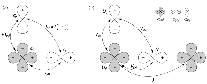
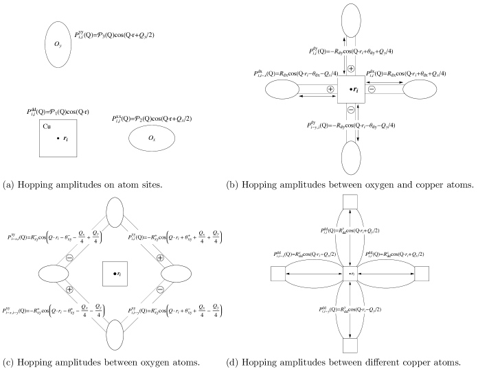
For tppi=0superscriptsubscript𝑡𝑝𝑝𝑖0t_{pp}^{i}=0, this Hamiltonian reduces to the Emery model and corresponds to the tight-binding model of the unit cell shown in Fig. 1(a). The signs of the Cu-O hopping amplitudes are determined by the phases of neighboring lobes of the orbital wavefunctions. In order to obtain a realistic Fermi surface for the cuprates, however, we must impose that the direct hopping amplitude between oxygen orbitals tppdsuperscriptsubscript𝑡𝑝𝑝𝑑t_{pp}^{d} be negative by hand. This is unsatisfactory since we would normally expect that tppdsuperscriptsubscript𝑡𝑝𝑝𝑑t_{pp}^{d} be positive. By integrating out the Cu 4s𝑠s orbital from a 4-band Hamiltonian, Andersen et al. found a negative indirect hopping amplitude tppisuperscriptsubscript𝑡𝑝𝑝𝑖t_{pp}^{i}. Further, the direct hopping amplitude they calculated was comparatively small. Consequently, in what follows, we have set tppi=1.0superscriptsubscript𝑡𝑝𝑝𝑖1.0t_{pp}^{i}=-1.0 and tppd=0superscriptsubscript𝑡𝑝𝑝𝑑0t_{pp}^{d}=0. The remaining values of the hopping amplitudes are given in Table 1. We note that for computational ease we have chosen our gauge, given in Eq. (26) in Appendix A, so that H^tsubscript^𝐻𝑡\hat{H}_{t} is a real symmetric matrix.

Refer to caption
Figure 1: (a) Diagram of the unit cell of the lattice showing the hopping amplitudes corresponding to the tight-binding Hamiltonian in Eq. 3. The on-site energies ϵdsubscriptitalic-ϵ𝑑\epsilon_{d} and ϵpsubscriptitalic-ϵ𝑝\epsilon_{p} and the inter-orbital hopping parameters tpdsubscript𝑡𝑝𝑑t_{pd} and tppsubscript𝑡𝑝𝑝t_{pp} are displayed next to the corresponding orbitals and bonds respectively. Note how the sign of tpdsubscript𝑡𝑝𝑑t_{pd} changes depending on the relative phases of the wavefunction lobes closest to one another. (b) Diagram showing the interactions of the Hamiltonian within the unit cell and between two nearest-neighbor copper atoms. The corresponding expressions are given in Eqs. 7 and 8.

The Green’s functions are given by diagonalizing the kernel (𝐤)𝐤\mathcal{H}({\mathbf{k}}):

𝐒(𝐤)(𝐤)𝐒(𝐤)=𝚲(𝐤)superscript𝐒𝐤𝐤𝐒𝐤𝚲𝐤\displaystyle\mathbf{S}^{\dagger}({\mathbf{k}})\mathcal{H}({\mathbf{k}})\mathbf{S}({\mathbf{k}})=\mathbf{\Lambda}({\mathbf{k}}) (4)

where Λμν(𝐤)=δμνE𝐤μsubscriptΛ𝜇𝜈𝐤subscript𝛿𝜇𝜈subscriptsuperscript𝐸𝜇𝐤\Lambda_{\mu\nu}({\mathbf{k}})=\delta_{\mu\nu}E^{\mu}_{\mathbf{k}} gives the band energies and 𝐒(𝐤)𝐒𝐤\mathbf{S}({\mathbf{k}}) is a 3×3333\times 3 matrix of eigenvectors. In the diagonal basis, the bare Green’s function is

𝒢γ0(𝐤;ωn)=1iωn(E𝐤γμ)subscriptsuperscript𝒢0𝛾𝐤subscript𝜔𝑛1𝑖subscript𝜔𝑛subscriptsuperscript𝐸𝛾𝐤𝜇\displaystyle\mathcal{G}^{0}_{\gamma}({\mathbf{k}};\omega_{n})={-1\over i\omega_{n}-(E^{\gamma}_{\mathbf{k}}-\mu)} (5)

and so the Green’s function in the orbital basis is

Gμν0(𝐤;ωn)subscriptsuperscript𝐺0𝜇𝜈𝐤subscript𝜔𝑛\displaystyle G^{0}_{\mu\nu}({\mathbf{k}};\omega_{n}) =γSμγ(𝐤)Sνγ(𝐤)1iωn(E𝐤γμ).absentsubscript𝛾subscriptsuperscript𝑆𝜇𝛾𝐤subscript𝑆𝜈𝛾𝐤1𝑖subscript𝜔𝑛subscriptsuperscript𝐸𝛾𝐤𝜇\displaystyle=-\sum_{\gamma}S^{*}_{\mu\gamma}({\mathbf{k}})S_{\nu\gamma}({\mathbf{k}}){1\over i\omega_{n}-(E^{\gamma}_{\mathbf{k}}-\mu)}\,. (6)

We consider the effect of two types of interactions. The first is the Coulomb interaction H^Csubscript^𝐻𝐶\hat{H}_{C}, which we further separate into a Hubbard term, H^Chsuperscriptsubscript^𝐻𝐶\hat{H}_{C}^{h}, and an inter-orbital term, H^Cvsuperscriptsubscript^𝐻𝐶𝑣\hat{H}_{C}^{v}:

H^C=subscript^𝐻𝐶absent\displaystyle\hat{H}_{C}= H^Ch+H^Cvsuperscriptsubscript^𝐻𝐶superscriptsubscript^𝐻𝐶𝑣\displaystyle\hat{H}_{C}^{h}+\hat{H}_{C}^{v} (7)
H^Ch=superscriptsubscript^𝐻𝐶absent\displaystyle\hat{H}_{C}^{h}= i[Udcd(𝐫i)cd(𝐫i)cd(𝐫i)cd(𝐫i)+Up(cx(𝐫i)cx(𝐫i)cx(𝐫i)cx(𝐫i)+cy(𝐫i)cy(𝐫i)cy(𝐫i)cy(𝐫i))]subscript𝑖delimited-[]subscript𝑈𝑑superscriptsubscript𝑐𝑑absentsubscript𝐫𝑖subscript𝑐𝑑absentsubscript𝐫𝑖superscriptsubscript𝑐𝑑absentsubscript𝐫𝑖subscript𝑐𝑑absentsubscript𝐫𝑖subscript𝑈𝑝superscriptsubscript𝑐𝑥absentsubscript𝐫𝑖subscript𝑐𝑥absentsubscript𝐫𝑖superscriptsubscript𝑐𝑥absentsubscript𝐫𝑖subscript𝑐𝑥absentsubscript𝐫𝑖superscriptsubscript𝑐𝑦absentsubscript𝐫𝑖subscript𝑐𝑦absentsubscript𝐫𝑖superscriptsubscript𝑐𝑦absentsubscript𝐫𝑖subscript𝑐𝑦absentsubscript𝐫𝑖\displaystyle\sum_{i}\left[U_{d}\,c_{d\uparrow}^{\dagger}({\mathbf{r}}_{i})c_{d\uparrow}({\mathbf{r}}_{i})c_{d\downarrow}^{\dagger}({\mathbf{r}}_{i})c_{d\downarrow}({\mathbf{r}}_{i})+U_{p}\left(c_{x\uparrow}^{\dagger}({\mathbf{r}}_{i})c_{x\uparrow}({\mathbf{r}}_{i})c_{x\downarrow}^{\dagger}({\mathbf{r}}_{i})c_{x\downarrow}({\mathbf{r}}_{i})+c_{y\uparrow}^{\dagger}({\mathbf{r}}_{i})c_{y\uparrow}({\mathbf{r}}_{i})c_{y\downarrow}^{\dagger}({\mathbf{r}}_{i})c_{y\downarrow}({\mathbf{r}}_{i})\right)\right]
H^Cv=superscriptsubscript^𝐻𝐶𝑣absent\displaystyle\hat{H}_{C}^{v}= ijVpdcdα(𝐫i)cdα(𝐫i)[cxβ(𝐫j)cxβ(𝐫j)+cyβ(𝐫j)cyβ(𝐫j)]subscriptexpectation𝑖𝑗subscript𝑉𝑝𝑑superscriptsubscript𝑐𝑑𝛼subscript𝐫𝑖subscript𝑐𝑑𝛼subscript𝐫𝑖delimited-[]superscriptsubscript𝑐𝑥𝛽subscript𝐫𝑗subscript𝑐𝑥𝛽subscript𝐫𝑗superscriptsubscript𝑐𝑦𝛽subscript𝐫𝑗subscript𝑐𝑦𝛽subscript𝐫𝑗\displaystyle\sum_{\braket{ij}}V_{pd}c_{d\alpha}^{\dagger}({\mathbf{r}}_{i})c_{d\alpha}({\mathbf{r}}_{i})\left[c_{x{\beta}}^{\dagger}({\mathbf{r}}_{j})c_{x{\beta}}({\mathbf{r}}_{j})+c_{y{\beta}}^{\dagger}({\mathbf{r}}_{j})c_{y{\beta}}({\mathbf{r}}_{j})\right]
+ijVppcxα(𝐫i)cxα(𝐫i)cyβ(𝐫j)cyβ(𝐫j)subscriptexpectation𝑖𝑗subscript𝑉𝑝𝑝superscriptsubscript𝑐𝑥𝛼subscript𝐫𝑖subscript𝑐𝑥𝛼subscript𝐫𝑖superscriptsubscript𝑐𝑦𝛽subscript𝐫𝑗subscript𝑐𝑦𝛽subscript𝐫𝑗\displaystyle+\sum_{\braket{ij}}V_{pp}c_{x\alpha}^{\dagger}({\mathbf{r}}_{i})c_{x\alpha}({\mathbf{r}}_{i})c_{y{\beta}}^{\dagger}({\mathbf{r}}_{j})c_{y{\beta}}({\mathbf{r}}_{j})

where the sums in the last two lines are over nearest-neighbors. We go beyond the previous work Atkinson et al. (2015); Bulut et al. (2013) by also including a direct exchange term between the Cu atoms

H^J=ijaJ4σαβaσγδacdα(𝐫i)cdβ(𝐫i)cdγ(𝐫j)cdδ(𝐫j),subscript^𝐻𝐽subscriptexpectation𝑖𝑗subscript𝑎𝐽4subscriptsuperscript𝜎𝑎𝛼𝛽subscriptsuperscript𝜎𝑎𝛾𝛿superscriptsubscript𝑐𝑑𝛼subscript𝐫𝑖subscript𝑐𝑑𝛽subscript𝐫𝑖superscriptsubscript𝑐𝑑𝛾subscript𝐫𝑗subscript𝑐𝑑𝛿subscript𝐫𝑗\displaystyle\hat{H}_{J}=\sum_{\braket{ij}}\sum_{a}{J\over 4}\sigma^{a}_{\alpha{\beta}}\sigma^{a}_{\gamma\delta}c_{d\alpha}^{\dagger}({\mathbf{r}}_{i})c_{d{\beta}}({\mathbf{r}}_{i})c_{d\gamma}^{\dagger}({\mathbf{r}}_{j})c_{d\delta}({\mathbf{r}}_{j})\,, (8)

where the sum is over nearest-neighbor interactions between Cu atoms in different unit cells. The interactions between the various orbitals are shown in Fig. 1(b). The full Hamiltonian is given by the sum

H^=H^t+H^C+H^J.^𝐻subscript^𝐻𝑡subscript^𝐻𝐶subscript^𝐻𝐽\displaystyle\hat{H}=\hat{H}_{t}+\hat{H}_{C}+\hat{H}_{J}\,. (9)

We transform the interaction terms to momentum space, and express them using a suitable set of basis functions in Appendix A. For the particle-hole singlet channel which we wish to study, 23 basis functions are required. This can easily be seen by counting the number on-site and inter-orbital interactions present in the Hamiltonian. The Hubbard term has on-site copper, O pxsubscript𝑝𝑥p_{x}, and O pysubscript𝑝𝑦p_{y} orbital interactions and, since they are local, they require one basis function each. Conversely, the inter-orbital interactions have two separate degrees of freedom. For instance, each copper atom per unit cell interacts through the Coulomb term with 4 distinct oxygen orbitals, and so requires 8 basis functions. Similarly, the interactions among the O pxsubscript𝑝𝑥p_{x} and O pysubscript𝑝𝑦p_{y} orbitals and between the copper orbitals in different unit cells introduce another 12 basis functions. These are given in Table 3 in Appendix A.

As mentioned above, we are primarily interested in the density wave instability of this model in the particle-hole channel. In order to do study this, we generalize the order parameter defined in Eq. (1) to the 3-band model by the addition of orbital indices. Accounting for the gauge choice given in Eq. (26), we write

Pijμνsuperscriptsubscript𝑃𝑖𝑗𝜇𝜈\displaystyle P_{ij}^{\mu\nu} =cμα(𝐫i)cνα(𝐫j)=𝔷μν𝐐[d2k4π2P𝐐μν(𝐤)ei𝐤(𝐫i𝐫j)ei𝐤(𝐑μ𝐑ν)]ei𝐐(𝐫i+𝐫j)/2ei𝐐(𝐑μ+𝐑ν)/2absentexpectationsuperscriptsubscript𝑐𝜇𝛼subscript𝐫𝑖subscript𝑐𝜈𝛼subscript𝐫𝑗subscript𝔷𝜇𝜈subscript𝐐delimited-[]superscript𝑑2𝑘4superscript𝜋2subscriptsuperscript𝑃𝜇𝜈𝐐𝐤superscript𝑒𝑖𝐤subscript𝐫𝑖subscript𝐫𝑗superscript𝑒𝑖𝐤subscript𝐑𝜇subscript𝐑𝜈superscript𝑒𝑖𝐐subscript𝐫𝑖subscript𝐫𝑗2superscript𝑒𝑖𝐐subscript𝐑𝜇subscript𝐑𝜈2\displaystyle=\Braket{c_{\mu\alpha}^{\dagger}({\mathbf{r}}_{i})c_{\nu\alpha}({\mathbf{r}}_{j})}={\mathfrak{z}_{\mu\nu}}\sum_{\mathbf{Q}}\left[\int{d^{2}k\over 4\pi^{2}}\,P^{\mu\nu}_{\mathbf{Q}}({\mathbf{k}})e^{i{\mathbf{k}}\cdot({\mathbf{r}}_{i}-{\mathbf{r}}_{j})}e^{i{\mathbf{k}}\cdot(\mathbf{R}_{\mu}-\mathbf{R}_{\nu})}\right]e^{i{\mathbf{Q}}\cdot({\mathbf{r}}_{i}+{\mathbf{r}}_{j})/2}e^{i{\mathbf{Q}}\cdot(\mathbf{R}_{\mu}+\mathbf{R}_{\nu})/2} (10)
𝔷μνsubscript𝔷𝜇𝜈\displaystyle\mathfrak{z}_{\mu\nu} ={1,μν=dd,xx,yy,xy,yxi,μν=dx,dyi,μν=xd,yd.\displaystyle=\left\{\begin{matrix}[l]\phantom{-}1,&\mu\nu=dd,xx,yy,xy,yx\\ -i,&\mu\nu=dx,dy\\ \phantom{-}i,&\mu\nu=xd,yd\end{matrix}\right.\,.

where there is no implied summation of μ𝜇\mu and ν𝜈\nu. In momentum space, the order parameter P𝐐μν(𝐤)subscriptsuperscript𝑃𝜇𝜈𝐐𝐤P^{\mu\nu}_{\mathbf{Q}}({\mathbf{k}}) can also be decomposed into the basis functions given in Table 3:

P𝐐μν(𝐤)subscriptsuperscript𝑃𝜇𝜈𝐐𝐤\displaystyle P^{\mu\nu}_{\mathbf{Q}}({\mathbf{k}}) =𝔷μνl=123𝒫l(𝐐)ϕμνl(𝐤).absentsubscript𝔷𝜇𝜈superscriptsubscript𝑙123subscript𝒫𝑙𝐐subscriptsuperscriptitalic-ϕ𝑙𝜇𝜈𝐤\displaystyle=\mathfrak{z}_{\mu\nu}\sum_{l=1}^{23}\mathcal{P}_{l}({\mathbf{Q}})\phi^{\,l}_{\mu\nu}({\mathbf{k}})\,. (11)

Hermiticity requires that Pijμν=(Pjiνμ)subscriptsuperscript𝑃𝜇𝜈𝑖𝑗superscriptsubscriptsuperscript𝑃𝜈𝜇𝑗𝑖P^{\mu\nu}_{ij}=\left(P^{\nu\mu}_{ji}\right)^{*} and it follows that in momentum space

P𝐐μν(𝐤)=(P𝐐νμ(𝐤)).subscriptsuperscript𝑃𝜇𝜈𝐐𝐤superscriptsubscriptsuperscript𝑃𝜈𝜇𝐐𝐤\displaystyle P^{\mu\nu}_{{\mathbf{Q}}}({\mathbf{k}})=\left(P^{\nu\mu}_{-{\mathbf{Q}}}({\mathbf{k}})\right)^{*}. (12)

Because of the Fourier definition in Eq. (26), time reversal 𝒯𝒯\mathcal{T} acts on the electron annihilation operator cμα(𝐤)subscript𝑐𝜇𝛼𝐤c_{\mu\alpha}({\mathbf{k}}) as

𝒯cμ(𝐤)𝒯1=ημνcμ(𝐤),η=diag(1,1,1).formulae-sequence𝒯subscript𝑐𝜇absent𝐤superscript𝒯1subscript𝜂𝜇𝜈subscript𝑐𝜇absent𝐤𝜂diag111\displaystyle\mathcal{T}c_{\mu\uparrow}({\mathbf{k}})\mathcal{T}^{-1}=\eta_{\mu\nu}c_{\mu\downarrow}(-{\mathbf{k}}),\qquad\qquad\eta=\text{diag}(1,-1,-1). (13)

It follows that the order parameter transforms as

𝒯:P𝐐μν(𝐤)ημγηνδP𝐐γδ(𝐤).:𝒯maps-tosubscriptsuperscript𝑃𝜇𝜈𝐐𝐤subscript𝜂𝜇𝛾subscript𝜂𝜈𝛿subscriptsuperscript𝑃𝛾𝛿𝐐𝐤\displaystyle\mathcal{T}:P^{\mu\nu}_{{\mathbf{Q}}}({\mathbf{k}})\mapsto\eta_{\mu\gamma}\eta_{\nu\delta}P^{\gamma\delta}_{{\mathbf{Q}}}(-{\mathbf{k}})\,. (14)

The action of 𝒯𝒯\mathcal{T} on the functions 𝒫l(𝐐)subscript𝒫𝑙𝐐\mathcal{P}_{l}({\mathbf{Q}}) is summarized in Table 4 of Appendix A.

II.1 Particle-hole interactions

This subsection will compute the particle-hole ladder diagrams associated with density wave instabilities, and find their eigenmodes (the components {𝒫l(𝐐)}subscript𝒫𝑙𝐐\{\mathcal{P}_{l}({\mathbf{Q}})\} defined in Eq. 11) as a function of the total momentum of the particle-hole pair.

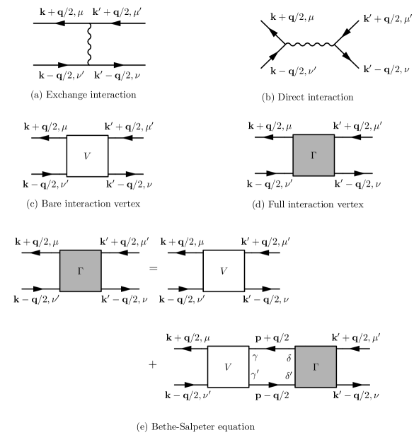
Similar to Ref. Bulut et al. (2013), we accomplish this by reducing the Bethe-Salpeter equation to a matrix equation and numerically solving. We start by defining an effective interaction as a sum between the exchange and direct interactions for the charge channel:

𝐕μμ,νν(𝐤,𝐤,𝐪)=𝐗μμ,νν(𝐤𝐤)2𝐖μμ,νν(𝐪).subscript𝐕𝜇superscript𝜇𝜈superscript𝜈𝐤superscript𝐤𝐪subscript𝐗𝜇superscript𝜇𝜈superscript𝜈𝐤superscript𝐤2subscript𝐖𝜇superscript𝜇𝜈superscript𝜈𝐪\displaystyle\mathbf{V}_{\mu\mu^{\prime},\nu\nu^{\prime}}({\mathbf{k}},{\mathbf{k}}^{\prime},{\mathbf{q}})=\mathbf{X}_{\mu\mu^{\prime},\nu\nu^{\prime}}({\mathbf{k}}-{\mathbf{k}}^{\prime})-2\mathbf{W}_{\mu\mu^{\prime},\nu\nu^{\prime}}({\mathbf{q}})\,. (15)

The exchange 𝐗μμ,ννsubscript𝐗𝜇superscript𝜇𝜈superscript𝜈\mathbf{X}_{\mu\mu^{\prime},\nu\nu^{\prime}} and direct 𝐖μμ,ννsubscript𝐖𝜇superscript𝜇𝜈superscript𝜈\mathbf{W}_{\mu\mu^{\prime},\nu\nu^{\prime}} parts of the interaction are represented in (a) and (b) of Fig. 2 respectively and the bare interaction 𝐕μμ,ννsubscript𝐕𝜇superscript𝜇𝜈superscript𝜈\mathbf{V}_{\mu\mu^{\prime},\nu\nu^{\prime}} corresponds to Fig. 2(c).

Refer to caption
Figure 2: Feynman diagrams used in the T𝑇T-matrix calculation discussed in Section II.1. (a) and (b) give the exchange and direct interactions respectively. Together, they compose the bare vertex shown in (c) as per Eq. 15. (d) shows the full interaction vertex, which is determined by the Bethe-Salpeter equation given diagrammatically in (e). Further details are presented in the main text.

In terms of the 23 basis functions, we write the exchange vertex as

𝐗μμ,νν(𝐤𝐤)=l,m=123ϕμνl(𝐤)Xlmϕμνm(𝐤)subscript𝐗𝜇superscript𝜇𝜈superscript𝜈𝐤superscript𝐤superscriptsubscript𝑙𝑚123superscriptsubscriptitalic-ϕ𝜇superscript𝜈𝑙𝐤subscript𝑋𝑙𝑚superscriptsubscriptitalic-ϕsuperscript𝜇𝜈𝑚superscript𝐤\displaystyle\mathbf{X}_{\mu\mu^{\prime},\nu\nu^{\prime}}({\mathbf{k}}-{\mathbf{k}}^{\prime})=\sum_{l,m=1}^{23}\phi_{\mu\nu^{\prime}}^{\,l}({\mathbf{k}})X_{lm}\phi_{\mu^{\prime}\nu}^{\,m}({\mathbf{k}}^{\prime}) (16)

where Xlm=𝒱lδlmsubscript𝑋𝑙𝑚subscript𝒱𝑙subscript𝛿𝑙𝑚X_{lm}=\mathcal{V}_{l}\delta_{lm} and 𝒱lsubscript𝒱𝑙\mathcal{V}_{l} are interaction parameters whose relation to the values presented in Table 1 are given in Eq. (31). Similarly, the direct vertex is expressed as

𝐖μμ,νν(𝐪)=l,m=123ϕμνlWlm(𝐪)ϕμνmsubscript𝐖𝜇superscript𝜇𝜈superscript𝜈𝐪superscriptsubscript𝑙𝑚123superscriptsubscriptitalic-ϕ𝜇superscript𝜈𝑙subscript𝑊𝑙𝑚𝐪superscriptsubscriptitalic-ϕsuperscript𝜇𝜈𝑚\displaystyle\mathbf{W}_{\mu\mu^{\prime},\nu\nu^{\prime}}({\mathbf{q}})=\sum_{l,m=1}^{23}{\phi_{\mu\nu^{\prime}}^{l}}\,W_{lm}({\mathbf{q}})\phi_{\mu^{\prime}\nu}^{\,m} (17)

where for l,m>3𝑙𝑚3l,m>3, Wlm(𝐪)=0subscript𝑊𝑙𝑚𝐪0W_{lm}({\mathbf{q}})=0 and for l,m=1,2,3formulae-sequence𝑙𝑚123l,m=1,2,3, it is given by

Wlm(𝐪)=(Ud2Vpdcos(qx/2)2Vpdcos(qy/2)2Vpdcos(qx/2)Up4Vppcos(qx/2)cos(qy/2)2Vpdcos(qy/2)4Vppcos(qx/2)cos(qy/2)Up)lmsubscript𝑊𝑙𝑚𝐪subscriptmatrixsubscript𝑈𝑑2subscript𝑉𝑝𝑑subscript𝑞𝑥22subscript𝑉𝑝𝑑subscript𝑞𝑦22subscript𝑉𝑝𝑑subscript𝑞𝑥2subscript𝑈𝑝4subscript𝑉𝑝𝑝subscript𝑞𝑥2subscript𝑞𝑦22subscript𝑉𝑝𝑑subscript𝑞𝑦24subscript𝑉𝑝𝑝subscript𝑞𝑥2subscript𝑞𝑦2subscript𝑈𝑝𝑙𝑚\displaystyle W_{lm}({\mathbf{q}})=\begin{pmatrix}U_{d}&2V_{pd}\cos(q_{x}/2)&2V_{pd}\cos(q_{y}/2)\\ 2V_{pd}\cos(q_{x}/2)&U_{p}&4V_{pp}\cos(q_{x}/2)\cos(q_{y}/2)\\ 2V_{pd}\cos(q_{y}/2)&4V_{pp}\cos(q_{x}/2)\cos(q_{y}/2)&U_{p}\end{pmatrix}_{lm} (18)

Note that for l,m=1,2,3formulae-sequence𝑙𝑚123l,m=1,2,3, the basis functions ϕμνlsubscriptsuperscriptitalic-ϕ𝑙𝜇𝜈\phi^{\,l}_{\mu\nu} are indeed independent of 𝐤𝐤{\mathbf{k}}.

The leading instability of the total vertex 𝚪μμ,νν(𝐤,𝐤,𝐪)subscript𝚪𝜇superscript𝜇𝜈superscript𝜈𝐤superscript𝐤𝐪\mathbf{\Gamma}_{\mu\mu^{\prime},\nu\nu^{\prime}}({\mathbf{k}},{\mathbf{k}}^{\prime},{\mathbf{q}}), shown in the diagram in Fig. 2(d), defines the order parameter and ordering wavevector we are interested in. We approximate it by a generalized RPA (Bethe-Salpeter equation) scheme as

𝚪μμ,νν(𝐤,\displaystyle\mathbf{\Gamma}_{\mu\mu^{\prime},\nu\nu^{\prime}}({\mathbf{k}}, 𝐤,𝐪)=l,m=123ϕlμν(𝐤)Γlm(𝐪)ϕmμν(𝐤)\displaystyle{\mathbf{k}}^{\prime},{\mathbf{q}})=\sum_{l,m=1}^{23}\phi^{\,l}_{\mu\nu^{\prime}}({\mathbf{k}})\Gamma_{lm}({\mathbf{q}})\phi^{\,m}_{\mu^{\prime}\nu}({\mathbf{k}}^{\prime}) (19)
=l,m=123ϕμνl(𝐤)Vlm(𝐪)ϕμνm(𝐤)absentsuperscriptsubscript𝑙𝑚123subscriptsuperscriptitalic-ϕ𝑙𝜇superscript𝜈𝐤subscript𝑉𝑙𝑚𝐪subscriptsuperscriptitalic-ϕ𝑚superscript𝜇𝜈superscript𝐤\displaystyle=\sum_{l,m=1}^{23}\phi^{l}_{\mu\nu^{\prime}}({\mathbf{k}})V_{lm}({\mathbf{q}})\phi^{\,m}_{\mu^{\prime}\nu}({\mathbf{k}}^{\prime})
+l,m=123n,s=123γγδδ𝐩,ωnϕμνl(𝐤)Vln(𝐪)ϕγγn(𝐩)Gδγ0(𝐩𝐪/2;ωn)Gγδ0(𝐩+𝐪/2;ωn)ϕδδs(𝐩)Γsm(𝐪)ϕμνm(𝐤).superscriptsubscript𝑙𝑚123superscriptsubscript𝑛𝑠123subscript𝛾superscript𝛾𝛿superscript𝛿subscript𝐩subscript𝜔𝑛subscriptsuperscriptitalic-ϕ𝑙𝜇superscript𝜈𝐤subscript𝑉𝑙𝑛𝐪superscriptsubscriptitalic-ϕ𝛾superscript𝛾𝑛𝐩subscriptsuperscript𝐺0superscript𝛿superscript𝛾𝐩𝐪2subscript𝜔𝑛subscriptsuperscript𝐺0𝛾𝛿𝐩𝐪2subscript𝜔𝑛subscriptsuperscriptitalic-ϕ𝑠𝛿superscript𝛿𝐩subscriptΓ𝑠𝑚𝐪subscriptsuperscriptitalic-ϕ𝑚superscript𝜇𝜈superscript𝐤\displaystyle+\sum_{l,m=1}^{23}\sum_{n,s=1}^{23}\sum_{\begin{subarray}{c}\gamma\gamma^{\prime}\\ \delta\delta^{\prime}\end{subarray}}\sum_{{\mathbf{p}},\omega_{n}}\phi^{l}_{\mu\nu^{\prime}}({\mathbf{k}})V_{ln}({\mathbf{q}})\phi_{\gamma\gamma^{\prime}}^{n}({\mathbf{p}})G^{0}_{\delta^{\prime}\gamma^{\prime}}({\mathbf{p}}-{\mathbf{q}}/2;\omega_{n})G^{0}_{\gamma\delta}({\mathbf{p}}+{\mathbf{q}}/2;\omega_{n})\phi^{s}_{\delta\delta^{\prime}}({\mathbf{p}})\Gamma_{sm}({\mathbf{q}})\phi^{m}_{\mu^{\prime}\nu}({\mathbf{k}}^{\prime}).

The corresponding diagrammatic expression is shown in Fig. 2(e). To simplify, we define the polarizability to be

Πns(𝐪)subscriptΠ𝑛𝑠𝐪\displaystyle\Pi_{ns}({\mathbf{q}}) =2γγδδ𝐩,ωnϕγγn(𝐩)Gδγ0(𝐩𝐪/2)Gγδ0(𝐩+𝐪/2)ϕδδs(𝐩)absent2subscript𝛾superscript𝛾𝛿superscript𝛿subscript𝐩subscript𝜔𝑛superscriptsubscriptitalic-ϕ𝛾superscript𝛾𝑛𝐩subscriptsuperscript𝐺0superscript𝛿superscript𝛾𝐩𝐪2subscriptsuperscript𝐺0𝛾𝛿𝐩𝐪2subscriptsuperscriptitalic-ϕ𝑠𝛿superscript𝛿𝐩\displaystyle=2\sum_{\begin{subarray}{c}\gamma\gamma^{\prime}\\ \delta\delta^{\prime}\end{subarray}}\sum_{{\mathbf{p}},\omega_{n}}\phi_{\gamma\gamma^{\prime}}^{n}({\mathbf{p}})G^{0}_{\delta^{\prime}\gamma^{\prime}}({\mathbf{p}}-{\mathbf{q}}/2)G^{0}_{\gamma\delta}({\mathbf{p}}+{\mathbf{q}}/2)\phi^{s}_{\delta\delta^{\prime}}({\mathbf{p}}) (20)
=2𝐩γγδδααϕγγn(𝐩)ϕδδs(𝐩)αα,𝐩𝐪δγγδf(Eα(𝐩𝐪/2))f(Eα(𝐩+𝐪/2))Eα(𝐩𝐪/2)Eα(𝐩+𝐪/2)absent2subscript𝐩subscript𝛾superscript𝛾𝛿superscript𝛿subscript𝛼superscript𝛼subscriptsuperscriptitalic-ϕ𝑛𝛾superscript𝛾𝐩subscriptsuperscriptitalic-ϕ𝑠𝛿superscript𝛿𝐩subscriptsuperscriptsuperscript𝛿superscript𝛾𝛾𝛿superscript𝛼𝛼𝐩𝐪𝑓subscript𝐸superscript𝛼𝐩𝐪2𝑓subscript𝐸𝛼𝐩𝐪2subscript𝐸superscript𝛼𝐩𝐪2subscript𝐸𝛼𝐩𝐪2\displaystyle=-2\sum_{{\mathbf{p}}}\sum_{\begin{subarray}{c}\gamma\gamma^{\prime}\\ \delta\delta^{\prime}\end{subarray}}\sum_{\alpha\alpha^{\prime}}\phi^{\,n}_{\gamma\gamma^{\prime}}({\mathbf{p}})\phi^{\,s}_{\delta\delta^{\prime}}({\mathbf{p}})\mathcal{M}^{\delta^{\prime}\gamma^{\prime}\gamma\delta}_{\alpha^{\prime}\alpha,{\mathbf{p}}{\mathbf{q}}}{f(E_{\alpha^{\prime}}({\mathbf{p}}-{\mathbf{q}}/2))-f(E_{\alpha}({\mathbf{p}}+{\mathbf{q}}/2))\over E_{\alpha^{\prime}}({\mathbf{p}}-{\mathbf{q}}/2)-E_{\alpha}({\mathbf{p}}+{\mathbf{q}}/2)}

where f𝑓f is the Fermi function and

αα,𝐩𝐪δγγδ=Sδα(𝐩𝐪/2)Sγα(𝐩𝐪/2)Sγα(𝐩+𝐪/2)Sδα(𝐩+𝐪/2).subscriptsuperscriptsuperscript𝛿superscript𝛾𝛾𝛿superscript𝛼𝛼𝐩𝐪subscriptsuperscript𝑆superscript𝛿superscript𝛼𝐩𝐪2subscript𝑆superscript𝛾superscript𝛼𝐩𝐪2subscriptsuperscript𝑆𝛾𝛼𝐩𝐪2subscript𝑆𝛿𝛼𝐩𝐪2\displaystyle\mathcal{M}^{\delta^{\prime}\gamma^{\prime}\gamma\delta}_{\alpha^{\prime}\alpha,{\mathbf{p}}{\mathbf{q}}}=S^{*}_{\delta^{\prime}\alpha^{\prime}}({\mathbf{p}}-{\mathbf{q}}/2)S_{\gamma^{\prime}\alpha^{\prime}}({\mathbf{p}}-{\mathbf{q}}/2)S^{*}_{\gamma\alpha}({\mathbf{p}}+{\mathbf{q}}/2)S_{\delta\alpha}({\mathbf{p}}+{\mathbf{q}}/2)\,. (21)

As indicated, it follows that Eq. (19) can be reduced to a matrix equation:

Γlm(𝐪)subscriptΓ𝑙𝑚𝐪\displaystyle\Gamma_{lm}({\mathbf{q}}) =Vlm(𝐪)+12n,s=123Vln(𝐪)Πns(𝐪)Γsm(𝐪)absentsubscript𝑉𝑙𝑚𝐪12superscriptsubscript𝑛𝑠123subscript𝑉𝑙𝑛𝐪subscriptΠ𝑛𝑠𝐪subscriptΓ𝑠𝑚𝐪\displaystyle=V_{lm}({\mathbf{q}})+{1\over 2}\sum_{n,s=1}^{23}V_{ln}({\mathbf{q}})\Pi_{ns}({\mathbf{q}})\Gamma_{sm}({\mathbf{q}}) (22)
=𝒱lδlm2Wlm(𝐪)+12s=123𝒱lΠls(𝐪)Γsm(𝐪)n,s=123Wln(𝐪)Πns(𝐪)Γsm(𝐪).absentsubscript𝒱𝑙subscript𝛿𝑙𝑚2subscript𝑊𝑙𝑚𝐪12superscriptsubscript𝑠123subscript𝒱𝑙subscriptΠ𝑙𝑠𝐪subscriptΓ𝑠𝑚𝐪superscriptsubscript𝑛𝑠123subscript𝑊𝑙𝑛𝐪subscriptΠ𝑛𝑠𝐪subscriptΓ𝑠𝑚𝐪\displaystyle=\mathcal{V}_{l}\delta_{lm}-2W_{lm}({\mathbf{q}})+{1\over 2}\sum_{s=1}^{23}\mathcal{V}_{l}\Pi_{ls}({\mathbf{q}})\Gamma_{sm}({\mathbf{q}})-\sum_{n,s=1}^{23}W_{ln}({\mathbf{q}})\Pi_{ns}({\mathbf{q}})\Gamma_{sm}({\mathbf{q}})\,.

The instabilities of the total vertex are determined by finding the minimum eigenvalues λ𝐪subscript𝜆𝐪\lambda_{\mathbf{q}} of the matrix

Alm(𝐪)=δlm12n=123Vln(𝐪)Πnm(𝐪).subscript𝐴𝑙𝑚𝐪subscript𝛿𝑙𝑚12superscriptsubscript𝑛123subscript𝑉𝑙𝑛𝐪subscriptΠ𝑛𝑚𝐪\displaystyle A_{lm}({\mathbf{q}})=\delta_{lm}-{1\over 2}\sum_{n=1}^{23}V_{ln}({\mathbf{q}})\Pi_{nm}({\mathbf{q}})\,. (23)

for all 𝐪𝐪{\mathbf{q}}. The ordering wavevector corresponds to the 𝐐msubscript𝐐𝑚{\mathbf{Q}}_{m} for which λ𝐐msubscript𝜆subscript𝐐𝑚\lambda_{{\mathbf{Q}}_{m}} is the global minimum over the entire Brillouin zone and the order parameter is defined by the associated eigenvector {𝒫l(𝐐m)}subscript𝒫𝑙subscript𝐐𝑚\{\mathcal{P}_{l}({\mathbf{Q}}_{m})\} through Eq. 11.

II.2 Results

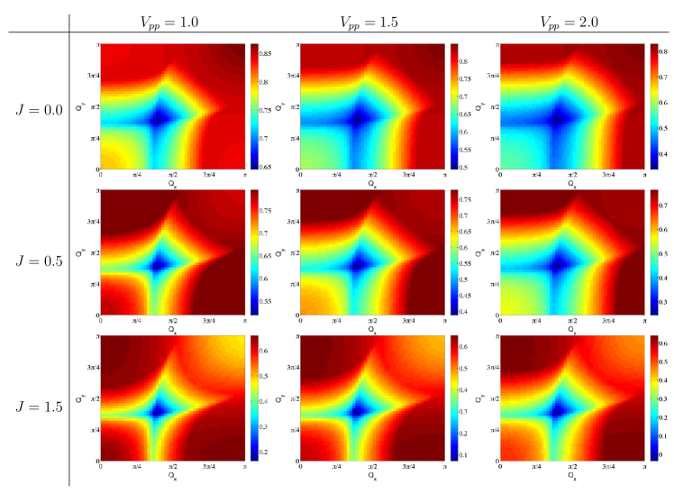
The lowest eigenvalues of the matrix in Eq. (23) as a function of the total momentum 𝐐𝐐{\mathbf{Q}} are plotted in Fig. 3 for a range of parameters. The diagonal wavevector 𝐐=Qm(1,1)𝐐subscript𝑄𝑚11{\mathbf{Q}}=Q_{m}(1,1) for Qm=1.19381subscript𝑄𝑚1.19381Q_{m}=1.19381 point is very consistently the global minimum for a wide range of interaction parameters. Increasing either J𝐽J or Vppsubscript𝑉𝑝𝑝V_{pp} both have the effect of decreasing the minimum eigenvalue. However, larger J𝐽J tends to localize the minimum at Qm(1,1)subscript𝑄𝑚11Q_{m}(1,1) whereas larger Vppsubscript𝑉𝑝𝑝V_{pp} has the opposite effect. A ridge of local minima extending down to the axial wavevector 𝐐=Qm(1,0),Qm(0,1)𝐐subscript𝑄𝑚10subscript𝑄𝑚01{\mathbf{Q}}=Q_{m}(1,0),\,Q_{m}(0,1) is also consistently present. Motivated by experiment, we discuss the order parameters associated with these wavevectors as well.
Refer to caption
Figure 3: (Color online) Plot of the minimum eigenvalue of the matrix Alm(𝐐)subscript𝐴𝑙𝑚𝐐A_{lm}({\mathbf{Q}}) in Eq. (23) for 𝐐𝐐{\mathbf{Q}} in the first quadrant at different values of J𝐽J and Vppsubscript𝑉𝑝𝑝V_{pp}. The temperature is T=0.015𝑇0.015T=0.015 and the filling p=5n=0.1643𝑝5𝑛0.1643p=5-n=0.1643. All other parameters are as given in Table 1. The diagonal point 𝐐=Qm(1,1)𝐐subscript𝑄𝑚11{\mathbf{Q}}=Q_{m}(1,1) for Qm=1.19381subscript𝑄𝑚1.19381Q_{m}=1.19381 is very consistently the point of greatest instability.

Some of the eigenvectors corresponding to both the diagonal and axial momenta are given in Table 2. The d𝑑d-wave character of the order parameter is somewhat harder to read off than in a one band model. As expected, for 𝐐=Qm(1,1)𝐐subscript𝑄𝑚11{\mathbf{Q}}=Q_{m}(1,1), both the on-site Copper amplitude (l=1𝑙1l=1) and the extended s𝑠s-wave symmetry (l=21𝑙21l=21) vanish. For all three vectors presented, the weight is split primarily between the l=2,3𝑙23l=2,3 (on-site O pxsubscript𝑝𝑥p_{x} and O pysubscript𝑝𝑦p_{y} amplitudes) and the l=20𝑙20l=20 (Cu-Cu d𝑑d-form factor) basis vectors. Further, the l=2𝑙2l=2 and l=3𝑙3l=3 components are of the same order of magnitude and have opposite sign, indicating that these vectors are in fact primarily d𝑑d-wave.

At 𝐐=Qm(1,0)𝐐subscript𝑄𝑚10{\mathbf{Q}}=Q_{m}(1,0), the order parameter is similarly primarily d𝑑d-wave in character, though the s𝑠s and ssuperscript𝑠s^{\prime} components no longer vanish. As Vppsubscript𝑉𝑝𝑝V_{pp} is increased, the d𝑑d-wave character also increases.

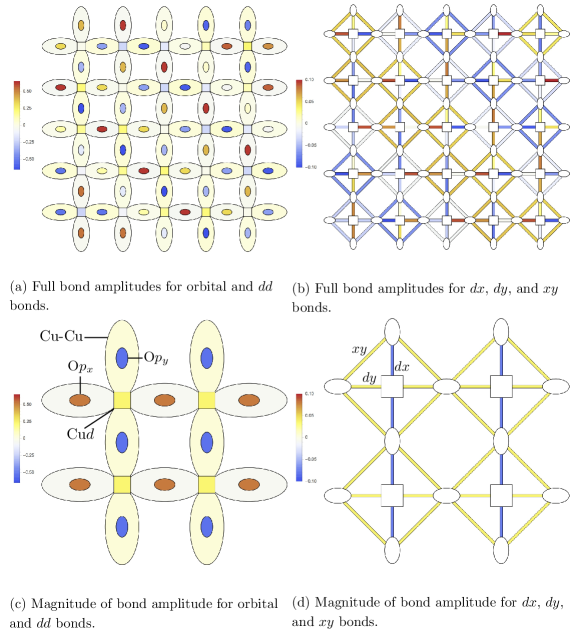
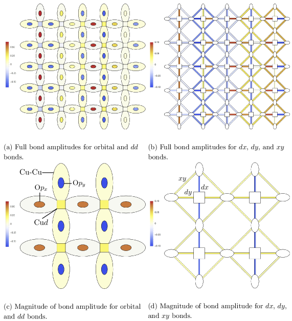
Figs. 4 and 5 are visualizations of the amplitudes given by the order parameter P𝐐μν(𝐤)subscriptsuperscript𝑃𝜇𝜈𝐐𝐤P^{\mu\nu}_{\mathbf{Q}}({\mathbf{k}}) at 𝐐=Qm(1,1)𝐐subscript𝑄𝑚11{\mathbf{Q}}=Q_{m}(1,1) and 𝐐=Qm(1,0)𝐐subscript𝑄𝑚10{\mathbf{Q}}=Q_{m}(1,0) respectively. They are generated by taking the functions listed in Table 5 of Appendix A and plotting a corresponding color. Both with and without the spatial modulation cos𝐐𝐫similar-toabsent𝐐𝐫\sim\cos{\mathbf{Q}}\cdot{\mathbf{r}} envelope are shown for clarity. The primary difference between the two figures is the direction of the amplitude modulation shown in (a) and (b) of either figure. Further, technically, the difference in the colors representing the amplitudes of the O pxsubscript𝑝𝑥p_{x} and O pysubscript𝑝𝑦p_{y} orbitals for the eigenvector at axial momentum in Fig. 5(c) is not as strong as for the diagonal momentum in Fig. 4(c). This follows since, as mentioned, the s𝑠s and ssuperscript𝑠s^{\prime} components of the order parameter in the axial case are nonzero. However, since these components are small, there is little indication of any s𝑠s character.

l𝑙l ϕμνl(𝐤)subscriptsuperscriptitalic-ϕ𝑙𝜇𝜈𝐤\phi^{l}_{\mu\nu}({\mathbf{k}}) Qm(1,1)subscript𝑄𝑚11Q_{m}(1,1) Qm(1,0)subscript𝑄𝑚10Q_{m}(1,0)
Vpp=1.0subscript𝑉𝑝𝑝1.0V_{pp}=1.0 Vpp=1.5subscript𝑉𝑝𝑝1.5V_{pp}=1.5 Vpp=2.0subscript𝑉𝑝𝑝2.0V_{pp}=2.0 Vpp=1.0subscript𝑉𝑝𝑝1.0V_{pp}=1.0 Vpp=1.5subscript𝑉𝑝𝑝1.5V_{pp}=1.5 Vpp=2.0subscript𝑉𝑝𝑝2.0V_{pp}=2.0
111 δμdδνdsubscript𝛿𝜇𝑑subscript𝛿𝜈𝑑\delta_{\mu d}\,\delta_{\nu d} 0.00.0\phantom{-}0.0 0.00.0\phantom{-}0.0 0.00.0\phantom{-}0.0 0.34170.3417-0.3417 0.23480.2348-0.2348 0.18480.1848-0.1848
222 δμxδνxsubscript𝛿𝜇𝑥subscript𝛿𝜈𝑥\delta_{\mu x}\,\delta_{\nu x} 0.46360.4636-0.4636 0.61850.6185-0.6185 0.65920.6592-0.6592 0.52520.5252-0.5252 0.63610.6361-0.6361 0.66590.6659-0.6659
333 δμyδνysubscript𝛿𝜇𝑦subscript𝛿𝜈𝑦\delta_{\mu y}\,\delta_{\nu y} 0.46360.4636\phantom{-}0.4636 0.61850.6185\phantom{-}0.6185 0.65920.6592\phantom{-}0.6592 0.54260.5426\phantom{-}0.5426 0.65000.6500\phantom{-}0.6500 0.67560.6756\phantom{-}0.6756
444 δμdδνx2cos(kx2)subscript𝛿𝜇𝑑subscript𝛿𝜈𝑥2subscript𝑘𝑥2\delta_{\mu d}\,\delta_{\nu x}\sqrt{2}\cos\left({k_{x}\over 2}\right) 0.20170.2017-0.2017 0.11840.1184-0.1184 0.07890.0789-0.0789 0.20650.2065-0.2065 0.11350.1135-0.1135 0.07510.0751-0.0751
555 δμxδνd2cos(kx2)subscript𝛿𝜇𝑥subscript𝛿𝜈𝑑2subscript𝑘𝑥2\delta_{\mu x}\,\delta_{\nu d}\sqrt{2}\cos\left({k_{x}\over 2}\right) 0.20170.2017\phantom{-}0.2017 0.11840.1184\phantom{-}0.1184 0.07890.0789\phantom{-}0.0789 0.20650.2065\phantom{-}0.2065 0.11350.1135\phantom{-}0.1135 0.07510.0751\phantom{-}0.0751
666 δμdδνx2sin(kx2)subscript𝛿𝜇𝑑subscript𝛿𝜈𝑥2subscript𝑘𝑥2\delta_{\mu d}\,\delta_{\nu x}\sqrt{2}\sin\left({k_{x}\over 2}\right) 0.23010.2301-0.2301 0.13740.1374-0.1374 0.09270.0927-0.0927 0.16180.1618-0.1618 0.09170.0917-0.0917 0.06120.0612-0.0612
777 δμxδνd2sin(kx2)subscript𝛿𝜇𝑥subscript𝛿𝜈𝑑2subscript𝑘𝑥2\delta_{\mu x}\,\delta_{\nu d}\sqrt{2}\sin\left({k_{x}\over 2}\right) 0.23010.2301-0.2301 0.13740.1374-0.1374 0.09270.0927-0.0927 0.16180.1618-0.1618 0.09170.0917-0.0917 0.06120.0612-0.0612
888 δμdδνy2cos(ky2)subscript𝛿𝜇𝑑subscript𝛿𝜈𝑦2subscript𝑘𝑦2\delta_{\mu d}\,\delta_{\nu y}\sqrt{2}\cos\left({k_{y}\over 2}\right) 0.20170.2017-0.2017 0.11840.1184-0.1184 0.07890.0789-0.0789 0.00.0\phantom{-}0.0 0.00.0\phantom{-}0.0 0.00.0\phantom{-}0.0
999 δμyδνd2cos(ky2)subscript𝛿𝜇𝑦subscript𝛿𝜈𝑑2subscript𝑘𝑦2\delta_{\mu y}\,\delta_{\nu d}\sqrt{2}\cos\left({k_{y}\over 2}\right) 0.20170.2017\phantom{-}0.2017 0.11840.1184\phantom{-}0.1184 0.07890.0789\phantom{-}0.0789 0.00.0\phantom{-}0.0 0.00.0\phantom{-}0.0 0.00.0\phantom{-}0.0
101010 δμdδνy2sin(ky2)subscript𝛿𝜇𝑑subscript𝛿𝜈𝑦2subscript𝑘𝑦2\delta_{\mu d}\,\delta_{\nu y}\sqrt{2}\sin\left({k_{y}\over 2}\right) 0.23010.2301-0.2301 0.13740.1374-0.1374 0.09270.0927-0.0927 0.19850.1985-0.1985 0.11540.1154-0.1154 0.07890.0789-0.0789
111111 δμyδνd2sin(ky2)subscript𝛿𝜇𝑦subscript𝛿𝜈𝑑2subscript𝑘𝑦2\delta_{\mu y}\,\delta_{\nu d}\sqrt{2}\sin\left({k_{y}\over 2}\right) 0.23010.2301-0.2301 0.13740.1374-0.1374 0.09270.0927-0.0927 0.19850.1985-0.1985 0.11540.1154-0.1154 0.07890.0789-0.0789
121212 δμxδνy 2cos(kx2)cos(ky2)subscript𝛿𝜇𝑥subscript𝛿𝜈𝑦2subscript𝑘𝑥2subscript𝑘𝑦2\delta_{\mu x}\,\delta_{\nu y}\,2\cos\left({k_{x}\over 2}\right)\cos\left({k_{y}\over 2}\right) 0.00.0\phantom{-}0.0 0.00.0\phantom{-}0.0 0.00.0\phantom{-}0.0 0.00.0\phantom{-}0.0 0.00.0\phantom{-}0.0 0.00.0\phantom{-}0.0
131313 δμyδνx 2cos(kx2)cos(ky2)subscript𝛿𝜇𝑦subscript𝛿𝜈𝑥2subscript𝑘𝑥2subscript𝑘𝑦2\delta_{\mu y}\,\delta_{\nu x}\,2\cos\left({k_{x}\over 2}\right)\cos\left({k_{y}\over 2}\right) 0.00.0\phantom{-}0.0 0.00.0\phantom{-}0.0 0.00.0\phantom{-}0.0 0.00.0\phantom{-}0.0 0.00.0\phantom{-}0.0 0.00.0\phantom{-}0.0
141414 δμxδνy 2cos(kx2)sin(ky2)subscript𝛿𝜇𝑥subscript𝛿𝜈𝑦2subscript𝑘𝑥2subscript𝑘𝑦2\delta_{\mu x}\,\delta_{\nu y}\,2\cos\left({k_{x}\over 2}\right)\sin\left({k_{y}\over 2}\right) 0.14610.1461-0.1461 0.13340.1334-0.1334 0.12130.1213-0.1213 0.15950.1595-0.1595 0.13770.1377-0.1377 0.12420.1242-0.1242
151515 δμyδνx 2cos(kx2)sin(ky2)subscript𝛿𝜇𝑦subscript𝛿𝜈𝑥2subscript𝑘𝑥2subscript𝑘𝑦2\delta_{\mu y}\,\delta_{\nu x}\,2\cos\left({k_{x}\over 2}\right)\sin\left({k_{y}\over 2}\right) 0.14610.1461\phantom{-}0.1461 0.13340.1334\phantom{-}0.1334 0.12130.1213\phantom{-}0.1213 0.15950.1595\phantom{-}0.1595 0.13770.1377\phantom{-}0.1377 0.12420.1242\phantom{-}0.1242
161616 δμxδνy 2sin(kx2)cos(ky2)subscript𝛿𝜇𝑥subscript𝛿𝜈𝑦2subscript𝑘𝑥2subscript𝑘𝑦2\delta_{\mu x}\,\delta_{\nu y}\,2\sin\left({k_{x}\over 2}\right)\cos\left({k_{y}\over 2}\right) 0.14610.1461-0.1461 0.13340.1334-0.1334 0.12130.1213-0.1213 0.00.0\phantom{-}0.0 0.00.0\phantom{-}0.0 0.00.0\phantom{-}0.0
171717 δμyδνx 2sin(kx2)cos(ky2)subscript𝛿𝜇𝑦subscript𝛿𝜈𝑥2subscript𝑘𝑥2subscript𝑘𝑦2\delta_{\mu y}\,\delta_{\nu x}\,2\sin\left({k_{x}\over 2}\right)\cos\left({k_{y}\over 2}\right) 0.14610.1461\phantom{-}0.1461 0.13340.1334\phantom{-}0.1334 0.12130.1213\phantom{-}0.1213 0.00.0\phantom{-}0.0 0.00.0\phantom{-}0.0 0.00.0\phantom{-}0.0
181818 δμxδνy 2sin(kx2)sin(ky2)subscript𝛿𝜇𝑥subscript𝛿𝜈𝑦2subscript𝑘𝑥2subscript𝑘𝑦2\delta_{\mu x}\,\delta_{\nu y}\,2\sin\left({k_{x}\over 2}\right)\sin\left({k_{y}\over 2}\right) 0.00.0\phantom{-}0.0 0.00.0\phantom{-}0.0 0.00.0\phantom{-}0.0 0.00050.0005-0.0005 0.00040.0004-0.0004 0.00010.0001-0.0001
191919 δμyδνx 2sin(kx2)sin(ky2)subscript𝛿𝜇𝑦subscript𝛿𝜈𝑥2subscript𝑘𝑥2subscript𝑘𝑦2\delta_{\mu y}\,\delta_{\nu x}\,2\sin\left({k_{x}\over 2}\right)\sin\left({k_{y}\over 2}\right) 0.00.0\phantom{-}0.0 0.00.0\phantom{-}0.0 0.00.0\phantom{-}0.0 0.00050.0005-0.0005 0.00040.0004-0.0004 0.00010.0001-0.0001
202020 δμdδνd(coskxcosky)subscript𝛿𝜇𝑑subscript𝛿𝜈𝑑subscript𝑘𝑥subscript𝑘𝑦\delta_{\mu d}\,\delta_{\nu d}\left(\cos{k_{x}}-\cos k_{y}\right) 0.33200.3320\phantom{-}0.3320 0.17930.1793\phantom{-}0.1793 0.11300.1130\phantom{-}0.1130 0.21290.2129\phantom{-}0.2129 0.10250.1025\phantom{-}0.1025 0.06240.0624\phantom{-}0.0624
212121 δμdδνd(coskx+cosky)subscript𝛿𝜇𝑑subscript𝛿𝜈𝑑subscript𝑘𝑥subscript𝑘𝑦\delta_{\mu d}\,\delta_{\nu d}\left(\cos{k_{x}}+\cos k_{y}\right) 0.00.0\phantom{-}0.0 0.00.0\phantom{-}0.0 0.00.0\phantom{-}0.0 0.02090.0209\phantom{-}0.0209 0.01120.0112\phantom{-}0.0112 0.00720.0072\phantom{-}0.0072
222222 δμdδνd(sinkxsinky)subscript𝛿𝜇𝑑subscript𝛿𝜈𝑑subscript𝑘𝑥subscript𝑘𝑦\delta_{\mu d}\,\delta_{\nu d}\left(\sin{k_{x}}-\sin k_{y}\right) 0.00.0\phantom{-}0.0 0.00.0\phantom{-}0.0 0.00.0\phantom{-}0.0 0.00.0\phantom{-}0.0 0.00.0\phantom{-}0.0 0.00.0\phantom{-}0.0
232323 δμdδνd(sinkx+sinky)subscript𝛿𝜇𝑑subscript𝛿𝜈𝑑subscript𝑘𝑥subscript𝑘𝑦\delta_{\mu d}\,\delta_{\nu d}\left(\sin{k_{x}}+\sin k_{y}\right) 0.00.0\phantom{-}0.0 0.00.0\phantom{-}0.0 0.00.0\phantom{-}0.0 0.00.0\phantom{-}0.0 0.00.0\phantom{-}0.0 0.00.0\phantom{-}0.0
Table 2: Eigenvectors corresponding to 𝐐=Qm(1,1)𝐐subscript𝑄𝑚11{\mathbf{Q}}=Q_{m}(1,1) and 𝐐=Qm(1,0)𝐐subscript𝑄𝑚10{\mathbf{Q}}=Q_{m}(1,0) for J=0.5𝐽0.5J=0.5, Vpd=1.0subscript𝑉𝑝𝑑1.0V_{pd}=1.0 and Vpp=1.0, 1.5subscript𝑉𝑝𝑝1.01.5V_{pp}=1.0,\,1.5 and 2.02.02.0. The temperature is T=0.015𝑇0.015T=0.015 and the filling p=0.1643𝑝0.1643p=0.1643. All others parameters are as given in Table 1.
Refer to caption
Figure 4: (Color online) Real space representation of hopping amplitudes for diagonal 𝐐=Qm(1,1)𝐐subscript𝑄𝑚11{\mathbf{Q}}=Q_{m}(1,1) evaluated with J=0.5𝐽0.5J=0.5, Vpp=1.25subscript𝑉𝑝𝑝1.25V_{pp}=1.25, and Vpdsubscript𝑉𝑝𝑑V_{pd} at T=0.015𝑇0.015T=0.015 and p=0.1643𝑝0.1643p=0.1643. For clarity the lattice has been divided into two separate pictures. (a) and (c) display the on-site Copper, the on-site oxygen and the copper-copper hopping amplitudes whereas (b) and (d) give the dx𝑑𝑥dx, dy𝑑𝑦dy and xy𝑥𝑦xy bond amplitudes. (a) and (b) plot the full functions given in Table 5 while (c) and (d) simply display the 𝐫=0𝐫0{\mathbf{r}}=0 part. (c) and (d) also indicate which orbitals and bonds the symbols represent. The modulations of the order parameter in the diagonal direction can be seen in (a) and (b) by tracking the colors of the O pxsubscript𝑝𝑥p_{x}, O pysubscript𝑝𝑦p_{y} orbitals and the xy𝑥𝑦xy bonds respectively over several unit cells. The (c) and (d) pictures make the d𝑑d-form factor evident.
Refer to caption
Figure 5: (Color online) Just as in Fig. 4. Real space representation of hopping amplitudes for axial 𝐐=Qm(1,0)𝐐subscript𝑄𝑚10{\mathbf{Q}}=Q_{m}(1,0) evaluated with J=0.5𝐽0.5J=0.5, Vpp=1.25subscript𝑉𝑝𝑝1.25V_{pp}=1.25, and Vpdsubscript𝑉𝑝𝑑V_{pd} at T=0.015𝑇0.015T=0.015 and p=0.1643𝑝0.1643p=0.1643.

The general structure of the pictures in Figs. 4 and 5 are similar to those obtained in Ref. Sachdev and La Placa, 2013 for the one-band model. In the one-band case, the only quantities available were the on-site densities on the Cu sites, and the bond order parameters involving nearest-neighbor pairs of Cu sites. We find very similar modulations in the same quantities here. However, we now also have additional information using the O sites: the on-site densities on the O sites, the bond orders between the nearest-neighbor Cu and O sites, and the diagonal bond orders between pairs of O sites. All of these quantities are also shown in the figures, and their spatial pattern mirrors those of Cu site and bond orders. In particular the modulation on an O site reflects that on the Cu-Cu bond it resides on.

III Small Fermi surfaces with antiferromagnetic order

We next consider the three band model in the presence of a staggered magnetic field pointing in the 𝐱^^𝐱\mathbf{\hat{x}}-direction:

H^tsuperscriptsubscript^𝐻𝑡\displaystyle\hat{{H}}_{t}^{\prime} =H^t+H^AFabsentsubscript^𝐻𝑡subscript^𝐻𝐴𝐹\displaystyle=\hat{H}_{t}+\hat{H}_{AF} (24)

We perform a self-consistent Hartree-Fock analysis in order to determine the static antiferromagnetic (AF) order parameter Mdsubscript𝑀𝑑M_{d} on the copper atom sites. Further, the Coulomb interactions between the copper and oxygen orbitals may induce an antiferromagnetic bond order so that additional AF order parameters, Mpdsubscript𝑀𝑝𝑑M_{pd} and Mppsubscript𝑀𝑝𝑝M_{pp}, are required. It follows that the general extension to the hopping Hamiltonian in Eq. (3) is

H^AF=iei𝐊𝐫iσαβx[\displaystyle\hat{H}_{AF}=-\sum_{i}e^{i{\mathbf{K}}\cdot{\mathbf{r}}_{i}}\sigma^{x}_{\alpha{\beta}}\bigg{[} Mdcdα(𝐫i)cdβ(𝐫i)subscript𝑀𝑑subscriptsuperscript𝑐𝑑𝛼subscript𝐫𝑖subscript𝑐𝑑𝛽subscript𝐫𝑖\displaystyle M_{d}c^{\dagger}_{d\alpha}({\mathbf{r}}_{i})c_{d{\beta}}({\mathbf{r}}_{i}) (25)
+Mpd(cdα(𝐫)cxβ(𝐫)+cdα(𝐫)cxβ(𝐫𝐱^)+cdα(𝐫)cyβ(𝐫)cdα(𝐫)cyβ(𝐫𝐲^)+h.c.)\displaystyle+M_{pd}\big{(}-c_{d\alpha}^{\dagger}({\mathbf{r}})c_{x{\beta}}({\mathbf{r}})+c_{d\alpha}^{\dagger}({\mathbf{r}})c_{x{\beta}}({\mathbf{r}}-\hat{\mathbf{x}})+c_{d\alpha}^{\dagger}({\mathbf{r}})c_{y{\beta}}({\mathbf{r}})-c_{d\alpha}^{\dagger}({\mathbf{r}})c_{y{\beta}}({\mathbf{r}}-\hat{\mathbf{y}})+h.c.\big{)}\phantom{\bigg{]}}
+Mpp(cxα(𝐫)cyβ(𝐫)cxα(𝐫)cyβ(𝐫𝐲^)\displaystyle+M_{pp}\big{(}\,c_{x\alpha}^{\dagger}({\mathbf{r}})c_{y{\beta}}({\mathbf{r}})-c_{x\alpha}^{\dagger}({\mathbf{r}})c_{y{\beta}}({\mathbf{r}}-\hat{\mathbf{y}})
cxα(𝐫𝐱^)cyβ(𝐫)+cxα(𝐫𝐱^)cyβ(𝐫𝐲^)+h.c.)]\displaystyle\phantom{+M_{pp}\big{(}}-c_{x\alpha}^{\dagger}({\mathbf{r}}-\hat{\mathbf{x}})c_{y{\beta}}({\mathbf{r}})+c_{x\alpha}^{\dagger}({\mathbf{r}}-\hat{\mathbf{x}})c_{y{\beta}}({\mathbf{r}}-\hat{\mathbf{y}})+h.c.\big{)}\bigg{]}

where 𝐊=(π,π)𝐊𝜋𝜋{\mathbf{K}}=(\pi,\pi). The sign of the inter-orbital correlations is the same as in the original hopping Hamiltonian (see Figs. 1 and 9). We transform this Hamiltonian to momentum space basis functions in Appendix B, and describe how the magnetic order parameters Mdsubscript𝑀𝑑M_{d}, Mpdsubscript𝑀𝑝𝑑M_{pd}, and Mppsubscript𝑀𝑝𝑝M_{pp} are computed in the Hartree-Fock theory. We find that Mpdsubscript𝑀𝑝𝑑M_{pd} and Mppsubscript𝑀𝑝𝑝M_{pp} have near-vanishing magnitude and they will not be discussed further.

The particle-hole T𝑇T-matrix calculation in the presence of AF order is similar to the one presented in Section II.1, though considerably more complicated due to spin-flip processes. These calculations are presented in Appendix C. While we are still primarily interested in the particle-hole spin singlet channel, the presence of AF order breaks the SU(2) symmetry of the original Hamiltonian causing the charge channel at wavevector 𝐐𝐐{\mathbf{Q}} to mix with the spin channel at wavevector 𝐐+(π,π)𝐐𝜋𝜋{\mathbf{Q}}+(\pi,\pi). However, while the total spin is no longer conserved, the Sxsubscript𝑆𝑥S_{x} component still is and mixing only occurs between the particle-hole pair with total spin S=0𝑆0S=0 and the particle-hole pair with total spin S=1𝑆1S=1 and spin component Sx=0subscript𝑆𝑥0S_{x}=0. Having to track the total spin doubles the number of required basis functions so that the order parameter is a 46-component vector {𝒫l(𝐐)}subscript𝒫𝑙𝐐\{\mathcal{P}_{l}({\mathbf{Q}})\}. This analysis, as well as the basis functions used for the actual calculations, are given in Appendix D. An additional inversion symmetry is present, but instead of being used to decrease the number of basis functions, it was used to verify our results.

III.1 Results

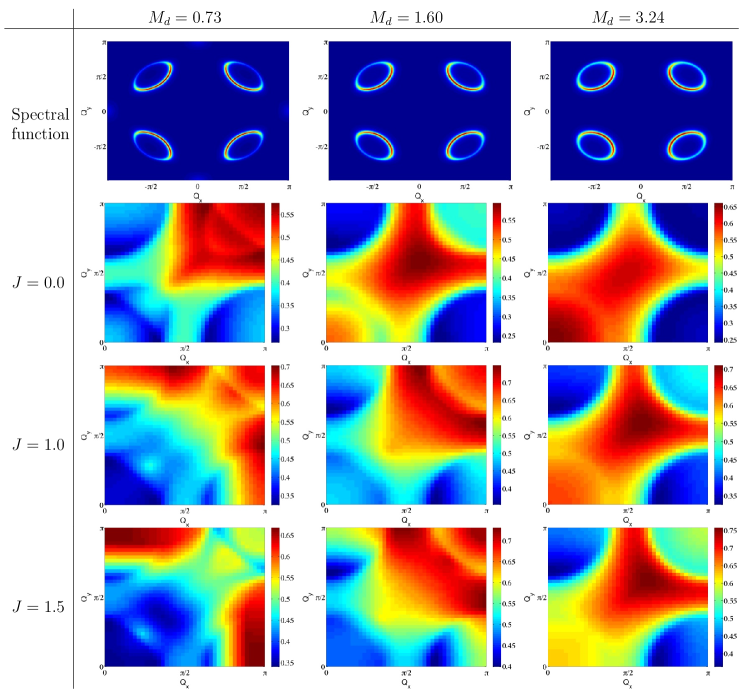
Fig. 6 shows the spectral functions and minimum eigenvalues for Ud+2Jsubscript𝑈𝑑2𝐽U_{d}+2J ranging from 3.25 to 8.0 with the chemical potential chosen so that the hole density p0.10similar-to𝑝0.10p\sim 0.10. The other parameters are given in the bottom row of Table 1.

As is apparent from Fig. 6, the minimal eigenvalues are consistently along the axes either at (±Q1,2,0)plus-or-minussubscript𝑄120(\pm Q_{1,2},0) and (0,±Q1,2)0plus-or-minussubscript𝑄12(0,\pm Q_{1,2}), with Q1π/3subscript𝑄1𝜋3Q_{1}\approx\pi/3 and Q22π/3subscript𝑄22𝜋3Q_{2}\approx 2\pi/3. The orientation of the eigenvalue is therefore in accord with experiments. The global minimum is mostly at the wavevector Q2subscript𝑄2Q_{2}, which corresponds approximately to the distance between the tips of the hole pockets shown in the top row of Fig. 6. In a few cases, there is also a well-formed minimum at Q1subscript𝑄1Q_{1}; we do not have a correspondingly simple interpretation of Q1subscript𝑄1Q_{1}, but suspect that it is related to the incipient electron pocket near the antinodes which is present at smaller magnetic order.

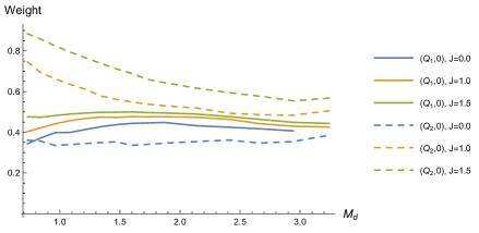
Turning to the form factors, recall our observation above that the eigenmodes have components both in the S=0𝑆0S=0 charge density wave at 𝐐𝐐{\mathbf{Q}} and in the S=1𝑆1S=1 spin density wave at 𝐐+(π,π)𝐐𝜋𝜋{\mathbf{Q}}+(\pi,\pi). We show in Fig. 7 the relative weights of the S=0𝑆0S=0 and S=1𝑆1S=1 components at the wavevectors (Q1,0)subscript𝑄10(Q_{1},0) and (Q2,0)subscript𝑄20(Q_{2},0). For most of the cases, the weight in the spin density wave component is actually dominant. This appears to be due to the proximity of the critical point where the antiferromagnetic order at (π,π)𝜋𝜋(\pi,\pi) vanishes, and amplitude fluctuations in the Néel order are enhanced.

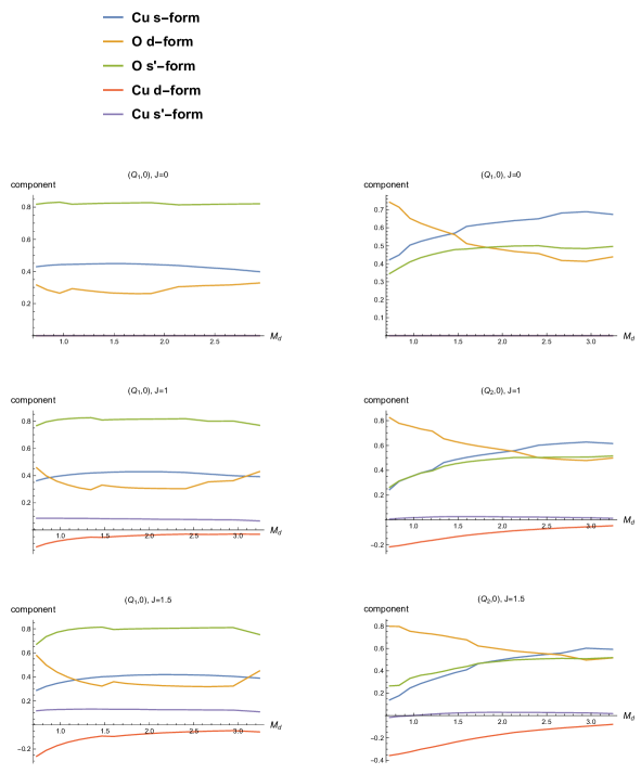
Nonetheless, when we take into account the orientational fluctuations of the Néel order induced by a non-zero temperature, we expect that the S=1𝑆1S=1 components will average to zero . For this reason, we focus on the spatial structure of the S=0𝑆0S=0 component of the order parameter alone. The normalized components of the eigenvector projected into the S=0𝑆0S=0 components are shown in Fig. 8. The consistent trend in these plots, and one of our key results, is that increasing the magnetic order, Mdsubscript𝑀𝑑M_{d}, leads to a decrease in the d𝑑d components and a corresponding increase in the ssuperscript𝑠s^{\prime} components.

Refer to caption
Figure 6: (Color online) Spectral functions and minimum eigenvalues for Md=subscript𝑀𝑑absentM_{d}=0.73, 1.60 and 3.24 (which corresponds to Ud+2J=subscript𝑈𝑑2𝐽absentU_{d}+2J= 3.25, 5.0 and 8.0 respectively). The chemical potential is adjusted so that p0.10similar-to𝑝0.10p\sim 0.10, while Vpp=1.5subscript𝑉𝑝𝑝1.5V_{pp}=1.5 and Vpd=1.0subscript𝑉𝑝𝑑1.0V_{pd}=1.0. The second through fourth columns are for J=0.0, 1.0,𝐽0.01.0J=0.0,\,1.0, and 1.51.51.5 respectively. Note that the minimum eigenvalues are mostly at (Q2,0)subscript𝑄20(Q_{2},0) with Q22π/3subscript𝑄22𝜋3Q_{2}\approx 2\pi/3; in some cases there are also well-formed minima at (Q1,0)subscript𝑄10(Q_{1},0) with Q1π/3subscript𝑄1𝜋3Q_{1}\approx\pi/3.
Refer to caption
Figure 7: (Color online) The sum of the squares of the S=0𝑆0S=0 components of the original eigenvectors corresponding to the minimum eigenvalues at (Q1,0)subscript𝑄10(Q_{1},0) and (Q2,0)subscript𝑄20(Q_{2},0). That is, we plot l=123|𝒫l(𝐐)|2superscriptsubscript𝑙123superscriptsubscript𝒫𝑙𝐐2\sum_{l=1}^{23}\left|\mathcal{P}_{l}({\mathbf{Q}})\right|^{2} at 𝐐=(Q1,2,0)𝐐subscript𝑄120{\mathbf{Q}}=(Q_{1,2},0) where {𝒫l(𝐐)}subscript𝒫𝑙𝐐\{\mathcal{P}_{l}({\mathbf{Q}})\} are the components corresponding to the 46 basis functions given in Tables 6 and 7. We subsequently project out the S=1𝑆1S=1 components (l=2446𝑙2446l=24-46) and normalize.
Refer to caption
Figure 8: (Color online) S=0𝑆0S=0 form factor dependence at (Q1,0)subscript𝑄10(Q_{1},0) and (Q2,0)subscript𝑄20(Q_{2},0), as a function of magnetization Mdsubscript𝑀𝑑M_{d} (from which Ud+2Jsubscript𝑈𝑑2𝐽U_{d}+2J is determined). These values are determined by projecting out the S=1𝑆1S=1 components of the eigenvectors and subsequently normalizing. Only the most important contributions are displayed. On the first row, the legend is shown. In descending order the remaining rows show the results for J=0.0, 1.0𝐽0.01.0J=0.0,\,1.0 and 1.51.51.5. The other interaction parameters are given in Table 1 and the chemical potential is chosen so that p0.10similar-to𝑝0.10p\sim 0.10.

IV Conclusions

This paper has analyzed charge ordering instabilities of 3-band models of the cuprates. Consistent with earlier results on related models, we find that starting from a metal with a large Fermi surface invariably leads, in the simplest RPA approximation, to charge-ordering along a ‘diagonal’ wavevector, which disagrees with experimental observations. However, as suggested in Ref. Atkinson et al., 2015, starting from a Fermi surface reconstructed by antiferromagnetic order leads to the observed charge ordering along the principal axes. We examined the form-factors of this ordering, and found that its d𝑑d-wave character was suppressed as the strength of the magnetic order was increased. This trend is consistent with recent X-ray experimental observations of charge order in LBCO in Ref. Achkar et al., 2014, which measured the ratio of ssuperscript𝑠s^{\prime} to d𝑑d components on the O sites. Our results for these parameters are in Fig. 8. The magnetically ordered LBCO compound has a much larger s/dsuperscript𝑠𝑑s^{\prime}/d ratio than that observed by STM in the non-magnetic compounds Fujita et al. (2014).

The model of magnetic order used in the present paper is rather crude, and it would be interesting to extend the computations to more realistic models. We have assumed magnetic order at (π,π)𝜋𝜋(\pi,\pi), whereas the magnetic order in LBCO is incommensurate. The magnetic order has been assumed to be static, but it would be interesting to examine the influence of a frequency-dependent electronic self energy in a Eliashberg framework. This would then complement the spin-liquid perspective taken recently in Ref. Chowdhury and Sachdev, 2014.

Finally, we note that our renormalized classical treatment of magnetic order here is more appropriate for the electron-doped cuprates Kyung et al. (2004). Interestingly, charge order has recently been observed in an electron-doped compound da Silva Neto et al. (2015) with a wavevector which is close to the (±Q1,0)plus-or-minussubscript𝑄10(\pm Q_{1},0) wavevector found in our computations above. It would be interesting to measure the form factor of this ordering: the implication of our results here is that the s𝑠s-form factor will be larger than in the hole-doped cuprates.

Acknowledgments

We thank B. Atkinson, D. Chowdhury, D. Hawthorn, and A. Kampf for useful discussions. This research was supported by the NSF under Grant DMR-1360789, the Templeton foundation, and MURI grant W911NF-14-1-0003 from ARO. Research at Perimeter Institute is supported by the Government of Canada through Industry Canada and by the Province of Ontario through the Ministry of Research and Innovation.

Appendix A Basis functions

This appendix expresses the Hamiltonian in Eq. (9) in Fourier space, and then writes it in terms of basis functions which aid in the determination of the eigenmodes in the particle-hole sector. We begin by introducing the Fourier transforms

cdα(𝐫i)subscript𝑐𝑑𝛼subscript𝐫𝑖\displaystyle c_{d\alpha}({\mathbf{r}}_{i}) =𝐤ei𝐤𝐫icdα(𝐤),absentsubscript𝐤superscript𝑒𝑖𝐤subscript𝐫𝑖subscript𝑐𝑑𝛼𝐤\displaystyle=\sum_{\mathbf{k}}e^{-i{\mathbf{k}}\cdot{\mathbf{r}}_{i}}c_{d\alpha}({\mathbf{k}}), cdα(𝐫i)subscriptsuperscript𝑐𝑑𝛼subscript𝐫𝑖\displaystyle c^{\dagger}_{d\alpha}({\mathbf{r}}_{i}) =𝐤ei𝐤𝐫icdα(𝐤)absentsubscript𝐤superscript𝑒𝑖𝐤subscript𝐫𝑖subscriptsuperscript𝑐𝑑𝛼𝐤\displaystyle=\sum_{\mathbf{k}}e^{i{\mathbf{k}}\cdot{\mathbf{r}}_{i}}c^{\dagger}_{d\alpha}({\mathbf{k}}) (26)
cμα(𝐫i)subscript𝑐𝜇𝛼subscript𝐫𝑖\displaystyle c_{\mu\alpha}({\mathbf{r}}_{i}) =i𝐤ei𝐤(𝐫i+𝐑μ)cμα(𝐤),absent𝑖subscript𝐤superscript𝑒𝑖𝐤subscript𝐫𝑖subscript𝐑𝜇subscript𝑐𝜇𝛼𝐤\displaystyle=-i\sum_{\mathbf{k}}e^{-i{\mathbf{k}}\cdot({\mathbf{r}}_{i}+\mathbf{R}_{\mu})}c_{\mu\alpha}({\mathbf{k}}), cμα(𝐫i)subscriptsuperscript𝑐𝜇𝛼subscript𝐫𝑖\displaystyle c^{\dagger}_{\mu\alpha}({\mathbf{r}}_{i}) =i𝐤ei𝐤(𝐫i+𝐑μ)cμα(𝐤)absent𝑖subscript𝐤superscript𝑒𝑖𝐤subscript𝐫𝑖subscript𝐑𝜇subscriptsuperscript𝑐𝜇𝛼𝐤\displaystyle=i\sum_{\mathbf{k}}e^{i{\mathbf{k}}\cdot({\mathbf{r}}_{i}+\mathbf{R}_{\mu})}c^{\dagger}_{\mu\alpha}({\mathbf{k}}) μ=x,y𝜇𝑥𝑦\displaystyle\mu=x,y

where 𝐑μsubscript𝐑𝜇\mathbf{R}_{\mu} is the position within the unit cell of the μ𝜇\muth orbital: 𝐑d=0subscript𝐑𝑑0\mathbf{R}_{d}=0, 𝐑x=+𝐱^/2subscript𝐑𝑥^𝐱2\mathbf{R}_{x}=+\hat{\mathbf{x}}/2, and 𝐑y=+𝐲^/2subscript𝐑𝑦^𝐲2\mathbf{R}_{y}=+\hat{\mathbf{y}}/2. The Coulomb terms become

H^Ch=𝐤,𝐤,𝐪superscriptsubscript^𝐻𝐶subscript𝐤superscript𝐤𝐪\displaystyle\hat{H}_{C}^{h}=\sum_{{\mathbf{k}},{\mathbf{k}}^{\prime},{\mathbf{q}}} [Udcd(𝐤𝐪/2)cd(𝐤𝐪/2)cd(𝐤+𝐪/2)cd(𝐤+𝐪/2)\displaystyle\bigg{[}U_{d}\,c_{d\uparrow}^{\dagger}({\mathbf{k}}^{\prime}-{\mathbf{q}}/2)c_{d\uparrow}({\mathbf{k}}-{\mathbf{q}}/2)c_{d\downarrow}^{\dagger}({\mathbf{k}}+{\mathbf{q}}/2)c_{d\downarrow}({\mathbf{k}}^{\prime}+{\mathbf{q}}/2) (27)
+Up(cx(𝐤𝐪/2)cx(𝐤𝐪/2)cx(𝐤+𝐪/2)cx(𝐤+𝐪/2)\displaystyle+U_{p}\bigg{(}c_{x\uparrow}^{\dagger}({\mathbf{k}}^{\prime}-{\mathbf{q}}/2)c_{x\uparrow}({\mathbf{k}}-{\mathbf{q}}/2)c_{x\downarrow}^{\dagger}({\mathbf{k}}+{\mathbf{q}}/2)c_{x\downarrow}({\mathbf{k}}^{\prime}+{\mathbf{q}}/2)
+cy(𝐤𝐪/2)cy(𝐤𝐪/2)cy(𝐤+𝐪/2)cy(𝐤+𝐪/2))]\displaystyle\phantom{+U_{p}\bigg{(}}+c_{y\uparrow}^{\dagger}({\mathbf{k}}^{\prime}-{\mathbf{q}}/2)c_{y\uparrow}({\mathbf{k}}-{\mathbf{q}}/2)c_{y\downarrow}^{\dagger}({\mathbf{k}}+{\mathbf{q}}/2)c_{y\downarrow}({\mathbf{k}}^{\prime}+{\mathbf{q}}/2)\bigg{)}\bigg{]}
H^Cv=𝐤,𝐤,𝐪superscriptsubscript^𝐻𝐶𝑣subscript𝐤superscript𝐤𝐪\displaystyle\hat{H}_{C}^{v}=\sum_{{\mathbf{k}},{\mathbf{k}}^{\prime},{\mathbf{q}}} [2Vpd(cos(kxkx2)cdα(𝐤𝐪/2)cdα(𝐤𝐪/2)cxβ(𝐤+𝐪/2)cxβ(𝐤+𝐪/2)\displaystyle\bigg{[}2V_{pd}\bigg{(}\cos\left({k_{x}-k_{x}^{\prime}\over 2}\right)c_{d\alpha}^{\dagger}({\mathbf{k}}^{\prime}-{\mathbf{q}}/2)c_{d\alpha}({\mathbf{k}}-{\mathbf{q}}/2)c_{x{\beta}}^{\dagger}({\mathbf{k}}+{\mathbf{q}}/2)c_{x{\beta}}({\mathbf{k}}^{\prime}+{\mathbf{q}}/2) (28)
+cos(kyky2)cdα(𝐤𝐪/2)cdα(𝐤𝐪/2)cyβ(𝐤+𝐪/2)cyβ(𝐤+𝐪/2))\displaystyle+\cos\left({k_{y}-k_{y}^{\prime}\over 2}\right)c_{d\alpha}^{\dagger}({\mathbf{k}}^{\prime}-{\mathbf{q}}/2)c_{d\alpha}({\mathbf{k}}-{\mathbf{q}}/2)c_{y{\beta}}^{\dagger}({\mathbf{k}}+{\mathbf{q}}/2)c_{y{\beta}}({\mathbf{k}}^{\prime}+{\mathbf{q}}/2)\bigg{)}
+4Vppcos(kxkx2)cos(kyky2)cxα(𝐤𝐪/2)cxα(𝐤𝐪/2)cyβ(𝐤+𝐪/2)cyβ(𝐤+𝐪/2)]\displaystyle+4V_{pp}\cos\left({k_{x}-k_{x}^{\prime}\over 2}\right)\cos\left({k_{y}-k_{y}^{\prime}\over 2}\right)c_{x\alpha}^{\dagger}({\mathbf{k}}^{\prime}-{\mathbf{q}}/2)c_{x\alpha}({\mathbf{k}}-{\mathbf{q}}/2)c_{y{\beta}}^{\dagger}({\mathbf{k}}+{\mathbf{q}}/2)c_{y{\beta}}({\mathbf{k}}^{\prime}+{\mathbf{q}}/2)\bigg{]}

and the copper-copper exchange interaction is given by

H^J=𝐤,𝐤,𝐪aJ4(cos(kxkx)+cos(kyky))cdα(𝐤𝐪/2)σαβacdβ(𝐤𝐪/2)cdγ(𝐤+𝐪/2)σγδacdδ(𝐤+𝐪/2).subscript^𝐻𝐽subscript𝐤superscript𝐤𝐪subscript𝑎𝐽4subscript𝑘𝑥superscriptsubscript𝑘𝑥subscript𝑘𝑦superscriptsubscript𝑘𝑦subscriptsuperscript𝑐𝑑𝛼superscript𝐤𝐪2subscriptsuperscript𝜎𝑎𝛼𝛽subscript𝑐𝑑𝛽𝐤𝐪2subscriptsuperscript𝑐𝑑𝛾𝐤𝐪2subscriptsuperscript𝜎𝑎𝛾𝛿subscript𝑐𝑑𝛿superscript𝐤𝐪2\displaystyle\hat{H}_{J}=\sum_{{\mathbf{k}},{\mathbf{k}}^{\prime},{\mathbf{q}}}\sum_{a}{J\over 4}\left(\cos(k_{x}-k_{x}^{\prime})+\cos(k_{y}-k_{y}^{\prime})\right)c^{\dagger}_{d\alpha}({\mathbf{k}}^{\prime}-{\mathbf{q}}/2)\sigma^{a}_{\alpha{\beta}}c_{d{\beta}}({\mathbf{k}}-{\mathbf{q}}/2)c^{\dagger}_{d\gamma}({\mathbf{k}}+{\mathbf{q}}/2)\sigma^{a}_{\gamma\delta}c_{d\delta}({\mathbf{k}}^{\prime}+{\mathbf{q}}/2)\,. (29)

These expressions may be simplified by writing them as a sum over the basis functions ϕμνl(𝐤)subscriptsuperscriptitalic-ϕ𝑙𝜇𝜈𝐤\phi^{\,l}_{\mu\nu}({\mathbf{k}}) given in Table 3.

l𝑙l μ𝜇\mu ν𝜈\nu ϕμνl(𝐤)subscriptsuperscriptitalic-ϕ𝑙𝜇𝜈𝐤\phi^{\,l}_{\mu\nu}({\mathbf{k}})
1 d𝑑d d𝑑d δμdδνdsubscript𝛿𝜇𝑑subscript𝛿𝜈𝑑\delta_{\mu d}\,\delta_{\nu d}
2 x𝑥x x𝑥x δμxδνxsubscript𝛿𝜇𝑥subscript𝛿𝜈𝑥\delta_{\mu x}\,\delta_{\nu x}
3 y𝑦y y𝑦y δμyδνysubscript𝛿𝜇𝑦subscript𝛿𝜈𝑦\delta_{\mu y}\,\delta_{\nu y}
4 d𝑑d x𝑥x δμdδνx2cos(kx2)subscript𝛿𝜇𝑑subscript𝛿𝜈𝑥2subscript𝑘𝑥2\delta_{\mu d}\,\delta_{\nu x}\sqrt{2}\cos\left({k_{x}\over 2}\right)
5 x𝑥x d𝑑d δμxδνd2cos(kx2)subscript𝛿𝜇𝑥subscript𝛿𝜈𝑑2subscript𝑘𝑥2\delta_{\mu x}\,\delta_{\nu d}\sqrt{2}\cos\left({k_{x}\over 2}\right)
6 d𝑑d x𝑥x δμdδνx2sin(kx2)subscript𝛿𝜇𝑑subscript𝛿𝜈𝑥2subscript𝑘𝑥2\delta_{\mu d}\,\delta_{\nu x}\sqrt{2}\sin\left({k_{x}\over 2}\right)
7 x𝑥x d𝑑d δμxδνd2sin(kx2)subscript𝛿𝜇𝑥subscript𝛿𝜈𝑑2subscript𝑘𝑥2\delta_{\mu x}\,\delta_{\nu d}\sqrt{2}\sin\left({k_{x}\over 2}\right)
8 d𝑑d y𝑦y δμdδνy2cos(ky2)subscript𝛿𝜇𝑑subscript𝛿𝜈𝑦2subscript𝑘𝑦2\delta_{\mu d}\,\delta_{\nu y}\sqrt{2}\cos\left({k_{y}\over 2}\right)
9 y𝑦y d𝑑d δμyδνd2cos(ky2)subscript𝛿𝜇𝑦subscript𝛿𝜈𝑑2subscript𝑘𝑦2\delta_{\mu y}\,\delta_{\nu d}\sqrt{2}\cos\left({k_{y}\over 2}\right)
10 d𝑑d y𝑦y δμdδνy2sin(ky2)subscript𝛿𝜇𝑑subscript𝛿𝜈𝑦2subscript𝑘𝑦2\delta_{\mu d}\,\delta_{\nu y}\sqrt{2}\sin\left({k_{y}\over 2}\right)
11 y𝑦y d𝑑d δμyδνd2sin(ky2)subscript𝛿𝜇𝑦subscript𝛿𝜈𝑑2subscript𝑘𝑦2\delta_{\mu y}\,\delta_{\nu d}\sqrt{2}\sin\left({k_{y}\over 2}\right)
l𝑙l μ𝜇\mu ν𝜈\nu ϕμνl(𝐤)subscriptsuperscriptitalic-ϕ𝑙𝜇𝜈𝐤\phi^{\,l}_{\mu\nu}({\mathbf{k}})
12 x𝑥x y𝑦y δμxδνy 2cos(kx2)cos(ky2)subscript𝛿𝜇𝑥subscript𝛿𝜈𝑦2subscript𝑘𝑥2subscript𝑘𝑦2\delta_{\mu x}\,\delta_{\nu y}\,2\cos\left({k_{x}\over 2}\right)\cos\left({k_{y}\over 2}\right)
13 y𝑦y x𝑥x δμyδνx 2cos(kx2)cos(ky2)subscript𝛿𝜇𝑦subscript𝛿𝜈𝑥2subscript𝑘𝑥2subscript𝑘𝑦2\delta_{\mu y}\,\delta_{\nu x}\,2\cos\left({k_{x}\over 2}\right)\cos\left({k_{y}\over 2}\right)
14 x𝑥x y𝑦y δμxδνy 2cos(kx2)sin(ky2)subscript𝛿𝜇𝑥subscript𝛿𝜈𝑦2subscript𝑘𝑥2subscript𝑘𝑦2\delta_{\mu x}\,\delta_{\nu y}\,2\cos\left({k_{x}\over 2}\right)\sin\left({k_{y}\over 2}\right)
15 y𝑦y x𝑥x δμyδνx 2cos(kx2)sin(ky2)subscript𝛿𝜇𝑦subscript𝛿𝜈𝑥2subscript𝑘𝑥2subscript𝑘𝑦2\delta_{\mu y}\,\delta_{\nu x}\,2\cos\left({k_{x}\over 2}\right)\sin\left({k_{y}\over 2}\right)
16 x𝑥x y𝑦y δμxδνy 2sin(kx2)cos(ky2)subscript𝛿𝜇𝑥subscript𝛿𝜈𝑦2subscript𝑘𝑥2subscript𝑘𝑦2\delta_{\mu x}\,\delta_{\nu y}\,2\sin\left({k_{x}\over 2}\right)\cos\left({k_{y}\over 2}\right)
17 y𝑦y x𝑥x δμyδνx 2sin(kx2)cos(ky2)subscript𝛿𝜇𝑦subscript𝛿𝜈𝑥2subscript𝑘𝑥2subscript𝑘𝑦2\delta_{\mu y}\,\delta_{\nu x}\,2\sin\left({k_{x}\over 2}\right)\cos\left({k_{y}\over 2}\right)
18 x𝑥x y𝑦y δμxδνy 2sin(kx2)sin(ky2)subscript𝛿𝜇𝑥subscript𝛿𝜈𝑦2subscript𝑘𝑥2subscript𝑘𝑦2\delta_{\mu x}\,\delta_{\nu y}\,2\sin\left({k_{x}\over 2}\right)\sin\left({k_{y}\over 2}\right)
19 y𝑦y x𝑥x δμyδνx 2sin(kx2)sin(ky2)subscript𝛿𝜇𝑦subscript𝛿𝜈𝑥2subscript𝑘𝑥2subscript𝑘𝑦2\delta_{\mu y}\,\delta_{\nu x}\,2\sin\left({k_{x}\over 2}\right)\sin\left({k_{y}\over 2}\right)
20 d𝑑d d𝑑d δμdδνd(coskxcosky)subscript𝛿𝜇𝑑subscript𝛿𝜈𝑑subscript𝑘𝑥subscript𝑘𝑦\delta_{\mu d}\,\delta_{\nu d}\left(\cos{k_{x}}-\cos k_{y}\right)
21 d𝑑d d𝑑d δμdδνd(coskx+cosky)subscript𝛿𝜇𝑑subscript𝛿𝜈𝑑subscript𝑘𝑥subscript𝑘𝑦\delta_{\mu d}\,\delta_{\nu d}\left(\cos{k_{x}}+\cos k_{y}\right)
22 d𝑑d d𝑑d δμdδνd(sinkxsinky)subscript𝛿𝜇𝑑subscript𝛿𝜈𝑑subscript𝑘𝑥subscript𝑘𝑦\delta_{\mu d}\,\delta_{\nu d}\left(\sin{k_{x}}-\sin k_{y}\right)
23 d𝑑d d𝑑d δμdδνd(sinkx+sinky)subscript𝛿𝜇𝑑subscript𝛿𝜈𝑑subscript𝑘𝑥subscript𝑘𝑦\delta_{\mu d}\,\delta_{\nu d}\left(\sin{k_{x}}+\sin k_{y}\right)
Table 3: For each l𝑙l-index, ϕμνl(𝐤)subscriptsuperscriptitalic-ϕ𝑙𝜇𝜈𝐤\phi^{l}_{\mu\nu}({\mathbf{k}}) is nonzero only for the μνlimit-from𝜇𝜈\mu\nu-pair given in the second and third columns of each table. The full function is shown in the fourth column.

In this basis, the interaction Hamiltonian becomes

H^C+H^J=𝐤,𝐤,𝐪[\displaystyle\hat{H}_{C}+\hat{H}_{J}=\sum_{{\mathbf{k}},{\mathbf{k}}^{\prime},{\mathbf{q}}}\bigg{[} l=119μν𝒱l2ϕμνl(𝐤)ϕμνl(𝐤)cμα(𝐤𝐪/2)cμα(𝐤𝐪/2)cνβ(𝐤+𝐪/2)cνβ(𝐤+𝐪/2)superscriptsubscript𝑙119subscript𝜇𝜈subscript𝒱𝑙2subscriptsuperscriptitalic-ϕ𝑙𝜇𝜈𝐤subscriptsuperscriptitalic-ϕ𝑙𝜇𝜈superscript𝐤subscriptsuperscript𝑐𝜇𝛼superscript𝐤𝐪2subscript𝑐𝜇𝛼𝐤𝐪2subscriptsuperscript𝑐𝜈𝛽𝐤𝐪2subscript𝑐𝜈𝛽superscript𝐤𝐪2\displaystyle\sum_{l=1}^{19}\sum_{\mu\nu}{\mathcal{V}_{l}\over 2}\phi^{\,l}_{\mu\nu}({\mathbf{k}}){\phi^{\,l}_{\mu\nu}({\mathbf{k}}^{\prime})}c^{\dagger}_{\mu\alpha}({\mathbf{k}}^{\prime}-{\mathbf{q}}/2)c_{\mu\alpha}({\mathbf{k}}-{\mathbf{q}}/2)c^{\dagger}_{\nu{\beta}}({\mathbf{k}}+{\mathbf{q}}/2)c_{\nu{\beta}}({\mathbf{k}}^{\prime}+{\mathbf{q}}/2) (30)
+l=2023μν𝒱l6ϕμνl(𝐤)ϕμνl(𝐤)cdα(𝐤𝐪/2)σαβacdβ(𝐤𝐪/2)cdγ(𝐤+𝐪/2)σγδacdδ(𝐤+𝐪/2)].\displaystyle+\sum_{l=20}^{23}\sum_{\mu\nu}{\mathcal{V}_{l}\over 6}\phi^{\,l}_{\mu\nu}({\mathbf{k}}){\phi^{\,l}_{\mu\nu}({\mathbf{k}}^{\prime})}c^{\dagger}_{d\alpha}({\mathbf{k}}^{\prime}-{\mathbf{q}}/2)\sigma^{a}_{\alpha{\beta}}c_{d{\beta}}({\mathbf{k}}-{\mathbf{q}}/2)c^{\dagger}_{d\gamma}({\mathbf{k}}+{\mathbf{q}}/2)\sigma^{a}_{\gamma\delta}c_{d\delta}({\mathbf{k}}^{\prime}+{\mathbf{q}}/2)\bigg{]}\,.

where the interaction parameters 𝒱lsubscript𝒱𝑙\mathcal{V}_{l} are given by

𝒱l={Ud,l=1Up,l=2, 3Vpd,l=411Vpp,l=12193J/4,l=2023.\displaystyle\mathcal{V}_{l}=\left\{\begin{matrix}[l]U_{d},&l=1\\ U_{p},&l=2,\,3\\ V_{pd},&l=4-11\\ V_{pp},&l=12-19\\ 3J/4,&l=20-23\end{matrix}\right.\,. (31)

The action of time-reversal on the basis functions is summarized in Table 4.

l𝑙l μ𝜇\mu ν𝜈\nu 𝒯𝒫l(𝐐)𝒯subscript𝒫𝑙𝐐\mathcal{T}\mathcal{P}_{l}({\mathbf{Q}})
1 d𝑑d d𝑑d 𝒯:𝒫1(𝐐):𝒯subscript𝒫1𝐐\mathcal{T}:\mathcal{P}_{1}({\mathbf{Q}}) maps-to\mapsto 𝒫1(𝐐)subscript𝒫1𝐐\phantom{-}\mathcal{P}_{1}({\mathbf{Q}})
2 x𝑥x x𝑥x 𝒯:𝒫2(𝐐):𝒯subscript𝒫2𝐐\mathcal{T}:\mathcal{P}_{2}({\mathbf{Q}}) maps-to\mapsto 𝒫2(𝐐)subscript𝒫2𝐐\phantom{-}\mathcal{P}_{2}({\mathbf{Q}})
3 y𝑦y y𝑦y 𝒯:𝒫3(𝐐):𝒯subscript𝒫3𝐐\mathcal{T}:\mathcal{P}_{3}({\mathbf{Q}}) maps-to\mapsto 𝒫3(𝐐)subscript𝒫3𝐐\phantom{-}\mathcal{P}_{3}({\mathbf{Q}})
4 d𝑑d x𝑥x 𝒯:𝒫4(𝐐):𝒯subscript𝒫4𝐐\mathcal{T}:\mathcal{P}_{4}({\mathbf{Q}}) maps-to\mapsto 𝒫5(𝐐)subscript𝒫5𝐐-\mathcal{P}_{5}({\mathbf{Q}})
5 x𝑥x d𝑑d 𝒯:𝒫5(𝐐):𝒯subscript𝒫5𝐐\mathcal{T}:\mathcal{P}_{5}({\mathbf{Q}}) maps-to\mapsto 𝒫4(𝐐)subscript𝒫4𝐐-\mathcal{P}_{4}({\mathbf{Q}})
6 d𝑑d x𝑥x 𝒯:𝒫6(𝐐):𝒯subscript𝒫6𝐐\mathcal{T}:\mathcal{P}_{6}({\mathbf{Q}}) maps-to\mapsto 𝒫7(𝐐)subscript𝒫7𝐐\phantom{-}\mathcal{P}_{7}({\mathbf{Q}})
7 x𝑥x d𝑑d 𝒯:𝒫7(𝐐):𝒯subscript𝒫7𝐐\mathcal{T}:\mathcal{P}_{7}({\mathbf{Q}}) maps-to\mapsto 𝒫6(𝐐)subscript𝒫6𝐐\phantom{-}\mathcal{P}_{6}({\mathbf{Q}})
8 d𝑑d y𝑦y 𝒯:𝒫8(𝐐):𝒯subscript𝒫8𝐐\mathcal{T}:\mathcal{P}_{8}({\mathbf{Q}}) maps-to\mapsto 𝒫9(𝐐)subscript𝒫9𝐐-\mathcal{P}_{9}({\mathbf{Q}})
9 y𝑦y d𝑑d 𝒯:𝒫9(𝐐):𝒯subscript𝒫9𝐐\mathcal{T}:\mathcal{P}_{9}({\mathbf{Q}}) maps-to\mapsto 𝒫8(𝐐)subscript𝒫8𝐐-\mathcal{P}_{8}({\mathbf{Q}})
10 d𝑑d y𝑦y 𝒯:𝒫10(𝐐):𝒯subscript𝒫10𝐐\mathcal{T}:\mathcal{P}_{10}({\mathbf{Q}}) maps-to\mapsto 𝒫11(𝐐)subscript𝒫11𝐐\phantom{-}\mathcal{P}_{11}({\mathbf{Q}})
11 y𝑦y d𝑑d 𝒯:𝒫11(𝐐):𝒯subscript𝒫11𝐐\mathcal{T}:\mathcal{P}_{11}({\mathbf{Q}}) maps-to\mapsto 𝒫10(𝐐)subscript𝒫10𝐐\phantom{-}\mathcal{P}_{10}({\mathbf{Q}})
l𝑙l μ𝜇\mu ν𝜈\nu 𝒯𝒫l(𝐐)𝒯subscript𝒫𝑙𝐐\mathcal{T}\mathcal{P}_{l}({\mathbf{Q}})
12 x𝑥x y𝑦y 𝒯:𝒫12(𝐐):𝒯subscript𝒫12𝐐\mathcal{T}:\mathcal{P}_{12}({\mathbf{Q}}) maps-to\mapsto 𝒫13(𝐐)subscript𝒫13𝐐\phantom{-}\mathcal{P}_{13}({\mathbf{Q}})
13 y𝑦y x𝑥x 𝒯:𝒫13(𝐐):𝒯subscript𝒫13𝐐\mathcal{T}:\mathcal{P}_{13}({\mathbf{Q}}) maps-to\mapsto 𝒫12(𝐐)subscript𝒫12𝐐\phantom{-}\mathcal{P}_{12}({\mathbf{Q}})
14 x𝑥x y𝑦y 𝒯:𝒫14(𝐐):𝒯subscript𝒫14𝐐\mathcal{T}:\mathcal{P}_{14}({\mathbf{Q}}) maps-to\mapsto 𝒫15(𝐐)subscript𝒫15𝐐-\mathcal{P}_{15}({\mathbf{Q}})
15 y𝑦y x𝑥x 𝒯:𝒫15(𝐐):𝒯subscript𝒫15𝐐\mathcal{T}:\mathcal{P}_{15}({\mathbf{Q}}) maps-to\mapsto 𝒫14(𝐐)subscript𝒫14𝐐-\mathcal{P}_{14}({\mathbf{Q}})
16 x𝑥x y𝑦y 𝒯:𝒫16(𝐐):𝒯subscript𝒫16𝐐\mathcal{T}:\mathcal{P}_{16}({\mathbf{Q}}) maps-to\mapsto 𝒫17(𝐐)subscript𝒫17𝐐-\mathcal{P}_{17}({\mathbf{Q}})
17 y𝑦y x𝑥x 𝒯:𝒫17(𝐐):𝒯subscript𝒫17𝐐\mathcal{T}:\mathcal{P}_{17}({\mathbf{Q}}) maps-to\mapsto 𝒫16(𝐐)subscript𝒫16𝐐-\mathcal{P}_{16}({\mathbf{Q}})
18 x𝑥x y𝑦y 𝒯:𝒫18(𝐐):𝒯subscript𝒫18𝐐\mathcal{T}:\mathcal{P}_{18}({\mathbf{Q}}) maps-to\mapsto 𝒫19(𝐐)subscript𝒫19𝐐\phantom{-}\mathcal{P}_{19}({\mathbf{Q}})
19 y𝑦y x𝑥x 𝒯:𝒫19(𝐐):𝒯subscript𝒫19𝐐\mathcal{T}:\mathcal{P}_{19}({\mathbf{Q}}) maps-to\mapsto 𝒫18(𝐐)subscript𝒫18𝐐\phantom{-}\mathcal{P}_{18}({\mathbf{Q}})
20 d𝑑d d𝑑d 𝒯:𝒫20(𝐐):𝒯subscript𝒫20𝐐\mathcal{T}:\mathcal{P}_{20}({\mathbf{Q}}) maps-to\mapsto 𝒫20(𝐐)subscript𝒫20𝐐\phantom{-}\mathcal{P}_{20}({\mathbf{Q}})
21 d𝑑d d𝑑d 𝒯:𝒫21(𝐐):𝒯subscript𝒫21𝐐\mathcal{T}:\mathcal{P}_{21}({\mathbf{Q}}) maps-to\mapsto 𝒫21(𝐐)subscript𝒫21𝐐\phantom{-}\mathcal{P}_{21}({\mathbf{Q}})
22 d𝑑d d𝑑d 𝒯:𝒫22(𝐐):𝒯subscript𝒫22𝐐\mathcal{T}:\mathcal{P}_{22}({\mathbf{Q}}) maps-to\mapsto 𝒫22(𝐐)subscript𝒫22𝐐-\mathcal{P}_{22}({\mathbf{Q}})
23 d𝑑d d𝑑d 𝒯:𝒫23(𝐐):𝒯subscript𝒫23𝐐\mathcal{T}:\mathcal{P}_{23}({\mathbf{Q}}) maps-to\mapsto 𝒫23(𝐐)subscript𝒫23𝐐-\mathcal{P}_{23}({\mathbf{Q}})
Table 4: The actions of time-reversal on the basis function coefficients {𝒫l(𝐤)}subscript𝒫𝑙𝐤\{\mathcal{P}_{l}({\mathbf{k}})\}.

Since the eigenvectors corresponding to the lowest eigenvalues are in general time-reversal preserving, we focus on this case. Table 5 summarizes the relationship between the real-space order parameter Pijμνsuperscriptsubscript𝑃𝑖𝑗𝜇𝜈P_{ij}^{\mu\nu} and an eigenvector {𝒫l(𝐐)}subscript𝒫𝑙𝐐\{\mathcal{P}_{l}({\mathbf{Q}})\}. Note that the amplitude is multiplied by the sign of the hopping term in the Hamiltonian corresponding to that bond has. Fig. 9 gives these signs and shows how these look on the lattice.

Bond Definitions Pijμνsuperscriptsubscript𝑃𝑖𝑗𝜇𝜈P_{ij}^{\mu\nu}
𝒫1cos(𝐐𝐫i)δi,jsubscript𝒫1𝐐subscript𝐫𝑖subscript𝛿𝑖𝑗\mathcal{P}_{1}\cos\left({\mathbf{Q}}\cdot{\mathbf{r}}_{i}\right)\delta_{i,j}
dd𝑑𝑑dd Rddxsuperscriptsubscript𝑅𝑑𝑑𝑥R_{dd}^{x} = (𝒫20+𝒫21)/2subscript𝒫20subscript𝒫212\left(-\mathcal{P}_{20}+\mathcal{P}_{21}\right)/2 +Rddx[cos(𝐐𝐫i+Qx2)δi,j𝐱^+R^{x}_{dd}\,\big{[}\cos\left({\mathbf{Q}}\cdot{\mathbf{r}}_{i}+{Q_{x}\over 2}\right)\delta_{i,j-\hat{\mathbf{x}}}
Rddysuperscriptsubscript𝑅𝑑𝑑𝑦R_{dd}^{y} = (𝒫20+𝒫21)/2subscript𝒫20subscript𝒫212\left(\mathcal{P}_{20}+\mathcal{P}_{21}\right)/2 +cos(𝐐𝐫iQx2)δi,j+𝐱^]\phantom{R_{dd}^{x}\big{[}}+\cos\left({\mathbf{Q}}\cdot{\mathbf{r}}_{i}-{Q_{x}\over 2}\right)\delta_{i,j+\hat{\mathbf{x}}}\big{]}
+Rddy[cos(𝐐𝐫i+Qy2)δi,j𝐲^+R_{dd}^{y}\big{[}\cos\left({\mathbf{Q}}\cdot{\mathbf{r}}_{i}+{Q_{y}\over 2}\right)\delta_{i,j-\hat{\mathbf{y}}}
+cos(𝐐𝐫iQy2)δi,j+𝐲^]\phantom{R^{y}_{dd}\big{[}}+\cos\left({\mathbf{Q}}\cdot{\mathbf{r}}_{i}-{Q_{y}\over 2}\right)\delta_{i,j+\hat{\mathbf{y}}}\big{]}
xx𝑥𝑥xx 𝒫2cos(𝐐𝐫i+Qx2)δi,jsubscript𝒫2𝐐subscript𝐫𝑖subscript𝑄𝑥2subscript𝛿𝑖𝑗\mathcal{P}_{2}\cos\left({\mathbf{Q}}\cdot{\mathbf{r}}_{i}+{Q_{x}\over 2}\right)\delta_{i,j}
yy𝑦𝑦yy 𝒫3cos(𝐐𝐫i+Qy2)δi,jsubscript𝒫3𝐐subscript𝐫𝑖subscript𝑄𝑦2subscript𝛿𝑖𝑗\mathcal{P}_{3}\cos\left({\mathbf{Q}}\cdot{\mathbf{r}}_{i}+{Q_{y}\over 2}\right)\delta_{i,j}
dx𝑑𝑥dx Rdxsubscript𝑅𝑑𝑥R_{dx} == (𝒫42+𝒫62)/2superscriptsubscript𝒫42superscriptsubscript𝒫622\sqrt{\left(\mathcal{P}_{4}^{2}+\mathcal{P}_{6}^{2}\right)/2} Rdx[cos(𝐐𝐫i+Qx4+θdx)δi,j{R_{dx}}\Big{[}\cos\left({\mathbf{Q}}\cdot{\mathbf{r}}_{i}+{Q_{x}\over 4}+\theta_{dx}\right)\delta_{i,j}
θdxsubscript𝜃𝑑𝑥\theta_{dx} == arctan(𝒫4/𝒫6)subscript𝒫4subscript𝒫6\arctan\left({\mathcal{P}_{4}/\mathcal{P}_{6}}\right) +cos(𝐐𝐫iQx4θdx)δi,j+𝐱^]\phantom{R2}+\cos\left({\mathbf{Q}}\cdot{\mathbf{r}}_{i}-{Q_{x}\over 4}-\theta_{dx}\right)\delta_{i,j+\hat{\mathbf{x}}}\Big{]}
dy𝑑𝑦dy Rdysubscript𝑅𝑑𝑦R_{dy} == (𝒫82+𝒫102)/2superscriptsubscript𝒫82superscriptsubscript𝒫1022\sqrt{\left(\mathcal{P}_{8}^{2}+\mathcal{P}_{10}^{2}\right)/2} Rdy[cos(𝐐𝐫i+Qy4+θdy)δi,j{R_{dy}}\Big{[}-\cos\left({\mathbf{Q}}\cdot{\mathbf{r}}_{i}+{Q_{y}\over 4}+\theta_{dy}\right)\delta_{i,j}
θdysubscript𝜃𝑑𝑦\theta_{dy} == arctan(𝒫8/𝒫10)subscript𝒫8subscript𝒫10\arctan\left({\mathcal{P}_{8}/\mathcal{P}_{10}}\right) cos(𝐐𝐫iQy4θdy)δi,j+𝐲^]\phantom{R_{dy}\big{[}}-\cos\left({\mathbf{Q}}\cdot{\mathbf{r}}_{i}-{Q_{y}\over 4}-\theta_{dy}\right)\delta_{i,j+\hat{\mathbf{y}}}\Big{]}
xy𝑥𝑦xy Rxysuperscriptsubscript𝑅𝑥𝑦R_{xy}^{-} == 12(𝒫12𝒫18)2+(𝒫14+𝒫16)212superscriptsubscript𝒫12subscript𝒫182superscriptsubscript𝒫14subscript𝒫162{1\over 2}\sqrt{\left(\mathcal{P}_{12}-\mathcal{P}_{18}\right)^{2}+\left(\mathcal{P}_{14}+\mathcal{P}_{16}\right)^{2}} +Rxy[cos(𝐐𝐫i+Qx4Qy4+θxy)δi,j+𝐲^+{R_{xy}^{-}}\Big{[}\cos\left({\mathbf{Q}}\cdot{\mathbf{r}}_{i}+{Q_{x}\over 4}-{Q_{y}\over 4}+\theta_{xy}^{-}\right)\delta_{i,j+\hat{\mathbf{y}}}
θxysuperscriptsubscript𝜃𝑥𝑦\theta_{xy}^{-} == arctan[(𝒫14+𝒫16)/(𝒫12𝒫18)]subscript𝒫14subscript𝒫16subscript𝒫12subscript𝒫18\arctan\big{[}\left(\mathcal{P}_{14}+\mathcal{P}_{16}\right)/\left(\mathcal{P}_{12}-\mathcal{P}_{18}\right)\big{]} +cos(𝐐𝐫i+3Qx4+Qy4θxy)δi,j𝐱^]\phantom{{R_{xy}^{-}\over 2}}\,+\cos\left({\mathbf{Q}}\cdot{\mathbf{r}}_{i}+{3Q_{x}\over 4}+{Q_{y}\over 4}-\theta_{xy}^{-}\right)\delta_{i,j-\hat{\mathbf{x}}}\Big{]}
Rxy+superscriptsubscript𝑅𝑥𝑦R_{xy}^{+} == 12(𝒫12+𝒫18)2+(𝒫14+𝒫16)212superscriptsubscript𝒫12subscript𝒫182superscriptsubscript𝒫14subscript𝒫162{1\over 2}\sqrt{\left(\mathcal{P}_{12}+\mathcal{P}_{18}\right)^{2}+\left(-\mathcal{P}_{14}+\mathcal{P}_{16}\right)^{2}} Rxy+[cos(𝐐𝐫i+Qx4+Qy4+θxy+)δi,j-{R_{xy}^{+}}\Big{[}\cos\left({\mathbf{Q}}\cdot{\mathbf{r}}_{i}+{Q_{x}\over 4}+{Q_{y}\over 4}+\theta_{xy}^{+}\right)\delta_{i,j}
θxy+superscriptsubscript𝜃𝑥𝑦\theta_{xy}^{+} == arctan[(𝒫14+𝒫16)/(𝒫12+𝒫18)]subscript𝒫14subscript𝒫16subscript𝒫12subscript𝒫18\arctan\big{[}\left(-\mathcal{P}_{14}+\mathcal{P}_{16}\right)/\left(\mathcal{P}_{12}+\mathcal{P}_{18}\right)\big{]} +cos(𝐐𝐫i+3Qx4Qy4θxy+)δi,j𝐱^+𝐲^]\phantom{{R_{xy}^{-}\over 2}}\,+\cos\left({\mathbf{Q}}\cdot{\mathbf{r}}_{i}+{3Q_{x}\over 4}-{Q_{y}\over 4}-\theta_{xy}^{+}\right)\delta_{i,j-\hat{\mathbf{x}}+\hat{\mathbf{y}}}\Big{]}
Table 5: Transition amplitudes in the time-reversal invariant sector at wave vector 𝐐𝐐{\mathbf{Q}}.
Refer to caption
Figure 9: Real space representation of hopping amplitudes. The signs written in the dx𝑑𝑥dx, dy𝑑𝑦dy, and xy𝑥𝑦xy bonds in (b) and (c) indicate which sign the hopping term in the Hamiltonian corresponding to that bond has. The amplitudes given in Table 5 have been multiplied by this phase.

Appendix B Basis functions with antiferromagnetic order

To determine the momentum space representation of the Hamiltonian in the presence of antiferromagnetic order in Eq. (25), we begin by introducing a new electron operator ψμσsubscript𝜓𝜇𝜎\psi_{\mu\sigma} :

ψμ(𝐤)subscript𝜓𝜇absent𝐤\displaystyle\psi_{\mu\uparrow}({\mathbf{k}}) =cμ(𝐤)absentsubscript𝑐𝜇absent𝐤\displaystyle=c_{\mu\uparrow}({\mathbf{k}}) ψμ(𝐤)subscript𝜓𝜇absent𝐤\displaystyle\psi_{\mu\downarrow}({\mathbf{k}}) =cμ(𝐤+𝐊).absentsubscript𝑐𝜇absent𝐤𝐊\displaystyle=c_{\mu\downarrow}({\mathbf{k}}+{\mathbf{K}})\,. (32)

With these operators we re-express Eq. 25 as

H^AF=𝐤[\displaystyle\hat{H}_{AF}=-\sum_{\mathbf{k}}\Bigg{[} Md(ψd(𝐤)ψd(𝐤)+h.c.)\displaystyle M_{d}\left(\psi_{d\uparrow}^{\dagger}({\mathbf{k}})\psi_{d\downarrow}({\mathbf{k}})+h.c.\right) (33)
+2Mpd(cos(kx2)ψd(𝐤)ψx(𝐤+𝐊)+sin(kx2)ψx(𝐤)ψd(𝐤)+h.c.\displaystyle+2M_{pd}\Big{(}-\cos\left({k_{x}\over 2}\right)\psi_{d\uparrow}^{\dagger}({\mathbf{k}})\psi_{x\downarrow}({\mathbf{k}}+{\mathbf{K}})+\sin\left({k_{x}\over 2}\right)\psi_{x\uparrow}^{\dagger}({\mathbf{k}})\psi_{d\downarrow}({\mathbf{k}})+h.c.
+cos(ky2)ψd(𝐤)ψy(𝐤+𝐊)sin(ky2)ψy(𝐤)ψd(𝐤)+h.c.)\displaystyle\phantom{M_{pd}\Bigg{(}}+\cos\left({k_{y}\over 2}\right)\psi_{d\uparrow}^{\dagger}({\mathbf{k}})\psi_{y\downarrow}({\mathbf{k}}+{\mathbf{K}})-\sin\left({k_{y}\over 2}\right)\psi_{y\uparrow}^{\dagger}({\mathbf{k}})\psi_{d\downarrow}({\mathbf{k}})+h.c.\Big{)}
+4Mpp(sin(kx2)cos(ky2)ψx(𝐤)ψy(𝐤)\displaystyle+4M_{pp}\Big{(}\sin\left({k_{x}\over 2}\right)\cos\left({k_{y}\over 2}\right)\psi_{x\uparrow}^{\dagger}({\mathbf{k}})\psi_{y\downarrow}({\mathbf{k}})
+cos(kx2)sin(ky2)ψy(𝐤)ψx(𝐤)+h.c.)].\displaystyle\phantom{+4M_{pp}\Big{(}}+\cos\left({k_{x}\over 2}\right)\sin\left({k_{y}\over 2}\right)\psi_{y\uparrow}^{\dagger}({\mathbf{k}})\psi_{x\downarrow}({\mathbf{k}})+h.c.\Big{)}\Bigg{]}\,.

The full hopping hamiltonian is now

H^tsuperscriptsubscript^𝐻𝑡\displaystyle{\hat{H}}_{t}^{\prime} =𝐤Ψ𝐤(𝐤)Ψ𝐤,absentsubscript𝐤superscriptsubscriptΨ𝐤𝐤subscriptΨ𝐤\displaystyle=\sum_{\mathbf{k}}{\Psi}_{\mathbf{k}}^{\dagger}{\mathcal{H}}({\mathbf{k}}){\Psi}_{\mathbf{k}}, Ψ𝐤superscriptsubscriptΨ𝐤\displaystyle{\Psi}_{{\mathbf{k}}}^{\dagger} =(ψd(𝐤),ψx(𝐤),ψy(𝐤),ψd(𝐤),ψx(𝐤),ψy(𝐤))absentsuperscriptsubscript𝜓𝑑absent𝐤superscriptsubscript𝜓𝑥absent𝐤superscriptsubscript𝜓𝑦absent𝐤superscriptsubscript𝜓𝑑absent𝐤superscriptsubscript𝜓𝑥absent𝐤superscriptsubscript𝜓𝑦absent𝐤\displaystyle=\left(\psi_{d\uparrow}^{\dagger}({\mathbf{k}}),\psi_{x\uparrow}^{\dagger}({\mathbf{k}}),\psi_{y\uparrow}^{\dagger}({\mathbf{k}}),\psi_{d\downarrow}^{\dagger}({\mathbf{k}}),\psi_{x\downarrow}^{\dagger}({\mathbf{k}}),\psi_{y\downarrow}^{\dagger}({\mathbf{k}})\right) (34)
(𝐤)𝐤\displaystyle{\mathcal{H}}({\mathbf{k}}) =((𝐤)𝐌(𝐤)𝐌(𝐤)(𝐤+𝐊))absentmatrix𝐤subscript𝐌absent𝐤subscript𝐌absent𝐤𝐤𝐊\displaystyle=\begin{pmatrix}\mathcal{H}({\mathbf{k}})&-\mathbf{M}_{\uparrow\downarrow}({\mathbf{k}})\\ -\mathbf{M}_{\downarrow\uparrow}({\mathbf{k}})&\mathcal{H}({\mathbf{k}}+{\mathbf{K}})\end{pmatrix} (35)

where

𝐌(𝐤)subscript𝐌absent𝐤\displaystyle\mathbf{M}_{\uparrow\downarrow}({\mathbf{k}}) =(Md2Mpdcos(kx2)2Mpdcos(ky2)2Mpdsin(kx2)04Mppsin(kx2)cos(ky2)2Mpdsin(ky2)4Mppcos(kx2)sin(ky2)0)absentmatrixsubscript𝑀𝑑2subscript𝑀𝑝𝑑subscript𝑘𝑥22subscript𝑀𝑝𝑑subscript𝑘𝑦22subscript𝑀𝑝𝑑subscript𝑘𝑥204subscript𝑀𝑝𝑝subscript𝑘𝑥2subscript𝑘𝑦22subscript𝑀𝑝𝑑subscript𝑘𝑦24subscript𝑀𝑝𝑝subscript𝑘𝑥2subscript𝑘𝑦20\displaystyle=\begin{pmatrix}M_{d}&-2M_{pd}\cos\left({k_{x}\over 2}\right)&2M_{pd}\cos\left({k_{y}\over 2}\right)\\ 2M_{pd}\sin\left({k_{x}\over 2}\right)&0&4M_{pp}\sin\left({k_{x}\over 2}\right)\cos\left({k_{y}\over 2}\right)\\ -2M_{pd}\sin\left({k_{y}\over 2}\right)&4M_{pp}\cos\left({k_{x}\over 2}\right)\sin\left({k_{y}\over 2}\right)&0\end{pmatrix} (36)
𝐌(𝐤)subscript𝐌absent𝐤\displaystyle\mathbf{M}_{\downarrow\uparrow}({\mathbf{k}}) =(Md2Mpdsin(kx2)2Mpdsin(ky2)2Mpdcos(kx2)04Mppcos(kx2)sin(ky2)2Mpdcos(ky2)4Mppsin(kx2)cos(ky2)0).absentmatrixsubscript𝑀𝑑2subscript𝑀𝑝𝑑subscript𝑘𝑥22subscript𝑀𝑝𝑑subscript𝑘𝑦22subscript𝑀𝑝𝑑subscript𝑘𝑥204subscript𝑀𝑝𝑝subscript𝑘𝑥2subscript𝑘𝑦22subscript𝑀𝑝𝑑subscript𝑘𝑦24subscript𝑀𝑝𝑝subscript𝑘𝑥2subscript𝑘𝑦20\displaystyle=\begin{pmatrix}M_{d}&-2M_{pd}\sin\left({k_{x}\over 2}\right)&2M_{pd}\sin\left({k_{y}\over 2}\right)\\ 2M_{pd}\cos\left({k_{x}\over 2}\right)&0&4M_{pp}\cos\left({k_{x}\over 2}\right)\sin\left({k_{y}\over 2}\right)\\ -2M_{pd}\cos\left({k_{y}\over 2}\right)&4M_{pp}\sin\left({k_{x}\over 2}\right)\cos\left({k_{y}\over 2}\right)&0\end{pmatrix}. (37)

In order to determine the parameters Mdsubscript𝑀𝑑M_{d}, Mpdsubscript𝑀𝑝𝑑M_{pd}, and Mppsubscript𝑀𝑝𝑝M_{pp}, we must solve the following mean-field equations:

Mdsubscript𝑀𝑑\displaystyle M_{d} =(Ud+2J)𝐤cd(𝐤)cd(𝐤+𝐊)absentsubscript𝑈𝑑2𝐽subscript𝐤expectationsuperscriptsubscript𝑐𝑑absent𝐤subscript𝑐𝑑absent𝐤𝐊\displaystyle=\left(U_{d}+2J\right)\sum_{\mathbf{k}}\Braket{c_{d\uparrow}^{\dagger}({\mathbf{k}})c_{d\downarrow}({\mathbf{k}}+{\mathbf{K}})} (38)
Mpdsubscript𝑀𝑝𝑑\displaystyle M_{pd} =Vpd𝐤sin(kx2)cd(𝐤)cx(𝐤+𝐊)absentsubscript𝑉𝑝𝑑subscript𝐤subscript𝑘𝑥2expectationsuperscriptsubscript𝑐𝑑absent𝐤subscript𝑐𝑥absent𝐤𝐊\displaystyle=V_{pd}\sum_{\mathbf{k}}\sin\left({k_{x}\over 2}\right)\Braket{c_{d\uparrow}^{\dagger}({\mathbf{k}})c_{x\downarrow}({\mathbf{k}}+{\mathbf{K}})}
Mppsubscript𝑀𝑝𝑝\displaystyle M_{pp} =Vpp𝐤sin(kx2)cos(ky2)cx(𝐤)cy(𝐤+𝐊).absentsubscript𝑉𝑝𝑝subscript𝐤subscript𝑘𝑥2subscript𝑘𝑦2expectationsuperscriptsubscript𝑐𝑥absent𝐤subscript𝑐𝑦absent𝐤𝐊\displaystyle=V_{pp}\sum_{\mathbf{k}}\sin\left({k_{x}\over 2}\right)\cos\left({k_{y}\over 2}\right)\Braket{c_{x\uparrow}^{\dagger}({\mathbf{k}})c_{y\downarrow}({\mathbf{k}}+{\mathbf{K}})}\,.

As discussed in Section II.1, the presence of AF order, will mix the charge and spin channels. Naively, it follows that the number of basis functions needed will increase by a factor of four since they must now carry spin indices as well. Using the original basis functions in Table 3, we define

φμν,σσl(𝐤)={δσδσϕμνl(𝐤),l=123δσδσϕμνl23(𝐤),l=2446δσδσϕμνl46(𝐤),l=4769δσδσϕμνl69(𝐤),l=7092.\displaystyle{\varphi}_{\mu\nu,\sigma\sigma^{\prime}}^{l}({\mathbf{k}})=\left\{\begin{matrix}[l]\delta_{\sigma\uparrow}\delta_{\sigma^{\prime}\uparrow}\,\phi^{l}_{\mu\nu}({\mathbf{k}}),&l=1-23\\ \delta_{\sigma\downarrow}\delta_{\sigma^{\prime}\downarrow}\,\phi^{\,l-23}_{\mu\nu}({\mathbf{k}}),&l=24-46\\ \delta_{\sigma\uparrow}\delta_{\sigma^{\prime}\downarrow}\,\phi^{\,l-46}_{\mu\nu}({\mathbf{k}}),&l=47-69\\ \delta_{\sigma\downarrow}\delta_{\sigma^{\prime}\uparrow}\,\phi^{\,l-69}_{\mu\nu}({\mathbf{k}}),&l=70-92\end{matrix}\right.\,. (39)

Alternatively, we can simply write φμν,σσl(𝐤)=φabl(𝐤)subscriptsuperscript𝜑𝑙𝜇𝜈𝜎superscript𝜎𝐤subscriptsuperscript𝜑𝑙𝑎𝑏𝐤{\varphi}^{l}_{\mu\nu,\sigma\sigma^{\prime}}({\mathbf{k}})=\varphi^{l}_{ab}({\mathbf{k}}) where a=(μ,σ)𝑎𝜇𝜎a=(\mu,\sigma) and b=(ν,σ)𝑏𝜈superscript𝜎b=(\nu,\sigma^{\prime}). In this basis, the interaction Hamiltonian is

H^int=subscript^𝐻𝑖𝑛𝑡absent\displaystyle\hat{H}_{int}= 𝐪,𝐤,𝐤[l,m1μναβ𝒱l2φμν,αβl(𝐤)φμν,αβm(𝐤)ψμα(𝐤𝐪/2)ψμα(𝐤𝐪/2)ψνβ(𝐤+𝐪/2)ψνβ(𝐤+𝐪/2)\displaystyle\sum_{{\mathbf{q}},{\mathbf{k}},{\mathbf{k}}^{\prime}}\Bigg{[}\sum_{l,m\in\mathcal{I}^{1}}\sum_{\mu\nu}\sum_{\alpha{\beta}}{{\mathcal{V}}_{l}\over 2}{{\varphi}}^{\,l}_{\mu\nu,\alpha{\beta}}({\mathbf{k}}){{\varphi}}^{\,m}_{\mu\nu,\alpha{\beta}}({\mathbf{k}}^{\prime})\psi^{\dagger}_{\mu\alpha}({\mathbf{k}}^{\prime}-{\mathbf{q}}/2)\psi_{\mu\alpha}({\mathbf{k}}-{\mathbf{q}}/2)\psi^{\dagger}_{\nu{\beta}}({\mathbf{k}}+{\mathbf{q}}/2)\psi_{\nu{\beta}}({\mathbf{k}}^{\prime}+{\mathbf{q}}/2) (40)
+l,mJ𝒥l2(αβφdd,αβl(𝐤)φdd,αβm(𝐤)(ψdα(𝐤𝐪/2)σααzψdα(𝐤𝐪/2)ψdβ(𝐤+𝐪/2)σββzψdβ(𝐤+𝐪/2)\displaystyle+\sum_{l,m\in\mathcal{I}^{J}}{\mathcal{J}_{l}\over 2}\bigg{(}\sum_{\begin{subarray}{c}\alpha{\beta}\end{subarray}}\,{{\varphi}}^{\,l}_{dd,\alpha{\beta}}({\mathbf{k}}){{\varphi}}^{\,m}_{dd,\alpha{\beta}}({\mathbf{k}}^{\prime})\big{(}\psi^{\dagger}_{d\alpha}({\mathbf{k}}^{\prime}-{\mathbf{q}}/2)\sigma^{z}_{\alpha\alpha}\psi_{d\alpha}({\mathbf{k}}-{\mathbf{q}}/2)\psi^{\dagger}_{d{\beta}}({\mathbf{k}}+{\mathbf{q}}/2)\sigma^{z}_{{\beta}{\beta}}\psi_{d{\beta}}({\mathbf{k}}^{\prime}+{\mathbf{q}}/2)
2φdd,l(𝐤)φdd,m(𝐤)ψd(𝐤𝐪/2)ψd(𝐤𝐪/2)ψd(𝐤+𝐪/2)ψd(𝐤+𝐪/2)2subscriptsuperscript𝜑𝑙𝑑𝑑absent𝐤subscriptsuperscript𝜑𝑚𝑑𝑑absentsuperscript𝐤subscriptsuperscript𝜓𝑑absentsuperscript𝐤𝐪2subscript𝜓𝑑absent𝐤𝐪2subscriptsuperscript𝜓𝑑absent𝐤𝐪2subscript𝜓𝑑absentsuperscript𝐤𝐪2\displaystyle\phantom{+\sum_{l,m\in\mathcal{I}^{J}}\mathcal{V}_{l}\bigg{(}}-2{{\varphi}}^{\,l}_{dd,\downarrow\downarrow}({\mathbf{k}}){{\varphi}}^{\,m}_{dd,\uparrow\uparrow}({\mathbf{k}}^{\prime})\psi^{\dagger}_{d\uparrow}({\mathbf{k}}^{\prime}-{\mathbf{q}}/2)\psi_{d\downarrow}({\mathbf{k}}-{\mathbf{q}}/2)\psi^{\dagger}_{d\downarrow}({\mathbf{k}}+{\mathbf{q}}/2)\psi_{d\uparrow}({\mathbf{k}}^{\prime}+{\mathbf{q}}/2)
2φdd,l(𝐤)φdd,m(𝐤)ψd(𝐤𝐪/2)ψd(𝐤𝐪/2)ψd(𝐤+𝐪/2)ψd(𝐤+𝐪/2))].\displaystyle\phantom{+\sum_{l,m\in\mathcal{I}^{J}}\mathcal{V}_{l}\bigg{(}}-2{{\varphi}}^{\,l}_{dd,\uparrow\uparrow}({\mathbf{k}}){{\varphi}}^{\,m}_{dd,\downarrow\downarrow}({\mathbf{k}}^{\prime})\psi^{\dagger}_{d\downarrow}({\mathbf{k}}^{\prime}-{\mathbf{q}}/2)\psi_{d\uparrow}({\mathbf{k}}-{\mathbf{q}}/2)\psi^{\dagger}_{d\uparrow}({\mathbf{k}}+{\mathbf{q}}/2)\psi_{d\downarrow}({\mathbf{k}}^{\prime}+{\mathbf{q}}/2)\bigg{)}\Bigg{]}\,.

where 1={119,2442,4765,7088}superscript1119244247657088\mathcal{I}^{1}=\{1-19,24-42,47-65,70-88\} and J={2023,4346,6669,8992}superscript𝐽2023434666698992\mathcal{I}^{J}=\{20-23,43-46,66-69,89-92\}. The parameters 𝒱lsubscript𝒱𝑙\mathcal{V}_{l} are given by

𝒱lsubscript𝒱𝑙\displaystyle\mathcal{V}_{l} ={𝒱l,l=123𝒱l23,l=2446𝒱l46,l=4769𝒱l69,l=7092\displaystyle=\left\{\begin{matrix}[l]\mathcal{V}_{l}^{\prime},&l=1-23\\ \mathcal{V}_{l-23}^{\prime},&l=24-46\\ \mathcal{V}_{l-46}^{\prime},&l=47-69\\ \mathcal{V}_{l-69}^{\prime},&l=70-92\end{matrix}\right. 𝒱lsuperscriptsubscript𝒱𝑙\displaystyle\mathcal{V}_{l}^{\prime} ={Ud,l=1Up,l=2,3Vpd,l=411Vpp,l=12190,otherwise.\displaystyle=\left\{\begin{matrix}[l]U_{d},&l=1\\ U_{p},&l=2,3\\ V_{pd},&l=4-11\\ V_{pp},&l=12-19\\ 0,&\text{otherwise}\end{matrix}\right.\,. (41)

and the Cu-Cu exchange interaction strength is simply

𝒥lsubscript𝒥𝑙\displaystyle\mathcal{J}_{l} ={𝒥l,l=123𝒥l23,l=2446𝒥l46,l=4769𝒥l69,l=7092\displaystyle=\left\{\begin{matrix}[l]\mathcal{J}_{l}^{\prime},&l=1-23\\ \mathcal{J}_{l-23}^{\prime},&l=24-46\\ \mathcal{J}_{l-46}^{\prime},&l=47-69\\ \mathcal{J}_{l-69}^{\prime},&l=70-92\end{matrix}\right. 𝒥lsubscriptsuperscript𝒥𝑙\displaystyle\mathcal{J}^{\prime}_{l} ={J/4,l=10,otherwise.\displaystyle=\left\{\begin{matrix}[l]J/4,&l=1\\ 0,&\text{otherwise}\end{matrix}\right.\,. (42)

Appendix C T𝑇T-Matrix Solutions in the presence of AF order

Here we reproduce the calculation of Section II.1 in the presence of AF order. As above, the interaction vertex may be separated into an exchange and a direct part. It is given by

𝐕μμ,νναα,ββ(𝐤,𝐤;𝐪)subscriptsuperscript𝐕𝛼superscript𝛼𝛽superscript𝛽𝜇superscript𝜇𝜈superscript𝜈𝐤superscript𝐤𝐪\displaystyle{\mathbf{V}}^{\alpha\alpha^{\prime},{\beta}{\beta}^{\prime}}_{\mu\mu^{\prime},\nu\nu^{\prime}}({\mathbf{k}},{\mathbf{k}}^{\prime};{\mathbf{q}}) =𝐗μμ,νναα,ββ(𝐤𝐤)𝐖μμ,νναα,ββ(𝐪)absentsubscriptsuperscript𝐗𝛼superscript𝛼𝛽superscript𝛽𝜇superscript𝜇𝜈superscript𝜈𝐤superscript𝐤subscriptsuperscript𝐖𝛼superscript𝛼𝛽superscript𝛽𝜇superscript𝜇𝜈superscript𝜈𝐪\displaystyle={\mathbf{X}}^{\alpha\alpha^{\prime},{\beta}{\beta}^{\prime}}_{\mu\mu^{\prime},\nu\nu^{\prime}}({\mathbf{k}}-{\mathbf{k}}^{\prime})-{\mathbf{W}}^{\alpha\alpha^{\prime},{\beta}{\beta}^{\prime}}_{\mu\mu^{\prime},\nu\nu^{\prime}}({\mathbf{q}}) (43)
=lmφμν,αβl(𝐤)(XlmWlm(𝐪))φμν,αβm(𝐤).absentsubscript𝑙𝑚subscriptsuperscript𝜑𝑙𝜇superscript𝜈𝛼superscript𝛽𝐤subscript𝑋𝑙𝑚subscript𝑊𝑙𝑚𝐪subscriptsuperscript𝜑𝑚superscript𝜇𝜈superscript𝛼𝛽superscript𝐤\displaystyle=\sum_{lm}{\varphi}^{l}_{\mu\nu^{\prime},\alpha{\beta}^{\prime}}({\mathbf{k}})\left({X}_{lm}-{W}_{lm}({\mathbf{q}})\right){\varphi}^{m}_{\mu^{\prime}\nu,\alpha^{\prime}{\beta}}({\mathbf{k}}^{\prime})\,.

To take the different nontrivial spin behaviour into account, we will further separate both the exchange and direct vertices into a J=0𝐽0J=0 and a J0𝐽0J\neq 0 part.

Starting with the exchange vertex, we write 𝐗=𝐗𝟏+𝐗J𝐗superscript𝐗1superscript𝐗𝐽\mathbf{X}=\mathbf{X^{1}}+\mathbf{X}^{J}. The J=0𝐽0J=0 part is given by

𝐗1=𝓧1(𝟙0000𝟙0000𝟙0000𝟙)superscript𝐗1superscript𝓧1matrix1000010000100001\displaystyle\mathbf{X}^{1}=\bm{\mathcal{X}}^{1}\begin{pmatrix}\mathds{1}&0&0&0\\ 0&\mathds{1}&0&0\\ 0&0&\mathds{1}&0\\ 0&0&0&\mathds{1}\\ \end{pmatrix} (44)

where 𝒳𝒳\mathcal{X} is a 23×23232323\times 23 diagonal matrix with elements 𝒳lm1=δlm𝒱lsubscriptsuperscript𝒳1𝑙𝑚subscript𝛿𝑙𝑚superscriptsubscript𝒱𝑙\mathcal{X}^{1}_{lm}=\delta_{lm}\mathcal{V}_{l}^{\prime} with 𝒱lsubscriptsuperscript𝒱𝑙\mathcal{V}^{\prime}_{l} given in Eq. (41). The Cu-Cu exchange term is more complicated, since it depends on the incoming and outgoing spin:

𝐗J=𝓧J(𝟙2𝟙002𝟙𝟙0000𝟙0000𝟙)superscript𝐗𝐽superscript𝓧𝐽matrix121002110000100001\displaystyle\mathbf{X}^{J}=\bm{\mathcal{X}}^{J}\begin{pmatrix}[r]\mathds{1}&-2\mathds{1}&0&0\phantom{-}\\ -2\mathds{1}&\mathds{1}&0&0\phantom{-}\\ 0&0&-\mathds{1}&0\phantom{-}\\ 0&0&0&-\mathds{1}\phantom{-}\end{pmatrix} (45)

where 𝓧Jsuperscript𝓧𝐽\bm{\mathcal{X}}^{J} is a 23×23232323\times 23 diagonal matrix with elements 𝒳lmJ=δlm𝒥lsuperscriptsubscript𝒳𝑙𝑚𝐽subscript𝛿𝑙𝑚superscriptsubscript𝒥𝑙\mathcal{X}_{lm}^{J}=\delta_{lm}\mathcal{J}_{l}^{\prime} with 𝒥lsuperscriptsubscript𝒥𝑙\mathcal{J}_{l}^{\prime} given in Eq. (42). Adding these terms, the total exchange interaction is

𝐗=(𝓧1+𝓧J2𝓧J002𝓧J𝓧1+𝓧J0000𝓧1𝓧J0000𝓧1𝓧J)𝐗matrixsuperscript𝓧1superscript𝓧𝐽2superscript𝓧𝐽002superscript𝓧𝐽superscript𝓧1superscript𝓧𝐽0000superscript𝓧1superscript𝓧𝐽0000superscript𝓧1superscript𝓧𝐽\displaystyle\mathbf{X}=\begin{pmatrix}\bm{\mathcal{X}}^{1}+\bm{\mathcal{X}}^{J}&-2\bm{\mathcal{X}}^{J}&0&0\\ -2\bm{\mathcal{X}}^{J}&\bm{\mathcal{X}}^{1}+\bm{\mathcal{X}}^{J}&0&0\\ 0&0&\bm{\mathcal{X}}^{1}-\bm{\mathcal{X}}^{J}&0\\ 0&0&0&\bm{\mathcal{X}}^{1}-\bm{\mathcal{X}}^{J}\end{pmatrix} (46)

We similarly separate the direct part into a J=0𝐽0J=0 and a J0𝐽0J\neq 0 part:

𝐖(𝐪)=𝐖1(𝐪)+𝐖J(𝐪).𝐖𝐪superscript𝐖1𝐪superscript𝐖𝐽𝐪\displaystyle\mathbf{W}({\mathbf{q}})=\mathbf{W}^{1}({\mathbf{q}})+\mathbf{W}^{J}({\mathbf{q}})\,. (47)

The J=0𝐽0J=0 part is given by

𝐖1(𝐪)=𝓦1(𝐪)(𝟙𝟙00𝟙𝟙0000000000)superscript𝐖1𝐪superscript𝓦1𝐪matrix1100110000000000\displaystyle\mathbf{W}^{1}({\mathbf{q}})=\bm{\mathcal{W}}^{1}({\mathbf{q}})\begin{pmatrix}\mathds{1}&\mathds{1}&0&0\\ \mathds{1}&\mathds{1}&0&0\\ 0&0&0&0\\ 0&0&0&0\end{pmatrix} (48)

where 𝓦1(𝐪)superscript𝓦1𝐪\bm{\mathcal{W}}^{1}({\mathbf{q}}) is the same 23×23232323\times 23 matrix that was used in the case without AFM: 𝒲lm1=0subscriptsuperscript𝒲1𝑙𝑚0\mathcal{W}^{1}_{lm}=0 for l,m>3𝑙𝑚3l,m>3 and for l,m3𝑙𝑚3l,m\leq 3 is given by

𝒲lm1(𝐪)=(Ud2Vpdcos(qx/2)2Vpdcos(qy/2)2Vpdcos(qx/2)Up4Vppcos(qx/2)cos(qy/2)2Vpdcos(qy/2)4Vppcos(qx/2)cos(qy/2)Up)lm.subscriptsuperscript𝒲1𝑙𝑚𝐪subscriptmatrixsubscript𝑈𝑑2subscript𝑉𝑝𝑑subscript𝑞𝑥22subscript𝑉𝑝𝑑subscript𝑞𝑦22subscript𝑉𝑝𝑑subscript𝑞𝑥2subscript𝑈𝑝4subscript𝑉𝑝𝑝subscript𝑞𝑥2subscript𝑞𝑦22subscript𝑉𝑝𝑑subscript𝑞𝑦24subscript𝑉𝑝𝑝subscript𝑞𝑥2subscript𝑞𝑦2subscript𝑈𝑝𝑙𝑚\displaystyle\mathcal{W}^{1}_{lm}({\mathbf{q}})=\begin{pmatrix}U_{d}&2V_{pd}\cos(q_{x}/2)&2V_{pd}\cos(q_{y}/2)\\ 2V_{pd}\cos(q_{x}/2)&U_{p}&4V_{pp}\cos(q_{x}/2)\cos(q_{y}/2)\\ 2V_{pd}\cos(q_{y}/2)&4V_{pp}\cos(q_{x}/2)\cos(q_{y}/2)&U_{p}\end{pmatrix}_{lm}\,. (49)

The Cu-Cu exchange part, 𝐖J(𝐪)superscript𝐖𝐽𝐪\mathbf{W}^{J}({\mathbf{q}}), is given by

𝐖J(𝐪)=𝓦J(𝐪)(𝟙𝟙00𝟙𝟙00002𝟙00002𝟙)superscript𝐖𝐽𝐪superscript𝓦𝐽𝐪matrix110011000021000021\displaystyle\mathbf{W}^{J}({\mathbf{q}})=\bm{\mathcal{W}}^{J}({\mathbf{q}})\begin{pmatrix}[r]\mathds{1}&-\mathds{1}&0&0\phantom{-}\\ -\mathds{1}&\mathds{1}&0&0\phantom{-}\\ 0&0&-2\mathds{1}&0\phantom{-}\\ 0&0&0&-2\mathds{1}\phantom{-}\end{pmatrix} (50)

where 𝓦J(𝐪)superscript𝓦𝐽𝐪\bm{\mathcal{W}}^{J}({\mathbf{q}}) is a 23×23232323\times 23 matrix with elements

𝒲lmJ(𝐪)={12J(cosqx+cosqy),(l,m)=(1,1)0,otherwise.\displaystyle\mathcal{W}^{J}_{lm}({\mathbf{q}})=\left\{\begin{matrix}[l]{1\over 2}J\left(\cos q_{x}+\cos q_{y}\right),&(l,m)=(1,1)\\ 0,&\text{otherwise}\end{matrix}\right.\,. (51)

The total direct interaction may thus be written as

𝐖(𝐪)=(𝓦1+𝓦J𝓦1𝓦J00𝓦1𝓦J𝓦1+𝓦J00002𝓦J00002𝓦J)𝐖𝐪matrixsuperscript𝓦1superscript𝓦𝐽superscript𝓦1superscript𝓦𝐽00superscript𝓦1superscript𝓦𝐽superscript𝓦1superscript𝓦𝐽00002superscript𝓦𝐽00002superscript𝓦𝐽\displaystyle\mathbf{W}({\mathbf{q}})=\begin{pmatrix}\bm{\mathcal{W}}^{1}+\bm{\mathcal{W}}^{J}&\bm{\mathcal{W}}^{1}-\bm{\mathcal{W}}^{J}&0&0\\ \bm{\mathcal{W}}^{1}-\bm{\mathcal{W}}^{J}&\bm{\mathcal{W}}^{1}+\bm{\mathcal{W}}^{J}&0&0\\ 0&0&-2\bm{\mathcal{W}}^{J}&0\\ 0&0&0&-2\bm{\mathcal{W}}^{J}\end{pmatrix} (52)

The Green’s functions are given by diagonalizing the hopping Hamiltonian:

𝐒(𝐤)(𝐤)𝐒(𝐤)=𝚲(𝐤)superscript𝐒𝐤𝐤𝐒𝐤𝚲𝐤\displaystyle\mathbf{S}^{\dagger}({\mathbf{k}})\mathcal{H}({\mathbf{k}})\mathbf{S}({\mathbf{k}})=\mathbf{\Lambda}({\mathbf{k}}) (53)

where Λab(𝐤)=δabE𝐤asubscriptΛ𝑎𝑏𝐤subscript𝛿𝑎𝑏subscriptsuperscript𝐸𝑎𝐤{\Lambda}_{ab}({\mathbf{k}})=\delta_{ab}{E}^{a}_{{\mathbf{k}}} gives the band energies and 𝐒(𝐤)𝐒𝐤{\mathbf{S}}({\mathbf{k}}) is a 6×6666\times 6 matrix of eigenvectors. The roman character indices “a𝑎a” indicate the pair (μ,σ)𝜇𝜎(\mu,\sigma). In the diagonal basis, the bare Green’s function is

𝒢a(𝐤;ωn)=1iωn(Ea(𝐤)μ)subscript𝒢𝑎𝐤subscript𝜔𝑛1𝑖subscript𝜔𝑛superscript𝐸𝑎𝐤𝜇\displaystyle\mathcal{G}_{a}({\mathbf{k}};\omega_{n})={-1\over i\omega_{n}-(E^{a}({\mathbf{k}})-\mu)} (54)

and so the Green’s function in the orbital basis is

Gab(𝐤;ωn)=cSac(𝐤)Sbc(𝐤)1iωn(Ec(𝐤)μ).subscript𝐺𝑎𝑏𝐤subscript𝜔𝑛subscript𝑐subscriptsuperscript𝑆𝑎𝑐𝐤subscript𝑆𝑏𝑐𝐤1𝑖subscript𝜔𝑛superscript𝐸𝑐𝐤𝜇\displaystyle G_{ab}({\mathbf{k}};\omega_{n})=-\sum_{c}S^{*}_{ac}({\mathbf{k}})S_{bc}({\mathbf{k}}){1\over i\omega_{n}-(E^{c}({\mathbf{k}})-\mu)}\,. (55)

The full interaction is given by

Γlm(𝐪)subscriptΓ𝑙𝑚𝐪\displaystyle\Gamma_{lm}({\mathbf{q}}) =Vlm(𝐪)+n,s=192aabb𝐩,ωnVln(𝐪)φabn(𝐩)Gbb(𝐪𝐪/2)φabs(𝐩)Gaa(𝐩+𝐪/2)Γsm(𝐪)absentsubscript𝑉𝑙𝑚𝐪superscriptsubscript𝑛𝑠192subscript𝑎superscript𝑎𝑏superscript𝑏subscript𝐩subscript𝜔𝑛subscript𝑉𝑙𝑛𝐪subscriptsuperscript𝜑𝑛𝑎superscript𝑏𝐩subscript𝐺𝑏superscript𝑏𝐪𝐪2superscriptsubscript𝜑superscript𝑎𝑏𝑠𝐩subscript𝐺𝑎superscript𝑎𝐩𝐪2subscriptΓ𝑠𝑚𝐪\displaystyle=V_{lm}({\mathbf{q}})+\sum_{n,s=1}^{92}\sum_{\begin{subarray}{c}aa^{\prime}\\ bb^{\prime}\end{subarray}}\sum_{{\mathbf{p}},\omega_{n}}V_{ln}({\mathbf{q}}){\varphi}^{n}_{ab^{\prime}}({\mathbf{p}})G_{bb^{\prime}}({\mathbf{q}}-{\mathbf{q}}/2){\varphi}_{a^{\prime}b}^{s}({\mathbf{p}})G_{aa^{\prime}}({\mathbf{p}}+{\mathbf{q}}/2)\Gamma_{sm}({\mathbf{q}}) (56)
=Vlm(𝐪)+n,s=192Vln(𝐪)Πns(𝐪)Γsm(𝐪)absentsubscript𝑉𝑙𝑚𝐪superscriptsubscript𝑛𝑠192subscript𝑉𝑙𝑛𝐪subscriptΠ𝑛𝑠𝐪subscriptΓ𝑠𝑚𝐪\displaystyle=V_{lm}({\mathbf{q}})+\sum_{n,s=1}^{92}V_{ln}({\mathbf{q}})\Pi_{ns}({\mathbf{q}})\Gamma_{sm}({\mathbf{q}})

where polarizability is defined as

Πns(𝐪)subscriptΠ𝑛𝑠𝐪\displaystyle\Pi_{ns}({\mathbf{q}}) =aabb𝐩,ωnφabn(𝐩)Gbb(𝐪𝐪/2)φabs(𝐩)Gaa(𝐩+𝐪/2)absentsubscript𝑎superscript𝑎𝑏superscript𝑏subscript𝐩subscript𝜔𝑛subscriptsuperscript𝜑𝑛𝑎superscript𝑏𝐩subscript𝐺𝑏superscript𝑏𝐪𝐪2superscriptsubscript𝜑superscript𝑎𝑏𝑠𝐩subscript𝐺𝑎superscript𝑎𝐩𝐪2\displaystyle=\sum_{\begin{subarray}{c}aa^{\prime}\\ bb^{\prime}\end{subarray}}\sum_{{\mathbf{p}},\omega_{n}}{\varphi}^{n}_{ab^{\prime}}({\mathbf{p}})G_{bb^{\prime}}({\mathbf{q}}-{\mathbf{q}}/2){\varphi}_{a^{\prime}b}^{s}({\mathbf{p}})G_{aa^{\prime}}({\mathbf{p}}+{\mathbf{q}}/2) (57)
=𝐩aabbccφabn(𝐩)φabs(𝐩)cc,𝐩𝐪bbaaf(Ec(𝐩𝐪/2))f(Ec(𝐩+𝐪/2))Ec(𝐩𝐪/2)Ec(𝐩+𝐪/2)absentsubscript𝐩subscript𝑎superscript𝑎𝑏superscript𝑏subscript𝑐superscript𝑐subscriptsuperscript𝜑𝑛𝑎superscript𝑏𝐩superscriptsubscript𝜑superscript𝑎𝑏𝑠𝐩subscriptsuperscript𝑏superscript𝑏𝑎superscript𝑎superscript𝑐𝑐𝐩𝐪𝑓subscript𝐸superscript𝑐𝐩𝐪2𝑓subscript𝐸𝑐𝐩𝐪2subscript𝐸superscript𝑐𝐩𝐪2subscript𝐸𝑐𝐩𝐪2\displaystyle=-\sum_{\mathbf{p}}\sum_{\begin{subarray}{c}aa^{\prime}\\ bb^{\prime}\end{subarray}}\sum_{cc^{\prime}}{\varphi}^{n}_{ab^{\prime}}({\mathbf{p}}){\varphi}_{a^{\prime}b}^{s}({\mathbf{p}})\mathcal{M}^{bb^{\prime}aa^{\prime}}_{c^{\prime}c,{\mathbf{p}}{\mathbf{q}}}{f(E_{c^{\prime}}({\mathbf{p}}-{\mathbf{q}}/2))-f(E_{c}({\mathbf{p}}+{\mathbf{q}}/2))\over E_{c^{\prime}}({\mathbf{p}}-{\mathbf{q}}/2)-E_{c}({\mathbf{p}}+{\mathbf{q}}/2)}

with

cc,𝐩𝐪bbaa=Sbc(𝐩𝐪/2)Sbc(𝐩𝐪/2)Sac(𝐩+𝐪/2)Sac(𝐩+𝐪/2).subscriptsuperscript𝑏superscript𝑏𝑎superscript𝑎superscript𝑐𝑐𝐩𝐪subscriptsuperscript𝑆𝑏superscript𝑐𝐩𝐪2subscript𝑆superscript𝑏superscript𝑐𝐩𝐪2subscriptsuperscript𝑆𝑎𝑐𝐩𝐪2subscript𝑆superscript𝑎𝑐𝐩𝐪2\displaystyle\mathcal{M}^{bb^{\prime}aa^{\prime}}_{c^{\prime}c,{\mathbf{p}}{\mathbf{q}}}=S^{*}_{bc^{\prime}}({\mathbf{p}}-{\mathbf{q}}/2)S_{b^{\prime}c^{\prime}}({\mathbf{p}}-{\mathbf{q}}/2)S^{*}_{ac}({\mathbf{p}}+{\mathbf{q}}/2)S_{a^{\prime}c}({\mathbf{p}}+{\mathbf{q}}/2)\,. (58)

It follows that we seek the minimum eigenvalues and corresponding eigenvectors of

Alm(𝐪)=δlmn,s=192Vlm(𝐪)Πns(𝐪).subscript𝐴𝑙𝑚𝐪subscript𝛿𝑙𝑚superscriptsubscript𝑛𝑠192subscript𝑉𝑙𝑚𝐪subscriptΠ𝑛𝑠𝐪\displaystyle A_{lm}({\mathbf{q}})=\delta_{lm}-\sum_{n,s=1}^{92}V_{lm}({\mathbf{q}})\Pi_{ns}({\mathbf{q}})\,. (59)

Appendix D Symmetries

This appendix discusses the symmetries of our basis functions in the presence of antiferromagnetic order. In particular we have to pay careful attention to the mixing of the charge density wave mode at wavevector 𝐐𝐐{\mathbf{Q}} with spin density wave at wavevector 𝐐+(π,π)𝐐𝜋𝜋{\mathbf{Q}}+(\pi,\pi).

The Hamiltonian commutes with the total x𝑥x spin

Sx=𝐤μ(cμ(𝐤)cμ(𝐤)+cμ(𝐤)cμ(𝐤))subscript𝑆𝑥subscript𝐤subscript𝜇subscriptsuperscript𝑐𝜇absent𝐤subscript𝑐𝜇absent𝐤superscriptsubscript𝑐𝜇absent𝐤subscript𝑐𝜇absent𝐤\displaystyle S_{x}=\sum_{\mathbf{k}}\sum_{\mu}\left(c^{\dagger}_{\mu\uparrow}({\mathbf{k}})c_{\mu\downarrow}({\mathbf{k}})+c_{\mu\downarrow}^{\dagger}({\mathbf{k}})c_{\mu\uparrow}({\mathbf{k}})\right) (60)

and a translation and spin inversion about the z𝑧z-axis:

𝒜:cμ(𝐤)eikx,ycμ(𝐤),cμ(𝐤)eikx,ycμ(𝐤).\displaystyle\mathcal{A}:\quad c_{\mu\uparrow}({\mathbf{k}})\rightarrow e^{ik_{x,y}}c_{\mu\uparrow}({\mathbf{k}}),\qquad c_{\mu\downarrow}({\mathbf{k}})\rightarrow-e^{ik_{x,y}}c_{\mu\downarrow}({\mathbf{k}})\,. (61)

It follows that the Hamiltonian has the following invariant operators carrying momentum 𝐪𝐪{\mathbf{q}}:

𝐤subscript𝐤\displaystyle\sum_{\mathbf{k}} ϕμνl(𝐤)(cμ(𝐤+𝐪/2)cν(𝐤𝐪/2)+cμ(𝐤+𝐪/2)cν(𝐤𝐪/2))subscriptsuperscriptitalic-ϕ𝑙𝜇𝜈𝐤superscriptsubscript𝑐𝜇absent𝐤𝐪2subscript𝑐𝜈absent𝐤𝐪2superscriptsubscript𝑐𝜇absent𝐤𝐪2subscript𝑐𝜈absent𝐤𝐪2\displaystyle\phi^{l}_{\mu\nu}({\mathbf{k}})\left(c_{\mu\uparrow}^{\dagger}({\mathbf{k}}+{\mathbf{q}}/2)c_{\nu\uparrow}({\mathbf{k}}-{\mathbf{q}}/2)+c_{\mu\downarrow}^{\dagger}({\mathbf{k}}+{\mathbf{q}}/2)c_{\nu\downarrow}({\mathbf{k}}-{\mathbf{q}}/2)\right) (62)
𝐤subscript𝐤\displaystyle\sum_{\mathbf{k}} ϕμνl(𝐤)(cμ(𝐤+𝐪/2+𝐊)cν(𝐤𝐪/2)+cμ(𝐤+𝐪/2+𝐊)cν(𝐤𝐪/2)).subscriptsuperscriptitalic-ϕ𝑙𝜇𝜈𝐤superscriptsubscript𝑐𝜇absent𝐤𝐪2𝐊subscript𝑐𝜈absent𝐤𝐪2superscriptsubscript𝑐𝜇absent𝐤𝐪2𝐊subscript𝑐𝜈absent𝐤𝐪2\displaystyle\phi^{l}_{\mu\nu}({\mathbf{k}})\left(c_{\mu\uparrow}^{\dagger}({\mathbf{k}}+{\mathbf{q}}/2+{\mathbf{K}})c_{\nu\downarrow}({\mathbf{k}}-{\mathbf{q}}/2)+c_{\mu\downarrow}^{\dagger}({\mathbf{k}}+{\mathbf{q}}/2+{\mathbf{K}})c_{\nu\uparrow}({\mathbf{k}}-{\mathbf{q}}/2)\right)\,.

In terms of the ψμα(𝐤)subscript𝜓𝜇𝛼𝐤\psi_{\mu\alpha}({\mathbf{k}}) operators defined above, these are written as

𝐤subscript𝐤\displaystyle\sum_{\mathbf{k}} (ϕμνl(𝐤)ψμ(𝐤+𝐪/2)ψν(𝐤𝐪/2)+ϕμνl(𝐤+𝐊)ψμ(𝐤+𝐪/2)ψν(𝐤𝐪/2))subscriptsuperscriptitalic-ϕ𝑙𝜇𝜈𝐤superscriptsubscript𝜓𝜇absent𝐤𝐪2subscript𝜓𝜈absent𝐤𝐪2subscriptsuperscriptitalic-ϕ𝑙𝜇𝜈𝐤𝐊superscriptsubscript𝜓𝜇absent𝐤𝐪2subscript𝜓𝜈absent𝐤𝐪2\displaystyle\left(\phi^{l}_{\mu\nu}({\mathbf{k}})\psi_{\mu\uparrow}^{\dagger}({\mathbf{k}}+{\mathbf{q}}/2)\psi_{\nu\uparrow}({\mathbf{k}}-{\mathbf{q}}/2)+\phi^{l}_{\mu\nu}({\mathbf{k}}+{\mathbf{K}})\psi_{\mu\downarrow}^{\dagger}({\mathbf{k}}+{\mathbf{q}}/2)\psi_{\nu\downarrow}({\mathbf{k}}-{\mathbf{q}}/2)\right) (63)
𝐤subscript𝐤\displaystyle\sum_{\mathbf{k}} (ϕμνl(𝐤+𝐊)e2i𝐊𝐑μψμ(𝐤+𝐪/2)ψν(𝐤𝐪/2)+ϕμνl(𝐤)ψμ(𝐤+𝐪/2)ψν(𝐤𝐪/2)).subscriptsuperscriptitalic-ϕ𝑙𝜇𝜈𝐤𝐊superscript𝑒2𝑖𝐊subscript𝐑𝜇superscriptsubscript𝜓𝜇absent𝐤𝐪2subscript𝜓𝜈absent𝐤𝐪2subscriptsuperscriptitalic-ϕ𝑙𝜇𝜈𝐤superscriptsubscript𝜓𝜇absent𝐤𝐪2subscript𝜓𝜈absent𝐤𝐪2\displaystyle\left(\phi^{l}_{\mu\nu}({\mathbf{k}}+{\mathbf{K}})e^{2i{\mathbf{K}}\cdot\mathbf{R}_{\mu}}\psi_{\mu\uparrow}^{\dagger}({\mathbf{k}}+{\mathbf{q}}/2)\psi_{\nu\downarrow}({\mathbf{k}}-{\mathbf{q}}/2)+\phi^{l}_{\mu\nu}({\mathbf{k}})\psi_{\mu\downarrow}^{\dagger}({\mathbf{k}}+{\mathbf{q}}/2)\psi_{\nu\uparrow}({\mathbf{k}}-{\mathbf{q}}/2)\right)\,.

Since we are only interested in the Sx=0subscript𝑆𝑥0S_{x}=0 channel, we can use these symmetries to define a smaller set of basis functions than given in Eq. 39. We denote these functions χμν,αβl(𝐤)superscriptsubscript𝜒𝜇𝜈𝛼𝛽𝑙𝐤\chi_{\mu\nu,\alpha{\beta}}^{l}({\mathbf{k}}) and list them in Tables 6 and 7. The invariant operator corresponding to each basis function is denoted 𝝌^l(𝐪)superscript^𝝌𝑙𝐪\hat{\bm{\chi}}^{l}({\mathbf{q}}).

l𝑙l μ𝜇\mu ν𝜈\nu χμν,αβl(𝐤)subscriptsuperscript𝜒𝑙𝜇𝜈𝛼𝛽𝐤\chi^{\,l}_{\mu\nu,\alpha{\beta}}({\mathbf{k}})
1 d𝑑d d𝑑d δμdδνd(δαδβ+δαδβ)/2subscript𝛿𝜇𝑑subscript𝛿𝜈𝑑subscript𝛿𝛼absentsubscript𝛿𝛽absentsubscript𝛿𝛼absentsubscript𝛿𝛽absent2\delta_{\mu d}\,\delta_{\nu d}\left(\delta_{\alpha\uparrow}\delta_{{\beta}\uparrow}+\delta_{\alpha\downarrow}\delta_{{\beta}\downarrow}\right)/\sqrt{2}
2 x𝑥x x𝑥x δμxδνx(δαδβ+δαδβ)/2subscript𝛿𝜇𝑥subscript𝛿𝜈𝑥subscript𝛿𝛼absentsubscript𝛿𝛽absentsubscript𝛿𝛼absentsubscript𝛿𝛽absent2\delta_{\mu x}\,\delta_{\nu x}\left(\delta_{\alpha\uparrow}\delta_{{\beta}\uparrow}+\delta_{\alpha\downarrow}\delta_{{\beta}\downarrow}\right)/\sqrt{2}
3 y𝑦y y𝑦y δμyδνy(δαδβ+δαδβ)/2subscript𝛿𝜇𝑦subscript𝛿𝜈𝑦subscript𝛿𝛼absentsubscript𝛿𝛽absentsubscript𝛿𝛼absentsubscript𝛿𝛽absent2\delta_{\mu y}\,\delta_{\nu y}\left(\delta_{\alpha\uparrow}\delta_{{\beta}\uparrow}+\delta_{\alpha\downarrow}\delta_{{\beta}\downarrow}\right)/\sqrt{2}
4 d𝑑d x𝑥x δμdδνx(δαδβcos(kx2)δαδβsin(kx2))subscript𝛿𝜇𝑑subscript𝛿𝜈𝑥subscript𝛿𝛼absentsubscript𝛿𝛽absentsubscript𝑘𝑥2subscript𝛿𝛼absentsubscript𝛿𝛽absentsubscript𝑘𝑥2\delta_{\mu d}\,\delta_{\nu x}\Big{(}\delta_{\alpha\uparrow}\delta_{{\beta}\uparrow}\cos\left({k_{x}\over 2}\right)-\delta_{\alpha\downarrow}\delta_{{\beta}\downarrow}\sin\left({k_{x}\over 2}\right)\Big{)}
5 x𝑥x d𝑑d δμxδνd(δαδβcos(kx2)δαδβsin(kx2))subscript𝛿𝜇𝑥subscript𝛿𝜈𝑑subscript𝛿𝛼absentsubscript𝛿𝛽absentsubscript𝑘𝑥2subscript𝛿𝛼absentsubscript𝛿𝛽absentsubscript𝑘𝑥2\delta_{\mu x}\,\delta_{\nu d}\Big{(}\delta_{\alpha\uparrow}\delta_{{\beta}\uparrow}\cos\left({k_{x}\over 2}\right)-\delta_{\alpha\downarrow}\delta_{{\beta}\downarrow}\sin\left({k_{x}\over 2}\right)\Big{)}
6 d𝑑d x𝑥x δμdδνx(δαδβsin(kx2)+δαδβcos(kx2))subscript𝛿𝜇𝑑subscript𝛿𝜈𝑥subscript𝛿𝛼absentsubscript𝛿𝛽absentsubscript𝑘𝑥2subscript𝛿𝛼absentsubscript𝛿𝛽absentsubscript𝑘𝑥2\delta_{\mu d}\,\delta_{\nu x}\Big{(}\delta_{\alpha\uparrow}\delta_{{\beta}\uparrow}\sin\left({k_{x}\over 2}\right)+\delta_{\alpha\downarrow}\delta_{{\beta}\downarrow}\cos\left({k_{x}\over 2}\right)\Big{)}
7 x𝑥x d𝑑d δμxδνd(δαδβsin(kx2)+δαδβcos(kx2))subscript𝛿𝜇𝑥subscript𝛿𝜈𝑑subscript𝛿𝛼absentsubscript𝛿𝛽absentsubscript𝑘𝑥2subscript𝛿𝛼absentsubscript𝛿𝛽absentsubscript𝑘𝑥2\delta_{\mu x}\,\delta_{\nu d}\Big{(}\delta_{\alpha\uparrow}\delta_{{\beta}\uparrow}\sin\left({k_{x}\over 2}\right)+\delta_{\alpha\downarrow}\delta_{{\beta}\downarrow}\cos\left({k_{x}\over 2}\right)\Big{)}
8 d𝑑d y𝑦y δμdδνy(δαδβcos(ky2)δαδβsin(ky2))subscript𝛿𝜇𝑑subscript𝛿𝜈𝑦subscript𝛿𝛼absentsubscript𝛿𝛽absentsubscript𝑘𝑦2subscript𝛿𝛼absentsubscript𝛿𝛽absentsubscript𝑘𝑦2\delta_{\mu d}\,\delta_{\nu y}\Big{(}\delta_{\alpha\uparrow}\delta_{{\beta}\uparrow}\cos\left({k_{y}\over 2}\right)-\delta_{\alpha\downarrow}\delta_{{\beta}\downarrow}\sin\left({k_{y}\over 2}\right)\Big{)}
9 y𝑦y d𝑑d δμyδνd(δαδβcos(ky2)δαδβsin(ky2))subscript𝛿𝜇𝑦subscript𝛿𝜈𝑑subscript𝛿𝛼absentsubscript𝛿𝛽absentsubscript𝑘𝑦2subscript𝛿𝛼absentsubscript𝛿𝛽absentsubscript𝑘𝑦2\delta_{\mu y}\,\delta_{\nu d}\Big{(}\delta_{\alpha\uparrow}\delta_{{\beta}\uparrow}\cos\left({k_{y}\over 2}\right)-\delta_{\alpha\downarrow}\delta_{{\beta}\downarrow}\sin\left({k_{y}\over 2}\right)\Big{)}
10 d𝑑d y𝑦y δμdδνy(δαδβsin(ky2)+δαδβcos(ky2))subscript𝛿𝜇𝑑subscript𝛿𝜈𝑦subscript𝛿𝛼absentsubscript𝛿𝛽absentsubscript𝑘𝑦2subscript𝛿𝛼absentsubscript𝛿𝛽absentsubscript𝑘𝑦2\delta_{\mu d}\,\delta_{\nu y}\Big{(}\delta_{\alpha\uparrow}\delta_{{\beta}\uparrow}\sin\left({k_{y}\over 2}\right)+\delta_{\alpha\downarrow}\delta_{{\beta}\downarrow}\cos\left({k_{y}\over 2}\right)\Big{)}
11 y𝑦y d𝑑d δμyδνd(δαδβsin(ky2)+δαδβcos(ky2))subscript𝛿𝜇𝑦subscript𝛿𝜈𝑑subscript𝛿𝛼absentsubscript𝛿𝛽absentsubscript𝑘𝑦2subscript𝛿𝛼absentsubscript𝛿𝛽absentsubscript𝑘𝑦2\delta_{\mu y}\,\delta_{\nu d}\Big{(}\delta_{\alpha\uparrow}\delta_{{\beta}\uparrow}\sin\left({k_{y}\over 2}\right)+\delta_{\alpha\downarrow}\delta_{{\beta}\downarrow}\cos\left({k_{y}\over 2}\right)\Big{)}
12 x𝑥x y𝑦y δμxδνy2(δαδβcos(kx2)cos(ky2)+δαδβsin(kx2)sin(ky2))subscript𝛿𝜇𝑥subscript𝛿𝜈𝑦2subscript𝛿𝛼absentsubscript𝛿𝛽absentsubscript𝑘𝑥2subscript𝑘𝑦2subscript𝛿𝛼absentsubscript𝛿𝛽absentsubscript𝑘𝑥2subscript𝑘𝑦2\delta_{\mu x}\,\delta_{\nu y}\,\sqrt{2}\Big{(}\delta_{\alpha\uparrow}\delta_{{\beta}\uparrow}\cos\left({k_{x}\over 2}\right)\cos\left({k_{y}\over 2}\right)+\delta_{\alpha\downarrow}\delta_{{\beta}\downarrow}\sin\left({k_{x}\over 2}\right)\sin\left({k_{y}\over 2}\right)\Big{)}
13 y𝑦y x𝑥x δμyδνx2(δαδβcos(kx2)cos(ky2)+δαδβsin(kx2)sin(ky2))subscript𝛿𝜇𝑦subscript𝛿𝜈𝑥2subscript𝛿𝛼absentsubscript𝛿𝛽absentsubscript𝑘𝑥2subscript𝑘𝑦2subscript𝛿𝛼absentsubscript𝛿𝛽absentsubscript𝑘𝑥2subscript𝑘𝑦2\delta_{\mu y}\,\delta_{\nu x}\,\sqrt{2}\Big{(}\delta_{\alpha\uparrow}\delta_{{\beta}\uparrow}\cos\left({k_{x}\over 2}\right)\cos\left({k_{y}\over 2}\right)+\delta_{\alpha\downarrow}\delta_{{\beta}\downarrow}\sin\left({k_{x}\over 2}\right)\sin\left({k_{y}\over 2}\right)\Big{)}
 14 x𝑥x y𝑦y δμxδνy2(δαδβsin(kx2)sin(ky2)+δαδβcos(kx2)cos(ky2))subscript𝛿𝜇𝑥subscript𝛿𝜈𝑦2subscript𝛿𝛼absentsubscript𝛿𝛽absentsubscript𝑘𝑥2subscript𝑘𝑦2subscript𝛿𝛼absentsubscript𝛿𝛽absentsubscript𝑘𝑥2subscript𝑘𝑦2\delta_{\mu x}\,\delta_{\nu y}\,\sqrt{2}\Big{(}\delta_{\alpha\uparrow}\delta_{{\beta}\uparrow}\sin\left({k_{x}\over 2}\right)\sin\left({k_{y}\over 2}\right)+\delta_{\alpha\downarrow}\delta_{{\beta}\downarrow}\cos\left({k_{x}\over 2}\right)\cos\left({k_{y}\over 2}\right)\Big{)}
15 y𝑦y x𝑥x δμyδνx2(δαδβsin(kx2)sin(ky2)+δαδβcos(kx2)cos(ky2))subscript𝛿𝜇𝑦subscript𝛿𝜈𝑥2subscript𝛿𝛼absentsubscript𝛿𝛽absentsubscript𝑘𝑥2subscript𝑘𝑦2subscript𝛿𝛼absentsubscript𝛿𝛽absentsubscript𝑘𝑥2subscript𝑘𝑦2\delta_{\mu y}\,\delta_{\nu x}\,\sqrt{2}\Big{(}\delta_{\alpha\uparrow}\delta_{{\beta}\uparrow}\sin\left({k_{x}\over 2}\right)\sin\left({k_{y}\over 2}\right)+\delta_{\alpha\downarrow}\delta_{{\beta}\downarrow}\cos\left({k_{x}\over 2}\right)\cos\left({k_{y}\over 2}\right)\Big{)}
 16 x𝑥x y𝑦y δμxδνy2(δαδβcos(kx2)sin(ky2)δαδβsin(kx2)cos(ky2))subscript𝛿𝜇𝑥subscript𝛿𝜈𝑦2subscript𝛿𝛼absentsubscript𝛿𝛽absentsubscript𝑘𝑥2subscript𝑘𝑦2subscript𝛿𝛼absentsubscript𝛿𝛽absentsubscript𝑘𝑥2subscript𝑘𝑦2\delta_{\mu x}\,\delta_{\nu y}\,\sqrt{2}\Big{(}\delta_{\alpha\uparrow}\delta_{{\beta}\uparrow}\cos\left({k_{x}\over 2}\right)\sin\left({k_{y}\over 2}\right)-\delta_{\alpha\downarrow}\delta_{{\beta}\downarrow}\sin\left({k_{x}\over 2}\right)\cos\left({k_{y}\over 2}\right)\Big{)}
17 y𝑦y x𝑥x δμyδνx2(δαδβcos(kx2)sin(ky2)δαδβsin(kx2)cos(ky2))subscript𝛿𝜇𝑦subscript𝛿𝜈𝑥2subscript𝛿𝛼absentsubscript𝛿𝛽absentsubscript𝑘𝑥2subscript𝑘𝑦2subscript𝛿𝛼absentsubscript𝛿𝛽absentsubscript𝑘𝑥2subscript𝑘𝑦2\delta_{\mu y}\,\delta_{\nu x}\,\sqrt{2}\Big{(}\delta_{\alpha\uparrow}\delta_{{\beta}\uparrow}\cos\left({k_{x}\over 2}\right)\sin\left({k_{y}\over 2}\right)-\delta_{\alpha\downarrow}\delta_{{\beta}\downarrow}\sin\left({k_{x}\over 2}\right)\cos\left({k_{y}\over 2}\right)\Big{)}
 18 x𝑥x y𝑦y δμxδνy2(δαδβsin(kx2)cos(ky2)δαδβcos(kx2)sin(ky2))subscript𝛿𝜇𝑥subscript𝛿𝜈𝑦2subscript𝛿𝛼absentsubscript𝛿𝛽absentsubscript𝑘𝑥2subscript𝑘𝑦2subscript𝛿𝛼absentsubscript𝛿𝛽absentsubscript𝑘𝑥2subscript𝑘𝑦2\delta_{\mu x}\,\delta_{\nu y}\,\sqrt{2}\Big{(}\delta_{\alpha\uparrow}\delta_{{\beta}\uparrow}\sin\left({k_{x}\over 2}\right)\cos\left({k_{y}\over 2}\right)-\delta_{\alpha\downarrow}\delta_{{\beta}\downarrow}\cos\left({k_{x}\over 2}\right)\sin\left({k_{y}\over 2}\right)\Big{)}
19 y𝑦y x𝑥x δμyδνx2(δαδβsin(kx2)cos(ky2)δαδβcos(kx2)sin(ky2))subscript𝛿𝜇𝑦subscript𝛿𝜈𝑥2subscript𝛿𝛼absentsubscript𝛿𝛽absentsubscript𝑘𝑥2subscript𝑘𝑦2subscript𝛿𝛼absentsubscript𝛿𝛽absentsubscript𝑘𝑥2subscript𝑘𝑦2\delta_{\mu y}\,\delta_{\nu x}\,\sqrt{2}\Big{(}\delta_{\alpha\uparrow}\delta_{{\beta}\uparrow}\sin\left({k_{x}\over 2}\right)\cos\left({k_{y}\over 2}\right)-\delta_{\alpha\downarrow}\delta_{{\beta}\downarrow}\cos\left({k_{x}\over 2}\right)\sin\left({k_{y}\over 2}\right)\Big{)}
20 d𝑑d d𝑑d δμdδνd(δαδβδαδβ)(coskxcosky)/2subscript𝛿𝜇𝑑subscript𝛿𝜈𝑑subscript𝛿𝛼absentsubscript𝛿𝛽absentsubscript𝛿𝛼absentsubscript𝛿𝛽absentsubscript𝑘𝑥subscript𝑘𝑦2\delta_{\mu d}\,\delta_{\nu d}\left(\delta_{\alpha\uparrow}\delta_{{\beta}\uparrow}-\delta_{\alpha\downarrow}\delta_{{\beta}\downarrow}\right)\left(\cos{k_{x}}-\cos k_{y}\right)/\sqrt{2}
21 d𝑑d d𝑑d δμdδνd(δαδβδαδβ)(coskx+cosky)/2subscript𝛿𝜇𝑑subscript𝛿𝜈𝑑subscript𝛿𝛼absentsubscript𝛿𝛽absentsubscript𝛿𝛼absentsubscript𝛿𝛽absentsubscript𝑘𝑥subscript𝑘𝑦2\delta_{\mu d}\,\delta_{\nu d}\left(\delta_{\alpha\uparrow}\delta_{{\beta}\uparrow}-\delta_{\alpha\downarrow}\delta_{{\beta}\downarrow}\right)\left(\cos{k_{x}}+\cos k_{y}\right)/\sqrt{2}
22 d𝑑d d𝑑d δμdδνd(δαδβδαδβ)(sinkxsinky)/2subscript𝛿𝜇𝑑subscript𝛿𝜈𝑑subscript𝛿𝛼absentsubscript𝛿𝛽absentsubscript𝛿𝛼absentsubscript𝛿𝛽absentsubscript𝑘𝑥subscript𝑘𝑦2\delta_{\mu d}\,\delta_{\nu d}\left(\delta_{\alpha\uparrow}\delta_{{\beta}\uparrow}-\delta_{\alpha\downarrow}\delta_{{\beta}\downarrow}\right)\left(\sin{k_{x}}-\sin k_{y}\right)/\sqrt{2}
23 d𝑑d d𝑑d δμdδνd(δαδβδαδβ)(sinkx+sinky)/2subscript𝛿𝜇𝑑subscript𝛿𝜈𝑑subscript𝛿𝛼absentsubscript𝛿𝛽absentsubscript𝛿𝛼absentsubscript𝛿𝛽absentsubscript𝑘𝑥subscript𝑘𝑦2\delta_{\mu d}\,\delta_{\nu d}\left(\delta_{\alpha\uparrow}\delta_{{\beta}\uparrow}-\delta_{\alpha\downarrow}\delta_{{\beta}\downarrow}\right)\left(\sin{k_{x}}+\sin k_{y}\right)/\sqrt{2}
Table 6: The first 23 of 46 basis functions for the Sx=0subscript𝑆𝑥0S_{x}=0 channel for the case of an AFM in the x𝑥x-direction. For each l𝑙l-index, χμν,αβl(𝐤)subscriptsuperscript𝜒𝑙𝜇𝜈𝛼𝛽𝐤\chi^{l}_{\mu\nu,\alpha{\beta}}({\mathbf{k}}) is nonzero only for the μνlimit-from𝜇𝜈\mu\nu-pair given in the second and third columns of each table. The full function is shown in the fourth column.
l𝑙l μ𝜇\mu ν𝜈\nu χμν,αβl(𝐤)subscriptsuperscript𝜒𝑙𝜇𝜈𝛼𝛽𝐤\chi^{\,l}_{\mu\nu,\alpha{\beta}}({\mathbf{k}})
24 d𝑑d d𝑑d δμdδνd(δαδβ+δαδβ)/2subscript𝛿𝜇𝑑subscript𝛿𝜈𝑑subscript𝛿𝛼absentsubscript𝛿𝛽absentsubscript𝛿𝛼absentsubscript𝛿𝛽absent2\delta_{\mu d}\,\delta_{\nu d}\left(\delta_{\alpha\uparrow}\delta_{{\beta}\downarrow}+\delta_{\alpha\downarrow}\delta_{{\beta}\uparrow}\right)/\sqrt{2}
25 x𝑥x x𝑥x δμxδνx(δαδβδαδβ)/2subscript𝛿𝜇𝑥subscript𝛿𝜈𝑥subscript𝛿𝛼absentsubscript𝛿𝛽absentsubscript𝛿𝛼absentsubscript𝛿𝛽absent2\delta_{\mu x}\,\delta_{\nu x}\left(\delta_{\alpha\uparrow}\delta_{{\beta}\downarrow}-\delta_{\alpha\downarrow}\delta_{{\beta}\uparrow}\right)/\sqrt{2}
26 y𝑦y y𝑦y δμyδνy(δαδβδαδβ)/2subscript𝛿𝜇𝑦subscript𝛿𝜈𝑦subscript𝛿𝛼absentsubscript𝛿𝛽absentsubscript𝛿𝛼absentsubscript𝛿𝛽absent2\delta_{\mu y}\,\delta_{\nu y}\left(\delta_{\alpha\uparrow}\delta_{{\beta}\downarrow}-\delta_{\alpha\downarrow}\delta_{{\beta}\uparrow}\right)/\sqrt{2}
27 d𝑑d x𝑥x δμdδνx(δαδβcos(kx2)+δαδβsin(kx2))subscript𝛿𝜇𝑑subscript𝛿𝜈𝑥subscript𝛿𝛼absentsubscript𝛿𝛽absentsubscript𝑘𝑥2subscript𝛿𝛼absentsubscript𝛿𝛽absentsubscript𝑘𝑥2\delta_{\mu d}\,\delta_{\nu x}\Big{(}\delta_{\alpha\uparrow}\delta_{{\beta}\downarrow}\cos\left({k_{x}\over 2}\right)+\delta_{\alpha\downarrow}\delta_{{\beta}\uparrow}\sin\left({k_{x}\over 2}\right)\Big{)}
28 x𝑥x d𝑑d δμxδνd(δαδβcos(kx2)δαδβsin(kx2))subscript𝛿𝜇𝑥subscript𝛿𝜈𝑑subscript𝛿𝛼absentsubscript𝛿𝛽absentsubscript𝑘𝑥2subscript𝛿𝛼absentsubscript𝛿𝛽absentsubscript𝑘𝑥2\delta_{\mu x}\,\delta_{\nu d}\Big{(}\delta_{\alpha\uparrow}\delta_{{\beta}\downarrow}\cos\left({k_{x}\over 2}\right)-\delta_{\alpha\downarrow}\delta_{{\beta}\uparrow}\sin\left({k_{x}\over 2}\right)\Big{)}
29 d𝑑d x𝑥x δμdδνx(δαδβsin(kx2)δαδβcos(kx2))subscript𝛿𝜇𝑑subscript𝛿𝜈𝑥subscript𝛿𝛼absentsubscript𝛿𝛽absentsubscript𝑘𝑥2subscript𝛿𝛼absentsubscript𝛿𝛽absentsubscript𝑘𝑥2\delta_{\mu d}\,\delta_{\nu x}\Big{(}\delta_{\alpha\uparrow}\delta_{{\beta}\downarrow}\sin\left({k_{x}\over 2}\right)-\delta_{\alpha\downarrow}\delta_{{\beta}\uparrow}\cos\left({k_{x}\over 2}\right)\Big{)}
30 x𝑥x d𝑑d δμxδνd(δαδβsin(kx2)+δαδβcos(kx2))subscript𝛿𝜇𝑥subscript𝛿𝜈𝑑subscript𝛿𝛼absentsubscript𝛿𝛽absentsubscript𝑘𝑥2subscript𝛿𝛼absentsubscript𝛿𝛽absentsubscript𝑘𝑥2\delta_{\mu x}\,\delta_{\nu d}\Big{(}\delta_{\alpha\uparrow}\delta_{{\beta}\downarrow}\sin\left({k_{x}\over 2}\right)+\delta_{\alpha\downarrow}\delta_{{\beta}\uparrow}\cos\left({k_{x}\over 2}\right)\Big{)}
31 d𝑑d y𝑦y δμdδνy(δαδβcos(ky2)+δαδβsin(ky2))subscript𝛿𝜇𝑑subscript𝛿𝜈𝑦subscript𝛿𝛼absentsubscript𝛿𝛽absentsubscript𝑘𝑦2subscript𝛿𝛼absentsubscript𝛿𝛽absentsubscript𝑘𝑦2\delta_{\mu d}\,\delta_{\nu y}\Big{(}\delta_{\alpha\uparrow}\delta_{{\beta}\downarrow}\cos\left({k_{y}\over 2}\right)+\delta_{\alpha\downarrow}\delta_{{\beta}\uparrow}\sin\left({k_{y}\over 2}\right)\Big{)}
32 y𝑦y d𝑑d δμyδνd(δαδβcos(ky2)δαδβsin(ky2))subscript𝛿𝜇𝑦subscript𝛿𝜈𝑑subscript𝛿𝛼absentsubscript𝛿𝛽absentsubscript𝑘𝑦2subscript𝛿𝛼absentsubscript𝛿𝛽absentsubscript𝑘𝑦2\delta_{\mu y}\,\delta_{\nu d}\Big{(}\delta_{\alpha\uparrow}\delta_{{\beta}\downarrow}\cos\left({k_{y}\over 2}\right)-\delta_{\alpha\downarrow}\delta_{{\beta}\uparrow}\sin\left({k_{y}\over 2}\right)\Big{)}
33 d𝑑d y𝑦y δμdδνy(δαδβsin(ky2)δαδβcos(ky2))subscript𝛿𝜇𝑑subscript𝛿𝜈𝑦subscript𝛿𝛼absentsubscript𝛿𝛽absentsubscript𝑘𝑦2subscript𝛿𝛼absentsubscript𝛿𝛽absentsubscript𝑘𝑦2\delta_{\mu d}\,\delta_{\nu y}\Big{(}\delta_{\alpha\uparrow}\delta_{{\beta}\downarrow}\sin\left({k_{y}\over 2}\right)-\delta_{\alpha\downarrow}\delta_{{\beta}\uparrow}\cos\left({k_{y}\over 2}\right)\Big{)}
34 y𝑦y d𝑑d δμyδνd(δαδβsin(ky2)+δαδβcos(ky2))subscript𝛿𝜇𝑦subscript𝛿𝜈𝑑subscript𝛿𝛼absentsubscript𝛿𝛽absentsubscript𝑘𝑦2subscript𝛿𝛼absentsubscript𝛿𝛽absentsubscript𝑘𝑦2\delta_{\mu y}\,\delta_{\nu d}\Big{(}\delta_{\alpha\uparrow}\delta_{{\beta}\downarrow}\sin\left({k_{y}\over 2}\right)+\delta_{\alpha\downarrow}\delta_{{\beta}\uparrow}\cos\left({k_{y}\over 2}\right)\Big{)}
35 x𝑥x y𝑦y δμxδνy2(δαδβcos(kx2)cos(ky2)δαδβsin(kx2)sin(ky2))subscript𝛿𝜇𝑥subscript𝛿𝜈𝑦2subscript𝛿𝛼absentsubscript𝛿𝛽absentsubscript𝑘𝑥2subscript𝑘𝑦2subscript𝛿𝛼absentsubscript𝛿𝛽absentsubscript𝑘𝑥2subscript𝑘𝑦2\delta_{\mu x}\,\delta_{\nu y}\,\sqrt{2}\Big{(}\delta_{\alpha\uparrow}\delta_{{\beta}\downarrow}\cos\left({k_{x}\over 2}\right)\cos\left({k_{y}\over 2}\right)-\delta_{\alpha\downarrow}\delta_{{\beta}\uparrow}\sin\left({k_{x}\over 2}\right)\sin\left({k_{y}\over 2}\right)\Big{)}
36 y𝑦y x𝑥x δμyδνx2(δαδβcos(kx2)cos(ky2)δαδβsin(kx2)sin(ky2))subscript𝛿𝜇𝑦subscript𝛿𝜈𝑥2subscript𝛿𝛼absentsubscript𝛿𝛽absentsubscript𝑘𝑥2subscript𝑘𝑦2subscript𝛿𝛼absentsubscript𝛿𝛽absentsubscript𝑘𝑥2subscript𝑘𝑦2\delta_{\mu y}\,\delta_{\nu x}\,\sqrt{2}\Big{(}\delta_{\alpha\uparrow}\delta_{{\beta}\downarrow}\cos\left({k_{x}\over 2}\right)\cos\left({k_{y}\over 2}\right)-\delta_{\alpha\downarrow}\delta_{{\beta}\uparrow}\sin\left({k_{x}\over 2}\right)\sin\left({k_{y}\over 2}\right)\Big{)}
37 x𝑥x y𝑦y δμxδνy2(δαδβsin(kx2)sin(ky2)δαδβcos(kx2)cos(ky2))subscript𝛿𝜇𝑥subscript𝛿𝜈𝑦2subscript𝛿𝛼absentsubscript𝛿𝛽absentsubscript𝑘𝑥2subscript𝑘𝑦2subscript𝛿𝛼absentsubscript𝛿𝛽absentsubscript𝑘𝑥2subscript𝑘𝑦2\delta_{\mu x}\,\delta_{\nu y}\,\sqrt{2}\Big{(}\delta_{\alpha\uparrow}\delta_{{\beta}\downarrow}\sin\left({k_{x}\over 2}\right)\sin\left({k_{y}\over 2}\right)-\delta_{\alpha\downarrow}\delta_{{\beta}\uparrow}\cos\left({k_{x}\over 2}\right)\cos\left({k_{y}\over 2}\right)\Big{)}
38 y𝑦y x𝑥x δμyδνx2(δαδβsin(kx2)sin(ky2)δαδβcos(kx2)cos(ky2))subscript𝛿𝜇𝑦subscript𝛿𝜈𝑥2subscript𝛿𝛼absentsubscript𝛿𝛽absentsubscript𝑘𝑥2subscript𝑘𝑦2subscript𝛿𝛼absentsubscript𝛿𝛽absentsubscript𝑘𝑥2subscript𝑘𝑦2\delta_{\mu y}\,\delta_{\nu x}\,\sqrt{2}\Big{(}\delta_{\alpha\uparrow}\delta_{{\beta}\downarrow}\sin\left({k_{x}\over 2}\right)\sin\left({k_{y}\over 2}\right)-\delta_{\alpha\downarrow}\delta_{{\beta}\uparrow}\cos\left({k_{x}\over 2}\right)\cos\left({k_{y}\over 2}\right)\Big{)}
39 x𝑥x y𝑦y δμxδνy2(δαδβcos(kx2)sin(ky2)+δαδβsin(kx2)cos(ky2))subscript𝛿𝜇𝑥subscript𝛿𝜈𝑦2subscript𝛿𝛼absentsubscript𝛿𝛽absentsubscript𝑘𝑥2subscript𝑘𝑦2subscript𝛿𝛼absentsubscript𝛿𝛽absentsubscript𝑘𝑥2subscript𝑘𝑦2\delta_{\mu x}\,\delta_{\nu y}\,\sqrt{2}\Big{(}\delta_{\alpha\uparrow}\delta_{{\beta}\downarrow}\cos\left({k_{x}\over 2}\right)\sin\left({k_{y}\over 2}\right)+\delta_{\alpha\downarrow}\delta_{{\beta}\uparrow}\sin\left({k_{x}\over 2}\right)\cos\left({k_{y}\over 2}\right)\Big{)}
40 y𝑦y x𝑥x δμyδνx2(δαδβcos(kx2)sin(ky2)+δαδβsin(kx2)cos(ky2))subscript𝛿𝜇𝑦subscript𝛿𝜈𝑥2subscript𝛿𝛼absentsubscript𝛿𝛽absentsubscript𝑘𝑥2subscript𝑘𝑦2subscript𝛿𝛼absentsubscript𝛿𝛽absentsubscript𝑘𝑥2subscript𝑘𝑦2\delta_{\mu y}\,\delta_{\nu x}\,\sqrt{2}\Big{(}\delta_{\alpha\uparrow}\delta_{{\beta}\downarrow}\cos\left({k_{x}\over 2}\right)\sin\left({k_{y}\over 2}\right)+\delta_{\alpha\downarrow}\delta_{{\beta}\uparrow}\sin\left({k_{x}\over 2}\right)\cos\left({k_{y}\over 2}\right)\Big{)}
41 x𝑥x y𝑦y δμxδνy2(δαδβsin(kx2)cos(ky2)+δαδβcos(kx2)sin(ky2))subscript𝛿𝜇𝑥subscript𝛿𝜈𝑦2subscript𝛿𝛼absentsubscript𝛿𝛽absentsubscript𝑘𝑥2subscript𝑘𝑦2subscript𝛿𝛼absentsubscript𝛿𝛽absentsubscript𝑘𝑥2subscript𝑘𝑦2\delta_{\mu x}\,\delta_{\nu y}\,\sqrt{2}\Big{(}\delta_{\alpha\uparrow}\delta_{{\beta}\downarrow}\sin\left({k_{x}\over 2}\right)\cos\left({k_{y}\over 2}\right)+\delta_{\alpha\downarrow}\delta_{{\beta}\uparrow}\cos\left({k_{x}\over 2}\right)\sin\left({k_{y}\over 2}\right)\Big{)}
42 y𝑦y x𝑥x δμyδνx2(δαδβsin(kx2)cos(ky2)+δαδβcos(kx2)sin(ky2))subscript𝛿𝜇𝑦subscript𝛿𝜈𝑥2subscript𝛿𝛼absentsubscript𝛿𝛽absentsubscript𝑘𝑥2subscript𝑘𝑦2subscript𝛿𝛼absentsubscript𝛿𝛽absentsubscript𝑘𝑥2subscript𝑘𝑦2\delta_{\mu y}\,\delta_{\nu x}\,\sqrt{2}\Big{(}\delta_{\alpha\uparrow}\delta_{{\beta}\downarrow}\sin\left({k_{x}\over 2}\right)\cos\left({k_{y}\over 2}\right)+\delta_{\alpha\downarrow}\delta_{{\beta}\uparrow}\cos\left({k_{x}\over 2}\right)\sin\left({k_{y}\over 2}\right)\Big{)}
43 d𝑑d d𝑑d δμdδνd(δαδβδαδβ)(coskxcosky)/2subscript𝛿𝜇𝑑subscript𝛿𝜈𝑑subscript𝛿𝛼absentsubscript𝛿𝛽absentsubscript𝛿𝛼absentsubscript𝛿𝛽absentsubscript𝑘𝑥subscript𝑘𝑦2\delta_{\mu d}\,\delta_{\nu d}\left(\delta_{\alpha\uparrow}\delta_{{\beta}\downarrow}-\delta_{\alpha\downarrow}\delta_{{\beta}\uparrow}\right)\left(\cos{k_{x}}-\cos k_{y}\right)/\sqrt{2}
44 d𝑑d d𝑑d δμdδνd(δαδβδαδβ)(coskx+cosky)/2subscript𝛿𝜇𝑑subscript𝛿𝜈𝑑subscript𝛿𝛼absentsubscript𝛿𝛽absentsubscript𝛿𝛼absentsubscript𝛿𝛽absentsubscript𝑘𝑥subscript𝑘𝑦2\delta_{\mu d}\,\delta_{\nu d}\left(\delta_{\alpha\uparrow}\delta_{{\beta}\downarrow}-\delta_{\alpha\downarrow}\delta_{{\beta}\uparrow}\right)\left(\cos{k_{x}}+\cos k_{y}\right)/\sqrt{2}
45 d𝑑d d𝑑d δμdδνd(δαδβδαδβ)(sinkxsinky)/2subscript𝛿𝜇𝑑subscript𝛿𝜈𝑑subscript𝛿𝛼absentsubscript𝛿𝛽absentsubscript𝛿𝛼absentsubscript𝛿𝛽absentsubscript𝑘𝑥subscript𝑘𝑦2\delta_{\mu d}\,\delta_{\nu d}\left(\delta_{\alpha\uparrow}\delta_{{\beta}\downarrow}-\delta_{\alpha\downarrow}\delta_{{\beta}\uparrow}\right)\left(\sin{k_{x}}-\sin k_{y}\right)/\sqrt{2}
46 d𝑑d d𝑑d δμdδνd(δαδβδαδβ)(sinkx+sinky)/2subscript𝛿𝜇𝑑subscript𝛿𝜈𝑑subscript𝛿𝛼absentsubscript𝛿𝛽absentsubscript𝛿𝛼absentsubscript𝛿𝛽absentsubscript𝑘𝑥subscript𝑘𝑦2\delta_{\mu d}\,\delta_{\nu d}\left(\delta_{\alpha\uparrow}\delta_{{\beta}\downarrow}-\delta_{\alpha\downarrow}\delta_{{\beta}\uparrow}\right)\left(\sin{k_{x}}+\sin k_{y}\right)/\sqrt{2}
Table 7: The second 23 of 46 basis functions for the Sx=0subscript𝑆𝑥0S_{x}=0 channel for the case of an AFM in the x𝑥x-direction. For each l𝑙l-index, χμν,αβl(𝐤)subscriptsuperscript𝜒𝑙𝜇𝜈𝛼𝛽𝐤\chi^{l}_{\mu\nu,\alpha{\beta}}({\mathbf{k}}) is nonzero only for the μνlimit-from𝜇𝜈\mu\nu-pair given in the second and third columns of each table. The full function is shown in the fourth column.

We can get to the new basis from the φμν,αβl(𝐤)subscriptsuperscript𝜑𝑙𝜇𝜈𝛼𝛽𝐤{\varphi}^{l}_{\mu\nu,\alpha{\beta}}({\mathbf{k}}) by an appropriate projection matrix 𝐁𝐁\mathbf{B}. Given the following definitions

𝐃pdssubscriptsuperscript𝐃𝑠𝑝𝑑\displaystyle\mathbf{D}^{s}_{pd} =(0𝟙2×2𝟙2×20)absentmatrix0subscript122subscript1220\displaystyle=\begin{pmatrix}0&-\mathds{1}_{2\times 2}\\ \mathds{1}_{2\times 2}&0\end{pmatrix} 𝐃pdtsuperscriptsubscript𝐃𝑝𝑑𝑡\displaystyle\mathbf{D}_{pd}^{t} =(0σzσz0)absentmatrix0superscript𝜎𝑧superscript𝜎𝑧0\displaystyle=\begin{pmatrix}0&\sigma^{z}\\ -\sigma^{z}&0\end{pmatrix} (64)
𝐃ppsubscript𝐃𝑝𝑝\displaystyle\mathbf{D}_{pp} =(000𝟙2×2𝟙2×200000𝟙2×200𝟙2×200)absentmatrix000subscript122subscript12200000subscript12200subscript12200\displaystyle=\begin{pmatrix}0&0&0&\mathds{1}_{2\times 2}\\ \mathds{1}_{2\times 2}&0&0&0\\ 0&0&-\mathds{1}_{2\times 2}&0\\ 0&-\mathds{1}_{2\times 2}&0&0\end{pmatrix}
𝐃ssubscript𝐃𝑠\displaystyle\mathbf{D}_{s} =(𝟙3×300000𝐃pds00000𝐃pds00000𝐃pp00000𝟙4×4)absentmatrixsubscript13300000subscriptsuperscript𝐃𝑠𝑝𝑑00000subscriptsuperscript𝐃𝑠𝑝𝑑00000subscript𝐃𝑝𝑝00000subscript144\displaystyle=\begin{pmatrix}\mathds{1}_{3\times 3}&0&0&0&0\\ 0&\mathbf{D}^{s}_{pd}&0&0&0\\ 0&0&\mathbf{D}^{s}_{pd}&0&0\\ 0&0&0&\mathbf{D}_{pp}&0\\ 0&0&0&0&-\mathds{1}_{4\times 4}\end{pmatrix} 𝐃tsubscript𝐃𝑡\displaystyle\mathbf{D}_{t} =(1000000𝟙2×2000000𝐃pdt000000𝐃pdt000000𝐃pp000000𝟙4×4).absentmatrix1000000subscript122000000subscriptsuperscript𝐃𝑡𝑝𝑑000000subscriptsuperscript𝐃𝑡𝑝𝑑000000subscript𝐃𝑝𝑝000000subscript144\displaystyle=\begin{pmatrix}1&0&0&0&0&0\\ 0&-\mathds{1}_{2\times 2}&0&0&0&0\\ 0&0&\mathbf{D}^{t}_{pd}&0&0&0\\ 0&0&0&\mathbf{D}^{t}_{pd}&0&0\\ 0&0&0&0&-\mathbf{D}_{pp}&0\\ 0&0&0&0&0&-\mathds{1}_{4\times 4}\end{pmatrix}\,.

we can define 𝐁𝐁\mathbf{B} in terms of a rotation matrix 𝐔𝐔\mathbf{U} and projector matrix 𝐏𝐏\mathbf{P} :

𝐔𝐔\displaystyle\mathbf{U} =(𝟙23×230000𝐃s0000𝟙23×230000𝐃t)absentmatrixsubscript123230000subscript𝐃𝑠0000subscript123230000subscript𝐃𝑡\displaystyle=\begin{pmatrix}\mathds{1}_{23\times 23}&0&0&0\\ 0&\mathbf{D}_{s}&0&0\\ 0&0&\mathds{1}_{23\times 23}&0\\ 0&0&0&\mathbf{D}_{t}\end{pmatrix} 𝐏𝐏\displaystyle\mathbf{P} =12(𝟙23×23𝟙23×230000𝟙23×23𝟙23×23)absent12matrixsubscript12323subscript123230000subscript12323subscript12323\displaystyle={1\over\sqrt{2}}\begin{pmatrix}\mathds{1}_{23\times 23}&\mathds{1}_{23\times 23}&0&0\\ 0&0&\mathds{1}_{23\times 23}&\mathds{1}_{23\times 23}\end{pmatrix} (65)
𝐁=𝐏𝐔.𝐁𝐏𝐔\displaystyle\mathbf{B}=\mathbf{P}\mathbf{U}\,. (66)

That is, (dropping the orbital and spin indices), we have

χl(𝐤)=m=192Blmφm(𝐤).superscript𝜒𝑙𝐤superscriptsubscript𝑚192subscript𝐵𝑙𝑚superscript𝜑𝑚𝐤\displaystyle\chi^{l}({\mathbf{k}})=\sum_{m=1}^{92}B_{lm}{\varphi}^{m}({\mathbf{k}})\,. (67)

In the new basis, the interaction vertices defined in Appendix C must be rewritten as

𝐕¯(𝐪)=𝐁𝐕(𝐪)𝐁T.¯𝐕𝐪𝐁𝐕𝐪superscript𝐁𝑇\displaystyle\mathbf{\bar{V}}({\mathbf{q}})=\mathbf{B}\mathbf{V}({\mathbf{q}})\mathbf{B}^{T}\,. (68)

The remainder of the calculation presented in Appendix C is identical save with 46×46464646\times 46 matrices instead of 92×92929292\times 92.

The Hamiltonian is additionally invariant under the transformation

:cμα(𝐤)ημνcνα(𝐤),ημν=diag(1,1,1).\displaystyle\mathcal{B}:\quad c_{\mu\alpha}({\mathbf{k}})\rightarrow\eta_{\mu\nu}c_{\nu\alpha}(-{\mathbf{k}}),\qquad\quad\eta_{\mu\nu}=\text{diag}(1,-1,-1)\,. (69)

(The ημνsubscript𝜂𝜇𝜈\eta_{\mu\nu} factor is due to the gauge choice of Eq. (26)). Combined with complex conjugation, there are 24 invariant operators remaining, which are listed in Table 8. Instead of working directly with these operators, we instead work with those given in Tables 6 and  7 and afterwards ensure that all all eigenvectors satisfy this symmetry.

Parity invariant operators
Singlet Triplet
𝝌^1superscript^𝝌1\hat{\bm{\chi}}^{1} 𝝌^24superscript^𝝌24\hat{\bm{\chi}}^{24}
𝝌^2superscript^𝝌2\hat{\bm{\chi}}^{2}
𝝌^3superscript^𝝌3\hat{\bm{\chi}}^{3}
12(𝝌^4𝝌^5)12superscript^𝝌4superscript^𝝌5{1\over\sqrt{2}}\left(\hat{\bm{\chi}}^{4}-\hat{\bm{\chi}}^{5}\right) 12(𝝌^27+𝝌^30)12superscript^𝝌27superscript^𝝌30{1\over\sqrt{2}}\left(\hat{\bm{\chi}}^{27}+\hat{\bm{\chi}}^{30}\right)
12(𝝌^6+𝝌^7)12superscript^𝝌6superscript^𝝌7{1\over\sqrt{2}}\left(\hat{\bm{\chi}}^{6}+\hat{\bm{\chi}}^{7}\right) 12(𝝌^28+𝝌^29)12superscript^𝝌28superscript^𝝌29{1\over\sqrt{2}}\left(\hat{\bm{\chi}}^{28}+\hat{\bm{\chi}}^{29}\right)
12(𝝌^8𝝌^9)12superscript^𝝌8superscript^𝝌9{1\over\sqrt{2}}\left(\hat{\bm{\chi}}^{8}-\hat{\bm{\chi}}^{9}\right) 12(𝝌^31+𝝌^34)12superscript^𝝌31superscript^𝝌34{1\over\sqrt{2}}\left(\hat{\bm{\chi}}^{31}+\hat{\bm{\chi}}^{34}\right)
12(𝝌^10+𝝌^11)12superscript^𝝌10superscript^𝝌11{1\over\sqrt{2}}\left(\hat{\bm{\chi}}^{10}+\hat{\bm{\chi}}^{11}\right) 12(𝝌^32+𝝌^33)12superscript^𝝌32superscript^𝝌33{1\over\sqrt{2}}\left(\hat{\bm{\chi}}^{32}+\hat{\bm{\chi}}^{33}\right)
12(𝝌^12+𝝌^13)12superscript^𝝌12superscript^𝝌13{1\over\sqrt{2}}\left(\hat{\bm{\chi}}^{12}+\hat{\bm{\chi}}^{13}\right) 12(𝝌^35+𝝌^38)12superscript^𝝌35superscript^𝝌38{1\over\sqrt{2}}\left(\hat{\bm{\chi}}^{35}+\hat{\bm{\chi}}^{38}\right)
12(𝝌^14+𝝌^15)12superscript^𝝌14superscript^𝝌15{1\over\sqrt{2}}\left(\hat{\bm{\chi}}^{14}+\hat{\bm{\chi}}^{15}\right) 12(𝝌^36+𝝌^37)12superscript^𝝌36superscript^𝝌37{1\over\sqrt{2}}\left(\hat{\bm{\chi}}^{36}+\hat{\bm{\chi}}^{37}\right)
12(𝝌^16𝝌^17)12superscript^𝝌16superscript^𝝌17{1\over\sqrt{2}}\left(\hat{\bm{\chi}}^{16}-\hat{\bm{\chi}}^{17}\right) 12(𝝌^39+𝝌^42)12superscript^𝝌39superscript^𝝌42{1\over\sqrt{2}}\left(\hat{\bm{\chi}}^{39}+\hat{\bm{\chi}}^{42}\right)
12(𝝌^18𝝌^19)12superscript^𝝌18superscript^𝝌19{1\over\sqrt{2}}\left(\hat{\bm{\chi}}^{18}-\hat{\bm{\chi}}^{19}\right) 12(𝝌^40+𝝌^41)12superscript^𝝌40superscript^𝝌41{1\over\sqrt{2}}\left(\hat{\bm{\chi}}^{40}+\hat{\bm{\chi}}^{41}\right)
𝝌^20superscript^𝝌20\hat{\bm{\chi}}^{20} 𝝌^45superscript^𝝌45\hat{\bm{\chi}}^{45}
𝝌^21superscript^𝝌21\hat{\bm{\chi}}^{21} 𝝌^46superscript^𝝌46\hat{\bm{\chi}}^{46}
Table 8: Operators invariant under the action of 𝒦𝒦\mathcal{B}\mathcal{K}, where \mathcal{B} is defined in Eq. (69) and 𝒦𝒦\mathcal{K} is complex conjugation. (The 𝐪𝐪{\mathbf{q}} dependence of the 𝝌^lsuperscript^𝝌𝑙\hat{\bm{\chi}}^{l}’s is suppressed).

References