Hybrid global-local optimisation algorithms for the layout design of tidal turbine arrays

Abstract

Tidal stream power generation represents a promising source of renewable energy. In order to extract an economically useful amount of power, tens to hundreds of tidal turbines need to be placed within an array. The layout of these turbines can have a significant impact on the power extracted and hence on the viability of the site. Funke et al. [15] formulated the question of the best turbine layout as an optimisation problem constrained by the shallow water equations and solved it using a local, gradient-based optimisation algorithm. Given the local nature of this approach, the question arises of how optimal the layouts actually are. This becomes particularly important for scenarios with complex bathymetry and layout constraints, both of which typically introduce locally optimal layouts. Optimisation algorithms which find the global optima generally require orders of magnitude more iterations than local optimisation algorithms and are thus infeasible in combination with an expensive flow model. This paper presents an analytical wake model to act as an efficient proxy to the shallow water model. Based upon this, a hybrid global-local two-stage optimisation approach is presented in which turbine layouts are first optimised with the analytical wake model via a global optimisation algorithm, and then further optimised with the shallow water model via a local gradient-based optimisation algorithm. This procedure is applied to a number of idealised cases and a more realistic case with complex bathymetry in the Inner Sound of the Pentland Firth, Scotland. It is shown that in cases where bathymetry is considered, the two-stage optimisation procedure is able to improve the power extracted from the array by as much as $25\text{\,}\mathrm{\char 37\relax}$ compared to local optimisation for idealised scenarios and by as much as $12\text{\,}\mathrm{\char 37\relax}$ for the more realistic Pentland Firth scenario whilst in many cases reducing the overall computation time by approximately $30\text{\,}\mathrm{\char 37\relax}40\text{\,}\mathrm{\char 37\relax}$.

1 Introduction

Tidal stream energy converters are one of the most promising technologies for large-scale renewable power generation. The use of marine turbines to generate power has a key advantage over wind turbines: the stability and predictability of the tidal currents which drive them. One of the greatest challenges in the tidal renewable energy industry is in deciding upon the precise location and arrangement of large arrays of tidal turbines, that is finding the optimal location for the turbines in the array, as it can have a significant effect on the total power and thus economic performance and viability of a given site [15]. Previous work on tidal turbine array optimisation can be broadly categorised by the complexity of the flow model which controls the interaction between the turbines and the driving currents. Simple flow models describe a reduction in flow velocity due to the energy extracted by the turbines and are often defined by analytical expressions or by expressions which are cheap to compute. Optimal layouts are then either derived analytically or via an extensive search of the parameter space using schemes such as genetic algorithms (introduced in Section 3.1). These flow models typically do not capture the complex nature of the flow interactions between turbines, nor the potential for large-scale redirection of the resource due to blockage effects, and feature more as estimates of the maximum energy that may be extracted from a given site [5, 16].

More complex models are usually formulated as numerical solutions to partial differential equations (PDE). These models are computationally expensive and an extensive search of the parameter space is prohibitive. Thus layout optimisation is often performed manually, guided by intuition and experience [11]. In realistic domains this task becomes difficult due to the effects of bathymetry, complex flow patterns and large numbers of turbines. Funke et al. [15] aim to alleviate this problem by posing the layout problem as a PDE-constrained optimisation problem based on the shallow water equations (SWE) whilst leveraging the adjoint technique to efficiently solve the problem using gradient-based optimisation algorithms. This approach is implemented in the open-source framework OpenTidalFarm (http://opentidalfarm.org).

The adjoint technique is vital to making this approach viable as it allows to compute the gradient in similar time to that of one model solve. Crucially, for large arrays, this time remains almost independent of the number of turbines to be optimised, which makes it feasible to optimise hundreds of turbines. The layout optimisation consists of a number of steps. First, the total power production of the array (the functional of interest) and its gradient with respect to the position of each turbine in the array (the input parameters) are evaluated. This information is then passed to a gradient-based optimisation algorithm to relocate the turbines. This procedure is repeated until an exit criteria is met.

The turbine layout problem is a nonlinear optimisation problem, and can hence yield multiple local maxima, see Figure 1. However, finding the global maximum with a global optimisation scheme typically requires orders of magnitude more iterations than a local optimisation method [4, 8]. Thus a direct application of global methods on an expensive flow model is infeasible, which is why Funke et al. [15] used local optimisation algorithms.

Figure 1: Schematics showing local, global and hybrid optimisation of a functional of interest $J(m)$ with respect to its input parameter $m$. The left schematic highlights the issue of multiple local maxima in the turbine optimisation problem whilst the central image highlights the utility of global optimisation. The proposed global-local hybrid approach is presented in the rightmost pane where the shallow water model is locally optimised from a good initial guess provided by a global optimisation of the wake model. The good initial guess provides a better chance of arriving at a better or even global maximum.

The work presented here expands the OpenTidalFarm framework to alleviate the problem of combining a complex flow model with global optimisation algorithms by providing an inexpensive, analytical model (herein referred to as the wake model) to act as an efficient proxy to the complex flow model. A two-stage approach to optimisation is then considered in the follow schemes:

1. global optimisation of the wake model via a genetic algorithm followed by local gradient-based optimisation of the SWE model,

2. global optimisation of the wake model using a basin-hopping gradient-based algorithm (introduced in Section 3.2) followed by local gradient-based optimisation of the SWE model.

The remaining sections are organised as follows. Section 2 details the SWE model currently used in OpenTidalFarm, analytical wake models used in the wind turbine industry and the wake model developed for this work. An overview of the optimisation schemes used in this research are discussed in Section 3 with results from several idealised scenarios presented and discussed in Section 4. A more realistic optimisation of 64 turbines in the Inner Sound of the Pentland Firth, Scotland is presented in Section 5. Finally, conclusions are drawn in Section 6.

2 Flow models

2.1 The shallow water equations in OpenTidalFarm

The physical laws governing the tidal currents in OpenTidalFarm are modelled using the two-dimensional nonlinear shallow water equations with individual turbines being parameterised by regions of smoothly increasing friction coefficients [15]. A similar approach is taken by Divett et al. [11]. For simplicity, the steady equations are considered here:

$$\begin{split}\mathbf{u}\cdot\nabla\mathbf{u}-\nu\nabla^{2}\mathbf{u}+g\nabla\eta+\frac{c_{b}+c_{t}(\mathbf{m})}{H}\|\mathbf{u}\|\mathbf{u}=0,\\ \nabla\cdot\left(H\mathbf{u}\right)=0,\end{split}$$ (1)

where $\mathbf{u}$ is the depth-averaged horizontal velocity, $\nu$ is the kinematic viscosity, $g$ is acceleration due to gravity, $\eta$ is free-surface displacement, $H$ is the water depth at rest, whilst $c_{b}$ is the drag coefficient for the natural bottom friction and $c_{t}$ represents the additional friction induced by the turbine parameterisation which depends on the turbine coordinates. The coordinates for $N$ turbines are stored in a vector $\mathbf{m}$ as:

$$\mathbf{m}=\left(x_{1},y_{1},x_{2},y_{2},\ldots,x_{N},y_{N}\right).$$ (2)

The magnitude and extent of the added friction depends on the turbine of interest. In order to be able to apply gradient-based optimisation, the friction function $c_{t}(\mathbf{m})$ must be continuously differentiable with respect to the turbine positions. Therefore, the parameterisation is chosen to be a bump function $\psi(x,y)$, that is a smooth function with compact support. This is derived in Funke et al. [15] and depicted in Figure 2.

Figure 2: The turbines are parametrised by increasing friction in the turbine area in the shape of a bump function. The figure shows the bump function $\psi_{0,0,1}(x,y)$ centred on $(0,0)$ with a support radius of $1$ in both the $x$ and $y$ directions. This work relies on the fact that an individual turbine region is resolved by the mesh.

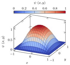
The friction function for a single turbine centred at $(x_{i},y_{i})$ with support radius $r$ and a maximum friction value of $K_{i}$ is thus defined as:

$$C_{i}(\mathbf{m})(x,y)=K_{i}\psi_{x_{i},y_{i},r}(x,y).$$ (3)

Finally, the dimensionless turbine friction function $c_{t}$ in Equation 1 is the sum of the bump functions for all $N$ turbines:

$$c_{t}(\mathbf{m})=\sum_{i=1}^{N}C_{i}(\mathbf{m}).$$ (4)

The functional of interest $J$ describes the value to be maximised and must be differentiable for gradient-based optimisation. Funke et al. [15] chose the time-averaged power extracted from the tidal array due to the increased bottom friction from the presence of turbines. For the steady-state problem considered here the power extraction may be expressed as:

$$J(\mathbf{u},\mathbf{m})=\frac{1}{2}\int_{\Omega}\rho c_{t}(\mathbf{m})\|\mathbf{u}\|^{3},$$ (5)

where $\rho=$1000\text{\,}\mathrm{kg}\text{\,}{\mathrm{m}}^{-3}$$ is the fluid density and $\Omega$ is the domain of interest. For simplicity a cut-in speed and power rating of the turbines is not considered.

2.2 Analytical wake models

From the functional of interest Equation 5 it is clear that power extracted from the tidal flow depends on the positions of the turbines within the array, the flow field, and the applied friction due to the presence of each turbine.

As currents interact with a turbine, energy is extracted, changing the dynamics of the flow. Notably the flow is decelerated behind the turbine and accelerated along its sides. The region around the turbine where flow properties are changed significantly is the wake of the turbine. A simplified model may base a computation of the extracted power of an array on the cube of the flow speed [34, 15] at each of the turbines. Thus the power extracted from the array may be defined as:

$$J(\mathbf{u},\mathbf{m})=\alpha\sum_{i=1}^{N}\lVert\mathbf{u}_{r}(x_{i},y_{i})\rVert^{3},$$ (6)

where $\mathbf{u}_{r}$ is the ‘reduced’ flow field due to the presence of the wakes, and $\alpha$ is a constant incorporating fluid density, the turbine specifications and can potentially also depend on the flow speed.

Simplified models do not include the effects of the turbines on the velocity directly, and thus the dependence of the flow field on the turbine positions must be carefully considered. The wake behind a turbine can be incorporated as an analytical velocity deficit which decreases with increasing distance behind the turbine. Schemes similar to this have been used to optimise turbine layouts within the wind turbine industry [4, 6]. In this case the reduced velocity field can be defined as:

$$\mathbf{u}_{r}(x,y)=c(x,y;\mathbf{m})\mathbf{u}_{a}(x,y),$$ (7)

where $\mathbf{u}_{r}$ and $\mathbf{u}_{a}$ are the reduced and ambient flow fields respectively, whilst $c$ is a combined velocity reduction factor field due to the individual turbine reduction factors resulting from the wakes of the other turbines in the array (discussed in Section 2.3).

It should be noted that analytical wake models of this type differ greatly from a fully coupled model as described in Section 2.1 in that they only affect the local flow field around each turbine and do not impact the flow field upstream of the turbine array, nor in the far-field. In particular, these simplifications preclude the conservation of energy, that is the ambient flow is unaffected by energy extraction by turbines.

2.3 Wind turbine wake models

A number of wake models exist for wind turbines which have been used for optimising arrays of wind turbines. Of note are the Jensen and Larsen models [20, 22]. Whilst these wake models are adequate for small wind arrays [2] they can under-estimate the wake losses in large multi-row arrays [26]. Palm et al. [28] consider such models for the design of tidal turbine arrays; through comparison to CFD simulations, wake models were concluded to hold promise for the appraisal of tidal turbine arrays.

The Jensen model [20] assumes a linearly expanding wake with a velocity deficit that depends only on the distance behind the turbine. The model is defined by the diameter of its wake which depends on the turbine thrust coefficient, a wake decay parameter and the diameter of the turbine. An example wake from the Jensen model is depicted in Figure 4.

The Larsen model [22] derives from Prandtl’s turbulent boundary layer equations. Both first- and second-order approximate solutions to the boundary layer equations exist. It has been demonstrated that in practice there is little difference between the solutions as discrepancies only lie in the near wake field [31] where it would anyway be inefficient to place another turbine. The diameter of the wake in the Larsen model derives from the Prandtl mixing length and the rotor disc area. A flow field around a turbine using the Larsen model is depicted in Figure 4.

Figure 3: The relative $x$ and $y$ coordinates ($x_{0},y_{0}$) of turbine $t_{2}$ in the coordinate system where $t_{1}$ is at the origin and the $x$-axis is aligned with $f$, the flow direction vector at $t_{1}$.

However, both models presented fail to capture the flow fields observed around tidal turbines. As both models are designed for wind turbines they assume a free upper boundary and a fixed lower boundary — the ground. However, in tidal settings the turbine lies between the seabed (a fixed boundary) and the free surface of the water. As there are constraints on the depth in which a turbine may be placed it is likely that the existence of the two bounding surfaces will act to restrict vertical wake expansion. This issue is considered in the context of tidal turbines by Thomson et al. [33] where an eddy-viscosity model [1] is solved locally to each turbine for its downstream velocity deficit using a finite-difference method. The presence of the bounding surfaces is accounted for by limiting vertical wake expansion and extending lateral expansion through the use of an elliptical Gaussian function. This approach is more complex and computationally expensive than the completely analytical wake approaches considered here but may be considered in future research.

A number of other issues exist with the wind wake models. Notably, the parameters controlling the Larsen model are coupled such that it was not possible to produce a wake with similar features to that of the wake behind a marine turbine. Another numerical problem with the Jensen model is that the derivative of the wake reduction factor in the direction perpendicular to the ambient flow is zero. Thus a local gradient-based optimisation algorithm will move turbines apart in the direction of the flow before moving them in the direction perpendicular to the flow. Generally, both the Larsen and Jensen models are problematic for gradient-based optimisation as the wake reduction factor is discontinuous at the edge of the wake (excepting the trailing edge). This has again been observed in numerical experiments where turbines have been badly repositioned by the optimisation algorithm due to a discontinuous gradient.

The core problem with both models is that they do not include zones where the flow is accelerated locally. This feature of the wake is partially responsible for the layouts featuring staggered ‘barrages’ of turbines as demonstrated by Funke et al. [15], thus another wake model must be developed.

2.4 Approximate shallow water wake model

One of the objectives of this work is to produce a simple and efficient model to be used in global optimisation schemes, as a proxy to a shallow water model. A natural choice for such a wake model is one that is produced using the shallow water equations themselves. The reduction factors required by the wake model can be generated by placing a turbine in uniform flow, here $1\text{\,}\mathrm{m}\text{\,}{\mathrm{s}}^{-1}$, and observing the flow field around it. The wake – which predominantly acts in the direction parallel to the free-stream flow with only minor components perpendicular to the free stream flow direction – can be used as a reduction factor ($c$ in Equation 7). For simplicity, only the component parallel to the free stream flow is extracted and taken as a reduction factor. This is shown in Figure 4.

Figure 4: Wake behind a $20\text{\,}\mathrm{m}$ wide turbine placed at the origin in $2\text{\,}\mathrm{m}\text{\,}{\mathrm{s}}^{-1}$ flow using the SWE model (top left), the wake model used in this work (middle left) and their difference (bottom left). Wake behind the same turbine is also modelled using the Jensen and Larsen models (top right and middle right). Each wake was modelled in a domain measuring $1000\text{\,}\mathrm{m}$ by $400\text{\,}\mathrm{m}$, however only the region around the turbine is displayed here

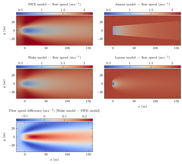
The velocity field of this approximate wake model compared to a shallow water equation simulation with $2\text{\,}\mathrm{m}\text{\,}{\mathrm{s}}^{-1}$ inflow is shown in Figure 5. Visually, the wake appears similar. The difference between the wakes shows that the model is largely accurate with discrepancies lying mostly in the wake directly behind the turbine. Along the centre-line of the wake the approximate wake model overestimates the flow whilst on either side of the centre line it is underestimated. Clear approximations have been made in the selection of the approximate wake model. However, this is deemed sufficient here as this wake model is only used in the first, global stage of the hybrid optimisation approach, and the optimised layout is then fed into the full shallow water model during the second optimisation stage. Future work could improve on this wake model by calculating an ambient flow velocity which is representative of the turbine site of interest before then running a shallow water equation simulation for a single turbine in that flow velocity to generate the wake reduction factor field or by having a ‘library’ of models suitable for different flow speeds.

The product of the individual wake factors is taken to produce the reduction factor

$$c(x,y,\mathbf{m})=\prod_{i=1}^{n}r_{i}(x,y,\mathbf{m}),$$ (8)

where $c$ is the combined factor of $n$ individual reduction factors, $r_{i}$. Whilst a number of combination techniques exist in the literature – such as the sum of squares of velocity deficits employed in the Jensen [20] model – they often do not account for negative velocity deficits, that is where the flow is accelerated. The combination method Equation 8 was chosen for its simplicity and its ability to deal with such cases. Future work could consider an alternative wake combination methods which may be used in cases where the flow velocity increases.

The validity of the combination model was tested by comparing the flow speed behind turbines using the SWE and wake models. A flow of $2\text{\,}\mathrm{m}\text{\,}{\mathrm{s}}^{-1}$ was prescribed with turbines aligned in the direction of flow. For a small number of turbines, the wake combination yields flow velocities adequately close to that produced by the SWE model (Figure 5 depicts this for 3 and 9 turbines). As the number of turbines increases, the difference between the SWE and wake model increases. Specifically, velocities are underestimated in the wake model. During optimisation, should a turbine be in the wake of many others it is likely to be moved out of the wake and thus the errors introduced in this way should be somewhat self-limiting.

Figure 5: Combined wake for the SWE model and the presented wake Equation 7 and combination Equation 8 models. The turbines are spaced $150\text{\,}\mathrm{m}$ and $37.5\text{\,}\mathrm{m}$ apart respectively for the 3 (left) and 9 (right) turbine cases. The inflow of $2\text{\,}\mathrm{m}\text{\,}{\mathrm{s}}^{-1}$ was positioned at $x=0$ in a $50\text{\,}\mathrm{m}$ deep channel. Turbines were aligned parallel to the flow direction with the first turbine positioned at $x=170$ $\mathrm{m}$. The error in combining wakes grows as more wakes are included.

3 Optimisation schemes

Two approaches to global optimisation will be considered in this work: genetic algorithms and a gradient-based ‘basin-hopping’ scheme.

3.1 Genetic algorithms

Genetic algorithms may be described as ‘stochastic search approaches based on randomized operators’ [8] which mimic the process of natural selection. A genetic algorithm operates on a population containing a number of chromosomes, each representing a vector of bits which make up the set of variables used to evaluate the functional of interest in the optimisation problem being posed. Here the chromosome is made up of the positions of the turbines as per Equation 2. The fitness of a chromosome is defined to be the evaluation of the functional of interest, that is the power production of the farm. When applied to optimisation problems the algorithm iteratively applies a number of genetic operators on the population until an exit criteria is met. The typical structure of a genetic algorithm is displayed in Figure 6.

Figure 6: Typical structure of a genetic algorithm. A population of $M$ (here, $100$) chromosomes is initialized, each chromosome representing the location of $N$ turbines. The fitness of each chromosome is evaluated (here the power extracted from the turbine array) so that exit criteria may be checked. If the exit criteria are not met then the selection operator picks $n$ chromosomes (here, $70$ based on a survival rate of $0.7$) from the population and removes the remaining $M-n$ chromosomes. The crossover operator takes the $n$ chosen parents and produces another $M-n$ children which are inserted into the population which is then mutated to introduce new information to the system. The cycle is repeated until the exit criteria are met.

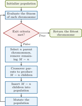
Three main genetic operations are performed during each iteration of the algorithm: selection, crossover and mutation. The role of the selection operator is to pick a number of the fittest chromosomes to propagate through to the next generation (or iteration), the remaining chromosomes are removed from the population. The crossover operator takes the selected chromosomes and produces new ‘children’ chromosomes to replace those not chosen by the selection operator. The mutation operator acts on the new population in order to introduce new information to the system. The new population is evaluated and tested against exit criteria. The cycle is repeated until exit criteria are met. Our genetic algorithm is seeded with a number of sensible automatically generated layouts spanning different areas of the domain as well as randomly generated layouts. The automatically generated layouts include turbines aligned along each edge of the site, along the diagonals, and spread across the site in arrays of varying size and dimension. Further information on genetic algorithms and the operators implemented and used in this work is discussed in general in Haupt and Haupt [19]. Specifics regarding uniform crossover are discussed in more detail in Syswerda [32] and Chawdhry et al. [7] whilst fitness-proportionate mutation is discussed in Pham and Karaboga [29].

3.2 Gradient-based optimisation and ‘basin-hopping’

Genetic algorithms are global in nature and require many iterations to find an optimised state. This is because they depend on randomised operators to search the full solution space. Gradient-based optimisation algorithms are typically local in nature (see Figure 1) and use the gradient of the functional of interest with respect to the parameters to guide the algorithm’s walk through the search space to an optimal solution (Figure 7). This can greatly decrease the number of iterations required for convergence. Consequently this opens up the option for allowing the use of a more costly method to evaluate the functional of interest, i.e. a better approximation of the real world.

Figure 7: Typical gradient-based optimisation algorithm. The functional of interest to be maximised and its gradient are evaluated for input parameters $\mathbf{m}$ to find an ascent direction. The exit criteria are then evaluated. If they are not met then a line search is performed along the ascent direction to find a step size. The parameters are then updated accordingly using the ascent direction and step size. This cycle is repeated until the exit criteria are met.

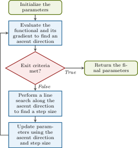
In an attempt to alleviate the limitations of a local optimisation method, Wales and Doye [35] present a stochastic ‘basin-hopping’ algorithm which attempts to find the global maximum of a functional by expanding on a typical gradient-based optimisation algorithm by iteratively performing the following steps (Figure 8):

1. randomly perturb the parameters,

2. perform a local optimisation of the functional (Figure 7),

3. accept or reject the new parameters based on the functional value.

Figure 8: Schematic of the basin-hopping algorithm. After the parameters are initialized they are passed to a local optimization loop (Figure 7). Following local optimization the new parameters are tested against the new parameters (using the Metropolis criterion [24] of standard Monte Carlo algorithms). If the new parameters are accepted they are tested against the exit criteria. If the exit criteria are not met or the parameters were not accepted when tested they are randomly perturbed up to a given step size and passed back to the local optimization algorithm. This process is repeated until the exit criteria are met.

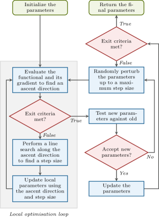
The algorithm employs a variable step size (for the random perturbation) which adjusts according to the rate at which new parameters are accepted or rejected – if the rate at which parameters are accepted is too high then it is likely that the algorithm is stuck in a local maximum, and the step size is increased in order to hop out of the maximum. Due to the more extensive search of the solution space, the basin-hopping algorithm often takes an order of magnitude more iterations than local gradient-based algorithms, and this has to be taken into account in the complexity of the underlying model used.

3.3 Computation and validation of the functional gradient

In this work the gradient of the total power generated by the array with respect to the turbine coordinates is required in order to use gradient-based optimisation. More complex functionals could of course also be used, e.g. those incorporating economic cost models [9]. For the SWE model the generation of the gradient information is achieved via an adjoint calculation using dolfin-adjoint [14, 15]. However, this approach to adjoint development is not applicable to the approximate wake model developed here. Instead, automatic (or algorithmic) differentiation (AD) [18, 27] is used which exploits the fact that no matter how complex an algorithm is, it simply executes a number of simple arithmetic operations and basic functions. AD thus repeatedly applies the chain rule to these procedures to compute derivatives at machine precision. This work employs the ‘ad’ Python package [23] for this purpose.

Unlike a wake model represented as an explicit analytical expression (e.g. as in the Jensen and Larsen models), the standard version of the AD tool cannot be used to calculate certain components of the wake model, such as the spatial derivatives of the wake reduction factor field or ambient flow field as they are stored as FEniCS objects which are not supported by the ad Python package. However, thanks to the FEniCS framework [25] upon which OpenTidalFarm is built it is simple to efficiently and accurately compute these derivatives numerically. The ad package was extended to allow access to the spatial derivatives of the wake reduction factor calculated using DOLFIN (the Python interface to FEniCS).

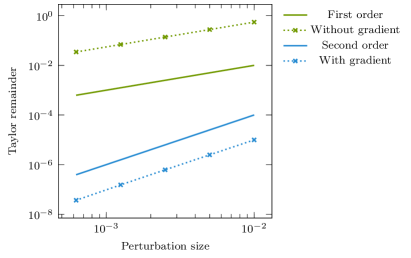
The implementation of the wake model gradient was verified with Taylor remainder convergence tests, similar to Funke et al. [15]. A differentiable functional, $J(\mathbf{m})$ may be expanded about a point $\mathbf{m}+\mathbf{\delta m}$ using Taylor series:

$$J(\mathbf{m})=J(\mathbf{m}+\mathbf{\delta m})-\frac{\mathrm{d}J}{\mathrm{d}\mathbf{m}}\delta\mathbf{m}+\mathcal{O}(\|\delta\mathbf{m}\|^{2}),$$ (9)

thus the convergence order using first-order gradient information should satisfy

$$\left|J(\mathbf{m}+\mathbf{\delta m})-J(\mathbf{m})-\frac{\mathrm{d}J}{\mathrm{d}\mathbf{m}}\delta\mathbf{m}\right|=\mathcal{O}(\|\delta\mathbf{m}\|^{2}).$$ (10)

Equation 10 is a strong test for checking that the gradient computation is correctly implemented. Similarly, we expect the convergence of the functional without gradient information to be of order $\mathcal{O}(\|\delta\mathbf{m}\|^{1})$.

Tests were carried out for a number of flow regimes and parameter sizes ($\delta\mathbf{m}$) to test the validity of the gradient calculation. The results of a test with two turbines deployed randomly in a domain measuring $640\text{\,}\mathrm{m}$ by $320\text{\,}\mathrm{m}$ with a prescribed flow of $(1+x/1280,1+y/640)$ $\mathrm{m}\text{\,}{\mathrm{s}}^{-1}$ (to ensure that the ambient flow has a gradient) are shown in Figure 9. As expected, the model achieves second-order convergence.

Figure 9: Expected (‘First-order’ and ‘Second-order’) and achieved (‘Without gradient’ and ‘With gradient’) orders of convergence in the Taylor remainder tests for the gradient of the wake model. The Taylor remainder is the left hand size of Equation 10 (but only including the first two terms for first-order convergence) whilst the perturbation size is $\mathbf{\delta m}$ in the same equation. Turbine coordinates, $\mathbf{m}$, are perturbed in a random direction by $\mathbf{\delta m}$ from an initial set of chosen coordinates.

4 Results and discussion

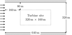
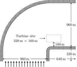
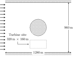
Three test scenarios – scenarios 1, 3 and 4 as per Funke et al. [15] – were used for testing with each turbine site measuring $320\text{\,}\mathrm{m}$ by $160\text{\,}\mathrm{m}$. Schematics of these scenarios are displayed in Figure 10. In the results presented below the following shorthand is used: ‘adjoint’ refers to a gradient-based optimisation, using the SLSQP algorithm [21] for ‘local’ optimisation and the basin-hopping algorithm [35] for ‘global’ optimisation. Both algorithms are available in the SciPy Python package. Optimisation via a genetic algorithm is denoted ‘genetic’. ‘SWE’ refers to the shallow water equations model used by OpenTidalFarm whilst ‘wake’ refers to the approximate wake model developed in this work.

Whilst local and global adjoint optimisation, and genetic optimisation may be used with either the SWE or wake models, it is computationally prohibitive to use global adjoint optimisation and genetic optimisation of the SWE model as discussed in Section 1. Parameters for the model and genetic algorithm (unless otherwise stated) are displayed in Table 1 and Table 2. All experiments were run on a single core of a workstation with an Intel Xeon E3-1240 V2 ($3.4\text{\,}\mathrm{GHz}$) processor and $32\text{\,}\mathrm{G}\mathrm{B}$ of RAM.

(a) Scenario 1: a straight channel.

(b) Scenario 3: a headland.

(c) Scenario 4: a channel between the coast and an island.

Figure 10: Scenarios 1, 3 and 4 as per Funke et al. [15] which were in-turn motivated by Draper et al. [12]. They represent a number of situations which yield fast flow and thus potential tidal array sites. Lines of arrows indicate the inflow (a constant of $2\text{\,}\mathrm{m}\text{\,}{\mathrm{s}}^{-1}$) for the site whilst shaded areas indicate where there is no flow (i.e. land). A dashed box indicates this site the turbines are constrained to reside within.

Parameter	Value
Water depth	$H=$ $50\text{\,}\mathrm{m}$
Viscosity coefficient	$\nu=$ $3\text{\,}{\mathrm{m}}^{2}\text{\,}{\mathrm{s}}^{-1}$
Acceleration due to gravity	$g=$ $9.81\text{\,}\mathrm{m}\text{\,}{\mathrm{}}^{2}\text{\,}{\mathrm{s}}^{-1}$
Water density	$\rho=$ $1000\text{\,}\mathrm{kg}\text{\,}{\mathrm{m}}^{-3}$
Turbine friction coefficient	$K=21$
Bottom friction coefficient	$c_{b}=0.0025$
Turbine radii	$r=$ $10\text{\,}\mathrm{m}$

Table 1: Default parameters used in the experiments unless otherwise stated. Both the turbine friction coefficient and the bottom friction coefficient are dimensionless. The value for the turbine friction coefficient $K$ and the viscosity $\nu$ were motivated by Funke et al. [15].

Option	Value
Selection operator	best $n$ chromosomes
Crossover operator	uniform
Mutation operator	fitness proportionate
Population size	100
Survival rate	0.70
Maximum mutation probability	0.07
Maximum number of iterations	$10000$

Table 2: Parameters used for the genetic algorithm unless otherwise stated. The selection operator takes the best $n=70$ chromosomes as the survival rate of $0.7$ is applied to a population of $100$ chromosomes. These parameters are largely based on trial and error and upon experience.

4.1 Timings

To gain insight into the utility of the wake model, it is beneficial to have an understanding of the relative timings for evaluations of the power extracted from the array as well as the calculation of the gradient of the power with respect to the turbine positions.

The main factor controlling the time to evaluate the power and its gradient in the SWE model is the resolution of the mesh used, whilst the number of turbines and saturation of the site (which is a function of the number of turbines, the size of the turbines and the size of the site) determine the time taken in the wake model. It should be noted that the ambient flow field created for the wake model is generated by the SWE model at a cost which is equivalent to a single power evaluation of the SWE model. Representative timings for the scenarios introduced above as well a more complex Pentland Firth scenario (introduced in Section 5) are presented in Table 3.

Approximate timings for adjoint optimisation can be obtained by taking the product of the number of iterations and the sum of a single power evaluation and a single gradient evaluation. For a genetic optimisation, the approximate time taken is the product of the number of iterations, the population size and the time for a single power evaluation.

Both the power calculation and the gradient of the wake model have an approximate $\mathcal{O}(N^{2})$ complexity as each of the $N$ turbines depends on $N-1$ other turbines. The wake model thus becomes expensive for large numbers of turbines, with gradient evaluations becoming infeasible. Evaluations of the power and gradient in the SWE model utilising the adjoint are largely independent of the number of turbines which remains a significant advantage for this method [15]. The high timings for gradient evaluations of the wake model are due to overhead from the AD tool creating objects for each variable associated with computing the functional of interest. This gradient computation could be made more efficient by tailoring the AD tool to only create objects for the variables relevant to the gradient we are interested in.

Scenario Vertices Power evaluation ($\mathrm{s}$) Gradient evaluation ($\mathrm{s}$) 1 $16556$ $68$ $9$ 3 $31393$ $167$ $19$ 4 $22081$ $126$ $12$ Pentland Firth $50327$ $328$ $32$

(a) Representative timings for the ‘SWE’ model utilising an adjoint calculation in the gradient evaluation. The power evaluation requires a nonlinear SWE solve and thus takes longer to compute than the gradient as the adjoint problem is always linear. Timings are largely independent of the number of turbines $N$ (here, $8$) but depend instead on the resolution of the mesh, that is the number of vertices.

Turbine Site $N$ Power evaluation ($\mathrm{s}$) Gradient evaluation ($\mathrm{s}$) $320\text{\,}\mathrm{m}$ by $160\text{\,}\mathrm{m}$ $8$ $0.03$ $0.6$ $16$ $0.09$ $4$ $32$ $0.3$ $25$ $2000\text{\,}\mathrm{m}$ by $1000\text{\,}\mathrm{m}$ $64$ $0.6$ $20$ $128$ $2$ $155$ $256$ $8$ $1400$

(b) Representative timings for the ‘wake’ model. The $2000\text{\,}\mathrm{m}$ by $1000\text{\,}\mathrm{m}$ site represents the Pentland Firth scenario, whilst the $320\text{\,}\mathrm{m}$ by $160\text{\,}\mathrm{m}$ site is representative of scenarios 1, 3 and 4.

Table 3: Representative timings for evaluations of power and the gradient of power with respect to turbine positions for the SWE model and the wake model. Timings for the ‘SWE’ model are largely dependent on the mesh resolution whilst the size of the turbine site and how saturated it is with turbines heavily influence timings for the wake model. Turbine site saturation is a function of the number of turbines, the size of the turbines and the area of the turbine site. These timings were obtained using turbines measuring $20\text{\,}\mathrm{m}$ by $20\text{\,}\mathrm{m}$ for the $320\text{\,}\mathrm{m}$ by $160\text{\,}\mathrm{m}$ site and $40\text{\,}\mathrm{m}$ by $40\text{\,}\mathrm{m}$ for the $2000\text{\,}\mathrm{m}$ by $1000\text{\,}\mathrm{m}$ site.

4.2 Initial comparison

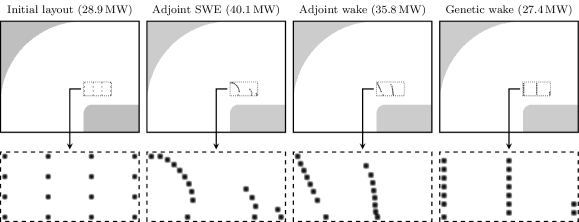
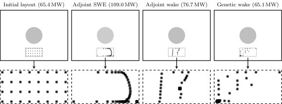
The wake and SWE model were compared in the scenarios presented above for 8, 16 and 32 turbines (a realistic upper limit on the number of turbines that could be deployed in a domain of this size). These initial layouts feature turbines in regular rectangular arrrays ($4\times 2$, $4\times 4$, and $8\times 4$) such that turbines were spaced as far apart as the site allowed. Results are shown in Table 4 with layouts and optimisation convergence plots for three examples shown in Figure 11 and Figure 12.

Table 4 shows that the SWE model consistently produces good results: in all cases the optimised layouts produce significantly more power than the initial layouts at iteration numbers below approximately $100$. The wake model often produces good results using both the adjoint and genetic optimisation approaches: most optimised layouts produce significantly more power than the initial layouts. As expected, the iteration numbers are low with the adjoint based optimisation and higher with the genetic approach.

However, the relative performance of the wake model decreases when the domain becomes saturated with turbines. This is likely due to the simplicity of how the wakes from multiple turbines are combined and highlights a weakness of the wake model to approximate the SWE model when turbines are very close together. This issue results in layouts where a number of turbines overlap. Whilst this may yield a greater power when evaluated by the wake model the same is not necessarily true when evaluated using the shallow water equations. This results in certain optimised layouts being presented as extracting less power than the initial layouts (Table 4, scenario 3 for $1632$ turbines and scenario 4 for $32$ turbines). This is evident in 12(c) where both adjoint and genetic optimisation of the wake model yield layouts with many overlapping turbines. The extracted power in these instances is hypothesised to be locally maximum. In some cases turbines are also observed to overlap in the adjoint optimisation of the SWE model. Providing the optimisation algorithm with a minimum distance constraint for the turbines would provide a solution to this issue but was not done in this work.

Whilst the final power produced using the adjoint wake model is typically lower than that obtained with the SWE model, the time taken is approximately an order of magnitude lower. For example, in scenario 3, optimising 8 turbines with adjoint SWE takes approximately $11500\text{\,}\mathrm{s}$ (over 3 hours) whilst the adjoint optimisation of the wake model takes $520\text{\,}\mathrm{s}$ (under 9 minutes).

It is noted that much of the optimisation via the genetic algorithm is done in the first few iterations and thus the number of iterations before the maximum value is found is often relatively low (Figure 11 and shown in brackets in Table 4). The algorithm does not exit at this point because the rest of the population has not converged on the same solution. Experience indicates that this is due to being seeded with a number of sensible layouts (similar layouts may be achieved without this seeding but in many more iterations). Thus reducing the maximum number of iterations may yield a very similar layout in a fraction of the time.

The results also suggest that in these flat-bottomed domains with relatively simple ambient flow fields the solution space is simple enough to use a local optimisation algorithm, i.e. basin-hopping will offer no advantage.

Scenario	$N$	Optimisation	Iterations	Power ($\mathrm{MW}$)
1	8	Initial	–	$16.08$
		Adjoint SWE	$66$	$48.15$
		Adjoint wake	$102$	$47.04$ ($10.20$)
		Genetic wake	$2315$ ($45$)	$48.35$ ($10.20$)
1	16	Initial	–	$45.81$
		Adjoint SWE	$88$	$69.91$
		Adjoint wake	$91$	$60.92$ ($12.87$)
		Genetic wake	$10000$ ($85$)	$65.14$ ($14.70$)
1	32	Initial	–	$54.49$
		Adjoint SWE	$102$	$95.12$
		Adjoint wake	$141$	$63.26$ ($20.05$)
		Genetic wake	$3009$ ($1045$)	$60.26$ ($19.70$)
3	8	Initial	–	$20.72$
		Adjoint SWE	$63$	$31.33$
		Adjoint wake	$85$	$29.16$ ($11.93$)
		Genetic wake	$5203$ ($1069$)	$25.13$ ($10.55$)
3	16	Initial	–	$28.88$
		Adjoint SWE	$56$	$40.13$
		Adjoint wake	$89$	$35.79$ ($19.07$)
		Genetic wake	$10000$	$27.39$ ($15.08$)
3	32	Initial	–	$30.95$
		Adjoint SWE	$99$	$47.37$
		Adjoint wake	$120$	$34.80$ ($30.33$)
		Genetic wake	$2738$ ($286$)	$26.98$ ($26.69$)
4	8	Initial	–	$30.45$
		Adjoint SWE	$52$	$81.97$
		Adjoint wake	$82$	$70.50$ ($133.37$)
		Genetic wake	$2158$ ($754$)	$53.10$ ($159.84$)
4	16	Initial	–	$65.00$
		Adjoint SWE	$78$	$102.88$
		Adjoint wake	$221$	$82.94$ ($215.39$)
		Genetic wake	$2459$ ($120$)	$73.66$ ($190.78$)
4	32	Initial	–	$65.39$
		Adjoint SWE	$88$	$109.04$
		Adjoint wake	$335$	$76.74$ ($331.18$)
		Genetic wake	$2913$ ($286$)	$65.10$ ($251.41$)

Table 4: Results comparing the number of iterations and power obtained with the SWE and wake model for the three different scenarios considered, each with three numbers of turbines $N$ to be optimised. The initial layouts feature turbines in rectangular arrays with regular spacing making full use of the extent of the turbine site. Some entries for ‘genetic wake’ show two iteration counts; the first represents the total number of iterations while the second bracketed number shows the number of iterations before a power within $2\text{\,}\mathrm{\char 37\relax}$ of the final power was found. The final turbine positions obtained using the wake model were evaluated using the SWE model in order to provide a comparable power estimate in this table. The power as evaluated by the wake model is also shown in brackets. The particularly high power extraction in scenario 4 is due to the cubic dependence of power on flow speed which is close to $4\text{\,}\mathrm{m}\text{\,}{\mathrm{s}}^{-1}$ within the turbine site due to the presence of the ‘island’ in the middle of the domain.

Figure 11: Power extracted from the turbine array using the SWE model optimised using a local gradient-based optimisation algorithm and the wake model using both a local-gradient based optimisation algorithm and a genetic algorithm. The intermediate power was scaled using the SWE model in order to provide a comparable power estimate. The final power achieved by the SWE model is shown as a dotted line for comparison.

(a) Optimised array layouts for 8 turbines in scenario 1. All optimised layouts have similar features; a line of turbines perpendicular to the direction of flow.

(b) Optimised array layouts for 16 turbines in scenario 3. Optimised array layouts have similar features – a longer line of turbines on the left side of the domain. These are angled approximately perpendicular to the direction of the flow for the adjoint SWE and adjoint wake layouts.

(c) Optimised array layouts for 32 turbines in scenario 4. All three layouts contain overlapping turbines, suggesting that the site is too saturated with turbines. The adjoint SWE layout appears to funnel the flow towards the curved wall of turbines, neither of the wake model layouts display this property suggesting that the wake model is too simple for this number of turbines.

Figure 12: Example initial and optimised layouts for three experiments from the initial comparison of the wake model compared to the SWE model. The SWE model was optimised via a local gradient-based optimisation algorithm (adjoint SWE). The wake model was optimised using a local gradient-based optimisation algorithm (adjoint wake) and a genetic algorithm (genetic wake).

4.3 Two stage global-local optimisation

Initial testing indicates that in some situations the wake model with either genetic or adjoint optimisation may be used to get close to the power achieved by the SWE model in a fraction of the time. The optimised layout may be then further optimised using the more accurate SWE model. The aim of this being that a reduction in the number of iterations required of the SWE model would overall result in a more efficient hybrid global-local optimisation approach whilst addressing the problem of local maxima (Figure 1). The same scenarios were tested as per Section 4.2 but the maximum number of iterations for the genetic algorithm was limited to 100 to ensure that the initial global optimisation is cheap (for 32 turbines this time equates to approximately 20 iterations of the SWE model).

Results are presented in Table 5 and show the final optimised power now to be more consistent across optimisation methods. There are no distinct trends amongst the results to suggest a preferred method of optimisation. However, in most cases the number of iterations of the adjoint SWE model in the hybrid approach is lower than that required by just local optimisation of the SWE model. For these cases the total time was reduced on average by approximately $35\text{\,}\mathrm{\char 37\relax}$. This may lead to significant reductions in computation time when considering more realistic scenarios. A number of results from the genetic algorithm optimisation require explanation in light of those obtained in Section 4.2. Scenario 3 with $1632$ turbines and scenario 4 with 32 turbines show higher extracted powers from $100$ iterations than from many thousands of iterations as per Table 4. The results from Table 4 were highlighted above as being due to the simplicity of the wake combination model resulting in overlapping turbines, thus when limited to $100$ iterations the algorithm cannot explore the parameter space so fully, reducing the chance of reaching such a state resulting in a greater power extraction when evaluated by the SWE model.

In some cases the SWE model is seeded with a layout which yields a poor power extraction (see Table 5, scenario 3 with 32 turbines, for example) yet is able to reach a final optimised state which yields a power similar to that achieved by the SWE model alone. This is again indicative that these flat-bottomed domains have a solution space simple enough for a local optimisation algorithm to be used.

Scenario $N$ Optimisation Iterations Power ($\mathrm{MW}$) 1 8 Initial – $16.08$ Adjoint SWE 66 $48.15$ Adjoint wake$\rightarrow$Adjoint SWE 100, 32 $47.04$ ($10.20$)$\rightarrow$$48.67$ Genetic wake$\rightarrow$Adjoint SWE 43, 26 $48.99$ ($9.96$)$\rightarrow$$49.82$ 1 16 Initial – $45.81$ Adjoint SWE 88 $69.91$ Adjoint wake$\rightarrow$Adjoint SWE 89, 55 $60.92$ ($12.87$)$\rightarrow$$62.83$ Genetic wake$\rightarrow$Adjoint SWE 100, 28 $67.48$ ($14.32$)$\rightarrow$$68.23$ 1 32 Initial – $54.49$ Adjoint SWE 102 $95.12$ Adjoint wake$\rightarrow$Adjoint SWE 100, 84 $64.10$ ($19.94$)$\rightarrow$$94.60$ Genetic wake$\rightarrow$Adjoint SWE 7, 35 $78.49$ ($76.47$)$\rightarrow$$79.65$ 3 8 Initial – $20.72$ Adjoint SWE 63 $31.33$ Adjoint wake$\rightarrow$Adjoint SWE 83, 26 $29.16$ ($11.92$)$\rightarrow$$32.34$ Genetic wake$\rightarrow$Adjoint SWE 81, 31 $27.07$ ($46.64$)$\rightarrow$$29.81$ 3 16 Initial – $28.88$ Adjoint SWE 56 $40.13$ Adjoint wake$\rightarrow$Adjoint SWE 87, 48 $35.79$ ($19.07$)$\rightarrow$$44.16$ Genetic wake$\rightarrow$Adjoint SWE 100, 46 $29.81$ ($74.54$)$\rightarrow$$43.77$ 3 32 Initial – $30.95$ Adjoint SWE 99 $47.37$ Adjoint wake$\rightarrow$Adjoint SWE 100, 102 $34.80$ ($30.30$)$\rightarrow$$50.47$ Genetic wake$\rightarrow$Adjoint SWE 100, 135 $32.76$ ($111.07$)$\rightarrow$$50.86$ 4 8 Initial – $30.45$ Adjoint SWE 52 $81.97$ Adjoint wake$\rightarrow$Adjoint SWE 80, 80 $70.50$ ($26.54$)$\rightarrow$$81.88$ Genetic wake$\rightarrow$Adjoint SWE 58, 24 $80.59$ ($145.22$)$\rightarrow$$81.91$ 4 16 Initial – $65.00$ Adjoint SWE 78 $102.88$ Adjoint wake$\rightarrow$Adjoint SWE 100, 57 $82.62$ ($43.13$)$\rightarrow$$102.78$ Genetic wake$\rightarrow$Adjoint SWE 100, 74 $67.31$ ($153.69$)$\rightarrow$$104.30$ 4 32 Initial – $65.39$ Adjoint SWE 88 $109.04$ Adjoint wake$\rightarrow$Adjoint SWE 100, 101 $76.71$ ($64.18$)$\rightarrow$$109.48$ Genetic wake$\rightarrow$Adjoint SWE 100, 97 $73.11$ ($206.38$)$\rightarrow$$107.13$

Table 5: Results comparing two-stage optimisation of the wake model to a single local optimisation of the SWE model. Two-stage optimisation consists of global optimisation of the wake model (adjoint or genetic) followed by local optimisation of the SWE model. This it indicated using the arrow notation ($\rightarrow$).

4.4 Inclusion of bathymetry

The importance of global approaches to optimisation increases with the complexity of the solution space. In tidal turbine array optimisation one important way this occurs is through the addition of non-flat bathymetry. The same optimisation strategies as in Section 4.3 were used. However, in this section the basin-hopping algorithm (which makes use of the local gradient-based approach) was used in the adjoint optimisation of the wake model. The number of iterations allowed by the genetic algorithm was also increased from $100$ to $1000$ to account for the more complex solution space.

Three bathymetry cases were considered. The first bathymetry field is applied to the scenario 1 channel domain from Section 4 and features depth increasing linearly from $25\text{\,}\mathrm{m}30\text{\,}\mathrm{m}$ from the inflow boundary to midway through the domain, at this point the depth decreases rapidly to $25\text{\,}\mathrm{m}$ where it remains constant to the outflow. Thus the fastest current – and hence best location for the turbines – is on the right of the domain, where it is shallowest. However, there is a decrease in flow velocity in the first half of the domain as one moves away from the inflow and thus turbines in this region will not be able to reach the optimal part of the domain using a local algorithm. The bathymetry and ambient flow are displayed in Figure 13.

Figure 13: Bathymetry and flow magnitude due to a $2\text{\,}\mathrm{m}\text{\,}{\mathrm{s}}^{-1}$ flow from the left of the domain for bathymetry 1 and 2. The turbine site is marked by the dotted rectangle.

The second bathymetry, again applied to the scenario 1 domain, contains a randomly generated bathymetry. Unlike bathymetry 1, finding the optimised layout is non-trivial and must be guided by more than intuition. Bathymetry 3 has similar features to bathymetry 2 but is applied to a different domain (scenario 3 as per Section 4). The resulting flow field and bathymetry are presented in Figure 14. The flow speed in the turbine site appears more heavily influenced by the geometry of the domain than the bathymetry, resulting in a simpler solution space than bathymetry 1 and 2.

Figure 14: Bathymetry and flow magnitude due to a $2\text{\,}\mathrm{m}\text{\,}{\mathrm{s}}^{-1}$ flow from the bottom edge of the domain for the whole domain (top) and turbine site (bottom) of bathymetry 3. The turbine site is marked by the dotted rectangle.

Bathymetry $N$ Optimisation Iterations Power ($\mathrm{MW}$) 1 4 Initial – $5.69$ Adjoint SWE $46$ $7.97$ Adjoint wake$\rightarrow$Adjoint SWE $1873$, $45$ $8.87$ ($15.45$)$\rightarrow$$9.12$ Genetic wake$\rightarrow$Adjoint SWE $448$, $23$ $9.09$ ($19.16$)$\rightarrow$$9.18$ 2 4 Initial – $7.05$ Adjoint SWE $7$ $8.56$ Adjoint wake$\rightarrow$Adjoint SWE $1919$, $23$ $10.15$ ($19.36$)$\rightarrow$$10.52$ Genetic wake$\rightarrow$Adjoint SWE $898$, $35$ $10.13$ ($19.94$)$\rightarrow$$10.72$ 3 4 Initial – $6.79$ Adjoint SWE $48$ $9.58$ Adjoint wake$\rightarrow$Adjoint SWE $1915$, $20$ $8.50$ ($24.50$)$\rightarrow$$9.63$ Genetic wake$\rightarrow$Adjoint SWE $614$, $19$ $7.80$ ($22.57$)$\rightarrow$$9.80$

Table 6: Results comparing two-stage optimisation of the wake model to local optimisation of the SWE model for three cases including the effects of bathymetry. Complex bathymetry is likely to cause a number of local maxima, thus global optimisation is essential to finding the optimal layout. Two-stage optimisation consists of global optimisation of the wake model (basin-hopping or genetic) followed by local optimisation of the SWE model. This is indicated using the arrow notation ($\rightarrow$). In bathymetry 2 the initial layout is hypothesised to be very close to a local maximum which is found in seven iterations by the adjoint SWE optimisation. For the two hybrid optimisations of the same bathymetry the number of adjoint SWE iterations is greater as the layout provided by the global optimisation of the wake model is further from a maximum.

Figure 15: Optimisation convergence for bathymetry 1, 2 and 3. The second stage of the optimisation is dotted. A horizontal dashed line representing the final power of the adjoint SWE optimisation is also shown for comparison. The first stages of the adjoint and genetic wake optimisation (shown as solid lines) are scaled such that the final power of the first stage is equal to the first power achieved in the second stage. Thus the power values displayed for the first stage merely show the relative improvement of the optimisation of the wake model and not the actual power extracted. During the first stage of adjoint optimisation in bathymetry 1 after approximately $1000$ iterations the basin-hopping algorithm is unable to escape a local maxima; this is due to the bathymetry of the domain. In this case all turbines are in the right part of the domain where the depth is constant and the turbines are perturbed such that they have little effect on each other. The optimised state occurs near to $600$ iterations where the turbines are in the same part of the domain but are working together to increase the flow speed for the central turbines.

(a) Optimised array layouts for 4 turbines in bathymetry 1.

(b) Optimised array layouts for 4 turbines in bathymetry 2.

Figure 16: Initial and optimised layouts for bathymetry scenarios 1 and 2.

Figure 17: Optimised array layouts for 4 turbines in bathymetry 3.

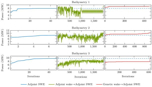
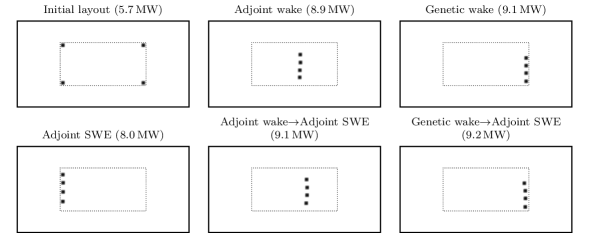
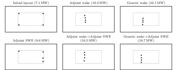
Table 6 displays the results of comparing the SWE model and the wake model in the three different bathymetry scenarios presented above. Convergence plots are presented in Figure 15 whilst initial and optimised layouts are displayed in Figures 16 and 17. Bathymetry 1 and 2 show that using global optimisation schemes (basin-hopping and genetic) can yield significant power improvements over local optimisation schemes whilst a two-stage optimisation yields further improvements. For bathymetry 1, layout optimisation of the SWE model (using the adjoint approach without basin-hopping) results in all turbines on the left hand side of the domain where the flow is slowest whilst both optimisations of the wake model (genetic and using the adjoint approach with basin-hopping) result in turbines on the right hand side of the domain in the faster flowing water (16(a)). After the second stage of optimisation $14.4\text{\,}\mathrm{\char 37\relax}$ and $15.2\text{\,}\mathrm{\char 37\relax}$ improvements are yielded over local optimisation of the SWE model for the adjoint and genetic approaches respectively.

In bathymetry 2 the local optimisation of the SWE model yields a layout somewhat similar to the initial layout (16(b)); we hypothesise that the algorithm is stuck in a local maximum. Both global optimisations of the wake model (genetic and basin-hopping) result in similar layouts. After second stage optimisation the basin-hopping and genetic approaches yield $22.9\text{\,}\mathrm{\char 37\relax}$ and $25.2\text{\,}\mathrm{\char 37\relax}$ improvements over local optimisation of the SWE model.

For bathymetry 3 similar power outputs are achieved for all optimisation approaches. The power achieved by the wake model is $0.5\text{\,}\mathrm{\char 37\relax}$ and $2.3\text{\,}\mathrm{\char 37\relax}$ greater than optimisation of the SWE model for the adjoint and genetic approaches respectively. Importantly, the layouts discovered using the two-stage approach are achieved in approximately $40\text{\,}\mathrm{\char 37\relax}$ less time than those found by the adjoint SWE optimisation (excepting bathymetry 2 where it is hypothesised that the initial layout is very close to a local maximum which is found in very few iterations by the adjoint SWE optimisation).

5 Array optimisation in the Inner Sound of Pentland Firth

The presence of the Orkney Islands accelerates tidal flow through the Pentland Firth separating the Islands from the north east coast of Scotland. This is therefore a site of major interest for tidal turbine array development. The Inner Sound of the Pentland Firth lies in the channel between Stroma Island and Caithness where the water is shallower than the surrounding areas which further accelerates the flow and provides a potential site of appropriate depth for turbine deployment. It is one of the most promising locations for tidal power in the UK and is currently under development by MeyGen Ltd. who have recently been given permission to deploy a first stage of turbines expected to produce $\sim$$86\text{\,}\mathrm{MW}$, with a long term goal of a $\sim$$400\text{\,}\mathrm{MW}$ array.

This site will be used here as a more realistic scenario to demonstrate the work presented above. Layout optimisation of 64 turbines (which is approximately the number required to deliver $86\text{\,}\mathrm{MW}$ of power) will be compared for the local and hybrid global-local approaches as per Section 4.4.

A number of parameters from Table 1 were adjusted to reduce computation time for this larger, more complex problem than was previously considered. The viscosity coefficient, $\nu$ was increased to $100\text{\,}\mathrm{m}\text{\,}{\mathrm{s}}^{-2}$ and the turbine radii to $20\text{\,}\mathrm{m}$. Depth throughout the domain was set using a mixture of the best bathymetry data available in different parts of the domain: from GEBCO [3], Digimap [13] and the Scottish Government [30]. Accurate shoreline data comes from the GSHHS database [36]. The mesh was created using Gmsh [17] and consists of $\sim$$1.0\text{\times}{10}^{5}$ triangles varying from $8.16\text{\,}\mathrm{m}223.14\text{\,}\mathrm{m}$ in size. The domain is the same as used by Funke et al. [15] but includes bathymetry and employs a coarser mesh to reduce computation time. Only the idealised steady flood tide of $2\text{\,}\mathrm{m}\text{\,}{\mathrm{s}}^{-1}$ along the left boundary of the domain is considered in this optimisation.

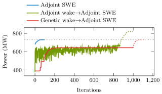
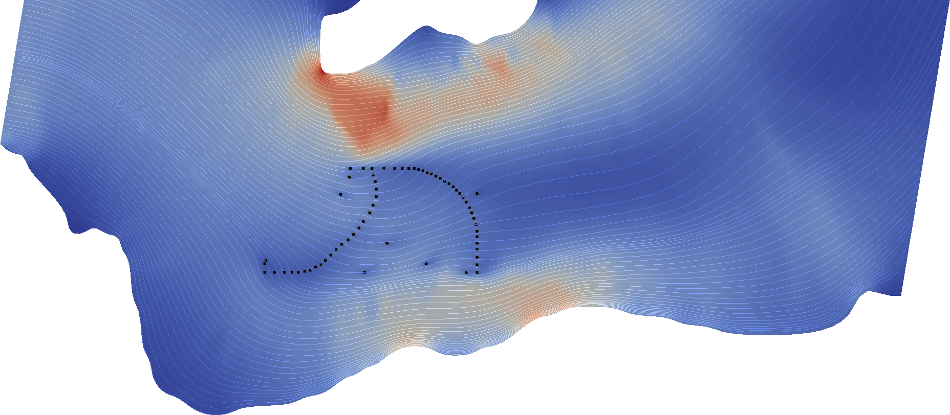
The bathymetry and resulting ambient flow field for the whole domain and the turbine site are displayed in Figure 18, along with the allowed turbine site which is simplified compared to that being considered by MeyGen Ltd. The power extracted from the array configurations is displayed in Table 7 with optimisation convergence displayed in Figure 19. The adjoint two-stage approach yields a 12.2% improvement in power over local optimisation of the SWE model alone, whilst the two-stage genetic approach results in a power similar to local optimisation of the SWE model. It should be emphasised that there are still many simplifications present in the turbine and flow representations and the figures presented need to be viewed in this light.

Figure 18: Bathymetry and flow magnitude for the whole domain (top) and the turbine site (bottom) for the Pentland Firth scenario. The turbine site is shown by the dotted rectangle in the top images.

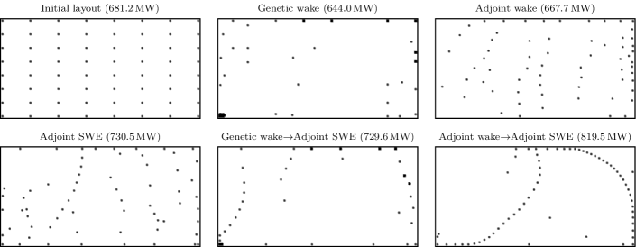
Optimised layouts are displayed in Figure 20. For simplicity, no minimum distance constraints (to enforce a minimum distance between turbines) were used for optimisation. The layout produced by the genetic algorithm features many overlapping turbines which the second stage adjoint SWE optimisation is unable to rectify. The layout which yields the greatest power (‘Adjoint wake$\rightarrow$Adjoint SWE’) features two barrage-like configurations of turbines. A streamline flow visualisation for this layout is presented in Figure 21. Both barrages have similar features; towards the edges the turbines are positioned further upstream than those close to the centre where they are approximately orthogonal to the flow direction. These features help to channel the flow through the array and are conjectured to be the reason for enhanced performance of the design which local optimisation alone was not able to achieve. Funke et al. [15] optimise for 128 and 256 turbines in the same domain but do not include the effects of bathymetry or make use of global optimisation techniques. Whilst this study uses fewer and larger turbines some comparisons may still be hypothesised. Both cases feature barrages of turbines conjectured to guide the flow through the array, however, the inclusion of bathymetry causes the curvature of the barrages to be increased — this is most likely to minimise the number of turbines in the slowest part (south west corner) of the domain whilst still guiding the flow toward the turbines in the faster flowing water in the north eastern part of the turbine site. The large difference in flow velocities in the turbine site is caused by the inclusion of bathymetry; Funke et al. [15] use a constant depth of $50\text{\,}\mathrm{m}$ whilst in this study the bathymetry varies between $5\text{\,}\mathrm{m}$ and $105\text{\,}\mathrm{m}$ with the depth in turbine site varying from $10.6\text{\,}\mathrm{m}35.5\text{\,}\mathrm{m}$. The large difference in depth between the north and south of the domain and throughout the turbine site cause a much broader range of flow magnitudes within the turbine site and is believed to be the reason for the relocation of the barrages.

It is also noted that this layout does not share features with the first optimisation stage (‘Adjoint wake’) which has approximately seven south-south-west to north-north-east trending barrages of turbines (roughly orthogonal to the flow direction). The difference in layouts is most likely due to the simplicity in which the wakes are combined in the wake model. An improved wake combination method is more likely to result in a layout which better matches that achieved after the second optimisation stage. This would also decrease the number of iterations required by the SWE model, significantly reducing computation time. Whilst this relatively low resolution scenario takes approximately $6\text{\,}\mathrm{m}\mathrm{i}\mathrm{n}\mathrm{u}\mathrm{t}\mathrm{e}\mathrm{s}$ for each iteration of the SWE model, the wake model takes approximately $20\text{\,}\mathrm{s}\mathrm{e}\mathrm{c}\mathrm{o}\mathrm{n}\mathrm{d}\mathrm{s}$. This saving would naturally extend to higher resolution problems where computation time may be significantly reduced.

Optimisation	Iterations	Power ($\mathrm{MW}$)
Initial	–	$681.17$
Adjoint SWE	$98$	$730.49$
Adjoint wake$\rightarrow$Adjoint SWE	$864$, $130$	$667.67$$\rightarrow$$819.48$
Genetic wake$\rightarrow$Adjoint SWE	$1000$, $103$	$643.96$$\rightarrow$$729.64$

Table 7: Optimised power from the Pentland Firth scenario. The two stage adjoint optimisation of the wake model yields the highest power yet the power from the layout of the first stage is lower than the initial layout. The case is similar for the two stage genetic optimisation of the wake model but a second stage optimised power is similar to that of local optimisation of the SWE model.

Figure 19: Optimisation convergence for 64 turbines in the Pentland Firth scenario. The second stages of optimisation are shown as dotted lines. The two stage adjoint optimisation (adjoint optimisation of the wake model followed by adjoint optimisation of the SWE model) yields a significant improvement over the adjoint SWE optimisation. The first stages of the adjoint and genetic wake optimisation (solid lines) are scaled such that the final value equals that of the same layout evaluated using the SWE model. Extracted powers for the first stage thus indicate the relative improvement during wake model optimisation and do not necessarily relate to the power which would be extracted from the same layout evaluated by the SWE model.

Figure 20: Initial and optimised layouts for the Pentland Firth scenario. The adjoint wake$\rightarrow$adjoint SWE optimisation represents the optimal array design which contains a number of barrage-like structures to channel the flow through the turbine array. It is noted that the genetic wake layout results in a number of turbines on top of each other. There are a number of reasons which may cause this: inadequacy of the wake model to approximate the SWE model when turbines are in close proximity and the poor suitability of genetic algorithms when optimising for many turbines as the parameter space grows greatly.

Figure 21: Streamline flow visualisation for southern part of the Pentland Firth scenario with the turbine layout acquired using the adjoint wake$\rightarrow$adjoint SWE optimisation for 64 turbines. Turbines toward the edge of each barrage lie further upstream than those in the centre which are approximately aligned orthogonal to the flow.

6 Conclusions

This work presents a wake model which has been demonstrated to act as a proxy to the shallow water model in OpenTidalFarm [15]. The wake model is based upon a reference wake pre-computed using a shallow water equation solver. It provides a relatively cheap computation of the power extracted from a given turbine array layout design and thus allows for global optimisation schemes requiring large numbers of iterations to be used.

The speed of the wake model is its primary strength, however, it suffers in a number of areas. Notably the model is not accurate when the turbine site becomes saturated with turbines. Whether this is actually a problem in realistic industrial applications is yet to be considered (an overly saturated site may not be as viable as a lesser saturated site due to diminishing marginal returns [10]. The inaccuracy of the model is likely to do with the simplistic manner in which wakes from multiple turbines are combined and improvement to this should be considered in future work. Improvements could also be made to the model by generating a reference wake based on a flow speed which is more representative of the site in question and scaling it appropriately.

Experiments utilising the wake model compared genetic and gradient-based algorithms with basin-hopping (i.e. two global optimisers) and show that layouts are generally optimised more effectively using gradient-based approaches. This is particularly true when large numbers of turbines are considered. However, optimisation via genetic algorithms show that seeding the problem with a number of sensible guesses can significantly reduce the number of iterations required for a solution to be found. Future work may extend this idea by considering alternative methods of generating initial turbine layouts as this may significantly decrease the number of iterations required during optimisation.

When optimising layouts in a two-stage approach (global optimisation of the wake model followed by local optimisation of the SWE model), the power extracted from the array is similar to or greater than the power achieved from just locally optimising the array using the SWE model, that is it enables us to mitigate the problem of local maxima. In cases where bathymetry is included, the improvements using two-stage optimisation are shown to be significant with up to $25\text{\,}\mathrm{\char 37\relax}$ improvements for idealised cases and $12\text{\,}\mathrm{\char 37\relax}$ for the more realistic Pentland Firth scenario. Whilst not all cases see a reduction in computation time (due to the wake model producing a poor layout for the second stage of optimisation) many see a reduction in computation time of the order $30\text{\,}\mathrm{\char 37\relax}40\text{\,}\mathrm{\char 37\relax}$. Improvements in the extracted power of this size could be the difference between a turbine array being economically viable or not.

References

- Ainslie [1988] Ainslie, J., 1988. Calculating the flowfield in the wake of wind turbines. Journal of Wind Engineering and Industrial Aerodynamics 27, 213–224. URL: http://dx.doi.org/10.1016/0167-6105(88)90037-2, doi:10.1016/0167-6105(88)90037-2.
- Barthelmie et al. [2007] Barthelmie, R.J., Frandsen, S.T., Nielsen, M.N., Pryor, S.C., Rethore, P.E., Jørgensen, H.E., 2007. Modelling and measurements of power losses and turbulence intensity in wind turbine wakes at Middelgrunden offshore wind farm. Wind Energy 10, 517–528. doi:10.1002/we.238.
- Becker et al. [2009] Becker, J.J., Sandwell, D.T., Smith, W.H.F., Braud, J., Binder, B., Depner, J., Fabre, D., Factor, J., Ingalls, S., Kim, S.H., et al., 2009. Global bathymetry and elevation data at 30 arc seconds resolution: SRTM30_PLUS. Marine Geodesy 32, 355–371. URL: http://dx.doi.org/10.1080/01490410903297766, doi:10.1080/01490410903297766.
- Bilbao and Alba [2009] Bilbao, M., Alba, E., 2009. Simulated Annealing for Optimization of Wind Farm Annual Profit. IEEE. pp. 1–5. URL: http://dx.doi.org/10.1109/LINDI.2009.5258656, doi:10.1109/LINDI.2009.5258656.
- Bryden and Couch [2007] Bryden, I.G., Couch, S.J., 2007. How much energy can be extracted from moving water with a free surface: A question of importance in the field of tidal current energy? Renewable Energy 32, 1961–1966. URL: http://dx.doi.org/10.1016/j.renene.2006.11.006, doi:10.1016/j.renene.2006.11.006.
- Changshui et al. [2011] Changshui, Z., Guangdong, H., Jun, W., 2011. A fast algorithm based on the submodular property for optimization of wind turbine positioning. Renewable Energy 36, 2951–2958. URL: http://dx.doi.org/10.1016/j.renene.2011.03.045, doi:10.1016/j.renene.2011.03.045.
- Chawdhry et al. [1998] Chawdhry, P.K., Roy, R., Pant, R.K. (Eds.), 1998. Soft Computing in Engineering Design and Manufacturing. Springer London. URL: http://dx.doi.org/10.1007/978-1-4471-0427-8, doi:10.1007/978-1-4471-0427-8.
- Chelouah and Siarry [2000] Chelouah, R., Siarry, P., 2000. A continuous genetic algorithm designed for the global optimization of multimodal functions. Journal of Heuristics 6, 191–213.
- Culley et al. [2014a] Culley, D., Funke, S., Kramer, S., Piggott, M., 2014a. Integration of cost modelling within the micro-siting design optimisation of tidal turbine arrays. In preparation.
- Culley et al. [2014b] Culley, D., Funke, S., Kramer, S., Piggott, M., 2014b. A surrogate-assisted optimisation approach for tidal turbine arrays. In preparation.
- Divett et al. [2013] Divett, T., Vennell, R., Stevens, C., 2013. Optimization of multiple turbine arrays in a channel with tidally reversing flow by numerical modelling with adaptive mesh. Philosophical Transactions of the Royal Society A: Mathematical, Physical and Engineering Sciences 371, 20120251–20120251. URL: http://dx.doi.org/10.1098/rsta.2012.0251, doi:10.1098/rsta.2012.0251.
- Draper et al. [2010] Draper, S., Houlsby, G., Oldfield, M., Borthwick, A., 2010. Modelling tidal energy extraction in a depth-averaged coastal domain. IET Renewable Power Generation 4, 545–554. URL: http://dx.doi.org/10.1049/iet-rpg.2009.0196, doi:10.1049/iet-rpg.2009.0196.
- EDINA [2013] EDINA, 2013. SeaZone hydrospatial [ASCII grid geospatial data]. URL: http://edina.ac.uk/digimap.
- Farrell et al. [2013] Farrell, P.E., Ham, D.A., Funke, S.W., Rognes, M.E., 2013. Automated derivation of the adjoint of high-level transient finite element programs. SIAM Journal on Scientific Computing 35, C369–C393. URL: http://dx.doi.org/10.1137/120873558, doi:10.1137/120873558.
- Funke et al. [2014] Funke, S., Farrell, P., Piggott, M., 2014. Tidal turbine array optimisation using the adjoint approach. Renewable Energy 63, 658–673. URL: http://dx.doi.org/10.1016/j.renene.2013.09.031, doi:10.1016/j.renene.2013.09.031.
- Garrett and Cummins [2008] Garrett, C., Cummins, P., 2008. Limits to tidal current power. Renewable Energy 33, 2485–2490. URL: http://dx.doi.org/10.1016/j.renene.2008.02.009, doi:10.1016/j.renene.2008.02.009.
- Geuzaine and Remacle [2009] Geuzaine, C., Remacle, J.F., 2009. Gmsh: A 3-D finite element mesh generator with built-in pre-and post-processing facilities. International Journal for Numerical Methods in Engineering 79, 1309–1331. doi:10.1002/nme.2579.
- Griewank and Walther [2008] Griewank, A., Walther, A., 2008. Evaluating Derivatives: Principles and Techniques of Algorithmic Differentiation. Second, Society for Industrial and Applied Mathematics. URL: http://dx.doi.org/10.1137/1.9780898717761, doi:10.1137/1.9780898717761.
- Haupt and Haupt [2003] Haupt, R.L., Haupt, S.E., 2003. Practical Genetic Algorithms. Wiley Blackwell (John Wiley & Sons). URL: http://dx.doi.org/10.1002/0471671746, doi:10.1002/0471671746.
- Jensen [1983] Jensen, N., 1983. A note on wind generator interaction. Risø-M-2411.
- Kraft [1988] Kraft, D., 1988. A Software Package for Sequential Quadratic Programming. Deutsche Forschungs- und Versuchsanstalt für Luft und Raumfahrt Köln: Forschungsbericht, Wiss. Berichtswesen d. DFVLR.
- Larsen et al. [1996] Larsen, G.C., Højstrup, J., Aagaard Madsen, H., 1996. Wind fields in wakes, in: 1996 European Union wind energy conference, H.S. Stephens & Associates. pp. 764–768.
- Lee [2013] Lee, A.D., 2013. ad: a Python package for first- and second-order automatic differentation. URL: http://pythonhosted.org/ad/.
- Li and Scheraga [1987] Li, Z., Scheraga, H.A., 1987. Monte Carlo-minimization approach to the multiple-minima problem in protein folding. Proceedings of the National Academy of Sciences 84, 6611–6615. URL: http://dx.doi.org/10.1073/pnas.84.19.6611, doi:10.1073/pnas.84.19.6611.
- Logg et al. [2012] Logg, A., Mardal, K.A., Wells, G., 2012. Automated solution of differential equations by the finite element method: The FEniCS book. volume 84. Springer.
- Méchali et al. [2006] Méchali, M., Barthelmie, R., Frandsen, S., Jensen, L., Réthoré, P.E., 2006. Wake effects at Horns Rev and their influence on energy production, in: European wind energy conference and exhibition, p. 10.
- Naumann [2011] Naumann, U., 2011. The Art of Differentiating Computer Programs. Society for Industrial and Applied Mathematics. URL: http://epubs.siam.org/doi/abs/10.1137/1.9781611972078, doi:10.1137/1.9781611972078.
- Palm et al. [2010] Palm, M., Huijsmans, R., Pourquie, M., Sijtstra, A., 2010. Simple wake models for tidal turbines in farm arrangement, in: 29th International Conference on Ocean, Offshore and Arctic Engineering: Volume 3, pp. 577–587. doi:10.1115/OMAE2010-20966.
- Pham and Karaboga [1997] Pham, D.T., Karaboga, D., 1997. Genetic algorithms with variable mutation rates: Application to fuzzy logic controller design. Proceedings of the Institution of Mechanical Engineers, Part I: Journal of Systems and Control Engineering 211, 157–167. URL: http://dx.doi.org/10.1243/0959651971539975, doi:10.1243/0959651971539975.
- Scottish Government [2013] Scottish Government, 2013. Pentland Firth bathymetry. URL: http://www.scotland.gov.uk/Topics/marine/science/MSInteractive/datatype/Bathymetry/data/PentlandFirthBathymetry.
- Sørensen et al. [2008] Sørensen, T., Thøgersen, M.L., Nielsen, P., Jernesvej, N., 2008. Adapting and calibration of existing wake models to meet the conditions inside offshore wind farms. EMD International A/S. Aalborg .
- Syswerda [1989] Syswerda, G., 1989. Uniform crossover in genetic algorithms, in: Proceedings of the 3rd International Conference on Genetic Algorithms, Morgan Kaufmann Publishers Inc., San Francisco, CA, USA. pp. 2–9. URL: http://dl.acm.org/citation.cfm?id=645512.657265.
- Thomson et al. [2011] Thomson, M., Whelan, J., Gill, L., 2011. The development of a tool for the design and optimisation of tidal stream turbine arrays, in: Proceedings of the 9th European Wave and Tidal Energy Conference, Southampton, UK, 2011.
- Vennell [2012] Vennell, R., 2012. The energetics of large tidal turbine arrays. Renewable Energy 48, 210–219. URL: http://dx.doi.org/10.1016/j.renene.2012.04.018, doi:10.1016/j.renene.2012.04.018.
- Wales and Doye [1997] Wales, D.J., Doye, J.P.K., 1997. Global optimization by basin-hopping and the lowest energy structures of Lennard-Jones clusters containing up to 110 atoms. The Journal of Physical Chemistry A 101, 5111–5116. URL: http://dx.doi.org/10.1021/jp970984n, doi:10.1021/jp970984n.
- Wessel and Smith [1996] Wessel, P., Smith, W.H., 1996. A global, self-consistent, hierarchical, high-resolution shoreline database. Journal of Geophysical Research 101, 8741–8743. doi:10.1029/96JB00104.