Magnetocaloric effect in the spin-1/2121/2 chain with competing interactions

T.S. Tavares(2) and G.A.P. Ribeiro(1,2)111pavan@df.ufscar.br
(1) C.N. Yang Institute for Theoretical Physics
(2) Departamento de Física, Universidade Federal de São Carlos
13565-905 São Carlos-SP, Brazil

State University of New York at Stony Brook
(2) Departamento de Física, Universidade Federal de São Carlos
13565-905 São Carlos-SP, Brazil

Stony Brook
(2) Departamento de Física, Universidade Federal de São Carlos
13565-905 São Carlos-SP, Brazil
NY 11794-3840 (2) Departamento de Física, Universidade Federal de São Carlos
13565-905 São Carlos-SP, Brazil
USA (2) Departamento de Física, Universidade Federal de São Carlos
13565-905 São Carlos-SP, Brazil
Abstract

We study the magnetocaloric effect for the integrable antiferromagnetic Heisenberg spin chain with competing interactions. We computed the Grüneisen parameter, which is closely related to the magnetocaloric effect, for the quantum spin chain in the thermodynamical limit. This is obtained by means of the solution of a set of non-linear integral equations, which describes the thermodynamics of the model. We also provide results for the entropy S𝑆S and the isentropes in the (H,T)𝐻𝑇(H,T) plane.

1 Introduction

The magnetocaloric effect refers to any temperature change of magnetic systems induced by an adiabatic variation of the magnetic field. In the last decade, this effect received increasing attention from experimental as well as theoretical viewpoint [1, 2].

Moreover, the magnetocaloric effect has been described by means of exact and numerical tools in various one-dimensional interacting spin systems[3, 4, 5, 6, 7, 8, 9, 10, 11]. Besides its quantitative description, it has been also observed that there is an enhancement of the magnetocaloric effect in the vicinity of quantum critical points[6, 7].

Recently these studies have been extended to the case of spin-1/2121/2 XX chains with three-spin interactions [10] and Ising-Heisenberg four-spin interactions[11]. A natural extension of these results would be the study of integrable spin-1/2121/2 Heisenberg model with additional interaction among spins further apart. This is specially interesting due to the existence of quasi one-dimensional quantum magnets, which can be described by spin-1/2121/2 with next-nearest neighbour interactions[12].

In this paper, we are interested in the exact computation of the magnetocaloric effect for the integrable antiferromagnetic spin-1/2121/2 Heisenberg model with additional interactions among three and four spins. This can be obtained from the related quantity called Grüneisen parameter ΓH=1T(TH)S=1CH(MT)HsubscriptΓ𝐻1𝑇subscript𝑇𝐻𝑆1subscript𝐶𝐻subscript𝑀𝑇𝐻\Gamma_{H}=\frac{1}{T}\left(\frac{\partial T}{\partial H}\right)_{S}=-\frac{1}{C_{H}}\left(\frac{\partial M}{\partial T}\right)_{H}. We also compute the entropy and the isentropes in the (H,T)𝐻𝑇(H,T) plane. These integrable spin chain with competing interactions (three-spin, four-spin and so on) can be constructed by an arbitrary number of staggering parameters [13, 21, 15, 16].

The thermodynamic quantities required to achieve this goal, like entropy, specific heat and magnetization, are determined as a function of temperature and magnetic field. This is obtained by means of the solution of a finite set of NLIE which arises from the QTM approach [17, 18, 19, 22].

This paper is organized as follows. In section 2, we outline the integrable Hamiltonians and the associated integral equations. In section 3, we present our results for the magnetocaloric effect and the isentropes in the (H,T)𝐻𝑇(H,T) plane. Our conclusions are given in section 4.

2 Hamiltonian and integral equations

The integrable spin-1/2121/2 Heisenberg model with interaction among more spins can be constructed within the quantum inverse scattering method by the introduction of certain staggering spectral parameter[13, 21, 15, 16]. We give below the explicit expression for the three and four spin interaction Hamiltonians [22],

3=18(1+θ12)i=12L[(2+θ12)+2σiσi+1+θ12σiσi+2+(1)iθ1σiσi+1×σi+2],subscript3181superscriptsubscript𝜃12superscriptsubscript𝑖12𝐿delimited-[]2superscriptsubscript𝜃122subscript𝜎𝑖subscript𝜎𝑖1superscriptsubscript𝜃12subscript𝜎𝑖subscript𝜎𝑖2superscript1𝑖subscript𝜃1subscript𝜎𝑖subscript𝜎𝑖1subscript𝜎𝑖2{\cal H}_{3}=\frac{1}{8(1+\theta_{1}^{2})}\sum_{i=1}^{2L}[-(2+\theta_{1}^{2})+2\vec{\sigma}_{i}\cdot\vec{\sigma}_{i+1}+\theta_{1}^{2}\vec{\sigma}_{i}\cdot\vec{\sigma}_{i+2}+(-1)^{i}\theta_{1}\vec{\sigma}_{i}\cdot\vec{\sigma}_{i+1}\times\vec{\sigma}_{i+2}], (1)

and

4=12i=13Lc0,i(θ1,θ2)+c1,i(θ1,θ2)σiσi+1+c2,i(θ1,θ2)σiσi+2+c3,i(θ1,θ2)σiσi+1×σi+2+c4,i(θ1,θ2)σiσi+3+c5,i(θ1,θ2)σiσi+1×σi+3+c6,i(θ1,θ2)σiσi+2×σi+3+c7,i(θ1,θ2)σi(σi+1×(σi+2×σi+3)),subscript412superscriptsubscript𝑖13𝐿subscript𝑐0𝑖subscript𝜃1subscript𝜃2subscript𝑐1𝑖subscript𝜃1subscript𝜃2subscript𝜎𝑖subscript𝜎𝑖1subscript𝑐2𝑖subscript𝜃1subscript𝜃2subscript𝜎𝑖subscript𝜎𝑖2subscript𝑐3𝑖subscript𝜃1subscript𝜃2subscript𝜎𝑖subscript𝜎𝑖1subscript𝜎𝑖2subscript𝑐4𝑖subscript𝜃1subscript𝜃2subscript𝜎𝑖subscript𝜎𝑖3subscript𝑐5𝑖subscript𝜃1subscript𝜃2subscript𝜎𝑖subscript𝜎𝑖1subscript𝜎𝑖3subscript𝑐6𝑖subscript𝜃1subscript𝜃2subscript𝜎𝑖subscript𝜎𝑖2subscript𝜎𝑖3subscript𝑐7𝑖subscript𝜃1subscript𝜃2subscript𝜎𝑖subscript𝜎𝑖1subscript𝜎𝑖2subscript𝜎𝑖3{\cal H}_{4}=\frac{1}{2}\sum_{i=1}^{3L}c_{0,i}(\theta_{1},\theta_{2})+c_{1,i}(\theta_{1},\theta_{2})\vec{\sigma}_{i}\cdot\vec{\sigma}_{i+1}+c_{2,i}(\theta_{1},\theta_{2})\vec{\sigma}_{i}\cdot\vec{\sigma}_{i+2}+\\ c_{3,i}(\theta_{1},\theta_{2})\vec{\sigma}_{i}\cdot\vec{\sigma}_{i+1}\times\vec{\sigma}_{i+2}+c_{4,i}(\theta_{1},\theta_{2})\vec{\sigma}_{i}\cdot\vec{\sigma}_{i+3}+c_{5,i}(\theta_{1},\theta_{2})\vec{\sigma}_{i}\cdot\vec{\sigma}_{i+1}\times\vec{\sigma}_{i+3}+\\ c_{6,i}(\theta_{1},\theta_{2})\vec{\sigma}_{i}\cdot\vec{\sigma}_{i+2}\times\vec{\sigma}_{i+3}+c_{7,i}(\theta_{1},\theta_{2})\vec{\sigma}_{i}\cdot(\vec{\sigma}_{i+1}\times(\vec{\sigma}_{i+2}\times\vec{\sigma}_{i+3})), (2)

where θisubscript𝜃𝑖\theta_{i} are free parameters. The coefficients ck,isubscript𝑐𝑘𝑖c_{k,i} have the periodicity property ck,i+3=ck,isubscript𝑐𝑘𝑖3subscript𝑐𝑘𝑖c_{k,i+3}=c_{k,i} and their explicit forms are given in appendix A. These Hamiltonians can be viewed as a two-chain spin model with zigzag interchain interaction [17] and as a three-chain with multiple interchain interactions[22]. Note that θi0subscript𝜃𝑖0\theta_{i}\rightarrow 0 recover the usual Heisenberg spin chain.

The free-energy in the thermodynamic limit for the above spin chains (1) and (2) are given as follows,

f=e01(M1)βj=1M1(KlnBB¯)(θj1),𝑓subscript𝑒01𝑀1𝛽superscriptsubscript𝑗1𝑀1𝐾ln𝐵¯𝐵subscript𝜃𝑗1f=e_{0}-\frac{1}{(M-1)\beta}\sum_{j=1}^{M-1}\left(K*\operatorname{ln}{B\bar{B}}\right)(-\theta_{j-1}), (3)

where the ground state energy is given by

e0=1211+e|k||j=1M1eikθj1(M1)|2dk.subscript𝑒012superscriptsubscript11superscripte𝑘superscriptsuperscriptsubscript𝑗1𝑀1superscriptei𝑘subscript𝜃𝑗1𝑀12differential-d𝑘e_{0}=-\frac{1}{2}\int_{-\infty}^{\infty}\frac{1}{1+{\rm e}^{|k|}}{\Bigg{|}\frac{\sum_{j=1}^{M-1}{\rm e}^{\mathrm{i}k\theta_{j-1}}}{(M-1)}\Bigg{|}}^{2}{\rm d}k.

The auxiliary functions B=b+1,B¯=b¯+1formulae-sequence𝐵𝑏1¯𝐵¯𝑏1B=b+1,\bar{B}=\bar{b}+1 are solutions a set of non-linear integral equations [22],

lnb(x)ln𝑏𝑥\displaystyle\operatorname{ln}{b(x)} =\displaystyle= βd+(x)+(KlnB(x))(x)(KlnB¯(x))(x+i),𝛽subscript𝑑𝑥𝐾ln𝐵𝑥𝑥𝐾ln¯𝐵𝑥𝑥i\displaystyle\beta d_{+}(x)+(K*\operatorname{ln}{B(x)})(x)-(K*\operatorname{ln}{\bar{B}(x)})(x+\mathrm{i}), (4)
lnb¯(x)ln¯𝑏𝑥\displaystyle\operatorname{ln}{\bar{b}(x)} =\displaystyle= βd(x)(KlnB(xi))(x)+(KlnB¯(x))(x),𝛽subscript𝑑𝑥𝐾ln𝐵𝑥i𝑥𝐾ln¯𝐵𝑥𝑥\displaystyle\beta d_{-}(x)-(K*\operatorname{ln}{B(x-\mathrm{i})})(x)+(K*\operatorname{ln}{\bar{B}(x)})(x), (5)

where β=1/T𝛽1𝑇\beta=1/T, d±(x)=1M1j=1M1π2cosh(π(x+θj1))±H2subscript𝑑plus-or-minus𝑥plus-or-minus1𝑀1superscriptsubscript𝑗1𝑀1𝜋2𝜋𝑥subscript𝜃𝑗1𝐻2d_{\pm}(x)=-\frac{1}{M-1}\sum_{j=1}^{M-1}\frac{\pi}{2\cosh(\pi(x+\theta_{j-1}))}\pm\frac{H}{2}, θ0=0subscript𝜃00\theta_{0}=0 and the symbol * denotes the convolution fg(x)=12πf(xy)g(y)𝑑y𝑓𝑔𝑥12𝜋superscriptsubscript𝑓𝑥𝑦𝑔𝑦differential-d𝑦f*g(x)=\frac{1}{2\pi}\int_{-\infty}^{\infty}f(x-y)g(y)dy. The kernel is given by K(x)=e|k|/2+ikx2cosh[k/2]𝑑k𝐾𝑥superscriptsubscriptsuperscript𝑒𝑘2i𝑘𝑥2𝑘2differential-d𝑘K(x)=\int_{-\infty}^{\infty}\frac{e^{-|k|/2+\mathrm{i}kx}}{2\cosh{\left[k/2\right]}}dk.

3 Grüneisen parameter and entropy

In this section we will present the results for the Grüneisen parameter, which is closely related to the magnetocaloric effect. We will also show the results for the entropy and the isentropes in the (H,T)𝐻𝑇(H,T) plane. The results were obtained from the numerical solution of the above non-linear integral equations. Typically, these equation are solved by iteration and it allows for accurate results of the thermodynamical quantities at finite temperatures and magnetic fields.
Refer to caption
Refer to caption
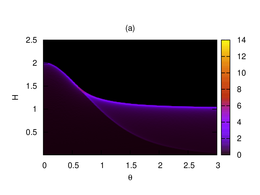
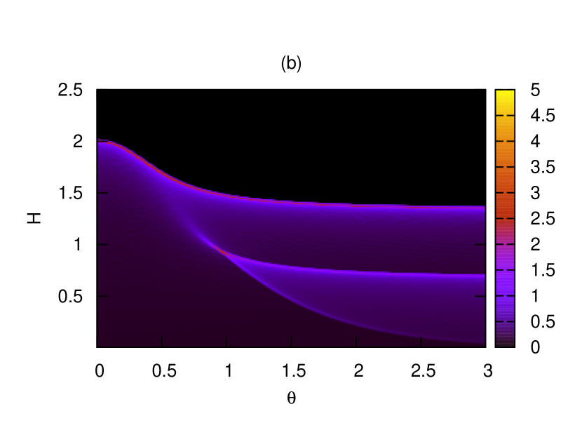
Figure 1: (Color online) Magnetic susceptibility on the plane (H,θ)𝐻𝜃(H,\theta) at T=0𝑇0T=0 for (a) M=3𝑀3M=3 and (b) M=4𝑀4M=4.

In the case of three-spin (M=3𝑀3M=3) interaction Hamiltonian (1), one has three different phases [17, 20, 21, 22]. There is a ferromagnetic phase with gapped excitations where the entropy vanishes and the magnetization saturates and two gapless phases which are the commensurate one for small θ𝜃\theta and the incommensurate one for large θ𝜃\theta [17, 20, 21]. The ground state phase diagram can be read from the magnetic susceptibility at zero temperature, see Figure 1a. In the limits θ=0𝜃0\theta=0 and θ𝜃\theta\rightarrow\infty, we have a single chain of length 2L2𝐿2L and two non-interacting chains of length L𝐿L, respectively.

Refer to captionRefer to caption
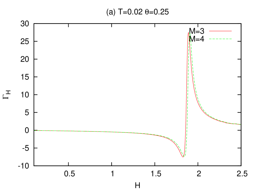
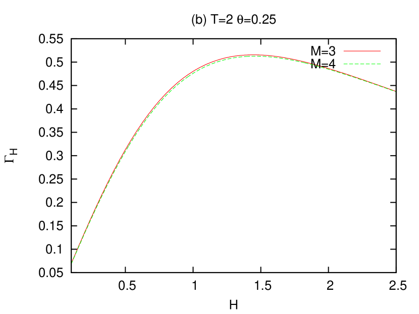
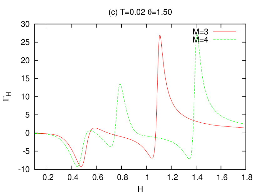
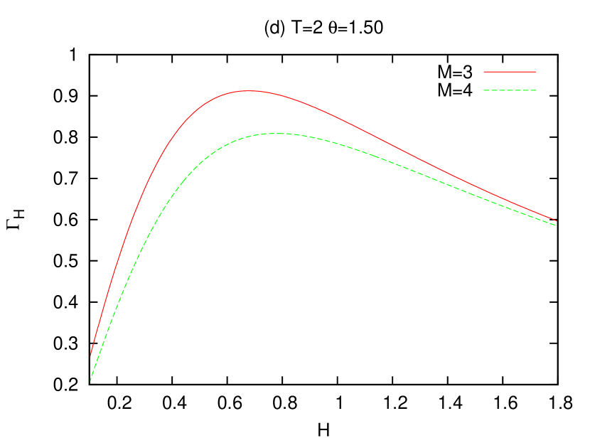
Figure 2: (Color online) The Grüneisen parameter ΓHsubscriptΓ𝐻\Gamma_{H} for M=3,4𝑀34M=3,4 for different values of θ𝜃\theta and temperature: (a) T=0.02𝑇0.02T=0.02 and θ=0.25𝜃0.25\theta=0.25, (b) T=2𝑇2T=2 and θ=0.25𝜃0.25\theta=0.25, (c) T=0.02𝑇0.02T=0.02 and θ=1.5𝜃1.5\theta=1.5 and (d) T=2𝑇2T=2 and θ=1.5𝜃1.5\theta=1.5.

In the Figure 2, for the temperature T=0.02𝑇0.02T=0.02, we can see the transition between the gapless phases and between the gapless and ferromagnetic. This is typically signaled by sign changes of the Grüneisen parameter from negative to positive values toward the higher fields values. For higher temperatures, like T=2𝑇2T=2, we can see that the characteristic behaviour disappears, which implies that the thermal fluctuations are already strong enough to drive the system to excited states where no quantum phase transition effects remain.

On the other hand, in the case of four-spin (M=4𝑀4M=4) interaction Hamiltonian (2), we have chosen θ1=0subscript𝜃10\theta_{1}=0 and θ20subscript𝜃20\theta_{2}\neq 0. This address to the case of two coupled chains of length L𝐿L and 2L2𝐿2L. The chains have different intrachain coupling constants, which result in a superposition of phases [22]. We have four different phases which can be seen in Figure 1b. This can also be noticed at low temperatures by the sign changes in Figure 2a and Figure 2c. In the limits θ0𝜃0\theta\rightarrow 0 and θ𝜃\theta\rightarrow\infty, we have a single chain of length 3L3𝐿3L and two non-interacting chains of different lengths L𝐿L and 2L2𝐿2L, respectively [22].

Refer to caption
Refer to caption
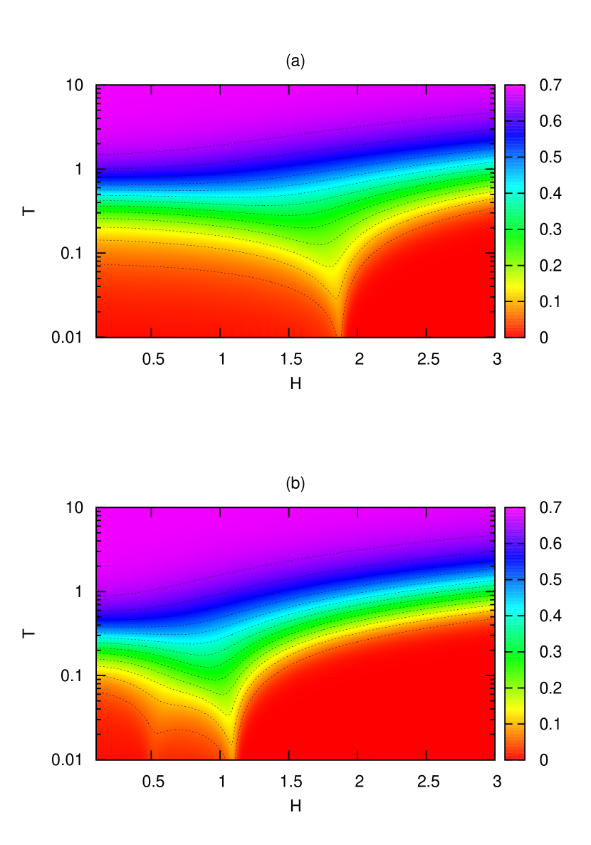
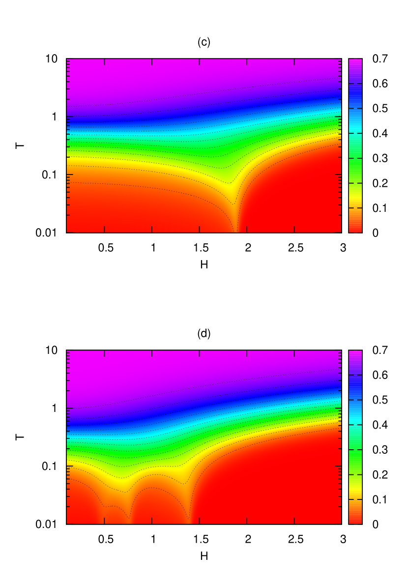
Figure 3: (Color online) Entropy S(H,T)𝑆𝐻𝑇S(H,T) for M=3𝑀3M=3 (a) θ1=0.25subscript𝜃10.25\theta_{1}=0.25 and (b) θ=1.5𝜃1.5\theta=1.5; and for M=4𝑀4M=4 (θ1=0subscript𝜃10\theta_{1}=0) (c) θ2=0.25subscript𝜃20.25\theta_{2}=0.25 and (d) θ2=1.5subscript𝜃21.5\theta_{2}=1.5. The isentropes are for S=0.05,0.1,0.15,,0.65𝑆0.050.10.150.65S=0.05,0.1,0.15,\dots,0.65.

In Figure 3, we present the entropy and the isentropes for the spin chain in the (H,T)𝐻𝑇(H,T) plane for M=3,4𝑀34M=3,4. The quantum phase transitions are indicated by the isentropes, which are tilted towards the quantum critical point[7], showing that the entropy peaks at the critical point[7]. The Grüneisen parameter has a different sign on each side of the quantum critical point as we have shown on Figure 2. This is due to the fact that this parameter is proportional to the slope of the isentropes (TH)Ssubscript𝑇𝐻𝑆\left(\frac{\partial T}{\partial H}\right)_{S}. Moreover, a large magnetocaloric effect is indicated by the steep isentropes nearby the critical point.

4 Conclusion

We studied the magnetocaloric effect in the quantum spin chains with competing interactions involving three and four spins. We exploited the tools of integrability which allow us to construct such integrable chains as well as obtain non-linear integral equations to the thermodynamic quantities. We have computed the Grüneisen parameter in the thermodynamic limit as a function of magnetic field, temperature and the Hamiltonian control θisubscript𝜃𝑖\theta_{i} parameter. In addition, the entropy in the (H,T)𝐻𝑇(H,T) plane and its isentropes have been obtained, which indicates the existence of a large magnetocaloric effect close to the critical points.

Acknowledgments

T.S. Tavares thanks the C.N. Yang Institute for Theoretical Physics for hospitality and FAPESP for financial support through the grant 2013/17338-4. G.A.P. Ribeiro acknowledges financial support through the grant 2012/24514-0, São Paulo Research Foundation (FAPESP).

Appendix A: List of Coefficients 4subscript4{\cal H}_{4}

In this appendix we define explicitly the Hamiltonian coefficients (2).

c0,1subscript𝑐01\displaystyle c_{0,1} =3+2θ22+2(θ2θ1)2+θ22(θ2θ1)26(1+θ22)(1+(θ2θ1)2)absent32superscriptsubscript𝜃222superscriptsubscript𝜃2subscript𝜃12superscriptsubscript𝜃22superscriptsubscript𝜃2subscript𝜃1261superscriptsubscript𝜃221superscriptsubscript𝜃2subscript𝜃12\displaystyle=-\frac{3+2\theta_{2}^{2}+2{(\theta_{2}-\theta_{1})}^{2}+\theta_{2}^{2}{(\theta_{2}-\theta_{1})}^{2}}{6(1+\theta_{2}^{2})(1+{(\theta_{2}-\theta_{1})}^{2})} (A.1)
c0,2subscript𝑐02\displaystyle c_{0,2} =3+2θ12+2(θ2θ1)2+θ12(θ2θ1)26(1+θ12)(1+(θ2θ1)2)absent32superscriptsubscript𝜃122superscriptsubscript𝜃2subscript𝜃12superscriptsubscript𝜃12superscriptsubscript𝜃2subscript𝜃1261superscriptsubscript𝜃121superscriptsubscript𝜃2subscript𝜃12\displaystyle=-\frac{3+2\theta_{1}^{2}+2{(\theta_{2}-\theta_{1})}^{2}+\theta_{1}^{2}{(\theta_{2}-\theta_{1})}^{2}}{6(1+\theta_{1}^{2})(1+{(\theta_{2}-\theta_{1})}^{2})} (A.2)
c0,3subscript𝑐03\displaystyle c_{0,3} =3+2θ12+2θ22+θ12θ226(1+θ12)(1+θ22)absent32superscriptsubscript𝜃122superscriptsubscript𝜃22superscriptsubscript𝜃12superscriptsubscript𝜃2261superscriptsubscript𝜃121superscriptsubscript𝜃22\displaystyle=-\frac{3+2\theta_{1}^{2}+2\theta_{2}^{2}+\theta_{1}^{2}\theta_{2}^{2}}{6(1+\theta_{1}^{2})(1+\theta_{2}^{2})} (A.3)
c1,1subscript𝑐11\displaystyle c_{1,1} =16(1+θ12)(1+θ22)+13(1+(θ2θ1)2)absent161superscriptsubscript𝜃121superscriptsubscript𝜃22131superscriptsubscript𝜃2subscript𝜃12\displaystyle=\frac{1}{6(1+{\theta_{1}}^{2})(1+{\theta_{2}}^{2})}+\frac{1}{3(1+{(\theta_{2}-\theta_{1})}^{2})} (A.4)
c1,2subscript𝑐12\displaystyle c_{1,2} =16(1+θ22)(1+(θ2θ1)2)+13(1+θ12)absent161superscriptsubscript𝜃221superscriptsubscript𝜃2subscript𝜃12131superscriptsubscript𝜃12\displaystyle=\frac{1}{6(1+{\theta_{2}}^{2})(1+{(\theta_{2}-\theta_{1})}^{2})}+\frac{1}{3(1+{\theta_{1}}^{2})} (A.5)
c1,3subscript𝑐13\displaystyle c_{1,3} =16(1+θ12)(1+(θ2θ1)2)+13(1+θ22)absent161superscriptsubscript𝜃121superscriptsubscript𝜃2subscript𝜃12131superscriptsubscript𝜃22\displaystyle=\frac{1}{6(1+{\theta_{1}}^{2})(1+{(\theta_{2}-\theta_{1})}^{2})}+\frac{1}{3(1+{\theta_{2}}^{2})} (A.6)
c2,1subscript𝑐21\displaystyle c_{2,1} =θ126(1+θ12)(1+θ22)+(θ2θ1)26(1+θ22)(1+(θ2θ1)2)absentsuperscriptsubscript𝜃1261superscriptsubscript𝜃121superscriptsubscript𝜃22superscriptsubscript𝜃2subscript𝜃1261superscriptsubscript𝜃221superscriptsubscript𝜃2subscript𝜃12\displaystyle=\frac{\theta_{1}^{2}}{6(1+{\theta_{1}}^{2})(1+{\theta_{2}}^{2})}+\frac{{(\theta_{2}-\theta_{1})}^{2}}{6(1+{\theta_{2}}^{2})(1+{(\theta_{2}-\theta_{1})}^{2})} (A.7)
c2,2subscript𝑐22\displaystyle c_{2,2} =θ126(1+θ12)(1+(θ2θ1)2)+θ226(1+θ22)(1+(θ2θ1)2)absentsuperscriptsubscript𝜃1261superscriptsubscript𝜃121superscriptsubscript𝜃2subscript𝜃12superscriptsubscript𝜃2261superscriptsubscript𝜃221superscriptsubscript𝜃2subscript𝜃12\displaystyle=\frac{\theta_{1}^{2}}{6(1+{\theta_{1}}^{2})(1+{(\theta_{2}-\theta_{1})}^{2})}+\frac{{\theta_{2}}^{2}}{6(1+{\theta_{2}}^{2})(1+{(\theta_{2}-\theta_{1})}^{2})} (A.8)
c2,3subscript𝑐23\displaystyle c_{2,3} =θ226(1+θ12)(1+θ22)+(θ2θ1)26(1+θ12)(1+(θ2θ1)2)absentsuperscriptsubscript𝜃2261superscriptsubscript𝜃121superscriptsubscript𝜃22superscriptsubscript𝜃2subscript𝜃1261superscriptsubscript𝜃121superscriptsubscript𝜃2subscript𝜃12\displaystyle=\frac{\theta_{2}^{2}}{6(1+{\theta_{1}}^{2})(1+{\theta_{2}}^{2})}+\frac{{(\theta_{2}-\theta_{1})}^{2}}{6(1+{\theta_{1}}^{2})(1+{(\theta_{2}-\theta_{1})}^{2})} (A.9)
c3,1subscript𝑐31\displaystyle c_{3,1} =θ16(1+θ12)(1+θ22)+θ1θ26(1+θ22)(1+(θ1θ2)2)absentsubscript𝜃161superscriptsubscript𝜃121superscriptsubscript𝜃22subscript𝜃1subscript𝜃261superscriptsubscript𝜃221superscriptsubscript𝜃1subscript𝜃22\displaystyle=\frac{\theta_{1}}{6(1+{\theta_{1}}^{2})(1+{\theta_{2}}^{2})}+\frac{\theta_{1}-\theta_{2}}{6(1+{\theta_{2}}^{2})(1+{(\theta_{1}-\theta_{2})}^{2})} (A.10)
c3,2subscript𝑐32\displaystyle c_{3,2} =θ16(1+θ12)(1+(θ2θ1)2)+θ26(1+θ22)(1+(θ1θ2)2)absentsubscript𝜃161superscriptsubscript𝜃121superscriptsubscript𝜃2subscript𝜃12subscript𝜃261superscriptsubscript𝜃221superscriptsubscript𝜃1subscript𝜃22\displaystyle=\frac{-\theta_{1}}{6(1+{\theta_{1}}^{2})(1+{(\theta_{2}-\theta_{1})}^{2})}+\frac{-\theta_{2}}{6(1+{\theta_{2}}^{2})(1+{(\theta_{1}-\theta_{2})}^{2})} (A.11)
c3,3subscript𝑐33\displaystyle c_{3,3} =θ26(1+θ12)(1+θ22)+θ2θ16(1+θ12)(1+(θ1θ2)2)absentsubscript𝜃261superscriptsubscript𝜃121superscriptsubscript𝜃22subscript𝜃2subscript𝜃161superscriptsubscript𝜃121superscriptsubscript𝜃1subscript𝜃22\displaystyle=\frac{\theta_{2}}{6(1+{\theta_{1}}^{2})(1+{\theta_{2}}^{2})}+\frac{\theta_{2}-\theta_{1}}{6(1+{\theta_{1}}^{2})(1+{(\theta_{1}-\theta_{2})}^{2})} (A.12)
c4,1subscript𝑐41\displaystyle c_{4,1} =θ22(θ2θ1)26(1+θ22)(1+(θ2θ1)2),absentsuperscriptsubscript𝜃22superscriptsubscript𝜃2subscript𝜃1261superscriptsubscript𝜃221superscriptsubscript𝜃2subscript𝜃12\displaystyle=\frac{{\theta_{2}}^{2}{(\theta_{2}-\theta_{1})}^{2}}{6(1+{\theta_{2}}^{2})(1+{(\theta_{2}-\theta_{1})}^{2})}, c4,2=θ12(θ2θ1)26(1+θ12)(1+(θ2θ1)2)subscript𝑐42superscriptsubscript𝜃12superscriptsubscript𝜃2subscript𝜃1261superscriptsubscript𝜃121superscriptsubscript𝜃2subscript𝜃12\displaystyle c_{4,2}=\frac{{\theta_{1}}^{2}{(\theta_{2}-\theta_{1})}^{2}}{6(1+{\theta_{1}}^{2})(1+{(\theta_{2}-\theta_{1})}^{2})} (A.13)
c4,3subscript𝑐43\displaystyle c_{4,3} =θ12θ226(1+θ12)(1+θ22),absentsuperscriptsubscript𝜃12superscriptsubscript𝜃2261superscriptsubscript𝜃121superscriptsubscript𝜃22\displaystyle=\frac{{\theta_{1}}^{2}{\theta_{2}}^{2}}{6(1+{\theta_{1}}^{2})(1+{\theta_{2}}^{2})}, c5,1=(θ1θ2)θ226(1+θ22)(1+(θ2θ1)2)subscript𝑐51subscript𝜃1subscript𝜃2superscriptsubscript𝜃2261superscriptsubscript𝜃221superscriptsubscript𝜃2subscript𝜃12\displaystyle c_{5,1}=\frac{{(\theta_{1}-\theta_{2})}{\theta_{2}}^{2}}{6(1+{\theta_{2}}^{2})(1+{(\theta_{2}-\theta_{1})}^{2})} (A.14)
c5,2subscript𝑐52\displaystyle c_{5,2} =θ1(θ2θ1)26(1+θ12)(1+(θ2θ1)2),absentsubscript𝜃1superscriptsubscript𝜃2subscript𝜃1261superscriptsubscript𝜃121superscriptsubscript𝜃2subscript𝜃12\displaystyle=\frac{{-\theta_{1}}{(\theta_{2}-\theta_{1})}^{2}}{6(1+{\theta_{1}}^{2})(1+{(\theta_{2}-\theta_{1})}^{2})}, c5,3=θ2θ126(1+θ12)(1+θ22)subscript𝑐53subscript𝜃2superscriptsubscript𝜃1261superscriptsubscript𝜃121superscriptsubscript𝜃22\displaystyle c_{5,3}=\frac{\theta_{2}{\theta_{1}}^{2}}{6(1+{\theta_{1}}^{2})(1+{\theta_{2}}^{2})} (A.15)
c6,1subscript𝑐61\displaystyle c_{6,1} =θ2(θ1θ2)26(1+θ22)(1+(θ2θ1)2),absentsubscript𝜃2superscriptsubscript𝜃1subscript𝜃2261superscriptsubscript𝜃221superscriptsubscript𝜃2subscript𝜃12\displaystyle=\frac{-\theta_{2}{(\theta_{1}-\theta_{2})}^{2}}{6(1+{\theta_{2}}^{2})(1+{(\theta_{2}-\theta_{1})}^{2})}, c6,2=(θ2θ1)θ126(1+θ12)(1+(θ2θ1)2)subscript𝑐62subscript𝜃2subscript𝜃1superscriptsubscript𝜃1261superscriptsubscript𝜃121superscriptsubscript𝜃2subscript𝜃12\displaystyle c_{6,2}=\frac{(\theta_{2}-\theta_{1}){\theta_{1}}^{2}}{6(1+{\theta_{1}}^{2})(1+{(\theta_{2}-\theta_{1})}^{2})} (A.16)
c6,3subscript𝑐63\displaystyle c_{6,3} =θ1θ226(1+θ12)(1+θ22),absentsubscript𝜃1superscriptsubscript𝜃2261superscriptsubscript𝜃121superscriptsubscript𝜃22\displaystyle=\frac{\theta_{1}{\theta_{2}}^{2}}{6(1+{\theta_{1}}^{2})(1+{\theta_{2}}^{2})}, c7,1=θ2(θ1θ2)6(1+θ22)(1+(θ2θ1)2)subscript𝑐71subscript𝜃2subscript𝜃1subscript𝜃261superscriptsubscript𝜃221superscriptsubscript𝜃2subscript𝜃12\displaystyle c_{7,1}=\frac{{-\theta_{2}}(\theta_{1}-\theta_{2})}{6(1+{\theta_{2}}^{2})(1+{(\theta_{2}-\theta_{1})}^{2})} (A.17)
c7,2subscript𝑐72\displaystyle c_{7,2} =θ1(θ2θ1)6(1+θ12)(1+(θ2θ1)2),absentsubscript𝜃1subscript𝜃2subscript𝜃161superscriptsubscript𝜃121superscriptsubscript𝜃2subscript𝜃12\displaystyle=\frac{-\theta_{1}{(\theta_{2}-\theta_{1})}}{6(1+{\theta_{1}}^{2})(1+{(\theta_{2}-\theta_{1})}^{2})}, c7,3=θ1θ26(1+θ12)(1+θ22)subscript𝑐73subscript𝜃1subscript𝜃261superscriptsubscript𝜃121superscriptsubscript𝜃22\displaystyle c_{7,3}=\frac{{\theta_{1}}{\theta_{2}}}{6(1+{\theta_{1}}^{2})(1+{\theta_{2}}^{2})} (A.18)

References

  • [1] A.M. Tishin and Y.I. Spichkin, The magnetocaloric effect and its applications, Institute of Physics Publishing, Bristol (2003).
  • [2] K.A. Gschneidner Jr., V.K. Pecharsky and A.O. Tsokol, Rep. Prog. Phys. 68, 1479 (2005).
  • [3] M.E. Zhitomirsky and A. Honecker, J. Stat. Mech.: Theor. Exp. P07012 (2004).
  • [4] A. Honecker and S. Wessel, Cond. Matt. Phys. 12, 399 (2009).
  • [5] A.S. Boyarchenkov, I.G. Bostrem, A.S. Ovchinnikov, Phys. Rev. B, 76, 224410 (2007).
  • [6] L. Zhu, M. Garst, A. Rosch and Q. Si, Phys. Rev. Lett. 91, 066404 (2003).
  • [7] M. Garst and A. Rosch, Phys. Rev. B, 72, 205129 (2005)
  • [8] C. Trippe, A. Honecker, A. Klümper and V. Ohanyan, Phys. Rev. B 81, 054402 (2010).
  • [9] G.A.P. Ribeiro, J. Stat. Mech. (2010) P12016
  • [10] M. Topilko, T. Krokhmalskii, O. Derzhko, V. Ohanyan, Eur. Phys. J. B 85 (2012) 278.
  • [11] L. Gálisová, Cond. Matt. Phys. 17 (2014) 13001:1-10
  • [12] A.A. Tsirlin, I. Rousochatzakis, D. Kasinathan, O. Janson, R. Nath, F. Weickert, C. Geibel, A.M. Läuchli, H. Rosner, Phys. Rev. B 82 (2010) 144426.
  • [13] V. Yu. Popkov and A.A. Zvyagin, Phys. Lett. A 175 (1993) 295; A.A. Zvyagin, Phys. Rev. B 51 (1995) 12579.
  • [14] A.A. Zvyagin, Phys. Rev. B, 57 (1998) 1035; A.A. Zvyagin, Low. Temp. Phys. 26 (2000) 134.
  • [15] D. Arnaudon, R. Poghossian, A. Sedrakyan and P. Sorba, Nucl. Phys. B 588 (2000) 638.
  • [16] V.V. Mkhitaryan, A.G. Sedrakyan, Nucl. Phys. B 673 (2003) 455.
  • [17] A.A. Zvyagin, J. Phys. A: Math. Gen. 34 (2001) R21.
  • [18] A.A. Zvyagin and A. Klümper, Phys. Rev. B 68 (2003) 144426.
  • [19] C. Trippe and A. Klümper, Low Temp. Phys. 33 (2007) 920.
  • [20] H. Frahm and C. Rödenbeck, J. Phys. A: Math. Gen. 30 (1997) 4467; H. Frahm and C. Rödenbeck, Eur. Phys. J. B, 10 (1999) 409.
  • [21] A.A. Zvyagin, Phys. Rev. B, 57 (1998) 1035; A.A. Zvyagin, Low. Temp. Phys. 26 (2000) 134.
  • [22] T.S. Tavares, G.A.P. Ribeiro, J. Stat. Mech. (2013) P09007.