Drunken robber, tipsy cop: First passage times, mobile traps, and Hopf bifurcations

Abstract

For a random walk on a confined one-dimensional domain, we consider mean first passage times (MFPT) in the presence of a mobile trap. The question we address is whether a mobile trap can improve capture times over a stationary trap. We consider two scenarios: a randomly moving trap and an oscillating trap. In both cases, we find that a stationary trap actually performs better (in terms of reducing expected capture time) than a very slowly moving trap; however, a trap moving sufficiently fast performs better than a stationary trap. We explicitly compute the thresholds that separate the two regimes. In addition, we find a surprising relation between the oscillating trap problem and a moving-sink problem that describes reduced dynamics of a single spike in a certain regime of the Gray-Scott model. Namely, the above-mentioned threshold corresponds precisely to a Hopf bifurcation that induces oscillatory motion in the location of the spike. We use this correspondence to prove the uniqueness of the Hopf bifurcation.

Key words: mean first passage time, mobile trap, Hopf-bifurcation, reaction-diffusion, matched asymptotics, boundary layer

1 Introduction

Numerous problems in nature can be formulated in terms of expected escape time of Brownian particles in the presence of traps. This escape time is often referred to as the mean first passage time (MFPT). For example, a cell is regulated by chemical reactions involving a small number of signaling molecules that have to find their targets in a complex and crowded environment [1]. Further examples include oxygen transport in muscle tissue [2], cold atoms in optical traps [3], molecular self-assembly [4], optimal search strategies [5, 6], and proteins searching for target sequences on a DNA strand [7, 8, 9, 10, 11, 12].

In a recent review of MFPT processes on confined domains [12], it was remarked that while the case of stationary traps is well studied, MFPT problems with mobile traps in confined domains still remain largely unexplored. It is only recently that attention has shifted to mobile traps [13, 14, 15, 16], which is not only more realistic in many situations, but can significantly alter the system’s behaviour. In this paper, we formulate two MFPT problems with a mobile trap on a confined one-dimensional domain and study the effect of trap motion on the average MFPT.

Mobile traps occur naturally in a variety of scenarios. An early example was introduced in [17] for the annihilation reaction $A+B\to 0$, motivated by the annihilation of mobile monopole-antimonopole pairs in the early universe. This general model may also describe chemical kinetics in diffusion-limited regimes [18, 19] where reaction rates are limited by the encounter rate of the reactants, and collision-induced quenching of excited-state particles [20]. Other examples that fit into the mobile traps framework include ligands binding to a receptor on a non-stationary cell, and disease spread [13], where susceptible walkers become infected upon encounter with infected walkers. Perhaps the most common example is that in which predators search for mobile prey [21, 22, 23, 24, 25]. Related MFPT problems with stationary traps involve random walks in the presence of time-constant [26, 27] and time-fluctuating fields [28, 29, 30, 31, 32, 33].

The following scenario illustrates the types of questions that the prototypical MFPT problems below seek to address. Consider a child in a mall that becomes separated from her father. Unable to remember where she initially became separated, the girl performs a random walk in an attempt to locate her father. The question then becomes what the father should do in order to find his daughter in the shortest amount of time. While he might instinctively move about in an active search for the child, it may in fact be more beneficial to remain stationary. The answer depends on the father’s initial location relative to physical boundaries, how fast he moves in relation to the daughter, and what type of motion he follows.

On an infinite domain, it was claimed in [34] for continuous space and proven in [35, 36] for a discrete lattice, that a mobile target in the presence of randomly distributed Brownian traps is always expected to be captured more quickly than a stationary target. In our prototypical examples below, we show that finite domain effects can cause motion to delay expected capture time when the motion is too slow. We note that, unlike [34] and [35], we reverse the role of target and traps so that we compare average capture times in the presence of a stationary versus mobile trap.

We now state the MFPT problems that we analyze below. We consider a particle undergoing a random walk inside an isolated one-dimensional interval, while the trap moves according to the following mechanisms: (A) it undergoes a time-oscillatory motion about the center of the domain with a prescribed frequency and amplitude; and (B) a random walk with prescribed diffusion rate. In each problem, we formulate an associated boundary value problem for the MFPT and compute asymptotic solutions to calculate critical trap speeds below which a mobile trap leads to longer capture times. In a manner analogous to that employed in [13, 24, 37], we show below that the MFPT associated with these two scenarios may be obtained by solving the following two systems:

Problem A: Randomly moving particle with an oscillating trap and reflective endpoints:

$$u_{xx}+u_{t}=-1\,;\qquad u_{x}\left(0,t\right)=0=u_{x}\left(1,t\right)\,,\quad u(x,0)=u(x,2\pi/\omega)\,;$$ (1.1a)

$$u(\xi(t),t)=0\,,\quad\xi(t)=\frac{1}{2}+\varepsilon\sin\left(\omega t\right)\,.$$ (1.1b)

This problem corresponds to a backwards heat equation. Here, $u(x,t)$ denotes the dimensionless mean first passage time (i.e. the expected time to reach the trap) for a particle located at space location $x\in\left(0,1\right)$ at time $t$ within the period of the trap. The trap is assumed to oscillate around the center $x=1/2$ with frequency $\omega$ and amplitude $\varepsilon$, while the endpoints at $x=0,1$ are reflective. For a random walker whose initial location and start time are uniformly distributed over $x\in(0,1)$ and $t\in(0,2\pi/\omega)$, respectively, the expected MFPT is given by

$$\bar{u}=\frac{\omega}{2\pi}\int_{0}^{\frac{2\pi}{\omega}}\int_{0}^{1}\!u(x,t)\,dxdt\,.$$ (1.2)

Surprisingly, this problem is also intimately connected to oscillatory spike motion in certain reaction-diffusion systems such as the Gray-Scott model [38, 39, 40, 41, 42]. This connection will be studied below in Problem C.

Problem B: Randomly moving particle and trap:

$$u_{xx}+a^{2}u_{yy}=-1\,,\qquad\left(x,y\right)\in\left(0,1\right)^{2}\,;$$ (1.3a)

$$\partial_{n}u=0\text{ for }\left(x,y\right)\in\partial\left(\left(0,1\right)^{2}\right)\,,\quad u=0\text{ when }x=y\,.$$ (1.3b)

Here, $u\left(x,y\right)$ is the dimensionless expected time for a particle starting at location $x$ to hit the trap starting at location $y$. The constant $a^{2}$ is the ratio of trap and particle diffusivities. For a randomly moving particle whose starting location is uniformly distributed on $(0,1)$, the expected MFPT is given by

$$\bar{u}(y_{0};{a})=\int_{0}^{1}\!u(x,y_{0})\,dx\,.$$ (1.4)

In (1.4), $y_{0}$ is the initial location of the randomly diffusing trap. The dependence of $\bar{u}$ in (1.4) on $a$ is through that of $u$. We emphasize that the diffusivities of the two random walkers may be different (i.e, $a\neq 1$). For $a=1$, an exact solution of (1.3) may be sought using the method of images. This approach was taken in [43], though instead of solving (1.3) directly, the MFPT was obtained from the solution of the diffusion equation on the same domain with same boundary conditions.

Finally, we show that Problem A is intimately connected to the following problem arising in reaction-diffusion models:

Problem C: A moving sink problem arising from reduced dynamics of an interior spike in the Gray-Scott model:

$$u_{t}=u_{xx}+1-\delta(\xi(t)-x)\,,\qquad u_{x}\left(0,t\right)=0=u_{x}\left(1,t\right)\,;$$ (1.5a)

$$\xi^{\prime}(t)=\beta\left(u_{x}(\xi(t)^{-},t)+u_{x}(\xi(t)^{+},t)\right)\,.$$ (1.5b)

Here, $\xi(t)$ represents the location of the spike as a function of (rescaled) time. In Appendix A, we show how (1.5) is obtained from a certain regime of the Gray-Scott model.

We now summarize our results. For problem A, in the limit of small amplitude $\varepsilon\ll 1$, we calculate a critical frequency $\omega_{c}$ such that a trap with frequency $\omega>\omega_{c}$ performs more optimally (in terms of reducing the average MFPT $\bar{u}$) than a stationary trap. Conversely, for $\omega<\omega_{c}$, trap motion impairs capture time. An algebraic equation for $\omega_{c}$ is given in §2. For problem B, we show that the comparison depends both on the initial location of the trap as well as its speed relative to that of the particle (denoted by $a$). In particular, for a trap initially located at the center of the domain, we find that the moving trap is more optimal when $a>a_{c}\approx 0.53$. In both of these problems, the existence of a critical trap mobility may be inferred by a simple argument. When the trap is stationary ($\omega=a=0$), symmetry dictates that the optimal trap location be at the center of the domain. All other locations are suboptimal. When the trap is barely mobile ($\omega,a\ll 1$), it spends almost all of its time remaining nearly stationary at suboptimal locations. The average MFPT in this case must be larger in comparison to when the trap remains stationary at its optimal location. However, in the limit of high mobility ($\omega,a\gg 1$), the trap may be thought of as everywhere at once, including at the optimal stationary location. In this case, the average MFPT would clearly be smaller in comparison to the stationary trap. There must then exist a “critical mobility” for which the average MFPT’s associated with the stationary and mobile traps are equal.

In problem B, we also investigate how a mobile trap compares to a stationary trap not located optimally at the center of the domain. In the limit of slow trap diffusivity ($a\ll 1$), we find that a stationary trap is more optimal as long as its location $y$ is not “too close” to the boundaries; that is, provided that $y\in\left(y_{c},1-y_{c}\right)$ where $y_{c}=O(a\log a)$. The precise value of $y_{c}$ is given in §3.

By analogy to [21], we refer to problem B as the “drunken robber, drunken cop” problem: both robber and cop are drunk (at different levels of intoxication), and the more they drink, the faster they are assumed to stagger about. Referring to (1.3) where $x$ and $y$ denote the location of the robber and cop, respectively, the case of small $a$ that we study analytically below corresponds to a “drunk robber and tipsy cop”. Roughly speaking, the conclusion is that it is more optimal for the cop to be sober than to be slightly tipsy (as long as he is starting at an “advantageous” location not too close to the boundaries), but it is better still for the cop to be highly inebriated (large $a$) .

Finally, we show the following unexpected relationship between Problems A and C. For small $\beta$ in (1.5), one can show that $\xi\rightarrow 1/2$ at $t\rightarrow\infty$. This equilibrium state becomes unstable due to a Hopf bifurcation as $\beta$ is increased past some $\beta_{hopf}$. At the Hopf bifurcation, we show that the oscillation frequency of $\xi$ is precisely the critical frequency $\omega_{c}$ from Problem A. Furthermore, we exploit this connection to rigorously prove both the existence and uniqueness of $\beta_{hopf}$. This appears to be a general phenomenon; for example, this equivalence (as well as existence and uniqueness) still holds if $u_{xx}$ is replaced by $u_{xx}-\mu u$ in both (1.1) and (1.5).

2 Oscillatory trap

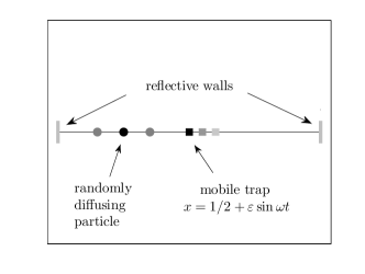
Let us now derive (1.1). Consider a trap that is oscillating around the center of the domain with a given frequency and a small amplitude. We assume insulating boundary conditions. This situation is shown schematically in Figure 1(a). In contrast to cases with stationary traps (see [12] and references therein), the MFPT associated with a location $x$ changes in time due to the motion of the trap. The state of this system may be defined in terms of two variables: the location of the particle, and the location of the trap. Each time step, the particle takes one step either to the left or to the right, while the trap location $\xi(t)$ moves according to the deterministic function $\xi(t)=1/2+\varepsilon\sin(\omega t)$. This suggests that the one-dimensional random walk depicted in Figure 1(a) may be mapped to the equivalent two-dimensional random walk shown in Figure 1(b). Here, the time (vertical) axis assumes the role of the second spatial dimension. The two thick vertical gray lines at $x=0$ and $x=1$ represent the reflective walls, while the $2\pi/\omega$-periodicity in the vertical $t$-axis (horizontal dashed lines) is a consequence of periodic trap dynamics. The mobile trap is mapped to an interior absorbing segment indicated by the solid black curve that divides the domain into a left and right half. Since particles can only stay in one half for their entire lifetime, the mobile trap acts as a spatially dependent absorbing boundary when only the left or right half of the domain is considered (see below).

     

(a) one dimensional random walk with mobile trap

(b) equivalent two-dimensional random walk with drift

Figure 1: (a) A particle undergoing an unbiased random walk with a reflective left and right boundary and a mobile trap oscillating about the center of the domain. (b) The equivalent two-dimensional random walk with deterministic upwards with unit velocity. The thick gray vertical lines at $x=0$ and $x=1$ represent reflective walls. The domain is periodic in $t$, so a particle exiting through the top re-enters at the bottom.

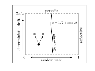
For a two-dimensional walk with random dynamics in the horizontal $x$-direction and deterministic drift in the positive $t$-direction, a static equation for the MFPT $u(x,t)$ associated with location $x$ at time $t$ may be readily derived. In analogy to the derivation of [37] for a discrete random walk with stationary traps, we write

$$u(x,t)=\frac{1}{2}\left[u(x+\Delta x,t+\Delta t)+u(x-\Delta x,t+\Delta t)\right]+\Delta t\,.$$ (2.1)

Equation (2.1) states that the MFPT of a particle located at location $(x,t)$ in the two-dimensional domain is the average of the MFPT associated with the two locations that the particle will next occupy with equal probability, plus the $\Delta t$ time that it takes to move there. Expanding the right-hand side of (2.1) for small $\Delta x$ and $\Delta t$, and defining $D\equiv\Delta x^{2}/(2\Delta t)$, we obtain the following backward-time diffusion equation,

$$Du_{xx}+u_{t}=-1\,,\qquad u_{x}\left(0,t\right)=0=u_{x}(1,t)\,,\quad u(x,0)=u(x,2\pi/\omega)\,;$$ (2.2a)

$$u(\xi\left(t\right),t)=0\,,\quad\xi(t)=\frac{1}{2}+\varepsilon\sin\left(\omega t\right)\,.$$ (2.2b)

The constant $D$ in (2.2a) can be scaled to unity without loss of generality, which leads to the boundary value problem in (1.1). We remark that (2.1) is in contrast to a regular diffusive process, for which the state at $(x,t)$ is an average of states at an earlier time $t-\Delta t$. This is due to the fact that particles captured by the interior absorbing segment in Figure 1(b) have left the system and thus cannot pass information in the direction of drift; instead, information from the absorbing segment propagates in the direction opposite the drift.

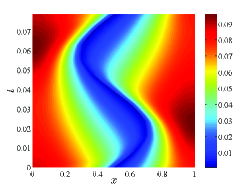
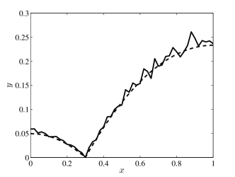
The solution of (1.1) may be computed numerically by solving the associated forward-time diffusion equation (obtained by time-reversing $t\rightarrow-t$ in (1.1)), which quickly converges to a $2\pi/\omega$ time-periodic solution. Alternatively, one can also solve the boundary value problem associated with the $t$-periodic boundary conditions in (1.1). We adopt the latter approach below, using FlexPDE software to solve the associated boundary-value problem. In Figures 2(a) and 2(b), we compare the MFPT as given by the PDE solution of (1.1) with $\varepsilon=0.2$ and $\omega=80$ versus that given by Monte Carlo simulations. The figures depict the MFPT associated with each location in space, at a given instant during the cycle of the trap dynamics. While the trap is located near $x=0.5$ in both figures, the MFPT differs greatly due to the direction of motion of the trap. In particular, the MFPT is high directly behind the trap, and low directly in front of it. Figure 2(c) shows the corresponding space-time plot.

The Monte Carlo results were generated as follows. At a given time $t_{m}\in[0,T)$ during the cycle of trap, 10000 particles are placed at a particular point in space $x_{n}$. Each particle undergoes a random walk and the time to capture is recorded for each. The average of the capture times is then recorded as the MFPT associated with location $x_{n}$ at time $t_{m}$ in the trap’s cycle. Repeating over each location of the discretized domain, we generate a figure of the type in Figures 2(a) and 2(b). The procedure is then repeated for multiple values of $t_{m}$ to capture the time-dependence.

     

(a) trap moving leftward

(b) trap moving rightward

(c) surface plot of MFPT

Figure 2: Comparison of MFPT as given by the PDE solution of (1.1) with $\varepsilon=0.2$ and $\omega=80$ (dashed) versus that given by Monte Carlo simulations (solid). (a) MFPT when the trap is located near $x=0.5$ and moving leftward. (b) MFPT when the trap is located near $x=0.5$ and moving rightward. Note that the MFPT is high (low) directly behind (in front of) the trap. (c) Space-time representation of MFPT from a numerical solution of (1.1).

2.1 Critical oscillation frequency

As stated in the introduction, our goal is to determine the threshold frequency $\omega_{c}$ for which a trap oscillating about $x=1/2$ with amplitude $\varepsilon\ll 1$ and frequency $\omega>\omega_{c}$ performs more optimally than a stationary trap located at $x=1/2$. To facilitate analysis, we exploit the left-right symmetry (see Figure 2(c)) and consider only the left half of the domain $0<x<1/2+\varepsilon\sin\omega t$, $0<t<2\pi/\omega$. On this half-domain, the interior absorbing segment in Figure 1(b) acts as an absorbing Dirichlet boundary. The expression $\bar{u}$ in (1.2) for the average MFPT then becomes

$$\bar{u}=\frac{\omega}{\pi}\int_{0}^{\frac{2\pi}{\omega}}\int_{0}^{1/2+\varepsilon\sin(\omega t)}\!u(x,t)\,dxdt\,.$$ (2.3)

To find $\omega_{c}$ in the limit of small $\varepsilon$, we treat (1.1) as a perturbed boundary problem and compute a three-term regular asymptotic expansion for $u$. That is, we expand $u(x,t)$ as

$$u(x,t)=u_{0}(x)+\varepsilon u_{1}(x,t)+\varepsilon^{2}u_{2}(x,t)\,.$$ (2.4)

In (2.4),

$$u_{0}(x)=-x^{2}/2+1/8$$ (2.5)

is the time-independent MFPT associated with a stationary trap with spatially averaged MFPT $\bar{u}_{0}=1/12$. With (2.4), $\bar{u}$ in (2.3) has the small-$\varepsilon$ expansion,

$$\bar{u}\sim\frac{1}{12}+\varepsilon\frac{\omega}{\pi}\int_{0}^{\frac{2\pi}{\omega}}\int_{0}^{1/2}\!u_{1}(x,t)\,dxdt+\varepsilon^{2}\frac{\omega}{\pi}\left[\int_{0}^{\frac{2\pi}{\omega}}\int_{0}^{1/2}\!u_{2}(x,t)\,dxdt+\int_{0}^{\frac{2\pi}{\omega}}\!u_{1}(1/2,t)\sin\omega t\,dt-\frac{1}{8}\right]\,.$$ (2.6)

We show below that the $\mathcal{O}(\varepsilon)$ term in (2.6) evaluates to zero. The condition on the leading order threshold value of $\omega_{c}$ must then occur when the $\mathcal{O}(\varepsilon^{2})$ term is also zero.

To obtain this condition, we must calculate $u_{1}$ and $u_{2}$ in (2.6). The insulating condition at $x=0$ and the periodicity condition in $t$ remain unchanged for $u_{i}$, $i=0,1,2$. For the Dirichlet condition at $x=\xi(t)$ in (1.1b), we expand for small $\varepsilon$ and collect powers to obtain the following boundary value problems:

$$u_{0xx}+1=0\,;\qquad u_{0x}(0)=0\,,\quad u_{0}(1/2)=0\,;$$ (2.7a)

$$u_{1xx}+u_{1t}=0\,;\qquad u_{1x}(0,t)=0\,,\quad u_{1}(1/2,t)=-\sin\left(\omega t\right)u_{0x}(1/2)\,,\quad u_{1}(x,0)=u_{1}(x,2\pi/\omega)\,;$$ (2.7b)

$$u_{2xx}+u_{2t}=0\,;\qquad u_{2x}(0,t)=0\,,u_{2}(1/2,t)=-\sin(\omega t)u_{1x}-\\ u_{0xx}(1/2)\sin^{2}(\omega t)/2\,,\quad u_{2}(x,0)=u_{2}(x,2\pi/\omega)\,.$$ (2.7c)

The solution for (2.7a) is given by (2.5), while solving for $u_{1}$ in (2.7b) yields

$$u_{1}=e^{it\omega}\frac{\cosh\left(\sqrt{-i\omega}\,x\right)}{4i\cosh(\sqrt{-i\omega}/2)}-e^{-it\omega}\frac{\cosh\left(\sqrt{i\omega}\,x\right)}{4i\cosh(\sqrt{i\omega}/2)}\,.$$ (2.8)

Next, (2.8) with (2.7c) suggests that $u_{2}$ in (2.7c) has the form

$$u_{2}(x,t)=\frac{1}{4}-\frac{1}{8}\sqrt{i\omega}\tanh\left(\sqrt{i\omega}/2\right)-\frac{1}{8}\sqrt{-i\omega}\tanh\left(\sqrt{-i\omega}/2\right)+p(x)\,e^{i2\omega t}+q(x)\,e^{-i2\omega t}\,.$$ (2.9)

Since the $t$-integral in (2.6) of the oscillatory modes in (2.9) evaluate to zero, we find that

$$\bar{u}=\frac{1}{12}+\frac{\varepsilon^{2}}{8}h(\omega)\,,$$ (2.10a)

where

$$h(\omega)\equiv 4-\sqrt{i\omega}\tanh\left(\sqrt{i\omega}/2\right)-\sqrt{-i\omega}\tanh\left(\sqrt{-i\omega}/2\right)\,.$$ (2.10b)

We show below that $h(\omega)$ in (2.10b) is monotonic decreasing and has a unique zero. We therefore conclude that the average MFPT is lower when the trap remains stationary ($\varepsilon=0$) than when it oscillates with small amplitude ($0<\varepsilon\ll 1$) when $0<\omega<\omega_{c}$, where $\omega_{c}\approx 9.6017$ satisfies

$$h(\omega_{c})=0\,.$$ (2.11)

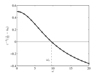
Conversely, the average MFPT is lower in the presence of an oscillating trap when $\omega>\omega_{c}$. In Figure 3(a), we show a favorable comparison between numerically computed values of the quantity $\varepsilon^{-2}(\bar{u}-1/12)$ (circles) and the asymptotic result given by (2.10) (solid curve). The numerical results were obtained from the FlexPDE finite element solver. We note that both plots cross the horizontal axis near $\omega\approx\omega_{c}$.

         

(a) $\varepsilon^{-2}(\bar{u}-\bar{u}_{0})$ versus $\omega$

(b) $\omega_{c}$ versus $\varepsilon$

Figure 3: (a) Comparison between numerically computed values of the quantity $\varepsilon^{-2}(\bar{u}-\bar{u}_{0})$ (circles) and the asymptotic result given by (2.10) (solid curve). Here, $\varepsilon=0.01$. Note the axis crossing near $\omega\approx\omega_{c}$. (b) Critical oscillation frequency $\omega_{c}$ for a range of oscillation amplitude $\varepsilon$. Observe that for $\varepsilon$ small, $\omega_{c}\sim 9.6017$.

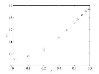
To show that the positive root to $h(\omega)$ exists and is unique, we find an alternative solution to (1.1) using the Fourier series in space (instead of separation of variables in time). After some algebra, we obtain

$$h(\omega)=8\left\{\frac{1}{2}-\sum_{k=0}^{\infty}\frac{1}{\left(2k+1\right)^{4}/\omega^{2}+1}\right\}\,.$$ (2.12)

The equivalence of (2.12) and (2.10) can also be seen directly by using the identity

$$\tanh(s)=\sum_{k=0}^{\infty}\frac{2s}{s^{2}+(\frac{2k+1}{2})^{2}}\,.$$ (2.13)

From (2.12), we observe that $h(\omega)$ is monotonic decreasing since each individual term in the sum is monotonic increasing in $\omega$. Next, we calculate the large $\omega$ asymptotics of the sum in (2.12) as

$$\sum_{k=0}^{\infty}\frac{1}{\left(2k+1\right)^{4}/\omega^{2}+1}\sim\frac{\sqrt{\omega}}{2}\int_{0}^{\infty}\!\frac{1}{1+s^{4}}\,ds\sim\frac{\pi}{4}\sqrt{2\omega}\,,\quad\omega\gg 1\,.$$ (2.14)

With (2.12), (2.14) shows that $h(\omega)\to-\infty$ as $\omega\to\infty$. With $h(0)=4>0$, we thus conclude that $h(\omega)$ is a decreasing function of $\omega$, positive for small $\omega$ and negative for sufficiently large $\omega$. This proves the existence and uniqueness of a positive root of $h(\omega)$.

In §4, we show that the critical frequency $\omega_{c}$ is identical to a Hopf bifurcation frequency of certain regime of the Gray-Scott model, the resulting reduced system of which is given in (1.5). The problem of splitting probability is considered briefly in the discussion section. We show that, in contrast to the MFPT problem, the splitting probability does not exhibit the type of behavior characterized by the existence of a critical oscillation frequency.

3 Brownian trap

In this section, we consider the case of a Brownian trap. To derive a boundary value problem describing the MFPT, we adopt the same approach as in [13, 24]. At each instant in time the system may be defined by the locations $x$ and $y$ of the particle and trap, respectively. Assuming that each undergoes an unbiased discrete random walk, the system in state $(x,y)$ may move to one of its nearest neighbors every $\Delta t$ time step. The two-agent random walk in one dimension can then be mapped onto a one-agent random walk in two dimensions on a rectangular lattice with horizontal and vertical spacings $\Delta x$ and $\Delta y$. The PDE for the MFPT $v(x,y)$ may then be readily obtained in the same manner as in §2. We write

$$v(x,y)=\frac{1}{4}\left(v(x+\Delta x,y)+v(x-\Delta x,y)+v(x,y+\Delta y)+v(x,y-\Delta y)\right)+\Delta t\,,$$ (3.1)

which states that the MFPT associated with the state $(x,y)$ is the average of that of the four states it may evolve to next, plus the $\Delta t$ time that elapses between the transition. Expanding (3.1) for small $\Delta x$ and $\Delta y$ we obtain

$$\frac{\left(\Delta x\right)^{2}}{2\Delta t}v_{xx}+\frac{\left(\Delta y\right)^{2}}{2\Delta t}v_{yy}+1=0\,.$$ (3.2)

Rescaling $v$ in (3.2) by $v=2\Delta t/\left(\Delta x\right)^{2}u$ we then obtain the boundary value (1.3) with $a=\Delta y/\Delta x$.

In Figure 4, we compare the numerical solution of (1.3) with ${a^{2}}=0.1$ against MFPT results from Monte Carlo simulations. In the Monte Carlo simulations, the MFPT associated with a given point $x$ was computed by averaging over $500$ realizations of a randomly diffusing particle-trap pair starting from respective locations $x$ and $y_{0}$. In Figure 4, $y_{0}=0.3$. The capture time of a particular realization was taken to be the time elapsed before the particle and trap locations first coincided.

Figure 4: Comparison of the numerical solution of (1.3) with ${a^{2}}=0.1$ (dashed) against MFPT results from Monte Carlo simulations (solid). The starting location of the trap is $y_{0}=0.3$.

The main question that we seek to address is: For a given speed ratio $a$ and an initial trap location $y_{0}$, is it more optimal for a trap to move randomly or to remain stationary? As in §2, we address this question by comparing the average MFPT over $x$. That is, for a given $a$ and $y_{0}$, we compare $\bar{u}(y_{0};a)=\int_{0}^{1}\!u(x,y_{0})\,dx$ for zero and nonzero $a$. Using the underlying symmetry $u(x,y)=u(1-y,1-x)$ to reduce the domain from a square to a triangle $0<x<y,\ 0<y<1$, this average may then be calculated as

$$\bar{u}(y_{0};{a})=\int_{y_{0}}^{1}\!u(x,y_{0})\,dx+\int_{1-y_{0}}^{1}\!u(x,1-y_{0})\,dx\,.$$ (3.3)

By computing $\bar{u}$ numerically, we find that there is a critical value $a_{c}\approx 0.53$ such that $\bar{u}\left(1/2,a_{c}\right)=\bar{u}\left(1/2,0\right)$ and moreover that $\bar{u}\left(y_{0},a\right)<\bar{u}\left(y_{0},0\right)$ for any $y_{0}$, as long as $a>a_{c}$. That is, regardless of initial trap location, a mobile trap is more optimal (in the sense of reducing $\bar{u}(y_{0};a)$) than a stationary trap as long as the trap moves quickly enough. When $a<a_{c}$, there exists $y_{c}(a)$ such that $\bar{u}(y_{0};a)>\bar{u}(y_{0};0)$ as long as $y_{0}\in\left(y_{c},1-y_{c}\right)$. Moreover, we find analytically that $y_{c}(a)\rightarrow 0$ as $a\rightarrow 0$. We thus conclude that a very slow trap performs worse than a stationary trap except when when its initial location is very close to the boundary. In this limit of a very slow trap, we determine the asymptotic formula for $y_{c}$

$$y_{c}\sim\frac{2}{\pi}a\log\left[\frac{48}{\pi^{3}a}\right]\,,\qquad a\ll 1\,.$$ (3.4)

These results are summarized in Figure 5(a).

The derivation of (3.4) requires the analysis of the contribution of the boundary layer of (1.3) near $y=\mathcal{O}(a)$. In the outer region $y\gg\mathcal{O}(a)$, we write $u\sim u^{o}$ with $u^{o}\sim u_{0}+{a^{2}}u_{1}+O(a^{4})$. From (1.3), both $u_{0}$ and $u_{1}$ satisfy the boundary value problem

$$u_{xx}+1=0\,,\qquad 0<y<1\,,\quad y<x<1\,,\quad u_{x}(1,y)=0\,,\quad u(y,y)=0\,.$$ (3.5)

Solving (3.5), we obtain for the outer solution

$$u^{o}\sim(1+a^{2})\left[\frac{y^{2}}{2}-\frac{x^{2}}{2}+x-y\right]\,.$$ (3.6)

We note that (3.6) does not satisfy the no-flux boundary condition in (1.3b) on the line $y=0$, which will be satisfied by the boundary layer. In this inner region where $y=\mathcal{O}(a)$, we let $u\sim U$ where we expand $U$ as

$$U(x,\eta)=U_{0}+aU_{1}+a^{2}U_{2}\ldots\,;\qquad y=a\eta\,.$$ (3.7)

Next, expanding the Dirichlet boundary condition $U(a\eta,\eta)=0$ along the diagonal $x=y$, we obtain the following boundary value problems,

$$U_{0xx}+U_{0\eta\eta}+1=0\,;\qquad U_{0}(0,\eta)=0\,,\quad U_{0x}(1,\eta)=0,\quad U_{0\eta}(x,0)=0\,;$$ (3.8a)

$$U_{1xx}+U_{1\eta\eta}=0\,;\qquad U_{1}(0,\eta)=-\eta U_{0x}(0,\eta)\,,\quad U_{1x}(1,\eta)=0,\quad U_{1\eta}(x,0)=0\,;$$ (3.8b)

$$U_{2xx}+U_{2\eta\eta}=0\,;\qquad U_{2}(0,\eta)=-\frac{\eta^{2}}{2}U_{0xx}(0,\eta)-\eta U_{1x}(0,\eta)\,,\\ \quad U_{2x}(1,\eta)=0,\quad U_{2\eta}(x,0)=0\,.$$ (3.8c)

To determine the large-$\eta$ behaviour for (3.8), we write (3.6) in terms of inner variables as

$$U\sim x-\frac{x^{2}}{2}-a\eta+a^{2}\left(x-\frac{x^{2}}{2}+\frac{\eta^{2}}{2}\right)\,.$$ (3.9)

Matching powers of $a$ in (3.7) and (3.9) suggests that we write

$$U_{0}=x-\frac{x^{2}}{2}+V_{0}\,,\qquad U_{1}=-\eta+V_{1}(x,\eta)\,,\qquad U_{2}=x-\frac{x^{2}}{2}+\frac{\eta^{2}}{2}+V_{2}(x,\eta)\,,$$ (3.10)

where $V_{i}\rightarrow 0$ as $\eta\rightarrow\infty$. Substituting (3.10) into (3.8), we find that $V_{0}=0$ and

$$V_{1}(x,\eta)=-\sum_{n=0}^{\infty}{\frac{2}{\lambda_{n}^{2}}e^{-\lambda_{n}\eta}\sin\lambda_{n}x}\,;\qquad\lambda_{n}\equiv\frac{(2n+1)\,\pi}{2}\,.$$ (3.11)

We will see later that to determine the leading order value for $y_{c}$, it is not necessary to compute $V_{2}$. It is instead computed in Appendix B, where we determine $y_{c}$ to higher accuracy.

Finally, we construct a uniform solution using the Van Dyke matching principle by writing $u_{unif}=u^{o}+U-u_{c}$, where $u_{c}$ is the common part obtained by expanding the outer solution in inner variables or, equivalently, the inner solution in outer variables. Up to $\mathcal{O}(a^{2})$, we then obtain

$$u_{unif}=\frac{y^{2}}{2}-\frac{x^{2}}{2}+x-y+u_{m}(x,y;a)\,,$$ (3.12a)

where

$$u_{m}(x,y;a)=aV_{1}(x,y/a){+a}^{2}\left(\frac{y^{2}}{2}-\frac{x^{2}}{2}+x-y+V_{2}(x,y/a)\right)\,.$$ (3.12b)

In (3.12), $u_{m}(x,y;a)$ accounts for the effect of trap mobility on the MFPT, while $V_{1}(x,\eta)$ is given by (3.11). The value of $y_{0}$ at which $u_{m}(x,y_{0};a)$ has no effect on $\bar{u}(y_{0};a)$ is precisely the critical value that determines where the mobile trap becomes more optimal in comparison to the stationary trap. Substituting (3.12) into (3.3), we obtain that the critical value $y_{0}$ satisfies

$$-\frac{2}{\lambda_{0}^{3}}\,e^{-\lambda_{0}\frac{y_{0}}{a}}+\frac{1}{3}a=0\,.$$ (3.13)

In (3.13), we have used the fact that under the assumption $y_{0}\gg a$, $V_{1}\left(x,y/a\right)\sim-(2/\lambda_{0}^{2})\,e^{-\lambda_{0}y/a}\sin\lambda_{0}x$ and that $V_{2}(x,y/a)\ll\mathcal{O}(1)$. The solution of (3.13) for $y_{0}$ is given by $y_{c}$ in (3.4), with $\bar{u}(y;a)<\bar{u}(y;0)$ if $y<y_{c}$. That is, the mobile trap is more optimal only if its starting location $y$ is sufficiently close to one of the boundaries. By (3.4), we find that the assumption $y_{0}\gg a$ is indeed self consistent. This completes the derivation of the formula (3.4).

In Figure 5(a), we plot the asymptotic solution (solid curve) for $y_{c}(a)$ in (3.4) and compare it to the numerical result (circles) obtained by solving the full PDE (1.3). We remark that the agreement is excellent even for moderately large values of ${a}$. In Appendix B, we compute $y_{c}(a)$ accurate for a larger range of $a$ by calculating $V_{2}$. Note that, due to the reflection symmetry about $y=1/2$, the mobile trap in this case is always more optimal than the stationary trap as long as $a>a_{c}\sim 0.53$. While we are only able to determine this value numerically, its existence may be ascertained as follows. First, we calculate from (3.6) and (3.3) that

$$\bar{u}(y_{0};a)=(1+a^{2})\left(\frac{1}{3}-y_{0}+y_{0}^{2}\right)\,,\qquad a\ll 1\,.$$ (3.14)

In calculating $\bar{u}(y_{0};a)$ in (3.14), we have let $a\to 0$ while keeping $y_{0}$ constant so that the boundary layer need not be considered. Since $a^{2}>0$, we observe from (3.14) that for any given initial trap location $y_{0}$, trap motion leads to a higher average MFPT if the speed is sufficiently small. Further, we note that $\bar{u}(y_{0};0)\geq 1/12$. However, in the other limit $a\to\infty$, we calculate (by letting $u\to u/a^{2}$ in (1.3) and noting that this rescaling simply reverses the roles of $x$ and $y$ in the analysis) that

$$\bar{u}\left(y_{0};a\right)\sim\frac{1}{6a^{2}}+\mathcal{O}(a^{-4})\,,\qquad a\gg 1\,.$$ (3.15)

In the limit of high trap mobility, (3.15) shows that the average MFPT approaches zero asymptotically in $a$. Therefore, $\bar{u}\left(y_{0};a\right)<\bar{u}(y_{0};0)$ as $a\to\infty$. There then must exist at least one intermediate value $a_{c}$ for which $\bar{u}(y_{0};a_{c})=\bar{u}(y_{0};0)$.

         

(a) asymptotic versus numerical $y_{c}$

(b) higher order calculation of $y_{c}$

Figure 5: (a) Comparison of the asymptotic solution (solid curve) for $y_{c}$ as given by (3.4) and the numerical result (circles) obtained by solving the full PDE (1.3). For trap starting location $y_{0}<y_{c}$ ($y_{0}>y_{c}$), the mobile (stationary) trap is more optimal on average. For $a\gtrsim 0.53$, the mobile trap is always more optimal. (b) Comparison of the asymptotic solution (solid curve) for $y_{c}$ as given by a numerical solution of (B.4). Compared to (a), we observe a greater range of agreement with the numerical results.

4 Moving sink problem

We now compute the Hopf bifurcation value for $\beta$ for Problem C. The derivation of the reduced dynamics (1.5) from the Gray-Scott model is given in Appendix A. We show that the Hopf bifurcation frequency is given precisely by (2.11) with $h(\omega)$ defined in (2.10b).

The steady state is given by $\xi(t)=1/2$ and $u(x,t)=u_{0}(x)+C$ where $C$ is any constant and

$$u_{0}(x)=\left\{\begin{array}[c]{c}\frac{\left(x-1\right)^{2}}{2},,\quad x>\frac{1}{2}\\ -\frac{x^{2}}{2}\,,\quad x<\frac{1}{2}\end{array}\right.\,.$$ (4.1)

Linearizing around this steady state we let

$$\xi(x)=\frac{1}{2}+\eta e^{\lambda t}\,;\quad u\left(x,t\right)=u_{0}(x)+\phi(x)\,e^{\lambda t}\,,\qquad\eta\,,\phi\ll 1\,,$$

to obtain the eigenvalue problem

$$\lambda\phi=\phi_{xx}-\delta^{\prime}\left(\frac{1}{2}-x\right)\eta\,,$$ (4.2a)

$$\phi^{\prime}(0)=\phi^{\prime}(1)=0\,,$$ (4.2b)

$$\lambda\eta=-2\beta\eta+\beta\left[\phi_{x}^{+}\left(\frac{1}{2}\right)+\phi_{x}^{-}\left(\frac{1}{2}\right)\right]\,.$$ (4.2c)

The equation in (4.2a) is equivalent to removing $\delta^{\prime}$ and replacing it by the jump conditions $\phi^{+}\left(1/2\right)-\phi^{-}\left(1/2\right)=\eta$, and $\phi_{x}^{+}\left(1/2\right)=\phi_{x}^{-}(1/2)$. The solution is then given by

$$\phi(x)=\frac{\eta}{2\cosh\left(\sqrt{\lambda}/2\right)}\left\{\begin{array}[c]{c}-\cosh\left(\sqrt{\lambda}(x-1)\right),\ \ \ x>\frac{1}{2}\\ \cosh\left(\sqrt{\lambda}x\right),\ \ x<\frac{1}{2}\end{array}\right.\,.$$

Substituting into (4.2c) yields

$$\lambda=-2\beta+\beta\sqrt{\lambda}\tanh\left(\sqrt{\lambda}/2\right)\,.$$ (4.3)

To find the Hopf bifurcation frequency $\omega_{H}$, we set $\lambda=i\omega_{H}$ in (4.3) and calculate the Hopf bifurcation threshold

$$\beta_{H}=\frac{i\omega_{H}}{-2+\sqrt{i\omega_{H}}\tanh\left(\sqrt{i\omega_{H}}/2\right)}\,.$$ (4.4a)

The corresponding frequency is determined by imposing that $$\beta$$ must be real. That is, setting the imaginary part of the right-hand side of (4.4a) to zero, we have

$$h(\omega_{H})\equiv 4-\sqrt{i\omega_{H}}\tanh\left(\sqrt{i\omega_{H}}/2\right)-\sqrt{-i\omega_{H}}\tanh\left(\sqrt{-i\omega_{H}}/2\right)=0\,,$$ (4.4b)

where $h(\omega)$ is the same function as that defined in (2.10b). By (4.4b), we thus find that the equation for the Hopf bifurcation frequency $\omega_{H}$ is identical to that obtained for $\omega_{c}$ in (2.11). In particular, as shown above by (2.12)-(2.14), the positive solution for $\omega_{H}$ exists and is unique. This also proves the uniqueness of the Hopf bifurcation threshold in a particular regime of the original Gray-Scott model.

5 Discussion

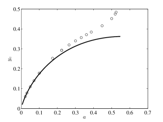
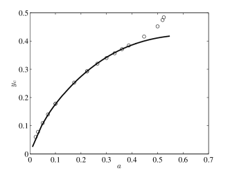
It is often assumed that trap motion improves capture time ([34, 35, 36]). Using two simple examples (oscillatory and random trap motion), we have shown that when finite domains are considered, this may not always the case: a mobile trap can lead to a slower capture time if its mobility is sufficiently low. In particular, for a trap located at the center of the domain, we find that undergoing random motion impairs its capture time if the motion is not sufficiently fast (more than $0.53$ times the speed of the particle). For a trap under prescribed motion oscillating with small amplitude about the center of the domain, the effect of motion on the average MFPT also depends on the mobility of the trap: a mobile trap leads to a higher average MFPT when its oscillation frequency $\omega$ is less than some critical frequency $\omega_{c}\approx 9.6017$. When the oscillation amplitude is not small, the dependence of $\omega_{c}$ on the amplitude is shown Figure 3(b), where the individual points were computed from full numerical solutions of (1.3). The increasing behavior of $\omega_{c}$ with $\varepsilon$ reflects the fact that the more the trap deviates from its optimal location at the center of the domain, the faster it needs to move in order recover to the center sufficiently quickly. Observe that for $\varepsilon$ small, $\omega_{c}\sim 9.6017$.

We also showed a surprising connection between the MFPT problem with oscillating interior trap and the frequency of oscillations in spike position for the Gray-Scott model. In particular, we showed that the critical and bifurcation frequency in the respective problems are identical. By showing this equivalence, we were able to prove the existence and uniqueness of a Hopf bifurcation in a particular limit of the Gray-Scott model.

The existence of a critical oscillation frequency in Problem A might suggest a similar type of behavior when considering the problem of splitting probability in the presence of a stationary and oscillatory trap. However, we show briefly here that in the limit of small oscillation amplitude, the random walker is always more likely to become trapped by the mobile trap instead of the stationary one. This problem consists of a trap at the right boundary whose position is given by $\xi\left(t\right)=\frac{1}{2}+\varepsilon\sin(\omega t)$, $\varepsilon\ll 1$, and a stationary trap at $x=0$ on the left. By analogy to the derivation for the MFPT problem (1.1), and that given in [37], we obtain the ODE for the (rescaled) splitting probability

$$u_{t}+u_{xx}=0\,;$$ (5.1a)

$$u(0,t)=1\,,\quad u\left(1/2+\varepsilon\sin\left(\omega t\right),t\right)=0\,,\quad u(x,0)=u(x,2\pi/\omega)\,.$$ (5.1b)

In (5.1), $u(x,t)$ gives the probability that a random walker starting at location $x$ at time $t<2\pi/\omega$ gets captured by the stationary trap located at $x=0$. We find that the average of this probability over one period of trap oscillation, given by

$$\bar{u}=\frac{\omega}{\pi}\int_{0}^{\frac{2\pi}{\omega}}\int_{0}^{1/2+\varepsilon\sin(t\omega)}\!u(x,t)\,dxdt\,,$$ (5.2)

is less than $1/2$ for any $\omega$. Indeed, using a computation similar to that performed in §2, we find that

$$\bar{u}=\frac{1}{2}+\varepsilon^{2}\left\{1-\sqrt{i\omega}\coth\left(\sqrt{i\omega}/2\right)-\sqrt{-i\omega}\coth\left(\sqrt{-i\omega}/2\right)\right\}\,,\qquad\varepsilon\ll 1\,.$$ (5.3)

It is immediate from the identity (2.13) that the term in (5.3) proportional to $\varepsilon$, which accounts for the small amplitude oscillation of the right-hand trap, is negative for all $\omega$. We thus conclude that, in the limit of small amplitude oscillations, the mobile trap is more likely to capture the random walker than the stationary trap on the opposite side, regardless of $\omega$ (unlike Problem A, which exhibited a threshold behaviour in $\omega$). Numerical solutions of (5.1) with $\varepsilon=\mathcal{O}(1)$ suggest that the same conclusion also holds for $\mathcal{O}(1)$ amplitude oscillations.

An interesting problem would be to see if the equivalence between Problems A and C carries over to two or more dimensions. The derivation of (1.1) for the MFPT extends easily to higher dimensions, and thus may also be employed to formulate PDE’s for the MFPT in the presence of general trap motion and domain geometry. This allows for a full investigation of MFPT problems with mobile traps by way of either numerical computations or asymptotic analysis. Such a study has not yet been carried out.

Another interesting problem would be to replace the sinusoidal trap motion in Problem A by a general periodic $f(t)$ with the same period and amplitude. This analysis could be done by writing $f(t)$ in terms of its Fourier series. An optimization problem may be then be posed by asking what $f(t)$ minimizes average MFPT, while penalizing the average square velocity of the trap. In practice, this type of problem lends to situations where reduced capture times must be weighed against higher energy expenditure, for example, in predator search strategy.

Appendix A Derivation of Problem C

We begin with the Gray-Scott model as scaled in [38]:

$$v_{t}=\varepsilon^{2}v_{xx}-v+Auv^{2}\,,\qquad v_{x}(0,t)=v_{x}(1,t)=0\,,$$ (A.1a)

$$\tau u_{t}=Du_{xx}+1-u-\frac{uv^{2}}{\varepsilon}\,,\qquad u_{x}(0,t)=u_{x}(1,t)=0\,,$$ (A.1b)

supplemented by appropriate initial conditions. In the limit $\varepsilon\to 0$, it is shown that (A.1) admits a single spike solution whose dynamics are given by the reduced system

$$u_{t}=Du_{xx}+1-u-\frac{6}{A^{2}u_{0}}\,\delta\left(x-\xi\right)\,;\qquad\xi_{t}=\frac{\tau\varepsilon^{2}}{u_{0}}\left(u_{x}(\xi^{+}(t),t)+u_{x}(\xi^{-}(t),t)\right)\,,$$ (A.2)

where $u_{0}=u(\xi(t),t)$. In (A.2), $\xi(t)$ represents the location of the center of the spike. We assume that $A\gg 1$ in (A.2) and make a change of variables

$$u=1+\frac{\hat{u}}{A^{2}}\,.$$ (A.3)

With (A.3) in (A.2), the leading order terms yield

$$\hat{u}_{t}=D\hat{u}_{xx}-\hat{u}-6\delta\left(x-\xi\right)\,;\qquad\xi_{t}=\frac{\tau\varepsilon^{2}}{A^{2}}\left(\hat{u}_{x}^{+}+\hat{u}_{x}^{-}\right)\,.$$ (A.4)

Next, we suppose that $D\gg 1$ and make the final change of variables in (A.4)

$$\hat{u}=6\left(-1+\frac{\tilde{u}}{D}\right)\,,\qquad t=\hat{t}/D\,,\qquad\beta=\frac{6\tau\varepsilon^{2}}{A^{2}D^{2}}\,.$$

The resulting leading-order expression becomes precisely (1.5) upon dropping the hats.

Appendix B Next order term for computation of $y_{c}$

A more accurate formula for $y_{c}$ can be obtained by keeping all terms from (3.12a) in (3.13). In particular this requires the full computation of $V_{2}$ in (3.10). Substituting (3.10) for $U_{2}$ into (3.8c), we obtain the equation for $V_{2}$

$$V_{2xx}+V_{2\eta\eta}=0\,;\qquad V_{2}(0,\eta)=f(\eta)\,,\quad V_{2x}(1,\eta)=0\,,\quad V_{2\eta}(x,0)=0\,,\quad V_{2}\to 0\enspace\mbox{as}\enspace\eta\to\infty\,.$$ (B.1)

In (B.1), $f(\eta)$ is defined as

$$f(\eta)\equiv\eta\sum_{n=0}^{\infty}{\frac{2}{\lambda_{n}}e^{-\lambda_{n}\eta}}\,.$$ (B.2)

To solve (B.1), we use a Fourier cosine transform and its inverse defined by

$$\hat{G}(x,\omega)=4\int_{0}^{\infty}\!g(x,\eta)\cos(2\pi\omega\eta)\,d\eta\,,\qquad g(x,\eta)=\int_{0}^{\infty}\!\hat{G}(x,\omega)\cos(2\pi\omega\eta)\,d\omega\,.$$

Proceeding, we calculate that

$$V_{2}=\int_{0}^{\infty}\!\frac{\hat{F}(\omega)}{\cosh(2\pi\omega)}\cosh(2\pi\omega(x-1))\cos(2\pi\omega\eta)\,d\omega\,,$$ (B.3)

where $\hat{F}(\omega)$ is the Fourier cosine transform of $f(\eta)$ in (B.2). The resulting expression for $u_{m}(x,y;a)$, accurate to $\mathcal{O}(a^{2})$, is then given by (3.12b) with $V_{2}(x,y/a)$ given by (B.3). The condition that $u_{m}(x,y;a)$ integrates to $0$ in (3.3) then yields the condition for $y_{c}$,

$$-\sum_{n=0}^{\infty}{\frac{2}{\lambda_{n}^{3}}e^{-\lambda_{n}y_{c}/a}\cos(\lambda_{n}y_{c})}+a\left[(y_{c})^{2}-y_{c}+\frac{1}{3}\right]+\\ +a\int_{0}^{\infty}\!\frac{\hat{F}(\omega)}{2\pi\omega\cosh(2\pi\omega)}\sinh(2\pi\omega(x-1))\cos(2\pi\omega y_{c}/a)=0\,.$$ (B.4)

Solving (B.4) numerically for $y_{c}$, we obtain the solid curve in Figure 5(b). Note that, in comparison to Figure 5(a), which contains the leading order expression for $y_{c}$ in (3.4), we observe a larger range of agreement between the asymptotic and numerical (open circles) results.

References

- [1] Z. Schuss, A. Singer, D. Holcman, The narrow escape problem for diffusion in cellular microdomains, Proceedings of the National Academy of Sciences 104 (41) (2007) 16098–16103.
- [2] M. S. Titcombe, M. J. Ward, An asymptotic study of oxygen transport from multiple capillaries to skeletal muscle tissue, SIAM Journal on Applied Mathematics 60 (5) (2000) 1767–1788.
- [3] E. Barkai, D. A. Kessler, Transport and the first passage time problem with application to cold atoms in optical traps, arXiv preprint arXiv:1305.0081 .
- [4] R. Yvinec, M. R. D’Orsogna, T. Chou, First passage times in homogeneous nucleation and self-assembly, The Journal of Chemical Physics 137 (24) (2012) 244107.
- [5] O. Bénichou, M. Coppey, M. Moreau, P. Suet, R. Voituriez, Optimal search strategies for hidden targets, Physical Review Letters 94 (19) (2005) 198101.
- [6] O. Bénichou, C. Loverdo, M. Moreau, R. Voituriez, Intermittent search strategies, Reviews of Modern Physics 83 (1) (2011) 81.
- [7] M. A. Lomholt, T. Ambjörnsson, R. Metzler, Optimal target search on a fast-folding polymer chain with volume exchange, Physical Review Letters 95 (26) (2005) 260603.
- [8] I. M. Sokolov, R. Metzler, K. Pant, M. C. Williams, Target search of N sliding proteins on a DNA, Biophysical Journal 89 (2) (2005) 895–902.
- [9] S. P. Ramanathan, K. Van Aelst, A. Sears, L. J. Peakman, F. M. Diffin, M. D. Szczelkun, R. Seidel, Type iii restriction enzymes communicate in 1d without looping between their target sites, Proceedings of the National Academy of Sciences 106 (6) (2009) 1748–1753.
- [10] L. Mirny, M. Slutsky, Z. Wunderlich, A. Tafvizi, J. Leith, A. Kosmrlj, How a protein searches for its site on DNA: the mechanism of facilitated diffusion, Journal of Physics A: Mathematical and Theoretical 42 (43) (2009) 434013.
- [11] O. Bénichou, Y. Kafri, M. Sheinman, R. Voituriez, Searching fast for a target on DNA without falling to traps, Physical Review Letters 103 (13) (2009) 138102.
- [12] O. Bénichou, R. Voituriez, From first-passage times of random walks in confinement to geometry-controlled kinetics, Physics Reports 539 (4) (2014) 225–284.
- [13] L. Giuggioli, S. Pérez-Becker, D. P. Sanders, Encounter times in overlapping domains: Application to epidemic spread in a population of territorial animals, Physical Review Letters 110 (5) (2013) 058103.
- [14] D. Holcman, I. Kupka, The probability of an encounter of two Brownian particles before escape, Journal of Physics A: Mathematical and Theoretical 42 (31) (2009) 315210.
- [15] V. Tejedor, O. Bénichou, R. Metzler, R. Voituriez, Residual mean first-passage time for jump processes: theory and applications to Lévy flights and fractional Brownian motion, Journal of Physics A: Mathematical and Theoretical 44 (25) (2011) 255003.
- [16] J. C. Tzou, T. Kolokolnikov, Mean first passage time for a small rotating trap inside a reflective disk, arXiv preprint arXiv:1405.2302 .
- [17] D. Toussaint, F. Wilczek, Particle–antiparticle annihilation in diffusive motion, The Journal of Chemical Physics 78 (5) (1983) 2642–2647.
- [18] S. A. Rice, Diffusion-limited reactions, Elsevier, 1985.
- [19] P. Hänggi, P. Talkner, M. Borkovec, Reaction-rate theory: fifty years after Kramers, Reviews of Modern Physics 62 (2) (1990) 251.
- [20] A. Szabo, R. Zwanzig, N. Agmon, Diffusion-controlled reactions with mobile traps, Physical Review Letters 61 (21) (1988) 2496.
- [21] N. Komarov, P. Winkler, Capturing the drunk robber on a graph, arXiv preprint arXiv:1305.4559 .
- [22] G. Oshanin, O. Vasilyev, P. Krapivsky, J. Klafter, Survival of an evasive prey, Proceedings of the National Academy of Sciences 106 (33) (2009) 13696–13701.
- [23] G. Oshanin, O. Bénichou, M. Coppey, M. Moreau, Trapping reactions with randomly moving traps: Exact asymptotic results for compact exploration, Physical Review E 66 (6) (2002) 060101.
- [24] A. Gabel, S. N. Majumdar, N. K. Panduranga, S. Redner, Can a lamb reach a haven before being eaten by diffusing lions?, Journal of Statistical Mechanics: Theory and Experiment 2012 (05) (2012) P05011.
- [25] A. Kehagias, D. Mitsche, P. Prałat, Cops and invisible robbers: The cost of drunkenness, Theoretical Computer Science 481 (2013) 100–120.
- [26] V. Kurella, J. C. Tzou, D. Coombs, M. J. Ward, Asymptotic analysis of first passage time problems inspired by ecology .
- [27] P. C. Bressloff, J. M. Newby, Stochastic models of intracellular transport, Reviews of Modern Physics 85 (1) (2013) 135.
- [28] J. E. Fletcher, S. Havlin, G. H. Weiss, First passage time problems in time-dependent fields, Journal of Statistical Physics 51 (1-2) (1988) 215–232.
- [29] J. J. Brey, J. Casado-Pascual, First passage time problems and resonant behavior on a fluctuating lattice, Physica A: Statistical Mechanics and its Applications 212 (1–2) (1994) 123 – 131.
- [30] J. A. Revelli, C. E. Budde, H. S. Wio, Diffusion in fluctuating media: resonant activation, Physica A: Statistical Mechanics and its Applications 342 (1) (2004) 1–8.
- [31] A. K. Dhara, T. Mukhopadhyay, Coherent stochastic resonance in one dimensional diffusion with one reflecting and one absorbing boundaries, Journal of Statistical Physics 107 (3-4) (2002) 685–703.
- [32] B. Dybiec, E. Gudowska-Nowak, Resonant activation in the presence of nonequilibrated baths, Physical Review E 69 (1) (2004) 016105.
- [33] A. S. Pikovsky, J. Kurths, Coherence resonance in a noise-driven excitable system, Physical Review Letters 78 (5) (1997) 775.
- [34] R. Blythe, A. Bray, Survival probability of a diffusing particle in the presence of Poisson-distributed mobile traps, Physical Review E 67 (4) (2003) 041101.
- [35] M. Moreau, G. Oshanin, O. Bénichou, M. Coppey, Pascal principle for diffusion-controlled trapping reactions, Physical Review E 67 (4) (2003) 045104.
- [36] M. Moreau, G. Oshanin, O. Bénichou, M. Coppey, Lattice theory of trapping reactions with mobile species, Physical Review E 69 (4) (2004) 046101.
- [37] S. Redner, A guide to first-passage processes, Cambridge University Press, 2001.
- [38] W. Chen, M. J. Ward, Oscillatory instabilities and dynamics of multi-spike patterns for the one-dimensional Gray-Scott model, European Journal of Applied Mathematics 20 (02) (2009) 187–214.
- [39] C. B. Muratov, V. Osipov, Stability of the static spike autosolitons in the Gray–Scott model, SIAM Journal on Applied Mathematics 62 (5) (2002) 1463–1487.
- [40] C. Muratov, V. Osipov, Static spike autosolitons in the Gray-Scott model, Journal of Physics A: Mathematical and General 33 (48) (2000) 8893.
- [41] A. Doelman, T. J. Kaper, P. A. Zegeling, Pattern formation in the one-dimensional Gray-Scott model, Nonlinearity 10 (2) (1997) 523.
- [42] T. Kolokolinikov, M. J. Ward, J. Wei, Slow translational instabilities of spike patterns in the one-dimensional Gray-Scott model, Interfaces and Free Boundaries 8 (2) (2006) 185.
- [43] V. Tejedor, M. Schad, O. Bénichou, R. Voituriez, R. Metzler, Encounter distribution of two random walkers on a finite one-dimensional interval, Journal of Physics A: Mathematical and Theoretical 44 (39) (2011) 395005.