SIR model on a dynamical network and the endemic state of an infectious disease

Abstract

In this work we performed a numerical study of an epidemic model that mimics the endemic state of whooping cough in the pre-vaccine era. We considered a stochastic SIR model on dynamical networks that involve local and global contacts among individuals and analyzed the influence of the network properties on the characterization of the quasi-stationary state. We computed probability density functions (PDF) for infected fraction of individuals and found that they are well fitted by gamma functions, excepted the tails of the distributions that are q-exponentials. We also computed the fluctuation power spectra of infective time series for different networks. We found that network effects can be partially absorbed by rescaling the rate of infective contacts of the model. An explicit relation between the effective transmission rate of the disease and the correlation of susceptible individuals with their infective nearest neighbours was obtained. This relation quantifies the known screening of infective individuals observed in these networks. We finally discuss the goodness and limitations of the SIR model with homogeneous mixing and parameters taken from epidemiological data to describe the dynamic behaviour observed in the networks studied.

Keywords: SIR; network; stochastic; pertussis

¹ e-mail: fabricius@fisica.unlp.edu.ar (corresponding author)

1 Introduction

Mathematical modelling of infectious diseases is an interdisciplinary area of increasing interest. Since the pioneering work of Kermack and McKendrick [1], mathematical modelling has shown to be a powerful tool to understand infectious disease transmission [2, 3, 4, 5]. The fact that the simple deterministic SIR model, where the population is divided into susceptible (S), infective (I) and immune or recovered (R) individuals, is able to predict quite well the outbreak periods for a large series of infectious diseases in many countries around the world suggests that it captures the essentials of transmission dynamics [2]. Lately, models gained an increasing level of complexity, including age structure and particular features of the given disease, with the aim of being more realistic and predictive [2, 6, 7, 8]. Due to the complexities of these models, stochastic effects and the network structure of contacts are rarely considered. However, when considered (in much more simple models) stochastic effects have shown to play an important role in understanding the data of reported cases of measles and pertussis [9]. More recently, the effect of the network structure of contacts on the disease transmission has been considered in several publications, always in models with very few epidemiological classes [10, 11, 12, 13]. In particular, in Refs. [14, 15] the authors studied the spatial correlations and stochastic fluctuations using SIR and SEIR models on two-dimensional Watts-Strogatz-type dynamical networks. Simöes et al. [15] focussed on the power spectrum of the fraction of infective time series and performed an extensive study of parameter space for the SIR model. They found that spatial correlations and the deterministic recovery of infection increase the amplitude and coherence of the resonant stochastic fluctuations and studied the dependence of such changes on model parameters.

In the present work, we use the SIR stochastic model on two-dimesional Watts-Strogatz-type dynamical networks and perform an intensive study of the model for parameters corresponding to pertussis disease (whooping cough) in the pre-vaccine era. We carry out simulations for different parameters characterizing the network properties and study their influence on the behaviour of the quasi-stationary state of the system corresponding to the endemic disease with periodic outbreaks. The purpose of our work is twofold. On the one hand, we assume the disease is propagating in a place with a well-mixed population, and then, for some reason, the network of contacts changes and becomes more local. We analyzed the consequences of this change in disease transmission. On the other hand, we focus on a methodological point. Suppose the disease is propagating in a city where local contacts are important, but a SIR stochastical model disregarding network structure is used. How bad is the description of the problem in this case if you parametrize the model to available epidemiological data?

2 Model and simulations

We consider a stochastic SIR model on Watts-Strogatz dynamic-type networks as the ones studied by Verdasca et al. [14] and Simöes et al. [15]. Our setup of the model is summarized below. First, we describe the underlying SIR deterministic model with births and deaths.

2.1 Deterministic SIR model

In this model it is assumed that individuals are in one of the following three epidemiological classes: susceptible, infected or recovered. Individuals are born in a susceptible class at a rate $\mu$ and they remain there until they become infected by contact with an infected individual. Infected individuals recover from infection entering the recovered class at a rate $\gamma$. The dynamic variables of the model are the fractions of the population in each epidemiological class, and they obey the following set of non-linear coupled differential equations:

$$\frac{ds}{dt}=-\beta si+\mu-\mu s$$

$$\frac{di}{dt}=\beta si-\gamma i-\mu i$$ (1)

$$\frac{dr}{dt}=\gamma i-\mu r$$

where $s$, $i$ and $r$ are the fractions of people in susceptible, infected and recovered classes respectively. In this model the term $\beta si$ represents the incidence per individual of the disease (the rate at which susceptible individuals become infected) and contains the key approximation of the model: uniform mixing. Parameter $\beta$ is the rate of infective contacts (which are the contacts such that if one individual is infected and the other susceptible, the latter will become infected). So, in the uniform mixing approximation it is assumed that all susceptible individuals become infected at the same rate: $\beta i$. In this model the death rate is assumed equal for people in the three epidemiological classes and also equal to the birth rate, $\mu$, in order to keep the population constant.

The set of differential equations 1 determines the dynamic evolution of the system. For any initial conditions different from i=0 (when the system goes towards the fixed point: $s=1$, $i=0$, $r=0$), the system asymptotically reaches the stationary state: $s=s^{*}=(\gamma+\mu)/\beta$, $i=i^{*}=\mu/(\gamma+\mu)(1-s^{*})$, $r^{*}=1-s^{*}-i^{*}$.

2.2 Stochastic model on the network

We consider N individuals on a squared lattice (LxL=N) with periodic boundary conditions. At each site there is an individual that may be in one of the 3 epidemiological states: S (suscepible), I (infected) or R (recovered). The state of an individual at site $j$ is a stochastic variable of the model, $X_{j}$, that may change through the following processes:

$$infection: S\rightarrow I$$

$$recovering: I\rightarrow R$$

$$death\ and\ birth: S\rightarrow S$$

$$I\rightarrow S$$

$$R\rightarrow S$$

We assume that when an individual dies at a site, another individual is born at the same time at this site in order to keep every site with one individual during the simulation. As we suppose Markovian processes, the dynamics of the system is controlled by the knowledge of probability transition rates at each time. Deaths and births are independent of the individual state and occur at the same probability rate $\mu$. To account for infections we consider a dynamic type of Watts-Strogatz network [16]. We assume that, at a given time, an individual at site $j$ has contact with a randomly chosen individual in the network with probability rate $p\beta$, and with one of their $k$ nearest neighbours with probability rate $(1-p)\beta$. If the individual at site $j$ is susceptible, and the contacted individual is infected, then the individual at site $j$ will become infected. Local contacts of an individual represent the contacts with known people (in the circle of their stable relations) while global random contacts represent people met by chance (for example, on a bus, shopping, etc). Actually, here the word “contact” is restricted to “infective contacts”, in the sense discussed above for the SIR model. The model used in the present work allows changing the degree of “locality” of the network by changing the value of parameter $p$. In particular, for $p=0$ an individual only has contacts with their $k$ nearest neighbours while for $p=1$ an individual may contact any other individual in the lattice with the same probability as in the classical stochastic SIR model (uniform mixing). This is an important difference with the standard (static) Watts-Strogatz setting [16] where the case $p=1$ corresponds to a random network where an individual has a fixed number $k$ ($<<$N) of random contacts. Recovery from infection is the same in every site and occurs at a probability rate $\gamma$. This assumption gives exponentially distributed recovery times, which is a reasonable approximation for pertussis [17].

In summary, the probability transition rates for infection, recovery and death-birth processes at site “$j$” are

$$a_{inf}^{j}=\left[p\ \beta\ i+(1-p)\beta\ \frac{1}{k}\sum_{j^{\prime}\in\nu_{j}}\delta_{X_{j^{\prime}},I}\right]\delta_{X_{j},S}$$

$$a_{rec}^{j}=\gamma\delta_{X_{j},I}$$ (2)

$$a_{d-b}^{j}=\mu$$

where $\delta_{AB}$ is one if states $A$ and $B$ are the same, and zero if not. $X_{j}$ is the state of the individual at site $j$, and $j^{\prime}$ in the sum runs over the $k$ neighbours of site $j$ (we call this set of sites $\nu_{j}$).

The probability rate for infections, recoveries or death-birth processes in the whole system is obtained summing over $j$ in Eqs. 2 and gives

$$a_{inf}=p\ \beta\ i\ s\ N+(1-p)\beta\ n_{SI_{\nu}}N$$ (3)

$$a_{rec}=\gamma iN$$ (4)

$$a_{d-b}=\mu N$$ (5)

where $i$ and $s$ are the fractions of infected and susceptible individuals in the system, and $n_{SI_{\nu}}$ is given by

$$n_{SI_{\nu}}=\frac{1}{N}\sum_{j=1}^{N}\frac{1}{k}\sum_{j^{\prime}\in\nu_{j}}\delta_{X_{j},S}\ \delta_{X_{j^{\prime}},I}$$ (6)

In the case $p=1$ and $N\rightarrow\infty$, for $i$ and $s$ the stochastic model gives the same dynamics as that of the deterministic Eqs. 1. For $p<1$ the dynamics will be affected by the correlation among susceptible and infected neighbours explicitely included in the term: $n_{SI_{\nu}}$.

2.3 Simulation algorithm

The state of the system at a given time $t^{\alpha}$ is specified by the knowledge of the $N$ variables $X^{\alpha}_{j}$: ${\bf X^{\alpha}}=(X^{\alpha}_{1},X^{\alpha}_{2},...,X^{\alpha}_{N})$. We perform stochastic simulations using Gillespie algorithm [18]. This is an exact algorithm that generates a Markov chain for the master equation that could be constructed from the probability rates given in Eqs. 2. The algorithm gives a sequence of times $t^{1}$, $t^{2}$, … and the corresponding states ${\bf X^{1}}$, ${\bf X^{2}}$, …, where two consecutive states differ by a single process that occurs at a given site. The process and the time when it takes place are generated from simple rules and two random numbers (see Ref. [18] for details). As the probabiliy rates are functions of the stochastic variables of the model, they are changed at each step of the simulation.

2.4 Average computation

For each system to be studied we generate a set of $M$ Markov chains, from specified initial conditions, and use different sets of random numbers, checking that each trajectory survives at least a time $t_{run}$. We denote the state of the system corresponding to Markov chain m at time $t^{\alpha}$: ${\bf X_{m}^{\alpha}}$. To compute the average of an observable $A\left[{\bf X_{m}^{\alpha}}\right]$ over the $M$ samples at a given time, we take into account that the set of discrete times $t^{1}$, $t^{2}$, …, $t^{\alpha}$,… will be different for each one of the m=1, …,$M$ trajectories. So, we define

$$\left<A(t)\right>=\frac{1}{M}\sum_{m=1}^{M}A_{m}(t),\ \ A_{m}(t)=\left(A\left[{\bf X_{m}^{\alpha}}\right]+A\left[{\bf X_{m}^{\alpha+1}}\right]\right)/2$$ (7)

with $t^{\alpha}<t<t^{\alpha+1}$. As $t^{\alpha+1}-t^{\alpha}$ is the time interval between 2 single processes, it is much shorter than the time taken by the whole system to undergo a detectable change.

Similarly, we define the time correlation of an observable at two diferent times

$$\left<A(t^{\prime})A(t^{\prime\prime})\right>=\frac{1}{M}\sum_{m=1}^{M}A_{m}(t)A_{m}(t^{\prime})$$ (8)

The main observable studied in the present work is the fraction of infected individuals

$$i\left[{\bf X_{m}^{\alpha}}\right]=\frac{1}{N}\sum_{j=1}^{N}\delta_{{\bf X_{m}^{\alpha}}_{j},I}$$ (9)

3 Results

We perform simulations using the algorithm described in sections 2.2 and 2.3 for L=800 (which corresponds to a city of N=640,000 inhabitants) and consider diferent networks corresponding to the cases $k$= 4, 8 and 12, including up to first, second and third neighbours respectively, and $p$ varying from 1.0 to 0.2. We take $\mu=1/(50$ years), $\gamma=1/(21$ days) and $\beta=0.8$ 1/day, which are standard parameters for SIR description of pertussis in pre-vaccine era [19]. When other $\beta$ values are used in the simulations, it is mentioned explicitely.

3.1 The quasi-stationary state

3.1.1 Definition and empirical assumption of its existence

The purpose of this work is to simulate the endemic state of a disease that should be represented by a stationary state of the model. As we mentioned above in the case $p=1$, $N\rightarrow\infty$, the dynamics of the system follows Eqs. 1 and so, for every initial condition with $i\neq 0$ the stationary state $(s^{*},i^{*})$ is reached. However, for any finite value of $N$ the only stationary state of the system is $s=1,i=0$ because sooner or later a fluctuation will make the number of infected individuals zero, and there is no process that produces infected individuals if there is none in the system. Nevertheless, for N large enough, the system may fluctuate for a long time around a quasi-stationary state (QSS) before extinction. The definition and properties of such a state have been addressed in other contexts from a mathematical point of view [20, 21] or with empirical approaches [22, 23]. In the present work an empirical strategy is developed. There are two points to be considered in order that the system reaches a QSS and remains there long enough to be studied. For $p<1$ the system develops correlations and there is a time needed to arrive at this correlated QSS that depends on the initial conditions. Moreover, the size of the fluctuations (and thereby the probability of extinctions) as well as $N$, depend on the parameters that define network properties: $p$ and $k$. Then, the time window where a QSS of the system could be defined has to be determined with some care.

Estimation of extinction times

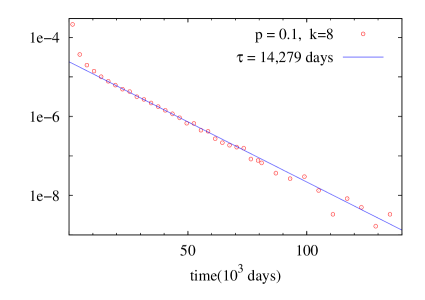
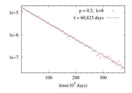
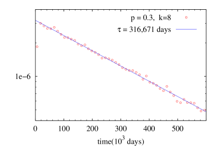
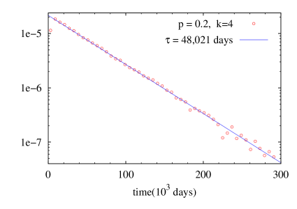
We first calculate the distribution of living times in order to estimate the typical time that the system survives until extintion. We proceed as follows: (i) for each ($k,p$) network we perform several runs and, from those that survive long enough, we obtain approximate values for the average number of susceptible, infected and recovered individuals, (ii) as an initial condition for our study, in the network sites we randomly distribute a number of S, I and R individuals as obtained in (i), (iii) we generate M=50,000 different samples as in (ii) (100,000 for $p=0.1$) and let each sample evolve until extinction, (iv) we compute the fraction of the samples that extinguished in interval $(t,t+\Delta t)$. The results are shown in Fig.1. In all cases considered exponentials fit quite well the results of simulations. For the SIR stochastic model I. N$\mathring{{\rm a}}$ssel [21] has proved that extinction times have an exponential distribution as we found here numerically for a more complex model and other initial conditions. The typical time of extinction decreases sharply with $p$. It is reduced to $1/20$ of its value in going from $p=0.3$ to $p=0.1$ for $k=8$. Extinction times also decreases when lowering $k$ but the effect is weaker, for example, they undergo only a 20% reduction when the neighbours are reduced from $k=8$ to $k=4$, for $p=0.2$.

(a)

(b)

(c)

(d)

Figure 1: Distribution of living times for different networks. The points indicate the fraction of the samples considered extinguished at a given time per unit of time. The continuous lines are exponential fits $C\exp(-t/\tau)$ to the data. The fitted value of $\tau$ is shown in each figure.

Estimation of equilibration times

Figure 2 shows the time evolution of $\left<i(t)\right>$ computed averaging over $M$=20,000 samples that survive at least a time $t_{run}=40,000$ days. The initial conditions for the simulations are generated as in (ii).

Figure 2: Average fraction of infected individuals $\left<i(t)\right>$ as a function of time for networks with $k=8$ and different $p$-values. The average is performed over $M$=20,000 samples for each case.

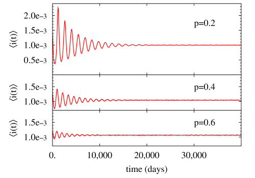
After a time that is longer for lower $p$, $\left<i(t)\right>$ remains around a constant value that we take as the stationary value of $\left<i(t)\right>$ and denote it: $\left<i\right>$. For $t>20,000$ days, the curves of Fig.2 verify $|\left<i(t)\right>-\left<i\right>|<\epsilon$=0.00001, where $\left<i\right>$ is 0.001, 0.00104 and 0.00106 for $p$=0.2, 0.4 and 0.6, respectively. As the fraction of infective individuals in the system is the more fluctuating magnitude we have studied, we assume its constancy in time is a sufficient condition to define the quasi-stationary state of the system. The longer time needed to arrive at QSS as $p$ decreases is related to the increasing time needed for the network to establish local correlations. In particular, for the case $p$=1 (not shown in the figure) the system is at QSS from t=0. Taking the time window $(t_{a},t_{b})$, $t_{a}$=20,000 days, $t_{b}=$40,000 days, the 20,000 samples that survive 40,000 days for $p$=0.2 represent a significant 52% of the generated samples. Conversely, in the case $p$=0.1 for $t=$20,000, when QSS has not been reached yet, only 8% of the samples survive. As in this work we are interested in the study and characterization of the endemic state of the disease, we haven’t considered networks where the probability of establishment and survival of the steady state is very low. In the present work we consider values of $p\geq 0.2$.

In summary, for each network ($k$, $p$) considered we obtained a number $M$=20,000 of Markov chains generated from independent samples of the system that survive at least a time $t_{b}=$40,000 days. In the time window $(t_{a},t_{b})$ the magnitudes of interest remain stationary within an acceptable precision ($\epsilon$) when averaged over the $M$ samples. From this empirical fact we assume the existence of a quasi-stationary state and that each one of the $M$ trajectories ${\bf X_{m}^{\alpha}}$ (m=1,..M) represents a possible time evolution of the disease in the endemic state ($t_{a}<t^{\alpha}<t_{b}$). The stationary value of an observable average $\left<A(t)\right>$ will be denoted $\left<A\right>$. In particular, for the fraction of infected or susceptible individuals in the system

$$\left<i(t)\right>=\left<i\right>,\ \left<s(t)\right>=\left<s\right>,~{}~{}{\rm for}\ t\in(t_{a},t_{b})$$ (10)

where the equality with the numerical values $\left<i\right>$ and $\left<s\right>$ has to be understood to be valid within the precision $\epsilon$.

3.1.2 Relation between $\left<s\right>$ and $\left<i\right>$

In a given state ${\bf X^{\alpha}}$, the expected change in the fraction of infected individuals in the system is governed by the net probabilty rate

$$\left(a_{inf}[{\bf X^{\alpha}}]-a_{rec}[{\bf X^{\alpha}}]-i\ a_{d-b}[{\bf X^{\alpha}}]\right)/N$$ (11)

but stationarity of $\left<i(t)\right>$ implies

$$\left<a_{inf}\right>-\left<a_{rec}\right>-\left<i\ a_{d-b}\right>=0\Rightarrow\left<a_{inf}\right>/N=(\gamma+\mu).\left<i\right>$$ (12)

where we have taken $a_{rec}=\gamma i$ and $a_{d-b}=\mu$ from Eqs. 4 and 5. In the same way, the stationarity of $\left<s(t)\right>$ gives

$$-\left<a_{inf}\right>+\left<a_{d-b}\right>-\left<s\ a_{d-b}\right>=0\Rightarrow\left<a_{inf}\right>/N=\mu.(1-\left<s\right>)$$ (13)

From Eqs. 12 and 13

$$\left<i\right>=\frac{\mu}{\gamma+\mu}.(1-\left<s\right>)$$ (14)

i.e., $\left<s\right>$ and $\left<i\right>$ should be related by the same relation as that of $s^{*}$ and $i^{*}$ in the deterministic model, independently of the average rate of production of infective individuals in the system, controlled by $\left<a_{inf}\right>$.

3.2 Stationary behaviour

In Fig. 3 we show the stationary values of susceptible and infected fractions of individuals for all the networks considered.

Figure 3: Stationary values of susceptible and infected fractions in the network as a function of $p$ for a different number of neighbours $k$.

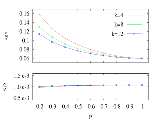
While $\left<s\right>$ increases as $p$ and $k$ decrease, $\left<i\right>$ remains almost constant. For the case p=0.2, k=4, $\left<s\right>$ is 2.6 times larger than for $p=1$ while $\left<i\right>$ decreases only by 10%. The curves $\left<i\right>$ vs. $\left<s\right>$ (not shown) satisfy Eq. 14 within the precision of our simulations for the 27 ($k$, $p$) networks considered. Given the $\left<s\right>$ dependence on $p$ and $k$ shown in Fig.3, a much weaker dependence of $\left<i\right>$ on network parameters is in fact predicted by Eq. 14, since $\left<s\right>$ is always small compared with 1, and $\left<i\right>$ depends on network parameters through the factor $(1-\left<s\right>)$.

The increase of $\left<s\right>$ when the locality of the network increases is a consequence of the decrease in effective transmission of the disease. To quantify disease transmission in the network, we define the effective transmission rate

$$\beta_{eff}=\frac{\left<a_{inf}\right>/N}{\left<i\right>\left<s\right>}$$ (15)

as the mean rate of infections per individual in the network, divided by the stationary values of fractions of infected and susceptible individuals. With this definition the average production of infections in the system is connected with $\left<s\right>$ and $\left<i\right>$ by the uniform mixing expression: $\beta_{eff}$N$\left<s\right>$$\left<i\right>$, $\beta_{eff}$ playing the role of a “global effective” contact rate in a problem where local and global contacts are present.

In Fig. 4 we show $\beta_{eff}$ for all the networks considered.

Figure 4: Effective transmission rate $\beta_{eff}$ as a function of $p$ for a different number of neighbours $k$.

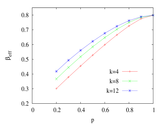
Transmission of the disease in the network decreases with $p$ and $k$ as the network becomes more local. The drop in transmission with $p$ has been related to the clustering of susceptible and infected individuals that is produced by local correlations [14, 15]. This clustering would reduce the probability of finding $I-S$ neighbours and the local contribution to transmission. In order to make the connection between disease transmission and local correlations quantitative, we express $\beta_{eff}$ as

$$\beta_{eff}=\beta+p\beta\frac{C_{si}}{\left<i\right>\left<s\right>}+(1-p)\beta\frac{C_{SI_{\nu}}}{\left<i\right>\left<s\right>}$$ (16)

in terms of the correlation coefficients

$$C_{si}=\left<si\right>-\left<i\right>\left<s\right>,\ \ C_{SI_{\nu}}=\left<n_{SI_{\nu}}\right>-\left<i\right>\left<s\right>$$ (17)

where we have taken the average of Eq. 3 to replace $\left<a_{inf}\right>$ in Eq. 15. Correlation $C_{si}$ measures the average fluctuation of the product of the fractions of susceptible and infected individuals in the population, while $C_{SI_{\nu}}$ is a measure of the local correlation between $S$ individuals with their $I$ neighbours.

(a)

(b)

Figure 5: (a) Correlation coefficients $C_{si}$ and $C_{SI_{\nu}}$ for $k=8$ networks as a function of $p$. (b) The same, but correlations are divided by the product $\left<i\right>$ $\left<s\right>$.

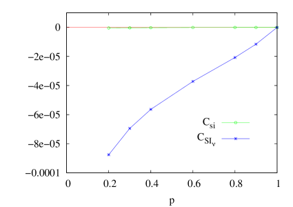
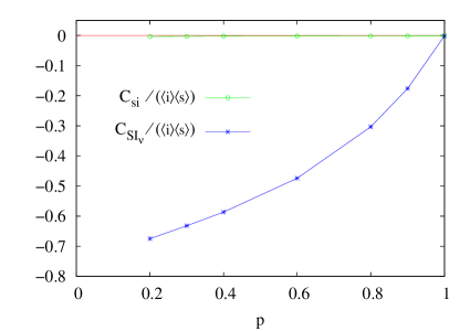
In Fig. 5 we plot both correlations for the case $k=8$. While the magnitude of $C_{si}$ is barely noticeable, $C_{SI_{\nu}}$ indicates that there is a strong reduction in the probability of having S-I pairs of neighbours as p decreases. For $p=1$, $\beta_{eff}$ is almost equal to $\beta$ (the deterministic value) because the correction introduced by fluctuations is lower than 0.5%. For $p<1$ local correlations introduced by the network are appreciable and cause the fall down in $\beta_{eff}$. The definition we take for $\beta_{eff}$ (Eq. 15) and Eq. (12) imply that

$$\left<s\right>=\frac{\gamma+\mu}{\beta_{eff}}$$ (18)

This relation holds for all the networks independently of $p$ and $k$. If we take $\beta_{eff}$ values from Fig. 4 and compute $\left<s\right>$ through Eq. 18, we obtain a set of curves that collapse with those in Fig. 3 (upper panel) validating numerically Eq. 18.

In summary, the relations among stationary values and model parameters for the SIR deterministic model hold exactly the same for the averages at the QSS of the SIR stochastic model in all the networks considered if the rate of infective contacts, $\beta$, is replaced by the effective transmission rate, $\beta_{eff}$. That is, it is possible to account for all the network effects on stationary averages by the rescaling of a single parameter.

3.3 Dynamic behaviour and fluctations

In this section we focus on the dynamic behaviour of the system in the quasi-stationary state. We discuss the case $k$=8 since the other cases considered ($k$=4 and $k$=12) present similar qualitative behaviour. In Fig. 6 we show the time evolution of the fraction of infected individuals for two samples corresponding to networks k=8, p=1, and k=8, p=0.3.

(a)

(b)

Figure 6: Time evolution of the fraction of infected individuals in the QSS for two different samples with $p$=1 (a) and $p$=0.3 (b).

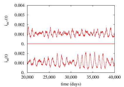
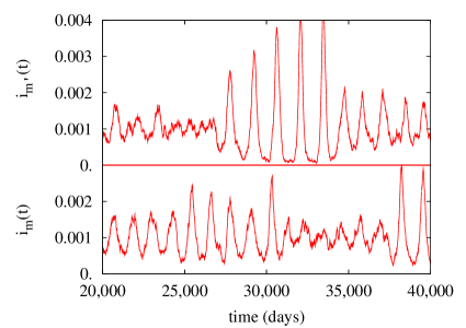
Fluctuations are clearly larger for the case p=0.3 (Fig. 6b) than for $p$=1 (6a). But, the amplitude of fluctuations changes considerably within the time evolution of a given sample. For example, for the case $p$=1 (sample $m$) in the 18 years between t=31,400 days and t=38,000 days (Fig. 6a, lower panel) the amplitude of fluctuations is larger than for case $p$=0.3 (sample $m$) in the 17 years between t=31,000 and t= 37,200 (Fig. 6b, lower panel).

With the aim of characterizing the fluctuations for the networks considered, we compute the probability density functions (PDF), $D(i)$, that are histograms constructed from the instantaneous fractions of infected individuals. In Fig. 7a we show the PDF for networks with $k$=8 and different $p$ values.

(a)

(b)

(c)

(d)

Figure 7: PDF of the fraction of infected individuals, $D(i)$, for networks with $k=8$. (a) $D(i)$ for different values of $p$ parameter. To construct the histograms we use the $M$ trajectories keeping an $i$ value every 10 days. This gives more than $2.10^{7}$ $i-$values per histogram. (b) $\Gamma$-distribution fits (solid lines) to the $D(i)$ of (a) (points). Inset: detail for case $p$=0.3 showing the fit underestimation of the $D(i)$ tail. (c) $q$-exponential fit ($q$=1.04) to the $D(i)$ tail for case $p$=0.3. (d) $D(i)$ for networks with different $p$-values and taking different $\beta$-values in order to obtain the same effective transmission rate: $\beta_{eff}$=0.8.

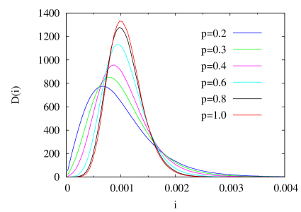
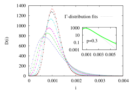
When $p$ decreases, distributions become more asymmetrical with long tails and maxima shifted towards low $i$-values. The combination of both features results in the small variation of $\left<i\right>$ with $p$ that we observed in Fig. 3. The long tails indicate the presence of large peaks of infected individuals as $p$ decreases. We found that PDF are well fitted by $\Gamma$-distributions

$$G(x)=\frac{1}{\Gamma(n)\lambda^{n}}\ x^{n-1}e^{-x/\lambda}$$ (19)

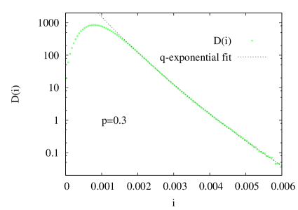
where $\lambda$ and $n$ are the only two fitting parameters. The fits are compared with $D(i)$ histograms in Fig. 7b. The fits are good except for very low and very high values of $i$. The fitted $\Gamma$-distributions underestimate the $D(i)$ tails that fall more slowly than exponentials (see inset of Fig. 7b). In fact, the $D(i)$ tails are well fitted by $q$-exponentials, $Ce_{q}(-\lambda i)$, where

$$e_{q}(x)=\left[1+(1-q)x\right]^{1/(1-q)}$$ (20)

is an exponential in the limit $q\rightarrow 1$ [24]. In Fig. 7c the $D(i)$ tail for case $p=0.3$ is compared with the $q$-exponential fit ($q$=1.04) showing an excellent agreement for three decades of $D(i)$-values.

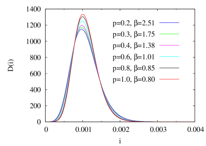
In summary, the study of $D(i)$ distributions reveals a complex behaviour of the instantaneous values of the fraction of infective individuals, $i$, for different networks that is masked by the near constancy of $\left<i\right>$ with $k$ and $p$ observed before. The question that arises at this point is whether this complex behaviour is only due to a change in $\beta_{eff}$. In order to answer this question, we have performed simulations of the system for different networks (different $p$ and $k$ values) but changing the value of parameter $\beta$ in order to obtain the same $\beta_{eff}$ for all cases. In Fig. 7d we show the $D(i)$ distributions for different networks with $k=8$ and the same value of $\beta_{eff}$=0.8. The collapse of the curves for different $p$ values points out that the change in $\beta_{eff}$ was responsible for the main effects of the network on $D(i)$ that we observed in Fig. 7a. However, the collapse of the curves in Fig. 7d is not complete, they are a bit broader for lower $p$ indicating that for the same $\beta_{eff}$, a decrease in $p$ produces slightly larger fluctuations. The change in the mean squared deviation, $\sigma$, and the related change in the peak height are the only relevant differences among these curves that don’t show the large asymmetry of those of Fig. 7a.

To study the dynamical behaviour of the fraction of infective individuals, we compute the self-correlation function

$$c(t)=\left<i(t^{\prime})i(t^{\prime}+t)\right>-\left<i\right>^{2}$$ (21)

which results independent of $t^{\prime}$ in the $(t_{a},t_{b})$ interval. By Fourier transforming $c(t)$, we obtain the power spectrum $P(\omega)=\int\cos(\omega t)c(t)dt$ for the different networks considered (Fig. 8a). As $p$ decreases, the peak of $P(\omega)$ shifts towards lower values of $\omega$ and becomes more pronounced. The area under $P(\omega)$ is proportional to $\sigma^{2}$ [25], indicating that the amplitude of fluctuations increases as $p$ decreases, as could also be inferred from the increasing width of $D(i)$s (Fig. 7a).

(a)

(b)

Figure 8: (a) Fluctuation power spectra of infective time series, $P(\omega)$, for networks with $k=8$ and different $p$-values, (b) $P(\omega)$ for the same networks considered in (a) but taking different $\beta$-values in order to obtain the same effective transmission rate: $\beta_{eff}$=0.8.

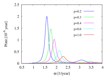
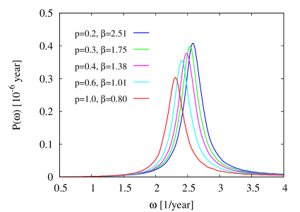
This large increase in $P(\omega)$ peaks when $p$ is reduced, as well as the presence of a secondary harmonic peak have already been observed in a previous study of this system for other model parameters [15]. For the case $p=1$ an analytical expression that approximates very well $P(\omega)$ has been derived [26]. In order to sense how many of the network effects on dynamic correlations can be accounted for by the effective transmission rate, we compute $P(\omega)$ for different networks having the same $\beta_{eff}$. The curves, shown in Fig. 8b, present a slight increase of the peak height as $p$ decreases. The resulting increase in the area under $P(\omega)$ is consistent with the slight increase in width ($\sigma$) of $D(i)$ observed in Fig. 7d. It can be seen that even when $\beta_{eff}$ is kept fixed, there is a shift of the peaks towards greater frequencies as $p$ decreases. These effects depend on the specific set of parameters taken for the SIR model. For example, in Ref. [15] the authors found (for other values of model parameters) that when keeping $\beta_{eff}$ fixed, the height of $P(\omega)$ peak is highly increased when $p$ is lowered, while the shift in frequency is barely noticeable (see Fig. 1c of Ref. [15]).

4 Discussion

Our study of the SIR model on a Watts-Strogatz-type network, for parameters corresponding to pertussis in the pre-vaccine era, shows that network structure strongly influences the disease dynamics. The increasing locality of the network (obtained by lowering $p$) decreases the disease transmission. This effect has already been observed by other authors [14, 15] who attributed it to the clustering of infected individuals produced by local correlations. In the present work we quantified this concept obtaining an explicit relation between the effective transmission rate, $\beta_{eff}$, and correlation coefficients between S and I individuals (Eqs. 16 and 17). An increase in locality also drastically increases fluctuations and the period between outbreaks, which have been analyzed characterizing the probability density functions of fraction of infected individuals, $D(i)$, and the power spectrum of the $i$-time series, $P(\omega)$.

We analyzed whether the network plays another role in the behaviour of the system at the quasi-stationary state besides the change in the effective transmission rate of the disease. Our findings are summarized below:

• The average fractions of susceptible, infected and recovered individuals at the QSS have the same values as in the SIR deterministic model if $\beta$ parameter is replaced by $\beta_{eff}$ of the corresponding network. Therefore, for $\left<s\right>$ and $\left<i\right>$, the network structure may be ignored if a single parameter is changed properly.

• Concerning fluctuations and the time-correlated behaviour of the system, the situation is highly dependent on the SIR-model parameters taken. In particular, if we consider different networks taking the appropiate value for $\beta$ in order to obtain $\beta_{eff}$=0.8, fluctuations in the fraction of infected individuals and their time correlations are very similar as those of the stochastic SIR model ($p=1$) for all the networks considered (Fig. 7d and Fig. 8b). However, network effects are not completely absorbed by $\beta_{eff}$ in this case.

From these remarks we are able to answer the question we raised in the introduction: If we want to describe pertussis transmission in the pre-vaccine era, what is lost if we use a SIR stochastic model with homogenous mixing instead of a SIR stochastic model on the network with determined values of $k$, $p$ and $\beta$? The answer is: very little. In order to parametrize both models, what can be taken from epidemiological data is the basic reproductive ratio $R_{0}$ that, for pertussis in the prevaccine era, is between 16 and 18 [2, 27] and may be obtained from the average fraction of susceptibles, $\left<s\right>$, through the relation: $R_{0}$=1/$\left<s\right>$ [28]. As for the studied systems $\left<s\right>$=$\beta_{eff}$/$(\gamma+\mu)$, epidemiological data fixes $\beta_{eff}$ (not $\beta$) around 0.8. If the SIR stochastic model ($p$=1) is used, the frequency of outbreaks would be a bit underestimated with respect to the prediction of a network with $p<1$ (Fig. 8b). But it would be very difficult to infer the proper $k-p-\beta$ combination from measurable quantities. For example, it is very unlikely that with a power spectrum constructed from a time series of 20 or 30 years it will be possible to choose among one of the curves of Fig. 8b. In fact, given the high heterogeneity in the time series obtained as output of the model (Fig. 6) care should be taken when analyzing real data. If the SIR stochastic model is proposed to describe the dynamics of pertussis in the pre-vaccine era and in cities of the size considered in the present work, the differences observed in the incidence time series in different countries might be due to the heterogeneity of the time profile itself and not to differences in the epidemiological conditions at each place [29]. It would be of great interest to know whether these conclusions may be extended to more complicated and realistic models. In particular, epidemiological and laboratory studies suggest that immunity acquired by pertussis infection is not lifelong (see ref. [30] and references therein) and more realistic models of pertussis transmission include compartments that account for waning immunity [6, 7, 8].

We find it appropriate to emphasize that the results and conclusions obtained in this work hold: a) for the SIR stochastic model in the dynamical networks with local and global contacts as described in section 2.2, b) for the set of parameters used that corresponds to pertussis disease in the pre-vaccine era and c) for the quasi-stationary state of the system, as empirically defined in section 3.1. Extrapolations to other problems that share only some features with the ones treated in the present work are not straightforward and require caution. We expect relations (14), (16) and (18) concerning stationary values to hold independently of the parameters used provided that the quasi-stationary state has been established. But concerning fluctuations we have not obtained general relations and we do not expect that conclusions from the results presented here will be valid for systems with parameters representing other infectious diseases. There are several open questions related to the present work that could be addressed in future research. In particular, it would be interesting to know whether our description of the system at the quasi-stationary state with a beta-rescaled stochastic SIR model could be extended to other model parameters. Moreover, it would be interesting to study whether our description also holds in the approach to the steady state. The problem of constructing mean field approximations to describe the approach and behavior of epidemic systems in the steady state has been studied for the SIRS model on static two-dimensional Watts Strogatz networks by Roy et al. [13]. Concerning the comparison between static and dynamical networks, in ref. [31] Zanette studied the dynamics of rumor propagation with an SIR-type model (without mortality) in standard (1D) Watts Strogatz network and in its dynamical version defined as in the present work. They found that the qualitative behavior of propagation is the same in both networks but that the effectiveness of propagation is considerably higher in the dynamical one. This sort of comparison would be interesting for infectious disease transmission modeling because both effects of the $p$-parameter (randomness and globality) could be analyzed separately. While in static networks $p$ defines the average fraction of fixed random contacts, in dynamical networks $p$ also measures the degree of globality of social contacts (contacts with any individual in the population).

Finally, it has to be mentioned, that our definition of $\beta_{eff}$ (Eq. 15) differs from that of Refs. [14] and [15] where $\beta_{eff}$= $\left<a_{inf}/(isN)\right>$. In any case, both definitions throw very similar results for all the networks considered in this work (the relative difference is always below 0.3%).

References

- [1] W.O. Kermack and A.G. McKendrick. Proc. Roy. Soc. Lond. A 115, 700 (1927).
- [2] R.M.Anderson and R.M. May. “Infectious diseases of humans: dynamics and control” (Oxford University Press, Oxford, 1991).
- [3] S. Altizer, A. Dobson, P. Hosseini, P. Hudson, M. Pascual and P. Rohani. Ecology Letters 9, 467 (2006).
- [4] J.S. Lavine, A.A. King and O.N. Bjornstad. Proceedings of the National Academy of Sciences 108, 7259 (2011).
- [5] P. Pesco, P. Bergero, G. Fabricius and D. Hozbor. Epidemics 7, 13 (2014).
- [6] H.W.Hethcote. Math. Biosciences 158, 47 (1999).
- [7] M. Van Boven, H.E. de Melker, J.F.P. Schellekens and M. Kretzchmar. Math. Biosciences 164, 161 (2000).
- [8] G. Fabricius, P. Bergero, M. Ormazabal, A. Maltz and D. Hozbor. Epidemiology and Infection 141, 718 (2013).
- [9] P. Rohani, D. Earn and B.T. Grenfell. Science 286, 968 (1999).
- [10] R.M. May and A.L. Lloyd. Phys. Rev. E 64, 066112 (2001).
- [11] M. Kuperman and G. Abramson. Phys. Rev. Lett. 86, 2909 (2001).
- [12] M.J. Keeling and K.T.D. Eames. J. R. Soc. Interface 2, 295 (2005).
- [13] M. Roy and M. Pascual. Ecological Complexity 3, 80 (2006).
- [14] J. Verdasca, M.M. Telo da Gama, A. Nunes, N.R. Bernardino, J.M. Pacheco and M.C. Gomes. Journal of Theoretical Biology 233, 553 (2005).
- [15] M. Simöes, M.M. Telo da Gama and A. Nunes. J. R. Soc. Interface 5, 555 (2008).
- [16] D.J. Watts and S.H. Strogatz. Nature 393, 440 (1998).
- [17] H.T.H. Nguyen and P. Rohani. J. R. Soc. Interface 5, 403 (2008).
- [18] D.T. Gillespie. J. of Comput. Phys. 22, 403 (1976).
- [19] G. Rozhnova and A. Nunes. J. R. Soc. Interface 9, 2959 (2012).
- [20] J.N. Darroch and E. Seneta. Journal of Applied Probability 4, 192 (1967)
- [21] I. Nssel. J. R. Statist. Soc. B 61, 309 (1999)
- [22] M. Martins de Oliveira and R. Dickman. Phys. Rev. E 71, 016129 (2005).
- [23] J. Blanchet, P.W. Glynn and S. Zheng. EVOLVE - A Bridge between Probability, Set Oriented Numerics, and Evolutionary Computation II (Advances in Intelligent Systems and Computing Vol. 175), 19 (2012).
- [24] “Nonextensive Entropy - Interdisciplinary Applications”. Eds. M. Gell-Mann and C. Tsallis (Oxford University Press, New York, 2004).
- [25] The inverse Fourier transform of at the origin is: , and at the origin is (Eq. 21).
- [26] D. Alonso, A.J. McKane and M. Pascual. J. R. Soc. Interface 4, 575 (2007).
- [27] R.M. Anderson and R.M. May. J. Hyg. Camb. 94, 365 (1985).
- [28] D.J. Nokes and R.M. Anderson. Epidemiology and Infection 101, 1 (1988).
- [29] We here refer to the incidence (the infections produced per unit of time) because it is the magnitude available from epidemiological data. Even though in the present work the fraction of infected individuals, , was analyzed, we checked that the incidence computed with the model shows the same dynamic behaviour as that of producing curves very similar to those of Figs. 6, 7 and 8.
- [30] A.M. Wendelboe, A. Van Rie, S. Salmaso and J. A. Englund. The Pediatric Infect. Dis. Journal 24, S58 (2005).
- [31] D.H. Zanette. Phys. Rev. E 65, 041908 (2002).