Finite-size scaling above the upper critical dimension in Ising models with long-range interactions
Abstract
The correlation length plays a pivotal role in finite-size scaling and hyperscaling at continuous phase transitions. Below the upper critical dimension, where the correlation length is proportional to the system length, both finite-size scaling and hyperscaling take conventional forms. Above the upper critical dimension these forms break down and a new scaling scenario appears. Here we investigate this scaling behaviour by simulating one-dimensional Ising ferromagnets with long-range interactions. We show that the correlation length scales as a non-trivial power of the linear system size and investigate the scaling forms. For interactions of sufficiently long range, the disparity between the correlation length and the system length can be made arbitrarily large, while maintaining the new scaling scenarios. We also investigate the behavior of the correlation function above the upper critical dimension and the modifications imposed by the new scaling scenario onto the associated Fisher relation.
1 Introduction
It is frequently stated that hyperscaling fails in magnetic systems above the upper critical dimension . The standard expression for the associated scaling relation is . Clearly, if the exponents and associated with the specific heat and correlation length, respectively, take on their mean-field values, this relation can only be valid for one value of , and not for all . It has recently been shown, however, that above , hyperscaling can be restored [1, 2] by relaxing a previous implicit assumption that the finite-size correlation length is bounded by the linear system size [3]. If, instead, the correlation length scales algebraically with ,
| (1.1) |
hyperscaling holds in the form [1, 2]
| (1.2) |
The exponent \coppa (“koppa” [1, 2]) is if so that standard hyperscaling is recovered there. It takes the value above the upper critical dimension, so that the hyperscaling relation reduces to . The combination has appeared explicitly or implicitly in earlier works with periodic boundaries [4, 5, 6, 7, 8]. In refs. [1, 2], however, it was shown that besides having physical significance, it is also universal.
In Ref. [9], the decay of the correlation function above the upper critical dimension was also revisited. The generic form
| (1.3) |
is associated with Fisher’s scaling relation [10]
| (1.4) |
in which is the anomalous dimension. It was shown that, when measured on the finite-size system-length scale and properly taking dangerous irrelevant variables into account above the upper critical dimension, the correct scaling form is
| (1.5) |
where is related to through
| (1.6) |
Thus reverts to when below the upper critical dimension. This gives a new version of Fisher’s scaling relation above as
| (1.7) |
The main focus of this paper is on the new exponent \coppa. Its non-triviality is in disagreement with the traditional formulation of hyperscaling above the upper critical dimension and with detailed finite-size scaling there, where it was required that the correlation length be bounded by the system size [3]. Our aim is to numerically verify Eqs. (1.1) and (1.5) for the Ising model with interactions of long range. We are particularly interested in such systems because the long ranges can reduce the upper critical dimension from of the short-range model to experimentally accessible values. Here, in particular, we investigate an Ising system in dimension.
Besides direct tests of the relations (1.1) and (1.5), we study explicitly the finite-size scaling (FSS) of thermodynamic observables above the upper critical dimension, where the exponent \coppa enters too. Indeed, like hyperscaling, the conventional form for FSS is transformed above . Let represent an observable measured for a system of linear extent at reduced temperature . If , conventional FSS posits that inside the scaling window [11]. Above the upper critical dimension, however, this conventional form is replaced by
| (1.8) |
This is called -FSS to distinguish it from the conventional form [1, 2, 9]. Thus -FSS contains information on the exponent \coppa and can be used to measure it.
The rest of this paper is organised as follows. In Section 2, we recall the physics of spin models with long-range interactions. Sections 3 and 4 discuss the conventional and new pictures for scaling above the upper critical dimension. After introducing the numerical techniques in Section 5, we present our simulation results for the one-dimensional model in Section 6. Finally, Section 7 contains our conclusions.
2 Ising model with long-range interactions
We consider a ferromagnetic Ising model with Hamiltonian
| (2.1) |
where represents the spin at site and denotes an external magnetic field. The coupling constant is given by
| (2.2) |
where is the distance between spins and .
The physics of this system was first systematically discussed by Fisher, Ma and Nickel [12]. Their RG treatment identified a number of different regimes in the model: for , the Gaussian fixed point is stable and one expects mean-field behavior, i.e., the system is above its upper critical dimension which is hence
| (2.3) |
Here, the critical exponents are found to be
| (2.4) | |||||
| (2.5) |
For non-mean-field behavior is expected with critical exponents changing continuously with . Finally, for , the behavior of the short-range model is recovered. Following this initial treatment, there has been a protracted debate about the situation at the lower critical , where short-range behavior is recovered. An excellent summary of this development is given in the recent Ref. [13]. Here, it suffices to say that the lower critical range was later conjectured to be more precisely [14, 15], where is the correlation function exponent for the corresponding -dimensional short-range universality class. For , in particular, this implies , in agreement with exact results for this specific case [16]. Recent discussions have focused on the location of and behavior at the lower critical [13, 17, 18, 19]. Here, however, we are interested in the classical regime to show that long-held assumptions regarding the correlation length are incorrect. We provide evidence that the correct scaling picture is that provided by -FSS.
Throughout this study, we restrict ourselves to a one-dimensional chain with periodic boundary conditions, i.e., . The relevant distance between spins is then more precisely given by
| (2.6) |
As a result of the long-range nature of interactions and the periodic boundary, the coupling of each spin to an infinite number of replicas of each partner spin at larger and larger distances must be taken into account, leading to renormalized couplings
| (2.7) |
with the Hurwitz Zeta function [20]
| (2.8) |
3 Scaling above the upper critical dimension: old picture
The traditional hyperscaling relation originates in Widom’s universal scaling hypothesis that the thermodynamic functions depend homogeneously on the reduced temperature (where is the critical value of ) and magnetic field (which is zero at the critical point) [21]. The extension of this idea to finite-size systems provides a grounding for FSS theory [11]. The homogeneity assumptions for the free energy, correlation length and correlation function are
| (3.1) | |||||
| (3.2) | |||||
| (3.3) |
respectively. Here represents a parameter in the Hamiltonian which, in the case of theory, is the bare quartic coupling. Below , non-trivial critical behavior is defined by the Wilson-Fisher fixed point and irrelevant scaling fields lead to Wegner corrections [22]. In that case, setting the rescaling factor and in Eq. (3.2) allows one to identify with on the one hand, and on the other. Eq. (3.1) then gives the finite-size free energy to be a function of , so that this ratio controls finite-size scaling (FSS) below . Twice differentiating the scaling form then leads to the standard hyperscaling relation .
Above the upper critical dimension, the critical behaviour is determined by the Gaussian fixed point. The scaling dimensions for the long-range Ising model there are [12]
| (3.4) |
Above , becomes irrelevant. However, it can also be dangerous and therefore cannot simply be set to zero [23]. This means that the above forms of FSS and hyperscaling both break down above . Using homogeneity, we write Eq. (3.1) as
| (3.5) |
If
| (3.6) |
this form recovers the correct, Gaussian scaling behaviour (2.4) for the thermodynamic functions in the thermodynamic limit. One notes that Eqs.(3.6) are -independent, unlike the scaling dimensions in Eqs.(3.4).
It is well established that the correlation length critical exponent value for the long-range model above is . This coincides with the expectation , without recourse to dangerous irrelevant variables. For this reason, was believed not to be dangerous for the correlation length and hence could safely be set to zero in Eq. (3.2). That equation would then become
| (3.7) |
Setting and , one obtains , in accordance with the belief that the correlation length cannot exceed the length of the system [3].
FSS for the thermodynamic functions is now controlled by the first argument on the right hand side of Eq. (3.5), and not by the combinations appearing in Eq. (3.7). Observing that the argument is a function of the ratio , Binder introduced the notion of the thermodynamic length, defined as [24]. This picture of scaling above the upper critical dimension involves a number of length scales. Besides the finite-size system length , one has the correlation length with , the thermodynamic length and their finite-size counterparts [25].
Similarly, if is not dangerous for the correlation function, one may set in Eq. (3.3) at criticality and set to obtain . Writing as and taking the thermodynamic limit, one finds the asymptotic behavior . Comparing with the generic form (1.3), one has
| (3.8) |
so that Eq. (3.3) is
| (3.9) |
with . The correlation function is related to the susceptibility through the fluctuation-dissipation theorem, and this relationship delivers Fisher’s scaling relation (1.4).
4 Scaling above the upper critical dimension: new picture
This established picture was challenged in Refs. [1, 2, 9], where the restriction that the correlation length be bounded by the system size [3] was relaxed. The homogeneity argument then allows one to write Eq. (3.2) as
| (4.1) |
Taking the infinite-volume limit, one obtains , so that . For this to agree with the established result , one requires that
| (4.2) |
Keeping finite in Eq. (4.1) and setting , one obtains Eq. (1.1). In this picture, dubbed -scaling in Refs. [1, 2, 9], the notion of an extra thermodynamic length is abandoned as unnecessary but so too is the notion that the finite-size correlation length be bounded by the system length. One of our objectives here is to verify this for the Ising model in dimension with long-range interactions.
-scaling also delivers hyperscaling above the upper critical dimension [1, 2]. Differentiating Eq. (3.5) twice with respect to , setting and taking the limit , one obtains for the specific heat. Identifying the exponent as , Eq. (4.2) gives Eq. (1.2), as proposed for the short-range model in Refs. [1, 2].
Moreover, inserting in Eqs. (3.5) and (4.1), one sees that finite-size scaling is governed by the ratio , without recourse to a new length scale . Below the upper critical dimension, where , this ratio becomes and the -version of finite-size scaling (-FSS) reverts to ordinary FSS. The -FSS forms for the magnetisation and susceptibility are
| (4.3) | |||||
| (4.4) |
Finally, from Eq. (3.5), one expects a given thermodynamic function (e.g., the susceptibility) to have a finite-size peak when where . This means that the peak position scales as
| (4.5) |
Having now seen that dangerous irrelevant variables are, in fact, important for the correlation length, we revisit the correlation function too. Following Ref. [9] we write Eq. (3.3) as . Setting to render dimensionless and setting after Ref. [9], one obtains
| (4.6) |
where as in Eq. (1.6). One can check this formula by differentiating the free energy (3.5) with respect to two local fields. This is the route to the scaling of the correlation function used in Ref. [26]. Finally, applying the fluctuation dissipation theorem to Eq. (4.6) gives the Fisher-type relation (1.7).
Our objective in the remainder of this paper is to test Eqs. (1.1), (4.3), (4.4), (4.5) and (4.6) from a numerical simulation of the Ising model with long-range interactions, tuning the interaction range to the regime corresponding to a system above its upper critical dimension. We are especially interested in Eq. (1.1) and will show that the correlation length can, indeed, be arbitrarily larger than the system length, as predicted by theory. Similarly, we will investigate the correlation function and show that it follows Eq. (4.6) rather than the standard mean-field prediction (1.3).
5 Cluster-update Monte Carlo simulations
The long-range nature of the interactions (2.2) appears to require the calculation of energy terms for updating the state of a single spin, such that a full system update becomes an O() operation. Furthermore, we are interested in the critical behavior of the models considered, so we expect additional critical slowing down to affect any Markov chain Monte Carlo simulation [27]. Cluster updates such as the Swendsen-Wang algorithm [28], based on the Fortuin-Kasteleyn representation of the Ising model, are known to dramatically reduce critical slowing down for models with short-range interactions. As was demonstrated by Luijten [29], however, similar algorithms can be even more efficient for the long-range interactions discussed here, as additional to a reduction of autocorrelation times, a full update of the configuration can be performed in O() instead of the naive O() operations. To achieve this, instead of considering, in turn, addition of the neighbors of a given spin to a growing cluster, the algorithm samples directly from the cumulative distribution of such events, deciding at which distance the next spin will be successfully added [30]. Due to the tremendous speed-up achieved, this approach has been used for virtually all subsequent studies of the long-range Ising model, including the very recent studies mentioned above [13, 17].
Here, we use an alternative technique suggested by Fukui and Todo [31]. It is based on a slight generalization of the established Fortuin-Kasteleyn representation [32]. In this classical formulation, binary bond variables are introduced, such that (bond active) with probability if the spins on the two ends of the bond point in the same direction and (bond inactive or deleted) otherwise. It was noted by Luijten and Blöte [30] that it is permissible, alternatively, to choose or independent of the spin orientations according to first, but only connect spins for parallel spin pairs afterwards. We can generalize the to have arbitrary non-negative integer values with the convention that any simply corresponds to an active bond and ensuring that the probability for the event is the same as that of in the binary model, i.e.,
| (5.1) |
where is the probability distribution of for parallel spins. Choosing to be Poissonian,
the condition (5.1) implies that . The beauty of this generalization is that, as the sum of Poissonian variables is Poissonian as well, it suffices to draw the sum from a Poisson distribution with mean and then distribute of these events to each bond with a weight proportional to . This can be achieved in constant time using Walker’s method of alias [33]. As a result, the bond configuration can be determined with O() computational effort. Here, we use a tree-based union-find data structure to perform successive cluster aggregation, which features (almost) constant-time effort [34]. However, a single-cluster variant can also be implemented with strictly O() run-time scaling and is hence found to be asymptotically more efficient than Luijten’s approach.
For the simulations close to criticality, we determine integrated autocorrelation times to ensure equilibration and sufficient independence of successive samples [35]. Our simulations indicate a dramatic reduction of autocorrelation times and also the dynamical critical exponents through the use of the cluster updates. A detailed study of the dynamical critical behavior, in particular in the region below the critical range parameter , will be presented elsewhere. Here, we investigate the scaling of the magnetization,
| (5.2) |
where as well as the associated susceptibility,
| (5.3) |
Their scaling gives access to the magnetic sector of the model. From the cluster dynamics, improved estimators for these quantities are available as discussed in Ref. [13].
To access the energetic sector and directly investigate the relevant length scale, we extracted the second-moment correlation length. This can be determined from the spin-spin correlation function
| (5.4) |
where periodic boundaries have been assumed. For long-range interactions, one expects a modified Ornstein-Zernicke form of the propagator [36],
where for the is the dominant long wavelength contribution. Hence, the correlation length can be estimated from [37]
| (5.5) |
Here, is chosen to be the smallest wave vector for the periodic lattice. The correlation function (5.4) itself is estimated here from sampling a few long wave-length modes in reciprocal space and a final back-transformation to real space.
We note in passing, that naive measurements of the system energy and derived quantities are O() operations and hence costly. An O() approach based on the generalized Fortuin-Kasteleyn representation has been suggested in Ref. [31].
6 Simulation results
| FSS | ||||||
|---|---|---|---|---|---|---|
| -FSS | ||||||
| -0.499 0.001 | ||||||
| 5.03 0.02 | -0.248 0.001 | 0.503 0.002 | -0.498 0.003 | |||
| 4.96 0.03 | -0.248 0.001 | 0.504 0.002 | -0.496 0.001 | |||
| -0.501 0.001 | ||||||
| 2.49 0.02 | -0.249 0.001 | 0.503 0.002 | -0.490 0.002 | |||
| 2.50 0.02 | -0.246 0.001 | 0.508 0.002 | -0.491 0.004 | |||
We performed simulations of the model (2.1) with re-summed couplings (2.7) using chains of lengths to , initially using a wide range of temperatures. The considered interaction ranges were and , deep in the mean-field region. Equilibration times and measurement frequencies were set according to an analysis of integrated autocorrelation times [27], resulting in up to Monte Carlo steps for thermalisation, followed by measurements.
Studying the magnetic susceptibility according to Eq. (4.4), we determined pseudocritical temperatures as the location of the maxima of ,
| (6.1) |
Histogram reweighting [27] was used to track the locations of these maxima, iterating the simulation temperatures up to three times to ensure the absence of reweighting bias. To determine the location of the critical point, we fitted the shift equation
| (6.2) |
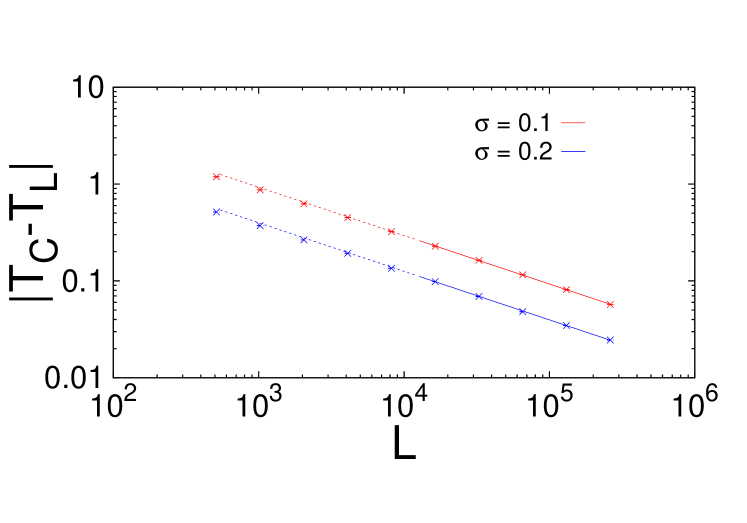
to the data, initially using , and the shift exponent as free parameters. To accommodate the presence of scaling corrections, which we do not include here explicitly, we successively removed system sizes from the small- end until satisfactory fit qualities were achieved. This resulted in system sizes being included in the fit. The data for the pseudocritical points together with these fits are shown in Fig. 1. The resulting parameters are with for , and with for , respectively. As is clearly seen, the estimates of the shift exponent are fully compatible with the -FSS prediction (4.5), , but not the conventional FSS result of . Having established confidence in the value of , in a second step we repeated the fits of the form (6.2) while fixing , resulting in the more precise estimates () and (). We employ these values for the scaling analysis at criticality. The results are summarized in Table 1. We note that our estimates of the transition temperatures are in complete agreement with those reported in Ref. [29].
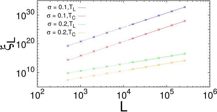
We now turn to the scaling of the correlation length as estimated from the second-moment form (5.5). Figure 2 summarizes our results for the correlation length for and . For the critical point and the data at the pseudocritical points defined from the susceptibility, we fit the functional form (1.1) to the data for the size range . The fits deliver () and () for and () and () for . This is in clear agreement with the relation (1.2) with , and inconsistent with the conventional expectation .
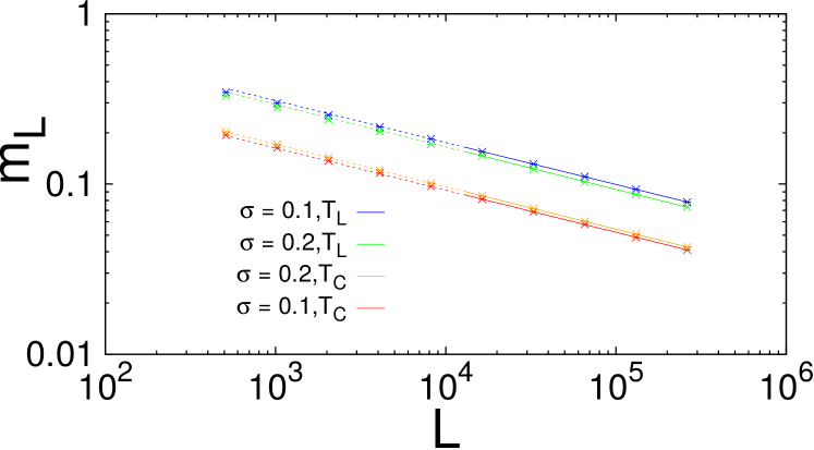
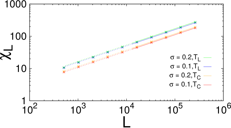
Our simulation results for the finite-size scaling of the magnetisation and susceptibility are depicted in Figs. 3 and 4, respectively. For the magnetisation, we fit the power-law (4.3) to the data at the critical point and for . We thus arrive at estimates for and for , respectively. Working at the maxima of the susceptibility, on the other hand, we find for and for . With and from Eqs. (2.4) and (2.5), respectively, these support over the alternative . For the susceptibility, when , we estimate the slope as at the critical point and at the pseudocritical point. The equivalent results for are and , respectively. Again, and from Eqs. (2.4) and (2.5), these support .
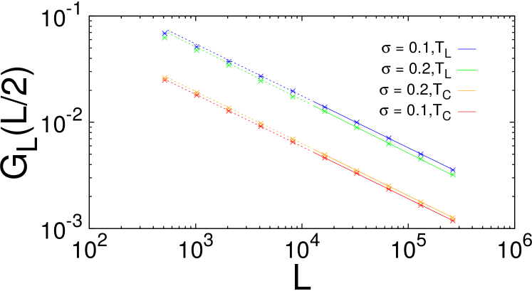
Finally we address the decay of the correlation function at the critical and pseudocritical points. In Fig. 5, the correlation function at is plotted against at both temperatures for and . The conventional expectation comes from Eq. (1.3) and gives in our case (). The -FSS prediction comes from Eq. (4.6) and is , independent of . The measured exponents, again restricting fits to the range , are at the critical point and at the pseudocritical point for . The corresponding measurements for are and , respectively. Thus the -FSS prediction is supported.
7 Discussion
The behaviour of the Ising model with long-range interactions remains a focus of investigation in the study of fundamental properties of critical phenomena. Here we examined the model in circumstances where the interaction range is sufficiently long for the model, although defined on a periodic chain, to be above its upper critical dimension. We have performed an extensive finite-size scaling study at both the infinite-volume critical points and the finite-volume pseudocritical points and confirmed that global quantities such as the magnetization and the susceptibility scale with a modified version of finite-size scaling. The origin of this modification to standard FSS is the occurrence of dangerous irrelevant variables above . Recent theoretical developments indicate that, contrary to long-standing belief, dangerous irrelevant variables also alter the behaviour of the correlation length and correlation function in high dimensions [1, 2, 9]. Here, we use extensive cluster-update Monte Carlo simulations of the model close to criticality to investigate finite-size scaling in this model and find that indeed this alteration does occur for interaction ranges corresponding to the system being above its upper critical dimension. In particular, the algebraic scaling law is supported, wherein . Turning to the decay of the correlation function on a finite-size lattice, the FSS theory presented in [9] shows that, above , this is not captured by the anomalous dimension derived from Landau or mean field theory. We have demonstrated this to be the case also in the one-dimensional model with sufficiently long range and instead it is described by a new exponent .
Acknowledgements:
This research was supported by the Leipzig-Lorraine-Lviv-Coventry Doctoral College of the German-French University for the Statistical Physics of Complex Systems and by a Marie Curie (RAVEN, MC-IIF-300206) and IRSES grants (SPIDER, PIRSES-GA-2011-295302 and DIONICOS, PIRSES-GA-2013-612707) within the 7th EU Framework Programme. M.W. acknowledges funding in the Emmy Noether programme of the DFG under contract No. WE-4425/1.
References
- [1] B. Berche, R. Kenna and J.-C. Walter, Nucl. Phys. B 865 (2012) 115-132.
- [2] R. Kenna and B. Berche, Condens. Matter Phys. 16 (2013) 23601.
- [3] K. Binder, M. Nauenberg, V. Privman, and A.P. Young, Phys. Rev. B 31 (1985) 1498-1502.
- [4] E. Brézin, J. Physique 43 (1982) 15-22.
- [5] N. Aktekin, Ş Erkoç and M. Kalay, Int. J. Mod. Phys. C 10 (1999) 1237-1245; N. Aktekin and Ş. Erkoç, Physica A 284 (2000) 206-214; Z. Merdan, A. Duran, D. Atille, G. Mülazimoğlu and A. Günen, Physica A 366 (2006) 265-272.
- [6] J.L. Jones and A.P. Young, Phys. Rev. B 71 (2005) 174438.
- [7] H.G. Katzgraber, D. Larson, and A.P. Young. Phys. Rev. Lett. 102 (2009) 177205; D. Larson, H.G. Katzgraber, M.A.Moore and A.P. Young Phys. Rev. B 81 (2010) 064415.
- [8] F. Beyer, M. Weigel, and M.A. Moore. Phys. Rev. B 86 (2012) 014431.
- [9] R. Kenna ad B. Berche, EPL 105 (2014) 26005.
- [10] M.E. Fisher, J. Math. Phys. 5 (1964) 944-962.
- [11] M.N. Barber, Finite-size scaling in Phase transitions and critical phenomena Vol. 8, edited by C. Domb and J.L. Lebowitz (Academic Press, New York, 1983), pp. 145-266.
- [12] M.E. Fisher, S.K. Ma, and B.G. Nickel. Phys. Rev. Lett. 29(14) (1972) 917-920.
- [13] M. C. Angelini, G. Parisi and F. Ricci-Tersenghi, Phys. Rev. E 89 (2014) 062120.
- [14] J. Sak. Phys. Rev. B 8(1) (1973) 281-285.
- [15] J. Honkonen and M.Y. Nalimov. J. Phys. A 22(6) (1989) 751-763.
- [16] J. Fröhlich and T. Spencer. Commun. Math. Phys. 84(1) (1982) 87-101.
- [17] M. Picco, arXiv:1207.1018.
- [18] T. Blanchard, M. Picco and M.A. Rajapbour, EPL 101 (2013) 56003.
- [19] E. Brezin, G. Parisi and F. Ricci-Tersenghi, J. Stat. Phys. 157(4-5) (2014) 855-868.
- [20] M. Abramowitz and I.A. Stegun. Handbook of Mathematical Functions: with Formulas, Graphs, and Mathematical Tables (Dover Books on Mathematics). Dover Publications, 1st edition, June 1965.
- [21] M.E. Fisher, Rev. Mod. Phys. 70 (1998) 653-681.
- [22] F.J. Wegner, Phys. Rev. B 5 (1972) 4529-4536.
- [23] M.E. Fisher, in Lecture notes in physics 186, critical phenomena, ed F.J.W. Hahne, (Springer, Berlin, 1983) pp. 1-139.
- [24] K. Binder, model, Z. Phys. B 61 (1985) 13-23.
- [25] I.G. Brankov, D.M. Danchev and N.S. Tonchev, Theory of critical phenomena in finite-size systems: scaling and quantum effects, (World Scientific, Singapore, 2000).
- [26] E. Luijten and H.W.J. Blöte, Phys. Rev. B 56 (1997) 8945-8958.
- [27] K. Binder and D.P. Landau. A Guide to Monte Carlo Simulations in Statistical Physics. Cambridge University Press, Cambridge, 3rd edition, 2009.
- [28] R.H. Swendsen and J.S. Wang. Phys. Rev. Lett. 58 (1987) 86-88.
- [29] E. Luijten, Interaction range, universality and the upper critical dimension, (Delft University Press, Delft 1997).
- [30] E. Luijten and H.W. Bl öte. Int. J. Mod. Phys. C 06(03) (1995) 359-370.
- [31] K. Fukui and S. Todo. J. Comp. Phys. 228(7) (2009) 2629-2642.
- [32] C.M. Fortuin and P.W. Kasteleyn. Physica, 57(4) (1972) 536-564.
- [33] D.E. Knuth. The Art of Computer Programming, Volume 2: Seminu- merical Algorithms. Addison-Wesley, Upper Saddle River, NJ, 3rd edition, 1997.
- [34] M.E.J. Newman and R. M. Ziff. Phys. Rev. E 64 (2001) 016706.
- [35] W. Janke. Monte carlo simulations of spin systems. In K. H. Hoffmann and M. Schreiber, editors, Computational Physics, pages 10-43. Springer, Berlin, 1996.
- [36] M. Suzuki. Critical exponents for Long-Range interactions. i. Prog. Theor. Phys. 49(2) (1973) 424-441.
- [37] H.G. Ballesteros, A. Cruz, L.A. Fernández, V. Martín-Mayor, J. Pech, J.J. Ruiz-Lorenzo, A. Tarancón, P. Téllez, C.L. Ullod, and C. Ungil. Phys. Rev. B, 62 (2000) 14237.