braidlab: a software package
for braids and loops

Abstract

braidlab is a Matlab package for analyzing data using braids. It was designed to be fast, so it can be used on relatively large problems. It uses the object-oriented features of Matlab to provide a class for braids on punctured disks and a class for equivalence classes of simple closed loops. The growth of loops under iterated action by braids is used to compute the topological entropy of braids, as well as for determining the equality of braids. This guide is a survey of the main capabilities of braidlab, with many examples; the help messages of the various commands provide more details. Some of the examples contain novel observations, such as the existence of cycles of the linear effective action for arbitrary braids.

1 What are braids?

1.1 A brief introduction to the braid group

Braids are collections of strings anchored between two planes,

Figure 1: (a) A geometric braid with five strings. (b) The corresponding braid diagram.

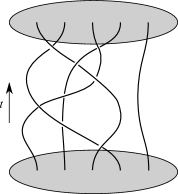
as in Fig. 1. More precisely this is called a geometric braid. In this case we can think of the vertical axis as ‘time’ and the horizontal axes as ‘space.’ The strings cannot occupy the same point in space at the same time, and they can’t reverse direction (i.e., they can’t go back in time). We consider two braids to be equal if their strings can be deformed into each other, with no string crossing another. The points on the bottom plane where the strings emanate in Fig. 1 are the same as the points on the top plane. In that sense braids naturally represent periodic orbits of two-dimensional dynamical systems. When slicing the braid horizontally at any given time we get a collection of points in the 2D plane, corresponding to the strings. We call these points punctures or particles.

In fact the set of all braids with a given number of strings, and the same anchorpoints, form a group. The group multiplication law is simply to lay one braid after another; it is easy to see that this is associative. The identity braid consists of straight strings that are unentangled with each other. The inverse of a braid is obtained by reversing time. (See the book by Birman for more details.)

A convenient way to represent a braid is to deform it as in Fig, 1. Here the geometric braid is combed such that only one crossing occurs at a time, and each crossing fits in a time interval of the same length. Such a picture is called a braid diagram. The operation of the $i$th string (counted from left to right) being exchanged with the $(i+1)$th string, such that the left string passes over the right, is called a generator of the braid group, as is denoted $\sigma_{i}$. Any element of the braid group on $n$ strings can be written as a product of the generators $\{\sigma_{1},\ldots,\sigma_{n-1}\}$ and their inverses. Thus, the braid in Fig. 1 can be written

$$\sigma_{3}\,\sigma_{2}^{-1}\sigma_{1}^{-1}\,\sigma_{2}\sigma_{3}^{-1}\sigma_{2}\sigma_{1}^{-1}\sigma_{3}^{-1}\,,$$ (1)

where we read the generators from left to right, and from bottom to top in Fig. 1. A braid written in terms of generators as in (1) is called an algebraic braid.

Figure 2: (a) Generators that don’t share a string commute. (b) The braid relation.

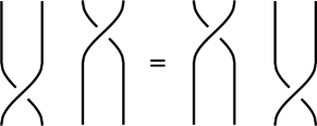
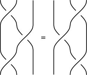
The generators obey some special rules, called relations, by virtue of arising from geometrical braids. The relations are

$$\sigma_{j}\sigma_{k}=\sigma_{k}\sigma_{j},\quad\lvert j-k\rvert>1;\qquad\sigma_{j}\sigma_{k}\sigma_{j}=\sigma_{k}\sigma_{j}\sigma_{k},\quad\lvert j-k\rvert=1.$$ (2)

The first type of relation, depicted in Fig. 2, says that generators commute if they don’t share a string. The second type, often called the braid relation, reflects the equality of the two braids shown in Fig. 2. While it’s obvious from Fig. 2 that the relations (2) are satisfied, it is far less obvious that those are the only relations that hold, as proved by Artin (1947). Hence, the relations (2) fully characterize the braid group for $n$ strings, denoted $B_{n}$.

1.2 Constructing a braid from orbit data

Figure 3: (a) The two types of generators that occur when particles exchange positions. (b) A particle exchanging position twice in a row with another leads to the generators $\sigma_{i}$ followed by $\sigma_{i}^{-1}$, which cancel each other. [After Thiffeault (2005).]

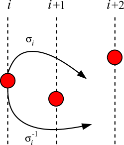
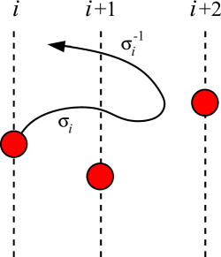
So far we have regarded braids as geometrical objects, and showed how to turn them into algebraic objects by writing them in terms of generators. But in practice how do we create braids from particle orbits? That is, if we have two-dimensional continuous trajectory data arising from some dynamical system, how do we turn this data into a braid?

The technique to do this was described in Thiffeault (2005). We define an arbitrary line in the 2D plane, called the projection line, and look at the order of the particles projected along that line. We label each particle according to its order when projected on this line. In Fig. 3, for example, we see three particles labeled $i$, $i+1$, $i+2$, where the projection line is the horizontal.

A crossing occurs whenever any two particles exchange position (only adjacent particles can exchange position at a given time, since the trajectories are continuous). For particle $i$ exchanging position with particle $i+1$, we assign a generator $\sigma_{i}$ to the crossing if the particle on the left passes above the one on the right, and $\sigma_{i}^{-1}$ if it passes below (Fig. 3). As we watch the trajectories unfold, we construct an algebraic braid as a sequence of generators, with each generator corresponding to a crossing, and their order determined by when each crossing occurs. Note that when two particles exchange position along the crossing line twice as in Fig. 3, without exchanging positions vertically, then the two crossings yield the generators $\sigma_{i}$ followed by $\sigma_{i}^{-1}$, which cancel.

The outcome of this procedure is not a true geometric braid, since the particles do not necessarily end up in the same positions as they started. (If the particles are part of a periodic orbit, then we do obtain a geometric braid.) We do however obtain an algebraic braid, and as long as we are careful to take long enough trajectories the fact that the geometric braid does not close will not be too consequential.

2 A tour of braidlab

You will need access to a recent version of Matlab to use braidlab. See Appendix A for instructions on how to install braidlab on your machine.

2.1 The braid class

2.1.1 Constructor and elementary operations

braidlab defines a number of classes, most importantly braid and loop. The braid $\sigma_{1}\sigma_{2}^{-1}$ is constructed with

⬇

>> a = braid([1 -2]) % defaults to 3 strings

a = < 1 -2 >

which defaults to the minimum required strings, $3$. The same braid on $4$ strings is constructed with

⬇

> a4 = braid([1 -2],4) % force 4 strings

a4 = < 1 -2 >

Two braids can be multiplied:

⬇

>> a = braid([1 -2]); b = braid([1 2]);

>> a*b, b*a

ans = < 1 -2 1 2 >

ans = < 1 2 1 -2 >

Powers can also be taken, including the inverse:

⬇

>> a^5, inv(a), a*a^-1

ans = < 1 -2 1 -2 1 -2 1 -2 1 -2 >

ans = < 2 -1 >

ans = < 1 -2 2 -1 >

Note that this last expression is the identity braid, but is not simplified. The method compact attempts to simplify the braid:

⬇

>> compact(a*a^-1)

ans = < e >

The method compact is based on the heuristic algorithm of Bangert et al. (2002), since finding the braid of minimum length in the standard generators is in general difficult (Paterson & Razborov, 1991). Hence, there is no guarantee that in general compact will find the identity braid, even though it does so here. To really test if a braid is the identity (trivial braid), use the method istrivial:

⬇

>> istrivial(a*a^-1)

ans = 1

The number of strings is

⬇

>> a.n

ans = 3

Note that

⬇

>> help braid

describes the class braid. To get more information on the braid constructor, invoke

⬇

>> help braid.braid

which refers to the method braid within the class braid. (Use methods(braid) to list all the methods in the class.) There are other ways to construct a braid, such as using random generators, here a braid with $5$ strings and $10$ random generators:

⬇

>> braid(’Random’,5,10)

ans = < 1 4 -4 2 4 -1 -2 4 4 4 >

The constructor can also build some standard braids:

⬇

>> braid(’HalfTwist’,5)

ans = < 4 3 2 1 4 3 2 4 3 4 >

>> braid(’8_21’) % braid for 8-crossing knot #21

ans = < 4 3 2 1 4 3 2 4 3 4 >

In Section 2.2 we will show how to construct a braid from a trajectory data set.

The braid class handles equality of braids:

⬇

>> a = braid([1 -2]); b = braid([1 -2 2 1 2 -1 -2 -1]);

>> a == b

ans = 1

These are the same braid, even though they appear different from their generator sequence (Birman, 1975). Equality is determined efficiently by acting on loop coordinates (Dynnikov, 2002), as described by Dehornoy (2008). See Sections 2.3–2.4 for more details. If for some reason lexicographic (generator-per-generator) equality of braids is needed, use the method lexeq(b1,b2).

We can extract a subbraid by choosing specific strings: for example, if we take the $4$-string braid $\sigma_{1}\sigma_{2}\sigma_{3}^{-1}$ and discard the third string, we obtain $\sigma_{1}\sigma_{2}^{-1}$:

⬇

>> a = braid([1 2 -3]);

>> subbraid(a,[1 2 4]) % subbraid using strings 1,2,4

ans = < 1 -2 >

The opposite of subbraid is the tensor product, the larger braid obtained by laying two braids side-by-side (Kassel & Turaev, 2008):

⬇

>> a = braid([1 2 -3]); b = braid([1 -2]);

>> tensor(a,b)

ans = < 1 2 -3 5 -6 >

Here, the tensor product of a 4-braid and a 3-braid has 7 strings. The generators $\sigma_{1}\sigma_{2}^{-1}$ of b became $\sigma_{5}\sigma_{6}^{-1}$ after re-indexing so they appear to the right of a.

2.1.2 Topological entropy and complexity

There are a few methods that exploit the connection between braids and homeomorphisms of the punctured disk. Braids label isotopy classes of homeomorphisms, so we can assign a topological entropy to a braid:

⬇

>> entropy(braid([1 2 -3]))

ans = 0.8314

The entropy is computed by iterated action on a loop (Moussafir, 2006). This can fail if the braid is finite-order or has very low entropy:

⬇

>> entropy(braid([1 2]))

Warning: Failed to converge to requested tolerance; braid is likely finite-order or has low entropy. Returning zero entropy.

ans = 0

To force the entropy to be computed using the Bestvina–Handel train track algorithm (Bestvina & Handel, 1995), we add an optional ’Method’ parameter:

⬇

>> entropy(braid([1 2]),’Method’,’train’)

ans = 0

Note that for large braids the Bestvina–Handel algorithm is impractical.

The topological entropy is a measure of braid complexity that relies on iterating the braid. It gives the maximum growth rate of a ‘rubber band’ anchored on the braid, as the rubber band slides up many repeated copies of the braid. For finite-order braids, this will converge to zero. The geometric complexity of a braid (Dynnikov & Wiest, 2007), is defined in terms of the $\log_{2}$ of the number of intersections of a set of curves with the real axis, after one application of the braid:

⬇

>> complexity(braid([1 -2]))

ans = 2

>> complexity(braid([1 2]))

ans = 1.5850

See Section 2.3 or ‘help braid.complexity’ for details on how the geometric complexity is computed.

2.1.3 Train track map and transition matrix

The Bestvina–Handel train track algorithm (Bestvina & Handel, 1995) can be used to determine the Thurston–Nielsen type of the braid as well as the train track map and its transition matrix (Fathi et al., 1979; Thurston, 1988; Casson & Bleiler, 1988; Boyland, 1994):

⬇

>> train(braid([1 2 -3]))

ans = struct with fields:

braid: [1x1 braidlab.braid]

tntype: ’pseudo-Anosov’

entropy: 0.8314

transmat: [4x4 double]

ttmap: {8x1 cell}

>> train(braid([1 2]))

ans = struct with fields:

braid: [1x1 braidlab.braid]

tntype: ’finite-order’

entropy: 0

transmat: [3x3 double]

ttmap: {6x1 cell}

>> train(braid([1 2],4)) % reducing curve around 1,2,3

ans = struct with fields:

braid: [1x1 braidlab.braid]

tntype: ’reducible’

entropy: 0

transmat: [3x3 double]

ttmap: {7x1 cell}

braidlab uses Toby Hall’s implementation of the Bestvina–Handel algorithm (Hall, 2012).

The train track map can be displayed in a human-readable format using the command ttmap:

⬇

>> tt = train(braid([1 2 -3]));

>> ttmap(tt)

1 -> 4

2 -> 1

3 -> 2

4 -> 3

a -> D

b -> d a -3 b -4 B

c -> B 3 A

d -> c

Here peripheral (infinitesimal) edges are denoted by numbers and main edges by letters. Inverse main edges are denoted by capital letters. The display of infinitesimal edges can be suppressed:

⬇

>> ttmap(tt,’Peripheral’,false)

a -> D

b -> d a b B

c -> B A

d -> c

The transition matrix associated with the train track map does not contain the peripheral edges, since these do not affect the entropy:

⬇

>> tt.transmat

ans = 0 1 1 0

0 2 1 0

0 0 0 1

1 1 0 0

>> max(abs(eig(ans)))

ans = 2.2966

2.1.4 Representation and invariants

There are a few remaining methods in the braid class, which we describe briefly. The reduced Burau matrix representation (Burau, 1936; Birman, 1975) of a braid is obtained with the method burau:

⬇

>> burau(braid([1 -2]),-1)

ans = 1 -1

-1 2

where the last argument ($-1$) is the value of the parameter $t$ in the Laurent polynomials that appear in the entries of the Burau matrices. With access to Matlab’s wavelet toolbox, we can use actual Laurent polynomials as the entries:

⬇

>> B = burau(braid([1 -2]),laurpoly(1,1))

| - z^(+1) z^(+1) |

| |

B = | |

| |

| - 1 + 1 - z^(-1) |

but the matrix is now given as a cell array , each entry containing a laurpoly object:

⬇

>> B{2,2}

ans(z) = + 1 - z^(-1)

Instead of laurpoly objects, we can use Matlab’s symbolic toolbox:

⬇

>> B = burau(braid([1 -2]),sym(’t’))

B = [ -t, t]

[ -1, 1 - 1/t]

where now B is a matrix of sym objects:

⬇

>> B(2,2)

ans = 1 - 1/t

Another well-known homological representation of braid groups is the Lawrence–Krammer representation (Lawrence, 1990; Bigelow, 2001). It is given in terms of two parameters, usually denoted $t$ and $q$:

⬇

>> K = lk(braid([1 -2]),sym(’t’),sym(’q’))

K = [ -(q-1)^2/q - q*t*(q-1), -(q-1)/q, (q^2-q+1)/q^2]

[ -q^2*t, 0, 0]

[ -(q-1)/(q*t), -1/(q*t), (q-1)/(q^2*t)]

In this case there we cannot use laurpoly entries, since the representation involves Laurent polynomials in two symbols. For this reason, and because its size grows more rapidly with the number of strings (matrices of dimension $\tfrac{1}{2}n(n-1)$), the Lawrence–Krammer representation is very slow to compute for large braids.

The reduced Burau matrix of a braid can be used to compute the Alexander–Conway polynomial (or Alexander polynomial for short) of its closure. For instance, the trefoil knot is given by the closure of the braid $\sigma_{1}^{3}$ (Weisstein, 2013), which gives a Laurent polynomial

⬇

>> alexpoly(braid([1 1 1])) % can also use braid(’Trefoil’)

ans(z) = + z^(+2) - z^(+1) + 1

The figure-eight knot is the closure of $(\sigma_{1}\sigma_{2}^{-1})^{2}$:

⬇

>> alexpoly(braid([1 -2 1 -2])) % or braid(’Figure-8’)

ans(z) = - 1 + 3*z^(-1) - z^(-2)

This can be ‘centered’ so that it satisfies $p(z)=\pm p(1/z)$:

⬇

>> alexpoly(braid([1 -2 1 -2]),’Centered’)

ans(z) = - z^(+1) + 3 - z^(-1)

The centered Alexander polynomial is a knot invariant, so it can be used to determine when two knots are not the same. For knots, the centered polynomial is guaranteed to have integral powers. For links, such as the Hopf link consisting of two singly-linked loops, it might not:

⬇

>> alexpoly(braid([1 1]),’Centered’) % the Hopf link

Error using braidlab.braid/alexpoly

Polynomial with fractional powers. Remove ’Centered’ option or use the symbolic toolbox.

Fractional powers cannot be represented with a laurpoly object. In that case we can drop the Centered option, which yields the uncentered polynomial $1-z$. Alternatively, we can switch to using a variable from the symbolic toolbox:

⬇

>> alexpoly(braid([1 1]),sym(’x’),’Centered’)

ans = 1/x^(1/2) - x^(1/2)

which can represent fractional powers. This polynomial satisfies $p(x)=-p(1/x)$.

The method perm gives the permutation of strings corresponding to a braid:

⬇

>> perm(braid([1 2 -3]))

ans = 2 3 4 1

If the strings are unpermuted, then the braid is pure, which can also be tested with the method ispure.

Finally, the writhe of a braid is the sum of the powers of its generators. The writhe of $\sigma_{1}^{+1}\sigma_{2}^{+1}\sigma_{3}^{-1}$ is $+1+1-1=1$:

⬇

>> writhe(braid([1 2 -3]))

ans = 1

The writhe is a braid invariant.

2.1.5 The annbraid subclass

Figure 4: (a) Punctures in an annular domain, with two generators. The generator $\Sigma_{n}$ is unique to the annulus. (b) The punctures rearranged with the center of the annulus as an extra puncture on the right, showing how the generator $\Sigma_{n}$ can be deformed in terms of standard generators as in (3).

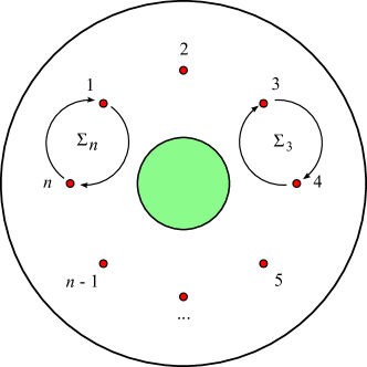
Often it is useful to consider braids in an annular domain, as in Fig. 4. It is convenient to rearrange the punctures as in Fig. 4, since the overall topology is unchanged. The center of the annulus becomes an extra puncture, but that extra puncture is fixed. For $n$ moving punctures, the braid group on the annulus has $n$ generators $\{\Sigma_{1},\ldots,\Sigma_{n}\}$, one more than for the standard braid group, owing to the fixed puncture. These are related to the standard generators by $\Sigma_{i}=\sigma_{i}$ for $1\leq i<n$, and

$$\Sigma_{n}=\sigma_{n}^{2}\sigma_{n-1}\cdots\sigma_{2}\,\sigma_{1}\,\sigma_{2}^{-1}\cdots\sigma_{n-1}^{-1}\sigma_{n}^{-2}\,.$$ (3)

This last generator effectively exchanges puncture $n$ with puncture $1$, exploiting the annular topology. These kinds of braids were considered in Boyland (1994); Finn et al. (2006); Finn & Thiffeault (2011).

braidlab supports annular braids with the subclass annbraid, derived from braid. The syntax for creating an annular braid is

⬇

>> b = annbraid([1 2 -3])

b = < 1 2 -3 >*

The asterisk indicates that this is an annular braid, which has an extra fixed puncture on the right (called the basepoint). Hence, the braid has $4$ punctures, as indicated by

⬇

>> b.n % total number of punctures, including the fixed one

ans = 4

but only $3$ punctures can move, as returned by nann, the number of annular punctures:

⬇

>> b.nann % number of moving punctures

ans = 3

Many of the methods work described for the braid class can be applied to annbraids. For instance,

⬇

>> entropy(braid([1 -2]))) % entropy of a normal braid

ans = 0.9624

>> entropy(annbraid([1 -2]))) % entropy of annular braid

ans = 1.7627

The annular braid has more entropy, since curves grow faster by getting entangled on the extra puncture (Finn & Thiffeault, 2011).

Figure 5: The output of plot(annbraid([1 -2])). The green strand represents the center of the annulus, as in Fig. 4. (See Section 6 for how to plot braids sideways.)

The annular braid is shown in Fig. 5.

2.2 Constructing a braid from data

2.2.1 An example

One of the main purposes of braidlab is to analyze two-dimensional trajectory data using braids. We can assign a braid to trajectory data by looking for crossings along a projection line (see Thiffeault (2005, 2010) and Section 2.2). The braid constructor allows us to do this easily.

The folder testsuite/testcases contains a dataset of trajectories, from laboratory data for granular media (Puckett et al., 2012). We load the data:

⬇

>> clear; load testdata

>> whos

Name Size Bytes Class Attributes

XY 9740x2x4 623360 double

ti 1x9740 77920 double

Here ti is the vector of times, and XY is a three-dimensional array: its first component specifies the timestep, its second specifies the $X$ or $Y$ coordinate, and its third specifies one of the $4$ particles. Figure 6 shows

Figure 6: (a) A dataset of four trajectories, (b) projected along the $X$ axis. (c) The compacted braid $\sigma_{2}^{-2}\sigma_{1}^{-1}\sigma_{2}^{-1}\sigma_{1}^{-5}\sigma_{3}\sigma_{1}^{-1}\sigma_{3}\sigma_{2}\sigma_{1}$ corresponding to the $X$ projection in (b). (d) The compacted braid $\sigma_{3}^{-4}\sigma_{1}\sigma_{3}^{-1}\sigma_{1}\sigma_{3}^{-3}$ corresponding to the $Y$ projection, with closure enforced. The braids in (c) and (d) are conjugate.

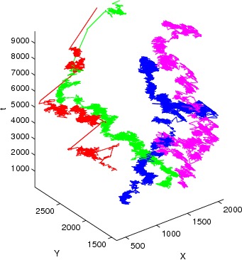
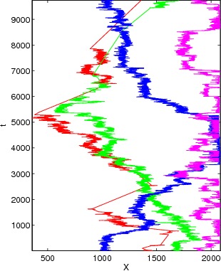
the $X$ and $Y$ coordinates of these four trajectories, with time plotted vertically. Figure 6 shows the same data, but projected along the $X$ direction. To construct a braid from this data, we simply execute

⬇

>> warning(’off’,’BRAIDLAB:braid:colorbraiding:notclosed’)

>> b = braid(XY);

>> b.length

ans = 894

This is a very long braid! (We’ve temporarily turned off a warning about the data not being closed; we’ll see what it’s about in Section 2.2.2.) But Figure 6 suggests that this is misleading: many of the crossings are ‘wiggles’ that cancel each other out. Indeed, if we attempt to shorten the braid:

⬇

>> b = compact(b)

b = < -2 -2 -1 -2 -1 -1 -1 -1 -1 3 -1 3 2 1 >

>> b.length

ans = 14

we find the number of generators (the length) has dropped to $14$! We can then plot this shortened braid as a braid diagram using plot(b) to produce Figure 6. The braid diagram allows us to see some topological information clearly, such as the fact that the second and third particles undergo a large number of twists around each other; we can check this by creating a subbraid with only those two strings:

⬇

>> subbraid(b,[2 3])

ans = < -1 -1 -1 -1 -1 -1 -1 -1 >

which shows that the winding number between these two strings is $-4$.

2.2.2 Changing the projection line and enforcing closure

The braid in the previous section was constructed from the data by assuming a projection along the $X$ axis (the default). We can choose a different projection by specifying an optional angle for the projection line; for instance, to project along the $Y$ axis we invoke

⬇

>> b = braid(XY,pi/2); % project onto Y axis

>> b.length

ans = 673

>> b.compact

ans = < -3 -3 -3 -3 1 -3 -3 -3 -3 >

In general, a change of projection line only changes the braid by conjugation (Boyland, 1994; Thiffeault, 2010). We can test for conjugacy:

⬇

>> bX = compact(braid(XY,0)); bY = compact(braid(XY,pi/2));

>> conjtest(bX,bY) % test for conjugacy of braids

ans = 0

The braids are not conjugate. This is because our trajectories do not form a ‘true’ braid: the final points do not correspond exactly with the initial points, as a set. This is the reason why we turned off a warning in Section 2.2.1: braidlab warns us when we’re trying to create a braid from data that doesn’t ‘join up.’ The class databraid described in Section 2.2.3 does not issue this warning, since it is meant for noisy real-world data.

If we truly want a rotationally-conjugate braid out of our data, we need to enforce a closure method:

⬇

>> XY = closure(XY); % close braid and avoid new crossings

>> bX = compact(braid(XY,0)), bY = compact(braid(XY,pi/2))

bX = < -2 -2 -1 -2 -1 -1 -1 -1 -1 3 -1 3 2 1 >

bY = < -3 -3 -3 -3 1 -3 1 -3 -3 -3 >

This default closure simply draws line segments from the final points to the initial points in such a way that no new crossings are created in the $X$ projection. Hence, the $X$-projected braid bX is unchanged by the closure, but here the $Y$-projected braid bY is longer by one generator (bY is plotted in Figure 6). This is enough to make the braids conjugate:

⬇

>> [~,c] = conjtest(bX,bY) % ~ means discard first return arg

c = < 3 2 >

where the optional second argument c is the conjugating braid, as we can verify:

⬇

>> bX == c*bY*c^-1

ans = 1

There are other ways to enforce closure of a braid (see help closure), in particular closure(XY,’MinDist’), which minimizes the total distance between the initial and final points.

Note that conjtest uses the library CBraid (Cha, 2011) to first convert the braids to Garside canonical form (Birman & Brendle, 2005), then to determine conjugacy. This is very inefficient, so is impractical for large braids.

2.2.3 The databraid subclass

In some instances when dealing with data it is important to know the crossing times, that is, the times at which two particles exchanged position along the projection line. A braid object does not keep this information, but there is an object that does: a databraid. Its constructor takes an optional vector of times as an argument, and it has a data member tcross that retains the crossing times. Using the same data XY from before, sampled at times ti, we have

⬇

>> b = databraid(XY,ti);

>> b.tcross(1:3)

ans = 870.9010

872.1758

887.0089

Storing crossing times enables us to truncate generators in a databraid by retaining only those with crossing times within a desired interval (see databraid.trunc). There are always exactly as many crossing times as generators in the braid.

Many operations that can be done to a braid also work on a databraid, with a few differences:

• compact works a bit differently. It is less effective than braid.compact since it must preserve the order of generators in order to maintain the ordering of the crossing times.

• Equality testing checks if two databraids are lexicographically equal (i.e., generator-by-generator) and that their crossing times all agree. This is very restrictive. To check if the underlying braids are equal, first convert the databraids to braids by using the method databraid.braid.

• Multiplication of two databraids is only defined if the crossing times of the first braid are all earlier than the second.

• Powers and inverses of databraids are not defined, since this would break the time-ordering of crossings.

• The entropy of a databraid is an ambiguously defined concept. While entropy of certain braids can be computed non-iteratively, e.g., in Hall & Yurttaş (2009), in general it is only estimated by an iterative process. Iterations rely on taking powers of the braid, which is not defined for databraids. The functions entropy and complexity can still be used by converting databraid objects to braid objects; however, this should be avoided in favor of the appropriate concept for databraids, the Finite Time Braiding Exponent (FTBE) (Thiffeault, 2005; Budišić & Thiffeault, 2015). A databraid $b_{T}$ recorded over a time interval of length $T$ has an FTBE defined by

  $$\operatorname{FTBE}(b_{T})=\frac{1}{T}\,\log\frac{\lvert b_{T}\,\ell\rvert}{\lvert\ell\rvert},$$ (4)

  where $\ell$ is a loop given by the generating set for the fundamental group of the disk with $n$ punctures (see Section 2.4), and $b_{T}\ell$ is that loop transformed by a single application of the braid. Here $\lvert\cdot\rvert$ is a measure of the length of the loop. Unless specified otherwise, braidlab calculates $T$ as the time elapsed between the first and last crossing in the braid. This duration could be much smaller than the length of trajectories analyzed, e.g., when no crossings occur near the beginning or the end of trajectories. To set the custom value of $T$ and other options, see documentation of the method databraid.ftbe.

2.3 The loop class

2.3.1 Loop coordinates

A simple closed loop on a disk with $5$ punctures is shown in Figure 7.

Figure 7: (a) A simple close loop in a disk with $n=5$ punctures. (b) Definition of intersection numbers $\mu_{i}$ and $\nu_{i}$. [From Thiffeault (2010).]

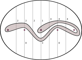
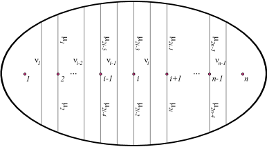
We consider equivalence classes of such loops under homotopies relative to the punctures. In particular, the loops are essential, meaning that they are not null-homotopic or homotopic to the boundary or a puncture. The intersection numbers are also shown in Figure 7: these count the minimum number of intersections of an equivalence class of loops with the fixed vertical lines shown. For $n$ punctures, we define the intersection numbers $\mu_{i}$ and $\nu_{i}$ in Figure 7.

Any given loop will lead to a unique set of intersection numbers, but a general collection of intersection numbers do not typically correspond to a loop. It is therefore more convenient to define

$$a_{i}=\tfrac{1}{2}\left(\mu_{2i}-\mu_{2i-1}\right),\qquad b_{i}=\tfrac{1}{2}\left(\nu_{i}-\nu_{i+1}\right),\qquad i=1,\ldots,n-2.$$ (5)

We then combine these in a vector of length $(2n-4)$,

$$\bm{u}=(a_{1},\ldots,a_{n-2},b_{1},\ldots,b_{n-2}),$$ (6)

which gives the loop coordinates (or Dynnikov coordinates) for the loop. (Some authors such as Dehornoy (2008) give the coordinates as $(a_{1},b_{1},\ldots,a_{n-2},b_{n-2})$.) There is now a bijection between $\mathbb{Z}^{2n-4}$ and essential simple closed loops (Dynnikov, 2002; Moussafir, 2006; Hall & Yurttaş, 2009; Thiffeault, 2010). Actually, multiloops: loop coordinates can describe unions of disjoint loops (see Section 2.4).

Let’s create the loop in Figure 7 as a loop object:

⬇

>> l = loop([-1 1 -2 0 -1 0])

l = (( -1 1 -2 0 -1 0 ))

Figure 8 shows the output of the plot(l) command. We can convert from loop coordinates to intersection numbers with

⬇

>> intersec(l)

ans = 2 0 1 3 4 0 2 2 4 4 % [mu1 … mu6 nu1 … nu4]

which returns $\mu_{1}\dots\mu_{2n-4}$ followed by $\nu_{1}\dots\mu_{n-1}$, as defined in Figure 7.

We can also extract the loop coordinates from a loop object using the methods a, b, and ab:

⬇

>> l = loop ([-1 1 -2 0 -1 0]);

>> l.a

ans = -1 1 -2

>> l.b

ans = 0 -1 0

>> [a,b] = l.ab

a = -1 1 -2

b = 0 -1 0

As for braids, l.n returns the number of punctures (or strings).

2.3.2 Acting on loops with braids

Now we can act on this loop with braids. For example, we define the braid b to be $\sigma_{1}^{-1}$ with $5$ strings, corresponding to the $5$ punctures, and then act on the loop l by using the multiplication operator:

Figure 8: (a) The loop ((-1 1 -2 0 -1 0)). (b) The braid generator $\sigma_{1}^{-1}$ applied to the loop in (a).

⬇

>> b = braid([-1],5); % one generator with 5 strings

>> b*l % act on a loop with a braid

ans = (( -1 1 -2 1 -1 0 ))

Figure 8 shows plot(b*l). The first and second punctures were interchanged counterclockwise (the action of $\sigma_{1}^{-1}$), dragging the loop along.

The minimum length of an equivalence class of loops is determined by assuming the punctures are one unit of length apart and have zero size. After pulling tight the loop on the punctures, it is then made up of unit-length segments. The minimum length is thus an integer. For the loop in Figure 8,

⬇

>> minlength(l)

ans = 12

Another useful measure of a loop’s complexity is its minimum intersection number with the real axis (Moussafir, 2006; Hall & Yurttaş, 2009; Thiffeault, 2010), which for this loop is the same as its minimum length:

⬇

>> intaxis(l)

ans = 12

The intaxis method is used to measure a braid’s geometric complexity, as defined by Dynnikov & Wiest (2007).

Sometimes we wish to study a large set of different loops. The loop constructor vectorizes:

⬇

>> ll = loop([-1 1 -2 0; 1 -2 3 4])

ll = (( -1 1 -2 0 ))

(( 1 -2 3 4 ))

We can then, for instance, compute the length of every loop:

⬇

>> minlength(ll)

ans = 14

34

or even act on all the loops with the same braid:

⬇

>> b = braid([1 -2]);

>> b*ll

ans = (( 2 1 -2 1 ))

(( 5 -2 -3 11 ))

Some commands, such as plot, do not vectorize. Different loops can then be accessed by indexing, such as plot(ll(2)).

The entropy method of the braid class (Section 2.1) computes the topological entropy of a braid by repeatedly acting on a loop, and monitoring the growth rate of the loop. For example, let us compare the entropy obtained by acting $100$ times on an initial loop, compared with the entropy method:

⬇

>> b = braid([1 2 3 -4]);

% apply braid 100 times to l, then compute growth of length

>> log(minlength(b^100*l)/minlength(l)) / 100

ans = 0.7637

>> entropy(b)

ans = 0.7672

The entropy value returned by entropy(b) is more precise, since that method monitors convergence and adjusts the number of iterations accordingly.

2.4 Loop coordinates for a braid

The command loop(n,’BasePoint’) returns a canonical set of loops for $n$ punctures:

⬇

>> l = loop(5,’BP’) % ’BP’ is short for ’BasePoint’

ans = (( 0 0 0 0 -1 -1 -1 -1 ))*

This multiloop is depicted in Figure 9, with basepoint puncture shown in green. The * indicates that this loop has a basepoint. Note that the multiloop returned by loop(5,’BP’) actually has 6 punctures! The rightmost puncture is meant to represent the boundary of a disk, or a base point for the fundamental group on a sphere with $n$ punctures. The loops form a (nonoriented) generating set for the fundamental group of the disk with $n$ punctures. The extra puncture thus plays no role dynamically, and l.n returns 5. If you want the true total number of punctures, including the base point, use l.totaln.

The canonical set of loops allows us to define loop coordinates for a braid, which is a unique normal form.

Figure 9: (a) The multiloop created by loop(5,’BP’), with basepoint puncture in green. (b) The multiloop b*loop(5,’BP’), where b is the braid $\sigma_{1}\sigma_{2}\sigma_{3}\sigma_{4}^{-1}$.

The canonical loop coordinates for braids exploit the fact that two braids are equal if and only if they act the same way on the fundamental group of the disk (Dehornoy, 2008). Hence, if we take a braid and act on loop(5,’BP’),

⬇

>> b = braid([1 2 3 -4]);

>> b*loop(5,’BP’)

ans = (( 0 0 3 -1 -1 -1 -4 3 ))*

then the set of numbers (( 0 0 3 -1 -1 -1 -4 3 ))* can be thought of as uniquely characterizing the braid. It is this property that is used to rapidly determine equality of braids. (The loop b*loop(5,’BP’) is plotted in Figure 9.) The same loop coordinates for the braid can be obtained without creating an intermediate loop with

⬇

>> loopcoords(b)

ans = (( 0 0 3 -1 -1 -1 -4 3 ))*

3 The effective linear action and its cycles

3.1 Effective linear action

In Section 2.3.2 we introduced the action of a braid $\gamma$ on a loop $\bm{u}$. Here $\bm{u}=(a_{1},\ldots,a_{n-2},b_{1},\ldots,b_{n-2})$ is a vector of coordinates for the loop, defined in Section 2.3.1. We write $\bm{u}^{\prime}=\gamma\cdot\bm{u}$ for the new, updated coordinates after the action. These updated coordinates are given by composing the action of individual generators.

For $1<i<n-1$, we can express the update rules for the braid group generator $\sigma_{i}$ acting on $\bm{u}$ as

$$a^{\prime}_{i-1} =a_{i-1}-b_{i-1}^{+}-\left(b_{i}^{+}+c_{i-1}\right)^{+}\,,$$ (7a)

$$b^{\prime}_{i-1} =b_{i}+c_{i-1}^{-}\,,$$ (7b)

$$a^{\prime}_{i} =a_{i}-b_{i}^{-}-\left(b_{i-1}^{-}-c_{i-1}\right)^{-}\,,$$ (7c)

$$b^{\prime}_{i} =b_{i-1}-c_{i-1}^{-}\,,$$ (7d)

where

$$c_{i-1}=a_{i-1}-a_{i}-b_{i}^{+}+b_{i-1}^{-}\,.$$ (8)

Coordinates not listed (i.e., $a_{k}$ and $b_{k}$ for $k\neq i$ or $i-1$) are unchanged. The superscripts ^+/- are defined as

$$f^{+}\mathrel{\raisebox{0.29707pt}{:}\!\!=}\max(f,0),\qquad f^{-}\mathrel{\raisebox{0.29707pt}{:}\!\!=}\min(f,0).$$ (9)

(See Thiffeault (2010) for the update rules for the generators $\sigma_{1}$, $\sigma_{n-1}$, and the inverse generators. The update rules are in several other papers but use different conventions.)

Notice that the action (7) is piecewise-linear in the loop coordinates: once the ^+/- operators are resolved, what is left is a linear operation on the vector $\bm{u}$. We can thus write

$$\bm{u}^{\prime}=M(\gamma,\bm{u})\cdot\bm{u},\qquad M(\gamma,\bm{u})\in\mathrm{SL}_{2n-4}(\mathbb{Z}),$$ (10)

where the dot now denotes the standard matrix product. Here $M(\gamma,\bm{u})$ is the effective linear action of the braid $\gamma$ on the loop $\bm{u}$.

Let’s show an example using braidlab. We take the braid $\sigma_{1}\sigma_{2}^{-1}$ and the loop with coordinates $a_{1}=0$, $b_{1}=-1$. The action is

⬇

>> b = braid([1 -2]); l = loop([0 -1]);

>> lp = b*l

lp = (( 1 -1 ))

The effective linear action can be obtained by requesting a second output argument from the result of *:

⬇

>> [lp,M] = b*l; full(M)

ans = 1 -1

0 1

Note that the effective linear action M is by default returned as a sparse matrix, which it often is when dealing with many strands. We use full to convert it back into a regular full matrix. We can then verify that the matrix product of M and the column vector of coordinates l.coords’ is the same as the action lp = b*l:

⬇

>> M*l.coords’

ans = 1

-1

>> lp.coords’

ans = 1

-1

The difference is that M may only be applied to this specific loop (or a loop that happens to share the same effective linear action).

A common thing to do is to find the effective linear action on the canonical set loop(b.n,’BP’) (see Section 2.4):

⬇

>> [~,M] = b*loop(b.n,’BP’); full(M)

ans = 0 0 -1 0

0 1 0 1

0 1 1 1

1 -1 -1 0

The canonical set assumes an extra puncture, so the matrix dimension is larger by $2$.

The effective linear action doesn’t seem to offer much at this point. Its real advantage will become apparent in Section 3.2, when we find that it can achieve periodic limit cycles.

3.2 Limit cycles of the effective linear action

The effective linear action has a very interesting behavior when a braid is iterated on some initial loop. Consider the following example:

⬇

>> b = braid([1 -2]); l = loop([1 1]);

>> [l,M] = b*l; l, full(M)

l = (( 3 -1 ))

M = 2 1

-1 0

Now repeat this last command:

⬇

>> [l,M] = b*l; l, full(M)

l = (( 7 -4 ))

M = 2 -1

-1 1

And again:

⬇

>> b = braid([1 -2]); l = loop([1 1]);

>> [l,M] = b*l; l, full(M)

l = (( 18 -11 ))

M = 2 -1

-1 1

The effective linear action M has not changed. In fact it has achieved a fixed point: running the same command again will change the loop, but the linear action will remain the same forever. braidlab can automate the iteration with the method cycle. Figure 10 shows the output of

Figure 10: The plot produced by cycle(b,’Plot’) for (a) b = braid([1 -2]); (b) b = braid([1 2 3]); (c) b = braid(’Psi’,11).

⬇

>> b = braid([1 -2]); M = cycle(b,’Plot’);

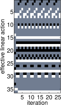
The member function cycle iterates the braid on an initial loop, taken to be the canonical set loop(b.n,’BP’). The vertical axis in Fig. 10 shows the elements of the effective linear action as a function of iterates of the braid. The matrix of the action is flattened into a vector of length $4^{2}$, where $4$ is the dimension the initial loop loop(b.n,’BP’). It is evident that the fixed point is reached rapidly, since the ‘stripes’ stop changing.

Such fixed points of the effective linear action are ubiquitous for braids corresponding to a pseudo-Anosov isotopy class, such as $\sigma_{1}\sigma_{2}^{-1}$. In general, instead of a fixed point we may find a limit cycle of some period. Yurttaş (2014) discussed these limit cycles for pseudo-Anosov braids: they occur when the unstable foliation falls on the boundary of the linear regions of the update rules. We can reproduce her example with the following:

⬇

>> b = braid([-1 -2 -3 4]);

>> M = b.cycle(loop(b.n),’Iter’)

M = [6x6 double] [6x6 double]

The option ’Iter’ tells cycle to compute an individual matrix for each iterate of the cycle, rather than the net product of all the matrices in the cycle. The output is a cell array of two $6$ by $6$ matrices, corresponding to the period-2 cycle:

⬇

>> full(M{1}), full(M{2})

ans = -1 1 0 0 0 0

0 0 0 1 1 0

0 0 2 -1 -1 1

0 0 0 0 1 0

-1 0 1 -1 -1 1

0 0 1 0 0 1

ans = 0 0 0 1 0 0

0 0 0 1 1 0

0 0 2 -1 -1 1

-1 1 0 -1 1 0

0 -1 1 0 -1 1

0 0 1 0 0 1

as given by Yurttaş (2014). Note that we use an initial loop for $n$ punctures (loop(b.n)) without base point, rather than the default, to reproduce her example exactly. For the pseudo-Anosov case, any initial loop will give the same matrices.

What is more surprising is that these limit cycles occur for finite-order braids as well. Figure 10 is produced by

⬇

>> b = braid([1 2 3]); [~,period] = cycle(b,’Plot’)

period = 4

Indeed, staring at the pattern in Fig. 10 it is easy to see that the effective action does achieve a limit cycle of period $4$. This braid is definitely not pseudo-Anosov: it is finite-order. However, we do not expect such limit cycles to be unique in the non-pseudo-Anosov case.

Pseudo-Anosov braids can achieve longer cycles, which braidlab can find: Figure 10 is the plot produced by

⬇

>> b = braid(’Psi’,11); [M,period] = cycle(b,’Plot’);

The period here is $5$, and the matrix $M$ is $20$ by $20$. The braid braid(’Psi’,11) is the braid $\psi_{11}$ in the notation of Venzke (2008). It is a pseudo-Anosov braid with low dilatation (Hironaka & Kin, 2006; Thiffeault & Finn, 2006), conjectured to be the lowest possible for $11$ strings. The braids $\psi_{n}$ are known to have to lowest dilatation for $n$ string for $n\leq 8$ (Lanneau & Thiffeault, 2011).

The largest eigenvalue of the matrix M gives us the dilatation of the braid, which in itself is not a real improvement over our earlier entropy iterative algorithm (Section 2.1.2). However, with the matrix in hand we can find the characteristic polynomial:

⬇

>> b = braid(’Psi’,7); [M,period] = cycle(b);

>> factor(poly2sym(charpoly(M))) % convert to symbolic form

ans = (x^2 + 1)*(x^3 - x^2 - 1)*(x^3 + x - 1)*(x - 1)^2*(x + 1)^2

Compare this to the known polynomial that gives the dilation:

⬇

>> factor(poly2sym(psiroots(7,’Poly’)))

ans = (x + 1)*(x^3 - x^2 - 1)*(x^3 + x - 1)

(The function psiroots returns the roots and characteristic polynomial of a $\psi$ braid; this is useful for testing purposes.) Note that the factor whose largest root is the dilatation, x^3 - x^2 - 1, appears in both polynomials. This is not always the case, though the dilatation has to be a root of both polynomials.

To our knowledge, the existence of these limit cycles has not been fully explained (except in the pseudo-Anosov case by Yurttaş (2014)). They seem to occur for any braid, regardless of its isotopy class. In that sense they could provide an alternative to the the Bestvina–Handel train track algorithm (Bestvina & Handel, 1995), which is used to compute the isotopy class of a braid.

4 An example: Taffy pullers

Taffy pullers are a class of devices designed to stretch and fold soft candy repeatedly (Finn & Thiffeault, 2011; Thiffeault, 2018). The goal is to aerate the taffy. Since many folds are required, the process has been mechanized using fixed and moving rods. The two most typical designs are shown in Figure 11: the one in

Figure 11: (a) Three-rod taffy puller. (b) Four-rod taffy puller.

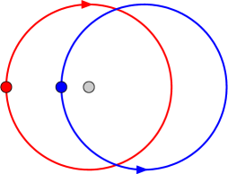
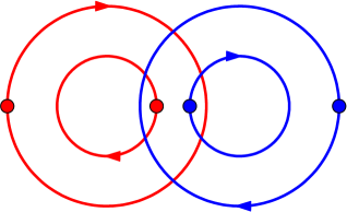
Figure 11 has a single fixed rod (gray) and two moving rods, each rotating on a different axis. The design in Figure 11 has four moving rods, sharing two axes of rotation. (There are several videos of taffy pullers on YouTube.)

Let’s use braidlab to analyze the rod motion. From the folder doc/examples, run the command

⬇

>> b = taffy(’3rods’)

b = < -2 1 1 -2 >

which also produces Figure 11. The Thurston–Nielsen type and topological entropy of this braid are

⬇

>> train(b)

ans = struct with fields:

braid: [1x1 braidlab.braid]

tntype: ’pseudo-Anosov’

entropy: 1.7627

transmat: [2x2 double]

ttmap: {5x1 cell}

One would expect a competent taffy puller to be pseudo-Anosov, as this one is. It implies that there is no ‘bad’ initial condition where a piece of taffy never gets stretched, or stretches slowly. A reducible or finite-order braid would indicate poor design. The entropy is a measure of the taffy puller’s effectiveness: it gives the rate of growth of curves anchored on the rods. Thus, the length of the taffy is multiplied (asymptotically) by $\mathrm{e}^{1.7627}\simeq 5.828$ for each full period of rod motion. Needless to say, this leads to extremely rapid growth, since after $10$ periods the taffy length has been multiplied by roughly $10^{7}$.

The design in Figure 11 can be plotted and analyzed with

⬇

>> b = taffy(’4rods’)

b = < 1 3 2 2 1 3 >

When we apply train to this braid we find the braid is pseudo-Anosov with exactly the same entropy as the 3-rod taffy puller, $1.7627$. There is thus no obvious advantage to using more rods in this case.

A simple modification of the 4-rod design in Figure 11 is shown in Figure 12.

Figure 12: (a) A six-rod taffy puller based on Figure 11, with two added fixed rods (gray). This is a poor design, since it leads to a reducible braid. (b) Same as (a), but with the same radius of motion for all the moving rods. The braid is in this case pseudo-Anosov, with larger entropy than the 4-rod design.

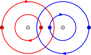
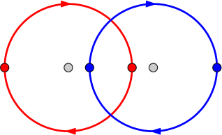
The only change is to extend the rotation axles into two extra fixed rods (shown in gray). The resulting braid is

⬇

>> b = taffy(’6rods-bad’)

b = < 2 1 2 4 5 4 3 3 2 1 2 4 5 4 >

with Thurston–Nielsen type

⬇

>> train(b)

ans = struct with fields:

braid: [1x1 braidlab.braid]

tntype: ’reducible’

entropy: 0

transmat: [5x5 double]

ttmap: {11x1 cell}

There are reducing curves in this design: simply wrap a loop around the left gray rod and the inner red rod, and it will rotate without stretching. To avoid this, we extend the radius of motion of the inner rods to equal that of the outer ones, and obtain the design shown in Figure 11. The corresponding braid is

⬇

>> b = taffy(’6rods’)

b = < 3 2 1 2 4 5 4 3 3 2 1 2 5 4 5 3 >

with Thurston–Nielsen type and entropy

⬇

>> [t,entr] = train(b)

ans = struct with fields:

braid: [1x1 braidlab.braid]

tntype: ’pseudo-Anosov’

entropy: 2.6339

transmat: [5x5 double]

ttmap: {11x1 cell}

The fixed rods have increased the entropy by $50\%$! This sounds like a fairly small change, but what it means is that this 6-rod design achieves growth of $10^{7}$ in about $6$ iterations rather than $10$. Alexander Flanagan constructed this six-rod device while an undergraduate student at the University of Wisconsin – Madison, but as far as we know this new design has not yet been used in commercial applications.

The symmetric design of the taffy pullers illustrates one pitfall when constructing braids. If we give an optional projection angle of $\pi/2$ to taffy:

⬇

>> taffy(’4rods’,pi/2)

Error using braidlab.braid/colorbraiding

Paths of particles 2 and 1 have a coincident projection.

Try changing the projection angle.

This corresponds to using the $y$ (vertical) axis to compute the braid, but as we can see from Figure 11 this is a bad choice, since all the rods are initially perfectly aligned along that axis. The braid obtained would depend sensitively on numerical roundoff when comparing the rod projections. Instead of attempting to construct the braid, braidlab returns an error and asks the user to modify the projection axis. A tiny change in the projection line is sufficient to break the symmetry:

⬇

>> taffy(’4rods’,pi/2 + .01)

ans = < -2 2 1 3 2 -3 -1 3 1 2 1 3 >

>> compact(ans)

ans = < 3 1 2 2 3 1 >

which is actually equal to the braid formed from projecting on the $x$ axis, though it need only be conjugate (see Section 2.2).

5 Side note: On filling-in punctures

Recall the command subbraid from Section 2.1. We took the $4$-string braid $\sigma_{1}\sigma_{2}\sigma_{3}^{-1}$ and discarded the third string, to obtain $\sigma_{1}\sigma_{2}^{-1}$:

⬇

>> a = braid([1 2 -3]);

>> b = subbraid(a,[1 2 4]) % discard string 3, keep 1,2,4

b = < 1 -2 >

Figure 13: Removing the third string from the braid (a) $\sigma_{1}\sigma_{2}\sigma_{3}^{-1}$ yields the braid (b) $\sigma_{1}\sigma_{2}^{-1}$.

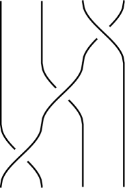
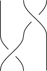
The braids a and b are shown in Fig. 13; their entropies are

⬇

>> a.entropy, b.entropy

ans = 0.8314

ans = 0.9624

Note that the entropy of the subbraid b is higher than the original braid. This is counter-intuitive: shouldn’t removing strings cause loops to shorten, therefore lowering their growth?

In some sense this must be true: consider the rod-stirring device shown in Fig. 14, where the rods move according the to braid $\sigma_{1}\sigma_{2}\sigma_{3}^{-1}$.

Figure 14: (a) The mixing protocol specified by the braid $\sigma_{1}\sigma_{2}\sigma_{3}^{-1}$ (Thiffeault et al., 2008). The inset shows how the rods are moved. (b) The pure braid $(\sigma_{1}\sigma_{2}\sigma_{3}^{-1})^{4}$. (c) The braid $(\sigma_{1}\sigma_{2}^{-1})^{2}\sigma_{1}\sigma_{2}$, obtained by removing the third string from (b).

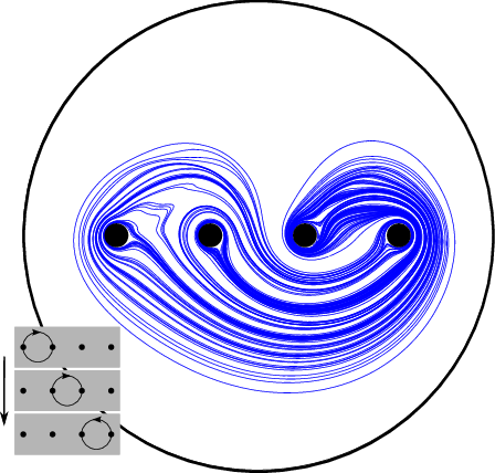
Removing the third string can be regarded as filling-in the third puncture (rod); clearly then the material line can be shortened, leading to a decrease in entropy.

The flaw in the argument is that even though we can remove any string, we cannot fill in a puncture that is permuted, since the resulting braid does not define a homeomorphism on the filled-in surface. To remedy this, let us take enough powers of the braid $\sigma_{1}\sigma_{2}\sigma_{3}^{-1}$ to ensure that the third puncture returns to its original position, using the method perm to find the permutation induced by the braid:

⬇

>> perm(a)

ans = 2 3 4 1

The permutation is cyclic (it can be constructed with exactly one cycle), so the fourth power should do it:

⬇

>> perm(a^4)

ans = 1 2 3 4

This is now a pure braid: all the strings return to their original position (Fig. 14). Now here’s the surprise: the subbraid obtained by removing the third string from a^4 is

⬇

>> b2 = subbraid(a^4,[1 2 4])

b2 = < 1 -2 1 -2 1 2 >

which is not b^4 (Fig. 14)! However, now there is no paradox in the entropies:

⬇

>> entropy(a^4), entropy(b2)

ans = 3.3258

Warning: Failed to converge to requested tolerance; braid is likely finite-order or has low entropy. Returning zero entropy.

ans = 0

braidlab has trouble computing the entropy because the braid b2 appears to be finite-order. Indeed, the braid b2 is conjugate to $\sigma_{1}^{2}$:

⬇

>> c = braid([2 -1],3);

>> compact(c*b2*c^-1)

ans = < 1 1 >

showing that its entropy is indeed zero.

The moral is: when filling-in punctures, make sure that the strings being removed are permuted only among themselves. For very long, random braids, we still expect that removing a string will decrease the entropy, since the string being removed will have returned to its initial position many times.

6 Setting global properties

Braids have been studied for a long time and by many communities, so several different conventions were bound to emerge. braidlab has some reasonable default conventions, but perhaps you’d be happier if it used your favorite one. Luckily, braidlab has you covered.

To see the properties available and their current values, use the prop command:

⬇

>> prop

ans = GenRotDir: 1

GenLoopActDir: ’lr’

GenPlotOverUnder: 1

BraidAbsTol: 1.0000e-10

BraidPlotDir: ’bt’

LoopCoordsBasePoint: ’right’

To set a property, use something like prop(’BraidPlotDir’,’lr’). This will plot braids from left-to-right from now on, as in Fig. 15.

Figure 15: plot(braid(’FullTwist’,5)) with the property ’BraidPlotDir’ set to ’lr’.

The default is ’bt’ for bottom-to-top. Other possible values are ’tb’ for top-to-bottom and ’rl’ for right-to-left. See help prop for more information on properties and allowed values.

Appendix A Installing braidlab

braidlab consists of Matlab files together with C and C++ auxiliary files, so-called MEX files. The MEX files are used to greatly speed up calculations. Many commands will work even if the MEX files are unavailable, but much more slowly. (A few commands won’t work at all.) However, MEX files need to be first compiled with Matlab’s mex compiler.

A.1 Precompiled packages

Some tar files of the precompiled latest released version are available at http://github.com/jeanluct/braidlab/releases. If one of those suits your system, then download and untar:

⬇

$ tar xvzf braidlab-<version>.tar.gz

A binary might still work even if the operating system and Matlab versions don’t match exactly.

For Mac OS X, there is a version compiled without GMP (the GNU MultiPrecision library) since it is a bit tricky to install (see Section A.5.2).

On Ubuntu or Debian Linux, you can install the GMP source and binaries with

⬇

$ sudo apt-get install libgmp-dev

After you install the binaries you must set the Matlab path as described in Section A.3.

Mac OS X does not have access to apt or aptitude. Their functionality is in part reproduced by the Homebrew project. If you install Homebrew, you can easily obtain GMP by running

⬇

$ brew install gmp

Since brew is conservative about installing libraries and sources into system directories, you will likely need to set LD_LIBRARY_PATH, and PATH variables to include the location of the local Homebrew library storage (see Homebrew documentation for further instructions).

A.2 Cloning the repository

If you prefer to have the latest (possibly unstable) development version, and know how to compile Matlab MEX files on your system, then you can clone the GitHub source repository with the terminal command

⬇

$ git clone https://github.com/jeanluct/braidlab.git

assuming Git is installed on your system. If you prefer to use Mercurial, make sure you have the hg-git extension enabled and type

⬇

$ hg clone git+https://github.com/jeanluct/braidlab.git

Either way, after the cloning finishes type

⬇

$ cd braidlab; make

to compile the MEX files. (If for some reasone you need to recompile, run make clean first.) Note that you can still use braidlab even if you’re unable to compile the MEX files, but some commands will be unavailable or run (much) more slowly.

If you receive error messages because GMP (the GNU MultiPrecision library) is not installed on your system, instead of the above use

⬇

$ cd braidlab; make BRAIDLAB_USE_GMP=0

This will slow down some functions, in particular testing for equality of large braids. If you want to install GMP first, see Section A.5.2.

A.3 Setting Matlab’s path

The package braidlab is defined inside a Matlab namespace, which are specified as subfolders beginning with a ‘+’ character. The Matlab path must contain the folder that contains the subfolder +braidlab, and not the +braidlab folder itself:

⬇

>> addpath ’path to folder containing +braidlab’

To execute a braidlab function, either call it using the syntax braidlab.function, or import the whole namespace:

⬇

>> import braidlab.*

This allows invoking function by itself, without the braidlab prefix. For the remainder of this document, we assume this has been done and omit the braidlab prefix. The addpath and import commands can be added to startup.m to ensure they are executed at the start of every Matlab session.

A.4 Testing your installation

To check that everything is working, braidlab includes a testsuite. From Matlab, change to the testsuite folder, and run

⬇

>> test_braidlab

making sure the path is set properly (Section A.3). Note that running the testsuite requires Matlab version 2013a or later.

A.5 Troubleshooting the installation process

Here are some common problems that can occur when installing or compiling braidlab.

A.5.1 Unsupported compiler

Linux distributions often use very recent C/C++ compilers that are not yet supported by Matlab. If you get such an error from MEX, it will tell you which version of GCC it wants. For example, if it claims it needs GCC 4.7 or earlier, you can try

⬇

$ which gcc-4.7

to see if a path to the command exists. If it does, you have an earlier compiler installed and you can skip to the next paragraph. If the which command above didn’t return anything, you can try to install an older version of GCC:

⬇

$ sudo apt-get install gcc-4.7 g++-4.7

This last line is for Ubuntu and Debian Linux distributions. Note that this will not overwrite the default compiler. If your Linux distribution doesn’t allow you to easily install the required compiler, you could always compile and install it from scratch! That’s fairly tedious, though.

Assuming that you now have a Matlab-supported compiler installed, you need to tell MEX to use it. If you’re lucky, this could be as easy as typing

⬇

$ mex -setup cpp

but typically this will just lead to Matlab using the wrong compiler anyways. In that case you can try and download this script, then run it:

⬇

$ bash ./gcc-alternatives

You will be prompted for your password (assuming you have administrator privileges), and then asked to select a compiler version. You should then be able to compile braidlab. You can later switch back to your original compiler with the command

⬇

$ sudo update-alternatives --config gcc

A.5.2 Compiling with GMP

GMP is the GNU MultiPrecision library. braidlab uses GMP to handle arbitrarily large integers, which is necessary for testing equality of very long braids. If GMP is not available, braidlab falls back on the VPI library (D’Errico, 2013), which is written natively in Matlab and hence is much slower.

If you wish to compile braidlab from source using GMP, you first need to install GMP (see A.1), and then make the GMP headers gmp.h and gmpxx.h available to the C++ compiler that Matlab is using. Both the GCC compiler (more common on Linux systems) and Clang compiler (more common on Mac OS X systems) use the environment variable CPLUS_INCLUDE_PATH to specify path to include files. For example, if both header files reside in /usr/local/include on your Linux or Mac OS X system, you would issue (in bash shell):

⬇

$ export CPLUS_INCLUDE_PATH=$CPLUS_INCLUDE_PATH:/usr/local/include

or in tcsh shell (now the default on Mac OS X):

⬇

$ setenv CPLUS_INCLUDE_PATH $CPLUS_INCLUDE_PATH:/usr/local/include

before issuing the make command to build braidlab.

A.5.3 Polish LaTeX gets in the way

This is a strange one. If on compilation you see an error like this:

⬇

mex: unrecognized option ‘-largeArrayDims’

mex: unrecognized option ‘-O’

mex: unrecognized option ‘-DBRAIDLAB_USE_GMP’

This is pdfTeX, Version 3.1415926-2.5-1.40.14 (TeX Live 2013)

restricted \write18 enabled.

entering extended mode

! I can’t find file ‘"CFLAGS=-O -DMATLAB_MEX_FILE"’.’

This is due to the command mex — part of the Polish LaTeX package — shadowing Matlab’s mex compiler. A simple solution, if you don’t use the Polish language often, is to simply remove the package:

⬇

$ sudo apt-get remove texlive-lang-polish

This last line is for Ubuntu and Debian Linux distributions. You can also manually rename the Polish mex command to something like mex.polish, and then make sure Matlab’s mex is in your path.

Another solution is to make sure that the Matlab executable directory appears early in bash’s path variable. For Matlab R2014b on Mac OS X and under bash shell this reads

⬇

$ export PATH=/Applications/MATLAB_R2014b.app/bin:$PATH

or under tcsh shell (now the default in Mac OS X)

⬇

$ setenv PATH /Applications/MATLAB_R2014b.app/bin:$PATH

A.5.4 largeArraydims warning

You might get this warning:

⬇

Warning: Legacy MEX infrastructure is provided for compatibility; it will be removed in a future version of MATLAB.

This can be safely ignored. Matlab is transitioning from a shorter to a longer type of internal array indexing. Eventually the -largeArraydims flag will be removed from braidlab.

Appendix B Troubleshooting braidlab

If braidlab is behaving unexpectedly, or reporting an error that you cannot diagnose, tips in this section will help you identify the cause of the problem and alert the developers if an issue exists.

B.1 Global flags

There are several flags that you can use to help the identify the root of the problem:

• BRAIDLAB_braid_nomex: set to true to disable MEX (C++) versions of algorithms that convert trajectories to a braid or databraid.

• BRAIDLAB_loop_nomex: set to true to disable MEX (C++) versions of algorithms that apply braid generators to loops.

• BRAIDLAB_threads: set to 1 to disable parallel MEX algorithms, or to a larger integer to fix the number of parallel processing threads used.

• BRAIDLAB_debuglvl: set to 1, 2, 3, 4 to progressively increase the amount of output produced by braidlab. Warning: setting this flag to any positive number may result in an overwhelming amount of output lines.

All the flags are set through MATLAB’s global variables as follows. To set the global value of the flag BRAIDLAB_<flagname> to true, issue the following set of commands before you run your code.

⬇

>> global BRAIDLAB_<flagname>

>> BRAIDLAB_<flagname> = true;

At this point, any change in the flag value, e.g., BRAIDLAB_<flagname> = false, will be reflected in braidlab’s operation. When you are done troubleshooting the code, clear the flag by calling

⬇

>> clear global BRAIDLAB_<flagname>

to restore the default state of braidlab.

B.2 Reporting issues and suggestions

We appreciate your feedback on how to improve braidlab. Before reporting a bug, please make sure that you are using the most recent version, as the bugs are continually fixed and new features added.

To inform the developers of a problem with braidlab, unexpected behavior, or a suggestion for an improvement, please use the interface on the GitHub repository:

http://github.com/jeanluct/braidlab/issues

There you can view the list of currently known issues and find out if anyone else has observed the same problem as you. If not, submit the new issue and include:

• The version of braidlab. If you are updating braidlab using git, please copy-paste the output of git log -1 run in your braidlab folder. If you have downloaded a compiled version of braidlab, please let us know the version number on this guide’s front page.

• A minimal example re-creating the problem. You can also attach any data files to the GitHub issue that would help us recreate the problem.

• Output of the Matlab command window during the behavior of the error. Two Matlab features are particularly useful for this purpose: the diary command, which saves the output of all commands between diary <filename> and diary off to a text file, and [msg,id] = lasterr and [msg,id] = lastwarn, which return the text and the identifier of the last error/warning issued by Matlab.

• Any other information about what you are trying to achieve: before we fix the problem, we may be able to suggest a way to circumvent the bug.

We will also respond to your requests by e-mail; however, using the GitHub issues interface helps us keep track of issues and their resolution more reliably.

References

- Artin (1947) Artin, E. 1947 Theory of braids. Ann. Math. 48 (1), 101–126.
- Bangert et al. (2002) Bangert, P. D., Berger, M. A. & Prandi, R. 2002 In search of minimal random braid configurations. J. Phys. A 35 (1), 43–59.
- Bestvina & Handel (1995) Bestvina, M. & Handel, M. 1995 Train-tracks for surface homeomorphisms. Topology 34 (1), 109–140.
- Bigelow (2001) Bigelow, S. J. 2001 Braid groups are linear. J. Amer. Math. Soc. 14 (2), 471–486.
- Birman (1975) Birman, J. S. 1975 Braids, Links, and Mapping Class Groups. Annals of Mathematics Studies 82. Princeton, NJ: Princeton University Press.
- Birman & Brendle (2005) Birman, J. S. & Brendle, T. E. 2005 Braids: A survey. In Handbook of Knot Theory (ed. W. Menasco & M. Thistlethwaite), pp. 19–104. Amsterdam: Elsevier, available at http://arXiv.org/abs/math.GT/0409205.
- Boyland (1994) Boyland, P. L. 1994 Topological methods in surface dynamics. Topology Appl. 58, 223–298.
- Budišić & Thiffeault (2015) Budišić, M. & Thiffeault, J.-L. 2015 Finite-time braiding exponents. Chaos: An Interdisciplinary Journal of Nonlinear Science 25 (8), http://arxiv.org/abs/1502.02162.
- Buerhen (2011) Buerhen, M. 2011 Functions for the rectangular assignment problem. http://www.mathworks.com/matlabcentral/fileexchange/6543.
- Burau (1936) Burau, W. 1936 Über Zopfgruppen und gleichsinnig verdrilte Verkettungen. Abh. Math. Semin. Hamburg Univ. 11, 171–178.
- Casson & Bleiler (1988) Casson, A. J. & Bleiler, S. A. 1988 Automorphisms of surfaces after Nielsen and Thurston, London Mathematical Society Student Texts, vol. 9. Cambridge: Cambridge University Press.
- Cha (2011) Cha, J. C. 2011 CBraid: A C++ library for computations in braid groups. https://github.com/jeanluct/cbraid.
- Dehornoy (2008) Dehornoy, P. 2008 Efficient solutions to the braid isotopy problem. Discr. Applied Math. 156, 3091–3112.
- D’Errico (2013) D’Errico, J. 2013 Variable Precision Integer Arithmetic. http://www.mathworks.com/matlabcentral/fileexchange/22725-variable-precision-integer-arithmetic.
- Dynnikov (2002) Dynnikov, I. A. 2002 On a Yang–Baxter map and the Dehornoy ordering. Russian Math. Surveys 57 (3), 592–594.
- Dynnikov & Wiest (2007) Dynnikov, I. A. & Wiest, B. 2007 On the complexity of braids. Journal of the European Mathematical Society 9 (4), 801–840.
- Fathi et al. (1979) Fathi, A., Laundenbach, F. & Poénaru, V. 1979 Travaux de Thurston sur les surfaces. Astérisque 66-67, 1–284.
- Finn & Thiffeault (2011) Finn, M. D. & Thiffeault, J.-L. 2011 Topological optimization of rod-stirring devices. SIAM Rev. 53 (4), 723–743.
- Finn et al. (2006) Finn, M. D., Thiffeault, J.-L. & Gouillart, E. 2006 Topological chaos in spatially periodic mixers. Physica D 221 (1), 92–100.
- González-Meneses (2011) González-Meneses, J. 2011 Braiding: A computer program for handling braids. The version used is distributed with CBraid: http://code.google.com/p/cbraid.
- Hall (2012) Hall, T. 2012 Train: A C++ program for computing train tracks of surface homeomorphisms. http://www.liv.ac.uk/~tobyhall/T_Hall.html.
- Hall & Yurttaş (2009) Hall, T. & Yurttaş, S. Ö. 2009 On the topological entropy of families of braids. Topology Appl. 156 (8), 1554–1564.
- Ham & Song (2007) Ham, J.-Y. & Song, W. T. 2007 The minimum dilatation of pseudo-Anosov 5-braids. Experiment. Math. 16 (2), 167–179.
- Hironaka & Kin (2006) Hironaka, E. & Kin, E. 2006 A family of pseudo-Anosov braids with small dilatation. Algebraic & Geometric Topology 6, 699–738.
- Kassel & Turaev (2008) Kassel, C. & Turaev, V. 2008 Braid groups. New York, NY: Springer.
- Lanneau & Thiffeault (2011) Lanneau, E. & Thiffeault, J.-L. 2011 On the minimum dilatation of braids on the punctured disc. Geometriae Dedicata 152 (1), 165–182.
- Lawrence (1990) Lawrence, R. J. 1990 Homological representations of the Hecke algebra. Comm. Math. Phys. 135 (1), 141–191.
- Moussafir (2006) Moussafir, J.-O. 2006 On computing the entropy of braids. Func. Anal. and Other Math. 1 (1), 37–46.
- Paterson & Razborov (1991) Paterson, M. S. & Razborov, A. A. 1991 The set of minimal braids is co-NP complete. J. Algorithm 12, 393–408.
- Progsch (2012) Progsch, J. 2012 ThreadPool: A simple C++11 thread pool implementation. https://github.com/progschj/ThreadPool.
- Puckett et al. (2012) Puckett, J. G., Lechenault, F., Daniels, K. E. & Thiffeault, J.-L. 2012 Trajectory entanglement in dense granular materials. Journal of Statistical Mechanics: Theory and Experiment 2012 (6), P06008.
- Song (2005) Song, W. T. 2005 Upper and lower bounds for the minimal positive entropy of pure braids. Bull. London Math. Soc. 37 (2), 224–229.
- Song et al. (2002) Song, W. T., Ko, K. H. & Los, J. E. 2002 Entropies of braids. J. Knot Th. Ramifications 11 (4), 647–666.
- Thiffeault (2005) Thiffeault, J.-L. 2005 Measuring topological chaos. Phys. Rev. Lett. 94 (8), 084502.
- Thiffeault (2010) Thiffeault, J.-L. 2010 Braids of entangled particle trajectories. Chaos 20, 017516.
- Thiffeault (2018) Thiffeault, J.-L. 2018 The mathematics of taffy pullers. Math. Intelligencer 40 (1), 26–35, arXiv:1608.00152.
- Thiffeault & Finn (2006) Thiffeault, J.-L. & Finn, M. D. 2006 Topology, braids, and mixing in fluids. Phil. Trans. R. Soc. Lond. A 364, 3251–3266.
- Thiffeault et al. (2008) Thiffeault, J.-L., Finn, M. D., Gouillart, E. & Hall, T. 2008 Topology of chaotic mixing patterns. Chaos 18, 033123.
- Thurston (1988) Thurston, W. P. 1988 On the geometry and dynamics of diffeomorphisms of surfaces. Bull. Am. Math. Soc. 19, 417–431.
- Venzke (2008) Venzke, R. W. 2008 Braid forcing, hyperbolic geometry, and pseudo-Anosov sequences of low entropy. PhD thesis, California Institute of Technology.
- Weisstein (2013) Weisstein, E. W. 2013 Alexander polynomial. From MathWorld—A Wolfram Web Resource. http://mathworld.wolfram.com/AlexanderPolynomial.html.
- Yurttaş (2014) Yurttaş, S. Ö. 2014 Dynnikov and train track transition matrices of pseudo-Anosov braids. http://arxiv.org/abs/1402.4378.
Index
- action
- Alexander–Conway polynomial §2.1.4, §2.1.4—§2.1.4
- annbraid §2.1.5—§2.1.5
- Bestvina–Handel algorithm §2.1.2—§2.1.3, §3.2
-
braid
- algebraic §1.1—§1.1
- Burau representation §2.1.4, §2.1.4—§2.1.4
- closure Figure 6, §2.2.2, §2.2.2—§2.2.2
- complexity §2.1.2—§2.1.2, §2.3.2—§2.3.2
- conjugate Figure 6, §2.2.2—§2.2.2, §4
entropy §2.1.2—§2.1.2, §2.3.2—§2.3.2, §4, §5—§5
- minimum footnote 8, §3.2
- finite-order §2.1.2, §2.1.2—§5, §5—§5
- from data §1.2—§2.2.1, §2.2.3
- Garside form §2.2.2
- generator §1.1, §1.1—§1.1
- geometric §1.1—§1.1
- group §1.1—§1.1
- Lawrence–Krammer representation §2.1.4—§2.1.4
- loop coordinates §2.4—§2.4
- pseudo-Anosov §2.1.3, §2.1.3—§3.2, §3.2, §3.2, §3.2, §4
- pure footnote 9, §2.1.4, Figure 14
- reducible §2.1.3, §2.1.3—§4, §4
- Thurston–Nielsen type tntype §2.1.3, §4
- writhe §2.1.4
braid class §2.1—§2.2.3
- action on loop (*) §2.3.2—§2.3.2, §2.3.2, §2.3.2—§3.1
- alexpoly §2.1.4, §2.1.4—§2.1.4
- burau §2.1.4, §2.1.4—§2.1.4
- closure §2.2.2, §2.2.2—§2.2.2
- compact 1st item, §2.1.1, §2.2.1, §2.2.2, §2.2.2—§5
- complexity 5th item, §2.1.2—§2.1.2, §2.3.2—§2.3.2
- conjtest §2.2.2—§2.2.2
- constructor §2.1.1—§2.1.1, §2.1.1
- cycle Figure 10, §3.2—§3.2
- entropy 5th item, §2.1.2—§2.1.2, §2.3.2—§2.3.2, §5—§5
- equality (==) §2.1.1
- identity braid §2.1.1
- inverse (inv) §2.1.1
- ispure §2.1.4
- istrivial §2.1.1
- length §2.2.1
- lexeq §2.1.1
- lk §2.1.4—§2.1.4
- loopcoords §2.4
- multiplication (*) §2.1.1, §2.3.2—§2.3.2, §2.3.2, §2.3.2—§2.3.2
- number of strings (n) §2.1.1
- perm §2.1.4, §2.1.4—§5, §5
- plot §2.2.1
- power (^) §2.1.1
- subbraid §2.1.1, §2.1.1—§5
- tensor §2.1.1—§2.1.1
- train §2.1.3—§2.1.3, §4—§4
- writhe §2.1.4—§2.1.4
- CBraid §2.2.2
- cell array, see Matlab cell array
- Clang compiler, see OS X
- complexity, see braid complexity
- crossing §1.2—§1.2, §2.2.1, §2.2.1, see also projection line
- cycle
- databraid class §2.2.3, §2.2.3—§2.2.3
- dilatation §3.2, §3.2, §3.2
- disk, punctured §2.1.2, §2.3.1, §2.4
- Dynnikov coordinates, see loop coordinates
- effective linear action §3.1—§3.2
- entropy, see braid entropy
- Finite Time Braiding Exponent (FTBE) 5th item—§2.2.3, see also databraid class
- fixed point, see cycle
- full §3.1
- GCC compiler §A.5.1, §A.5.1—§A.5.2
- geometric complexity, see braid complexity
- Git §A.2
- global flags §B.1—§B.1
- GMP §A.1, §A.2—§A.5.2
- help §2.1.1, §2.1.1—§2.1.1
- Homebrew, see OS X
- homeomorphism §2.1.2
- installing braidlab Appendix A
- integral lamination, see loop, multi-
- intersection numbers, see loop intersection numbers
- knot
- Laurent polynomials §2.1.4—§2.1.4
- laurpoly §2.1.4—§2.1.4
- limit cycle, see cycle
- linear action, see effective linear action
- Linux §A.5.1—§A.5.3
- loop
- loop class §2.3—§2.4
Matlab
- cell array footnote 1, §2.1.4, §3.2
- MEX files Appendix A—Appendix A, §A.2—§A.2, §A.5.1, §A.5.1, 1st item, 2nd item, 3rd item
- namespace §A.3
- path §A.3
- symbolic toolbox footnote 5, §2.1.4, §2.1.4
- wavelet toolbox §2.1.4
- Mercurial §A.2
- multiloop, see loop, multi-
- OS X §A.1—§A.5.3
- projection line §1.2—§1.2, §2.2.1—§2.2.2, §2.2.3, see also crossing
- prop §6—§6
- braids §3.2
- psiroots §3.2
- punctures §1.1, 5th item, §2.1.2, §2.3.1, §2.3.1, §2.3.2, §2.3.2—§2.3.2, §2.4—§2.4
- sparse matrix §3.1
- sym §2.1.4
- taffy §4—§4
- taffy pullers §4—§4
- tcross §2.2.3, §2.2.3—§2.2.3
- testsuite §A.4, §2.2.1
- tilde (~), as return argument §2.2.2
- topological entropy, see braid entropy
- train track map §2.1.3—§2.1.3
- transition matrix §2.1.3—§2.1.3
- troubleshooting Appendix B—§B.2
- ttmap §2.1.3, §2.1.3—§2.1.3
- update rules, see action