A Note on Archetypal Analysis and the Approximation of Convex Hulls
Abstract
We briefly review the basic ideas behind archetypal analysis for matrix factorization and discuss its behavior in approximating the convex hull of a data sample. We then ask how good such approximations can be and consider different cases. Understanding archetypal analysis as the problem of computing a convexity constrained low-rank approximation of the identity matrix provides estimates for archetypal analysis and the SiVM heuristic.
I Introduction
Archetypal analysis (AA) is a matrix factorization technique due to Cutler and Breiman [1]. Although not as widely applied as other methods, AA is a powerful tool for data mining, pattern recognition, or classification as it provides significant and easily interpretable results in latent component analysis, dimensionality reduction, and clustering. Robust and efficient algorithms have become available [2, 3, 4, 5, 6, 7] and examples for practical applications are found in physics [8, 9, 10], genetics and phytomedicine [11, 12, 13], market research and marketing [14, 15, 16], performance evaluation [17, 18, 19], behavior analysis [20, 21, 22], and computer vision [23, 24, 25, 26, 27, 28].
Here, we briefly review basic characteristics and geometric properties of AA and approach the problem of bounding its accuracy. We revisit the SiVM heuristic [6] for fast approximative AA and compare its best possible performance to that of conventional AA. In order for this note to be as self-contained as possible, we include a glossary of terms and concepts that frequently occur in the context of archetypal analysis.
II Archetypal Analysis
Assume a matrix of data vectors. Archetypal analysis consists in estimating two column stochastic matrices and such that
| (1) |
where the parameter can be chosen freely by the analyst, but typically .
The columns of are called the archetypes of the data [1]. Given (1), we note the following characteristics of archetypal analysis:
Since and is column stochastic, we observe that each archetype
| (2) |
is a convex combination of columns of where the vector of coefficients corresponds to the -th column of .
Since and is column stochastic, we also see that each data vector
| (3) |
is approximated as a convex combination of the columns in where the vector of coefficients corresponds to the -th column of .
Archetypal analysis therefore introduces symmetry into the idea of matrix factorization: archetypes are convex combinations of data points and data points are approximated in terms of convex combinations of archetypes.
Results obtained from archetypal analysis are therefore intuitive and physically plausible. In particular, they will be faithful to the nature of the data. For example, if the given data are all non-negative, archetypes determined from archetypal analysis will be non-negative, too. Also, since archetypes are convex combinations of actual data, they closely resemble certain data points and are therefore easily interpretable.
The problem of computing archetypal analysis can be cast as the following constrained quadratic optimization problem
| (4) | ||||
| subject to | ||||
where denotes the matrix Frobenius norm.
The minimization problem in (4) resembles the objectives of related paradigms and therefore poses difficulties known from other matrix factorization approaches. In particular, we note that, although the objective function is convex in either or , it is anything but convex in the product and may therefore have numerous local minima. Hence, archetypal analysis is a non-trivial problem in general.
III The Geometry of AA
The astute reader may have noticed that archetypal analysis could be solved perfectly, if . In this case, both factor matrices could be set to the identity matrix which would comply with the constraints in (4) and trivially result in .
A more interesting result is that, in addition to the trivial solution, AA can achieve perfect reconstructions even in cases where .
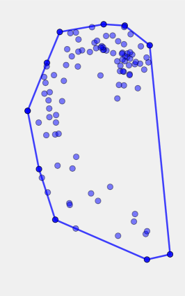
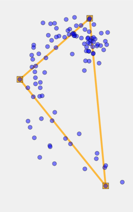
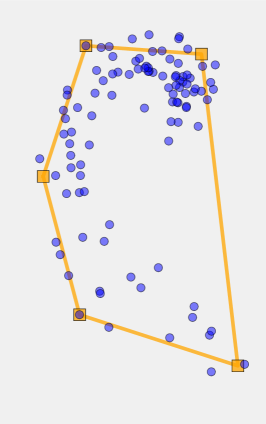
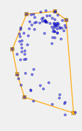
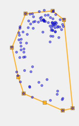
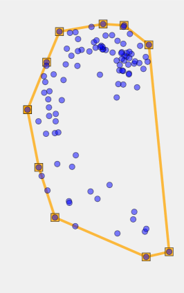
Cutler and Breiman [1] prove that, for , archetypes necessarily reside on the data convex hull. Moreover, if the hull has vertices and we choose , these vertices are the unique global minimizers of (4). Increasing the number of archetypes towards the number of vertices therefore improves the approximation of the convex hull (see Fig. 1).
These observations allow for a simplification of the problem in (4). Assume the vertices of the data convex hull were known and collected in . Archetypes could then be determined solely from matrix by solving the appropriately constrained problem
| (5) |
where is of size and of size . Once archetypes have been determined, coefficients for those data points not contained in can be computed in a second step. The appeal of this idea lies in the fact that typically so that solving (5) is less demanding than solving (4). Moreover, once is available, the problem in (4) needs only to be solved for matrix which requires less effort than estimating and simultaneously [2].
Alas, there is no free lunch! This approach requires to identify the vertices of the data convex hull which is expensive if the data are high dimensional [29]. Nevertheless, there are efficient heuristics for sampling the convex hull of a finite set of data [2, 6, 30, 31, 32, 33] and approximative archetypal analysis can indeed be computed for very large data matrices.
In this paper, we consider (5) as a vantage point for reasoning about the quality of archetypal analysis and related heuristics. Accordingly, we henceforth tacitly assume that the matrix containing the vertices of the data in was available. Moreover, to reduce clutter, we will drop the subscript of and and write both matrices as and , respectively.
IV Quality Estimates for AA
Looking at (5) we observe that the squared Frobenius norm may be rewritten as
| (6) |
where the identity matrix as well as the product matrix are both of size . However, while is of full rank , the rank of cannot exceed , because its columns are convex combinations of the columns of .
Hence, given (6) and assuming that , we can interpret archetypal analysis as the problem of finding a convexity constrained low-rank approximation of . In this section, we explore to what extent this insight allows bounding the quality of archetypal analysis and approximative heuristics. In particular, we note that
| (7) |
and ask how large or small can become for ?
IV-A Two general observations
To begin with, we show that a perfect low-rank approximation of is impossible. For the proof, we resort to geometric properties of the standard simplex to familiarize ourselves with arguments used later on.
Lemma 1.
Let be the identity matrix and and be two column stochastic matrices with . Then cannot be achieved.
Proof.
Note that the columns of lie the standard simplex whose vertices correspond to the columns of . In order for the difference of and to vanish, their corresponding columns must be equal
| (8) |
However, as a vertex of a convex set, is not a convex combination of other points in that set. Hence, in order for (8) to hold, every must be contained in the column set of . Yet, while there are columns in , there are only columns in . ∎
Having established that a perfect approximation of the unit matrix cannot be attained under the conditions studied here, we ask for the worst case. How bad can it possibly be?
Lemma 2.
Let , , and be given as above. The squared distance between and has an upper bound of
| (9) |
Proof.
The columns of and the columns of reside in the standard simplex which is a closed convex set. Any two vertices of are at a distance of and no two points in can be farther apart than two vertices. Therefore,
| (10) |
∎
This simple and straightforward result has consequences for archetypal analysis in general. Plugging it into (7) gives
| (11) |
and we realize that the number of vertices of the data convex hull may impact the quality of archetypal analysis. The more extremes there are, the higher the potential to err. However, the fewer extreme elements a data set contains, the better the chances of archetypal analysis to produce a good solution.
IV-B Two more specific observations
Curiously, the upper bound in (9) does not depend on the number of archetypes to be determined. Our next questions are therefore if it can be tightened and the parameter be incorporated.
First of all, we note that stochastic rank reduced approximations of the identity matrix can be understood geometrically. Recall that the columns of are convex combinations of the columns of which are -dimensional stochastic vectors that reside in . Approximating in terms of is therefore tantamount to placing vectors into such that its vertices can be approximated in terms of convex combinations over the .
Also, a good solution to (5) would mean so that . If one of the data vertices was reconstructed exactly, that is if , then therefore . However, is a vertex of and therefore not a convex combination of points in . Therefore one of the columns of must equal and the corresponding coefficient vector
In other words, selecting one of the of as an archetype is to place one of the of onto a vertex of .
Having established this, we can now analyze the SiVM heuristic for archetypal analysis. SiVM (simplex volume maximization) as introduced in [6] is a greedy search algorithm that determines data points in that are as far apart as possible and may therefore act as archetypes. In light of our discussion, this heuristic can thus be understood as implicitly placing the vectors onto of the vertices of the standard simplex .
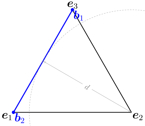
Say had been chosen this way. Then what is the minimal reconstruction error for any of the remaining vertices ? Again, we can argue geometrically. As the selected vertices form a subsimplex of , any remaining vertex would ideally be approximated by its closest point in . The distance between and corresponds to the height of the simplex formed by (see Fig. 2). Given the expression for the height of a standard simplex, we therefore have
| (12) |
This then establishes that, running SiVM for , we can achieve
| (13) |
In contrast to the quality estimate in (9), the one in (18) now depend on . It decreases for growing and, as expected, would drop to zero, if .
As a greedy selection mechanisms, SiVM is fast but suboptimal with respect to reconstruction accuracy. To see this, we next investigate what happens if the are not necessarily placed onto vertices of the standard simplex.

We begin by looking at the problem of computing a rank approximation of , that is, the problem of placing only a single vector into the standard simplex. Ideally, this vector would have a minimum distance to all the vertices and should therefore minimize
| (14) |
Deriving this objective function with respect to and equating the result to zero yields
| (15) |
Apparently, for , the optimal vector is (of course) the center point of . At the same time, the matrix of coefficients degenerates to a row vector which, as it must be stochastic, is the vector . We therefore have
| (16) |
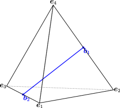
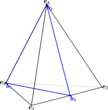
Next, we consider the problem of placing vectors into the standard simplex so as to approximate . Given our discussion so far, this problem can be approached in terms of subdividing the standard simplex into disjoint sub-simplices and placing one of the at the center of each of the resulting simplices. Put in simple terms, if we consider
| (17) |
such that and , the identity matrix can indeed be approximated with a reconstruction accuracy of
| (18) |
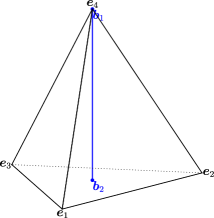
Interestingly, the quality estimate in (18) decreases linearly in . Again, and as expected, it will drop to zero, if . The examples in Fig. 3 show several configurations for which this reconstruction accuracy is achieved.
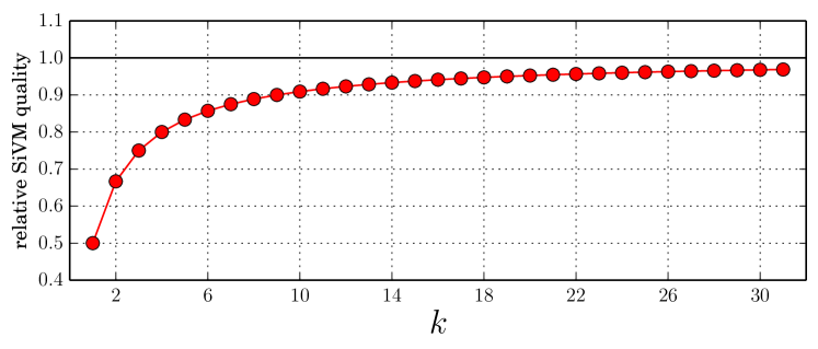
Finally, the results in (9) and (18) allow for estimating the relative reconstruction accuracy of the SiVM heuristic in comparison to conventional archetypal analysis. Figure 4 plots the ratio
| (19) |
as a function of . We observe that, for small choices of , the accuracy of SiVM quickly improves, exceeds for , and then slowly approaches the theoretically optimal performance of conventional AA if is increased further.
V Summary and Conclusion
In this note, we briefly reviewed the ideas behind archetypal analysis for data matrix factorization. We discussed geometric properties of solutions found by archetypal analysis and as to how far these allow for efficient heuristics for approximative AA. We then addressed the question of how to estimate the quality of AA algorithms. We showed that the problem of computing archetypal analysis can be reduced to the problem of computing a stochastic low rank approximation of the identity matrix. This point of view allowed us to characterize the optimal performance of SiVM heuristic as well as for conventional AA. Our results indicate that SiVM can provide robust solutions if a larger number of archetypes () are to be determined.
Glossary
Throughout this text, we are concerned with matrices and vectors over the field of real numbers .
Vectors are written as bold lower case letters () and their components in subscripted lower case italics (). is the vector of all zeros and is the vector of all ones.
Matrices are written using bold upper case letters () and doubly subscripted lower case italics () denote individual components. In order to express that a given matrix consists of column vectors, we also write where is the -th column of .
A vector is a stochastic vector, if for all and . For abbreviation, we write in order to indicate that is non-negative and use the inner product as a convenient shorthand for .
A matrix is column stochastic, if each of its column vectors is stochastic.
A set is called a convex set, if every point on the line segment between any two points in is also in , i.e. if
A vector is called a convex combination of vectors , if
Using matrix notation, we write where the matrix and the vector is a stochastic vector.
An extreme point of a convex set is any point that is not a convex combination of other points in . In other words, if is an extreme point and for and , then .
The convex hull of a set is the set of all possible convex combinations of points in , that is
A convex polytope is the convex hull of finitely many points, i.e. it is the set for . The extreme points of a polytope are called vertices. If is the set of all vertices of a polytope, then every point of the polytope can be expressed as a convex combination of the points in .
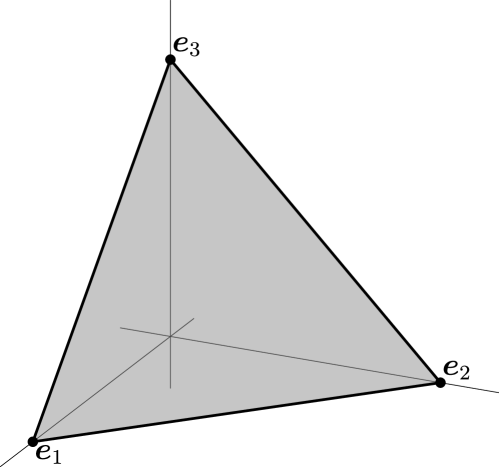
The standard simplex is the convex hull of the standard basis , that is
We note that the standard simplex is a polytope whose vertices correspond to the standard basis vectors (see Fig. 5) and that every stochastic vector resides within .
There are many useful results about the standard simplex . Among others, its side length is and its height is known to be
| (20) |
References
- [1] A. Cutler and L. Breiman, “Archetypal Analysis,” Technometrics, vol. 36, no. 4, pp. 338–347, 1994.
- [2] C. Bauckhage and C. Thurau, “Making Archetypal Analysis Practical,” in Pattern Recogntion, ser. LNCS, vol. 5748. Springer, 2009.
- [3] M. Eugster and F. Leisch, “Weighted and Robust Archetypal Analysis,” Computational Statistics & Data Analysis, vol. 55, no. 3, pp. 1215–1225, 2011.
- [4] M. Morup and L. Hansen, “Archetypal Analysis for Machine Learning and Data Mining,” Neurocomputing, vol. 80, pp. 54–63, 2012.
- [5] S. Seth and M. Eugster, “Probabilistic Archetypal Analysis,” arXiv:1312.7604v2 [stat.ML], 2014.
- [6] C. Thurau, K. Kersting, and C. Bauckhage, “Yes We Can – Simplex Volume Maximization for Descriptive Web-Scale Matrix Factorization,” in Proc. CIKM. ACM, 2010.
- [7] C. Thurau, K. Kersting, M. Wahabzada, and C. Bauckhage, “Convex Non-negative Matrix Factorization for Massive Datasets,” Knowledge and Information Systems, vol. 29, no. 2, pp. 457–478, 2011.
- [8] E. Stone and A. Cutler, “Archetypal Analysis of Spatio-temporal Dynamics,” Physica D, vol. 90, no. 3, pp. 209–224, 1996.
- [9] ——, “Exploring Archetypal Dynamics of Pattern Formation in Cellular Flames,” Physica D, vol. 161, no. 3–4, pp. 163–186, 2002.
- [10] B. Chan, D. Mitchell, and L. Cram, “Archetypal Analysis of Galaxy Spectra,” Monthly Notices of the Royal Astronomical Society, vol. 338, no. 3, pp. 790–795, 2003.
- [11] P. Huggins, L. Pachter, and B. Sturmfels, “Toward the Human Genotope,” Bulletin of Mathematical Biology, vol. 69, no. 8, pp. 2723–2735, 2007.
- [12] C. Römer, M. Wahabzada, A. Ballvora, F. Pinto, M. Rossini, C. Panigada, J. Behmann, J. Leon, C. Thurau, C. Bauckhage, K. Kersting, U. Rascher, and L. Plümer, “Early Drought Stress Detection in Cereals: Simplex Volume Maximization for Hyperspectral Image Analysis,” Functional Plant Biology, vol. 39, no. 11, pp. 878–890, 2012.
- [13] J. Thogersen, M. Morup, S. Damkiaer, S. Molin, and L. Jelsbak, “Archetypal Analysis of Diverse Pseudomonas Aeruginosa Transcriptomes Reveals Adaptation in Cystic Fibrosis Airways,” BMC Bioinformatics, vol. 14, no. 1, p. 279, 2013.
- [14] S. Li, P. Wang, and R. Carson, “Archetypal Analysis: A new Way to Segment Markets Based on Extreme Individuals,” in A Celebration of Ehrenberg and Bass: Marketing Knowledge, Discoveries and Contribution, R. Kennedy, Ed. ANZMAC, 2003, pp. 1674–1679.
- [15] C. Bauckhage and K. Manshaei, “Kernel Archetypal Analysis for Clustering Web Search Frequency Time Series,” in Proc. ICPR. IEEE, 2014.
- [16] R. Sifa, C. Bauckhage, and A. Drachen, “Archetypal Game Recommender Systems,” in Proc. KDML-LWA, 2014.
- [17] G. Porzio, G. Rafozini, and D. Vistocco, “Archetypal Analysis for Data Driven Benchmarking,” in Proc. Meeting of the Classification and Data Analysis Group (CLADAG) of the Italian Statistical Society, 2006.
- [18] M. Eugster, “Performance Profiles Based on Archetypal Athletes,” Int. J. of Performance Analysis in Sport, vol. 12, no. 1, pp. 166–187, 2012.
- [19] C. Seiler and K. Wohlrabe, “Archetypal Scientists,” J. of Infometrics, vol. 7, no. 2, pp. 345–356, 2013.
- [20] C. Thurau and A. Drachen, “Introducing Archetypal Analysis for Player Classification in Games,” in Proc. EPEX. ACM, 2001.
- [21] A. Drachen, R. Sifa, C. Bauckhage, and C. Thurau, “Guns, Swords, and Data: Clustering of Player Behavior in Computer Games in the Wild,” in Proc. CIG. IEEE, 2012.
- [22] R. Sifa and C. Bauckhage, “Archetypical Motion: Supervised Game Behavior Learning with Archetypal Analysis,” in Proc. CIG. IEEE, 2013.
- [23] S. Marinetti, L. Finesso, and E. Marsilio, “Matrix factorization methods: application to Thermal NDT/E,” in Proc. Int. Workshop Advances in Signal Processing for Non Destructive Evaluation of Materials, 2005.
- [24] C. Thurau and C. Bauckhage, “Archetypal Images in Large Photo Collections,” in Proc. ICSC. IEEE, 2009.
- [25] M. Cheema, A. Eweiwi, C. Thurau, and C. Bauckhage, “Action Recognition by Learning Discriminative Key Poses,” in Computer Vision Workshops (ICCV Workshops). IEEE, 2011.
- [26] S. Prabhakaran, S. Raman, J. Vogt, and V. Roth, “Automatic Model Selection in Archetype Analysis,” in Pattern Recognition, ser. LNCS, vol. 7476. Springer, 2012.
- [27] M. Asbach, D. Mauruschat, and B. Plinke, “Understanding Multi-spectral Images of Wood Particles with Matrix Factorization,” in Proc. Conf. on Optical Characterization of Materials, 2013.
- [28] Y. Xiong, W. Liu, D. Zhao, and X. Tang, “Face Recognition via Archetypal Hull Ranking,” in Proc. ICCV. IEEE, 2013.
- [29] M. de Berg, M. van Kreveld, M. Overmars, and O. Schwarzkopf, Computational Geometry. Springer, 2000.
- [30] K. Kersting, C. Bauckhage, C. Thurau, and M. Wahabzada, “Matrix Factorization as Search,” in Proc. ECML/PKDD, 2012.
- [31] M. Winter, “N-FINDR: An Algorithm for Fast and Autonomous Spectral Endmember Determination in Hyperspectral Data,” in Proc. Int. Conf. on Applied Geologic Remote Sensing, 1999.
- [32] C.-I. Chang, C.-C. Wu, W.-M. Liu, and Y.-C. Ouyang, “A New Growing Method for Simplex-Based Endmember Extraction Algorithm,” IEEE Trans. on Geoscience and Remote Sensing, vol. 44, no. 10, pp. 2804–2819, 2006.
- [33] L. Miao and H. Qi, “Endmember Extraction From Highly Mixed Data Using Minimum Volume Constrained Nonnegative Matrix Factorization,” IEEE Trans. on Geoscience and Remote Sensing, vol. 45, no. 3, pp. 765–777, 2007.