Cosmological perturbations in massive bigravity

Macarena Lagos    Pedro G. Ferreira
Abstract

We present a comprehensive analysis of classical scalar, vector and tensor cosmological perturbations in ghost-free massive bigravity. In particular, we find the full evolution equations and analytical solutions in a wide range of regimes. We show that there are viable cosmological backgrounds but, as has been found in the literature, these models generally have exponential instabilities in linear perturbation theory. However, it is possible to find stable scalar cosmological perturbations for a very particular choice of parameters. For this stable subclass of models we find that vector and tensor perturbations have growing solutions. We argue that special initial conditions are needed for tensor modes in order to have a viable model.

1 Introduction

Massive bigravity, as proposed by Hassan and Rosen in [1], is an alternative to general relativity, and an extension of the dRGT (de Rham, Gabadadze and Tolley) massive gravity [2]. One of the main attractions of this model is that it can predict viable cosmological homogeneous and isotropic solutions with late time self-acceleration without including a cosmological constant. Furthermore, if one assumes the presence of a large vacuum energy in this model, it has been argued that an appropriate value for the graviton’s mass may lead to screening of long wavelength modes, reconciling the value of the measured cosmological constant with quantum field theory [3]. As such, massive bigravity seems to be an appealing candidate for a theory of the universe.

Massive bigravity has five more degrees of freedom (dof) than general relativity (GR) – due to an extra massive graviton propagating – which could be a source of concern. Only recently has GR been shown to be well-behaved, i.e. that the initial value problem is sufficiently well posed that the theory can be considered classically predictive [4]. With an extra five degrees of freedom, it is conceivable that massive bigravity will not be as obliging. A possible hint of there being any problem would be the presence of classical instabilities and a natural first step would be to study linear cosmological perturbations. A first analysis of such perturbations has been undertaken in [5, 6, 7, 8], where unstable solutions on sub-horizon scales were found for some parameters of the theory in homogeneous and isotropic backgrounds111As of now, these type of backgrounds have been the only ones considered on cosmological studies of massive gravity.. A subsequent analysis in [9] identified a particular class of parameters that lead to stable solutions and, as such, might be used to construct a viable cosmology. In this paper, we undertake an independent analysis of the evolution and stability of linear cosmological perturbations using the gauge fixing method proposed in [10]. We confirm previous results for scalar perturbations but also analyse vector and tensor perturbations finding a number of interesting instabilities. Our results confirm the obvious: that it is a phenomenologically rich theory which needs to be studied in great detail if it is to be cosmologically considered on par with GR.

The outline of this paper is as follows. In section 2 we review the massive bigravity model. In section 3 we review the standard Friedmann-Robertson-Walker (FRW) cosmological background in the presence of a perfect fluid, and we find the equations of motion for first order cosmological perturbations. Here, we use the formalism developed in [10] to fix the gauge, simplify the problem, and to identify the physical degrees of freedom. In section 4, we study the evolution of the two physical scalar degrees of freedom, in section 5 we study vector perturbations, and in section 6 we study tensor perturbations. In section 7 we summarise our findings and discuss the prospects of massive bigravity as a viable theory of gravity and cosmology. Throughout this paper we will be using Planck units.

2 Bimetric Massive gravity

A linear theory of a massive spin-2 field in Minkowski space was proposed by Fierz and Pauli in 1939 [11]. It consists of a covariant quadratic action, known as the Fierz-Pauli action, describing a free massive spin-2 particle which propagates five degrees of freedom – namely, modes with helicity ±2plus-or-minus2\pm 2, ±1plus-or-minus1\pm 1 and 00. This action is the only possible instability-free quadratic action for a massive spin-2 particle [12]. In the presence of matter, the Fierz-Pauli action has the so-called van Dam, Veltman, Zakharov (vDVZ) discontinuity [13, 14], which arises when taking the massless limit; the helicity-0 mode couples to the trace of the stress-energy tensor, and therefore still propagates in the massless limit, where one would expect to only propagate the helicity ±2plus-or-minus2\pm 2 modes.

Non-linear massive gravitational theories (which reduce to the Fierz-Pauli action at the linear level) were studied extensively following the non-linear proposal by Vainshtein in 1972 [15]. It was then argued that non-linearities could cure the vDVZ discontinuity as these interactions would become comparable to the linear terms even for very weak fields, for small values of m𝑚m. Such non-linear interactions would give rise to a screening of the helicity-0 mode at observable scales, rendering the theory compatible with observational tests of gravity [15, 16]. Vainshtein’s model was flawed as it contained an instability, the so-called Boulware-Deser ghost [17], i.e. an extra scalar degree of freedom whose kinetic term had the wrong sign.

In 2010 major progress was made when a particular family of ghost-free interaction potentials was constructed by de Rham, Gabadadze and Tolley in [2] and confirmed to be ghost-free by Hassan and Rosen in [18] (see also [19]). dRGT massive gravity [20, 21, 22], as it is known, contains the space-time metric gμνsubscript𝑔𝜇𝜈g_{\mu\nu} as well as a fixed non-dynamical second metric fμνsubscript𝑓𝜇𝜈f_{\mu\nu}. A bimetric ghost-free extension of the dRGT massive gravity was proposed by Hassan and Rosen in [1] (see also [23]), where the new metric fμνsubscript𝑓𝜇𝜈f_{\mu\nu} is also dynamical. Concern on these types of theories may arise as for dRGT massive gravity some issues may been found (see [24, 25, 26, 27, 28, 29, 30] for related discussions). However, none of these problems have been seen in the bimetric model yet. For a more detailed review on massive gravity and its origins, see [3, 30].

In this paper, we will focus on the massive bigravity model proposed in [1]:

S=Mg22d4xgR(g)+Mf22d4xfR(f)m2Mg2d4xgn=04βnen(g1f)+Sm.𝑆superscriptsubscript𝑀𝑔22superscript𝑑4𝑥𝑔𝑅𝑔superscriptsubscript𝑀𝑓22superscript𝑑4𝑥𝑓𝑅𝑓superscript𝑚2superscriptsubscript𝑀𝑔2superscript𝑑4𝑥𝑔superscriptsubscript𝑛04subscript𝛽𝑛subscript𝑒𝑛superscript𝑔1𝑓subscript𝑆𝑚S=\;\frac{M_{g}^{2}}{2}\int d^{4}x\sqrt{-g}R(g)+\frac{M_{f}^{2}}{2}\int d^{4}x\sqrt{-f}R(f)-m^{2}M_{g}^{2}\int d^{4}x\sqrt{-g}\sum_{n=0}^{4}\beta_{n}e_{n}\left(\sqrt{g^{-1}f}\right)+S_{m}. (2.1)

In this action there are two dynamical metric fields gμνsubscript𝑔𝜇𝜈g_{\mu\nu} and fμνsubscript𝑓𝜇𝜈f_{\mu\nu}, with their associated Ricci scalars R(g)𝑅𝑔R(g) and R(f)𝑅𝑓R(f), respectively, along with a coupling to matter, Smsubscript𝑆𝑚S_{m}. In addition, this action contains interactions between both metrics that preserve general covariance, and are expressed in terms of the functions en(g1f)subscript𝑒𝑛superscript𝑔1𝑓e_{n}\left(\sqrt{g^{-1}f}\right), which correspond to the elementary symmetric polynomials of the eigenvalues λnsubscript𝜆𝑛\lambda_{n} of the matrix g1fsuperscript𝑔1𝑓\sqrt{g^{-1}f}, which satisfies g1fg1f=gμλfλνsuperscript𝑔1𝑓superscript𝑔1𝑓superscript𝑔𝜇𝜆subscript𝑓𝜆𝜈\sqrt{g^{-1}f}\sqrt{g^{-1}f}=g^{\mu\lambda}f_{\lambda\nu}. Note that there is an ambiguity in g1fsuperscript𝑔1𝑓\sqrt{g^{-1}f}, as different matrices may result in gμλfλνsuperscript𝑔𝜇𝜆subscript𝑓𝜆𝜈g^{\mu\lambda}f_{\lambda\nu} when squared. Finally, βnsubscript𝛽𝑛\beta_{n} are free dimensionless coefficients while Mgsubscript𝑀𝑔M_{g}, Mfsubscript𝑀𝑓M_{f}, and m𝑚m are mass scales. For simplicity, we will be considering the case where matter is minimally coupled to gμνsubscript𝑔𝜇𝜈g_{\mu\nu} only, and therefore gμνsubscript𝑔𝜇𝜈g_{\mu\nu} will be describing the space-time evolution.

As shown in [22], the equations of motion for gμνsubscript𝑔𝜇𝜈g_{\mu\nu} and fμνsubscript𝑓𝜇𝜈f_{\mu\nu} are:

R(g)μν12gμνR(g)+m22n=03(1)nβn[gμλY(n)νλ(g1f)+gνλY(n)μλ(g1f)]=TμνMg2,𝑅subscript𝑔𝜇𝜈12subscript𝑔𝜇𝜈𝑅𝑔superscript𝑚22superscriptsubscript𝑛03superscript1𝑛subscript𝛽𝑛delimited-[]subscript𝑔𝜇𝜆subscriptsuperscript𝑌𝜆𝑛𝜈superscript𝑔1𝑓subscript𝑔𝜈𝜆subscriptsuperscript𝑌𝜆𝑛𝜇superscript𝑔1𝑓subscript𝑇𝜇𝜈superscriptsubscript𝑀𝑔2\displaystyle\;R(g)_{\mu\nu}-\frac{1}{2}g_{\mu\nu}R(g)+\frac{m^{2}}{2}\sum_{n=0}^{3}(-1)^{n}\beta_{n}\left[g_{\mu\lambda}Y^{\lambda}_{(n)\nu}\left(\sqrt{g^{-1}f}\right)+g_{\nu\lambda}Y^{\lambda}_{(n)\mu}\left(\sqrt{g^{-1}f}\right)\right]=\frac{T_{\mu\nu}}{M_{g}^{2}}, (2.2)
R(f)μν12fμνR(f)+m22M2n=03(1)nβ4n[fμλY(n)νλ(f1g)+fνλY(n)μλ(f1g)]=0,𝑅subscript𝑓𝜇𝜈12subscript𝑓𝜇𝜈𝑅𝑓superscript𝑚22superscriptsubscript𝑀2superscriptsubscript𝑛03superscript1𝑛subscript𝛽4𝑛delimited-[]subscript𝑓𝜇𝜆subscriptsuperscript𝑌𝜆𝑛𝜈superscript𝑓1𝑔subscript𝑓𝜈𝜆subscriptsuperscript𝑌𝜆𝑛𝜇superscript𝑓1𝑔0\displaystyle\;R(f)_{\mu\nu}-\frac{1}{2}f_{\mu\nu}R(f)+\frac{m^{2}}{2M_{*}^{2}}\sum_{n=0}^{3}(-1)^{n}\beta_{4-n}\left[f_{\mu\lambda}Y^{\lambda}_{(n)\nu}\left(\sqrt{f^{-1}g}\right)+f_{\nu\lambda}Y^{\lambda}_{(n)\mu}\left(\sqrt{f^{-1}g}\right)\right]=0, (2.3)

where M2Mf2/Mg2superscriptsubscript𝑀2superscriptsubscript𝑀𝑓2superscriptsubscript𝑀𝑔2M_{*}^{2}\equiv M_{f}^{2}/M_{g}^{2}, and Tμνsuperscript𝑇𝜇𝜈T^{\mu\nu} is the matter stress-energy tensor, and where we have used the following relation for the interaction terms:

gn=04βnen(g1f)=gn=04βne4n(f1g)det(g1f)=fn=04β4nen(f1g),𝑔superscriptsubscript𝑛04subscript𝛽𝑛subscript𝑒𝑛superscript𝑔1𝑓𝑔superscriptsubscript𝑛04subscript𝛽𝑛subscript𝑒4𝑛superscript𝑓1𝑔superscript𝑔1𝑓𝑓superscriptsubscript𝑛04subscript𝛽4𝑛subscript𝑒𝑛superscript𝑓1𝑔\sqrt{-g}\sum_{n=0}^{4}\beta_{n}e_{n}\left(\sqrt{g^{-1}f}\right)=\sqrt{-g}\sum_{n=0}^{4}\beta_{n}\frac{e_{4-n}\left(\sqrt{f^{-1}g}\right)}{\det\left(\sqrt{g^{-1}f}\right)}=\sqrt{-f}\sum_{n=0}^{4}\beta_{4-n}e_{n}\left(\sqrt{f^{-1}g}\right), (2.4)

where the matrix f1gsuperscript𝑓1𝑔\sqrt{f^{-1}g} is the inverse of g1fsuperscript𝑔1𝑓\sqrt{g^{-1}f}. Note that to satisfy this relation we need to have gdet(g1f)=f𝑔superscript𝑔1𝑓𝑓\sqrt{-g}\det(\sqrt{g^{-1}f})=\sqrt{-f}. Otherwise, we would have a minus sign in the RHS of eq. (2.4), and therefore a minus sign in the interaction terms of eq. (2.3). In addition, matrices Y(n)μλ(𝕏)subscriptsuperscript𝑌𝜆𝑛𝜇𝕏Y^{\lambda}_{(n)\mu}(\mathbb{X}) are defined as:

Y(0)=subscript𝑌0absent\displaystyle Y_{(0)}= 𝕀,𝕀\displaystyle\mathbb{I},
Y(1)=subscript𝑌1absent\displaystyle Y_{(1)}= 𝕏𝕀[𝕏],𝕏𝕀delimited-[]𝕏\displaystyle\mathbb{X}-\mathbb{I}[\mathbb{X}],
Y(2)=subscript𝑌2absent\displaystyle Y_{(2)}= 𝕏2𝕏[𝕏]+12𝕀([𝕏]2[𝕏2]),superscript𝕏2𝕏delimited-[]𝕏12𝕀superscriptdelimited-[]𝕏2delimited-[]superscript𝕏2\displaystyle\mathbb{X}^{2}-\mathbb{X}[\mathbb{X}]+\frac{1}{2}\mathbb{I}\left([\mathbb{X}]^{2}-[\mathbb{X}^{2}]\right),
Y(3)=subscript𝑌3absent\displaystyle Y_{(3)}= 𝕏3𝕏2[𝕏]+12𝕏([𝕏]2[𝕏2])16𝕀([𝕏]33[𝕏][𝕏2]+2[𝕏3]),superscript𝕏3superscript𝕏2delimited-[]𝕏12𝕏superscriptdelimited-[]𝕏2delimited-[]superscript𝕏216𝕀superscriptdelimited-[]𝕏33delimited-[]𝕏delimited-[]superscript𝕏22delimited-[]superscript𝕏3\displaystyle\mathbb{X}^{3}-\mathbb{X}^{2}[\mathbb{X}]+\frac{1}{2}\mathbb{X}\left([\mathbb{X}]^{2}-[\mathbb{X}^{2}]\right)-\frac{1}{6}\mathbb{I}\left([\mathbb{X}]^{3}-3[\mathbb{X}][\mathbb{X}^{2}]+2[\mathbb{X}^{3}]\right), (2.5)

where 𝕀𝕀\mathbb{I} is the identity matrix and [𝕏]delimited-[]𝕏[\mathbb{X}] stands for the trace of the matrix 𝕏𝕏\mathbb{X}. We must also add a matter equation which, in this case, will correspond to the local conservation of energy-momentum:

gμTμν=0,subscriptsuperscript𝜇𝑔subscript𝑇𝜇𝜈0\nabla^{\mu}_{g}T_{\mu\nu}=0, (2.6)

where gμsubscriptsuperscript𝜇𝑔\nabla^{\mu}_{g} is the covariant derivative with respect to the metric gμνsubscript𝑔𝜇𝜈g_{\mu\nu}.

3 Cosmological perturbations

In this section we first review previous results on solutions for homogeneous and isotropic universes in massive bigravity. We then consider general linear cosmological perturbations using the standard classification of scalar, vector and tensor [31].

3.1 Background

For simplicity we will assume that both metrics share the same characteristics: homogeneous, isotropic and flat:

dsf2𝑑superscriptsubscript𝑠𝑓2\displaystyle ds_{f}^{2} =Y(τ)2[X(τ)2dτ2+δijdxidxj],absent𝑌superscript𝜏2delimited-[]𝑋superscript𝜏2𝑑superscript𝜏2subscript𝛿𝑖𝑗𝑑superscript𝑥𝑖𝑑superscript𝑥𝑗\displaystyle=Y(\tau)^{2}[-X(\tau)^{2}d\tau^{2}+\delta_{ij}dx^{i}dx^{j}], (3.1)
dsg2𝑑superscriptsubscript𝑠𝑔2\displaystyle ds_{g}^{2} =a(τ)2[dτ2+δijdxidxj],absent𝑎superscript𝜏2delimited-[]𝑑superscript𝜏2subscript𝛿𝑖𝑗𝑑superscript𝑥𝑖𝑑superscript𝑥𝑗\displaystyle=a(\tau)^{2}[-d\tau^{2}+\delta_{ij}dx^{i}dx^{j}], (3.2)

where τ𝜏\tau is the conformal time, a(τ)𝑎𝜏a(\tau) is the scale factor of the space-time metric, and X(τ)𝑋𝜏X(\tau) with Y(τ)𝑌𝜏Y(\tau) describe the evolution of the metric fμνsubscript𝑓𝜇𝜈f_{\mu\nu}.

In addition, we will assume the type of matter coupled to gravity to be a perfect fluid:

Tμ=ν(p0+ρ0)u0μu0ν+p0δμ,νT^{\mu}{}_{\nu}=(p_{0}+\rho_{0})u^{\mu}_{0}u_{0\nu}+p_{0}\delta^{\mu}{}_{\nu}, (3.3)

where p0=p0(τ)subscript𝑝0subscript𝑝0𝜏p_{0}=p_{0}(\tau) is the pressure of the fluid, ρ0=ρ0(τ)subscript𝜌0subscript𝜌0𝜏\rho_{0}=\rho_{0}(\tau) its rest energy density and u0μ=(1/a,0,0,0)subscriptsuperscript𝑢𝜇01𝑎000u^{\mu}_{0}=(1/a,0,0,0) its isotropic 4-velocity.

If we replace eq. (3.1)-(3.3) into eq. (2.2)-(2.3), we find the following equations of motion:

2superscript2\displaystyle\mathcal{H}^{2} =a23[ρ0Mg2+m2(β0+3β1N+3β2N2+β3N3)],absentsuperscript𝑎23delimited-[]subscript𝜌0superscriptsubscript𝑀𝑔2superscript𝑚2subscript𝛽03subscript𝛽1𝑁3subscript𝛽2superscript𝑁2subscript𝛽3superscript𝑁3\displaystyle=\frac{a^{2}}{3}\left[\frac{\rho_{0}}{M_{g}^{2}}+m^{2}\left(\beta_{0}+3\beta_{1}N+3\beta_{2}N^{2}+\beta_{3}N^{3}\right)\right], (3.4)
superscript\displaystyle\mathcal{H}^{\prime} =a22[p0Mg22a2+m2(β0+β1N[2+X]+β2N2[1+2X]+β3N3X)],absentsuperscript𝑎22delimited-[]subscript𝑝0superscriptsubscript𝑀𝑔2superscript2superscript𝑎2superscript𝑚2subscript𝛽0subscript𝛽1𝑁delimited-[]2𝑋subscript𝛽2superscript𝑁2delimited-[]12𝑋subscript𝛽3superscript𝑁3𝑋\displaystyle=\frac{a^{2}}{2}\left[-\frac{p_{0}}{M_{g}^{2}}-\frac{\mathcal{H}^{2}}{a^{2}}+m^{2}\left(\beta_{0}+\beta_{1}N\left[2+X\right]+\beta_{2}N^{2}\left[1+2X\right]+\beta_{3}N^{3}X\right)\right], (3.5)
h2superscript2\displaystyle h^{2} =a23(X2N)ν2(β1+3β2N+3β3N2+β4N3),absentsuperscript𝑎23superscript𝑋2𝑁superscript𝜈2subscript𝛽13subscript𝛽2𝑁3subscript𝛽3superscript𝑁2subscript𝛽4superscript𝑁3\displaystyle=\frac{a^{2}}{3}\left(\frac{X^{2}}{N}\right)\nu^{2}\left(\beta_{1}+3\beta_{2}N+3\beta_{3}N^{2}+\beta_{4}N^{3}\right), (3.6)
hsuperscript\displaystyle h^{\prime} =a22[2a2hxhh2a2+(XN)ν2(β1+β2N[2+X]+β3N2[1+2X]+β4N3X)]absentsuperscript𝑎22delimited-[]2superscript𝑎2subscript𝑥superscript2superscript𝑎2𝑋𝑁superscript𝜈2subscript𝛽1subscript𝛽2𝑁delimited-[]2𝑋subscript𝛽3superscript𝑁2delimited-[]12𝑋subscript𝛽4superscript𝑁3𝑋\displaystyle=\frac{a^{2}}{2}\left[\frac{2}{a^{2}}h_{x}h-\frac{h^{2}}{a^{2}}+\left(\frac{X}{N}\right)\nu^{2}\left(\beta_{1}+\beta_{2}N[2+X]+\beta_{3}N^{2}[1+2X]+\beta_{4}N^{3}X\right)\right] (3.7)

where it is implicit that all variables depend only on τ𝜏\tau, all primes represent conformal time derivatives, and we have defined =a/asuperscript𝑎𝑎\mathcal{H}=a^{\prime}/a, h=Y/Ysuperscript𝑌𝑌h=Y^{\prime}/Y, hx=X/Xsubscript𝑥superscript𝑋𝑋h_{x}=X^{\prime}/X, ν=m/M𝜈𝑚subscript𝑀\nu=m/M_{*}, and N=Y/a𝑁𝑌𝑎N=Y/a. Note that the parameter Msubscript𝑀M_{*} is redundant, as we can rescale the metric fμνsubscript𝑓𝜇𝜈f_{\mu\nu} to make Msubscript𝑀M_{*} take any value we want and redefine β𝛽\betas such that the action remains invariant. For simplicity, from now on we will use M=1subscript𝑀1M_{*}=1.

It is important to note that in order to obtain the previous equations, we had to make a choice for the matrix g1fsuperscript𝑔1𝑓\sqrt{g^{-1}f}. For simplicity, we have chosen the diagonal form: g1f=diag(NX,N,N,N)superscript𝑔1𝑓diag𝑁𝑋𝑁𝑁𝑁\sqrt{g^{-1}f}=\mbox{diag}\left(NX,N,N,N\right). As we will explain later, some solutions allow X𝑋X to change sign, and therefore this matrix can change sign at some point. Then, in order to satisfy gdet(g1f)=f𝑔superscript𝑔1𝑓𝑓\sqrt{-g}\det(\sqrt{g^{-1}f})=\sqrt{-f}, and therefore eq. (2.4), we need to make the unconventional (multivalued) choice of g𝑔\sqrt{-g} and f𝑓\sqrt{-f} without absolute values, allowing them to change signs. As explained in [32, 33] if g1fsuperscript𝑔1𝑓\sqrt{g^{-1}f} can change sign we can find continuous solutions through singularities in fμνsubscript𝑓𝜇𝜈f_{\mu\nu}.

We also have the matter equation of motion:

ρ0=3(ρ0+p0),superscriptsubscript𝜌03subscript𝜌0subscript𝑝0\rho_{0}^{\prime}=-3\mathcal{H}(\rho_{0}+p_{0}), (3.8)

which has the standard form, as matter has been minimally coupled to the metric gμνsubscript𝑔𝜇𝜈g_{\mu\nu}. In addition, we have Bianchi constraints for both metrics, resulting from the Bianchi identities and the local conservation of the matter stress-energy tensor. However, due to the diffeomorphism invariance, they are both equivalent, so we have only one relevant Bianchi constraint, given in this case by:

(Xh)(β1+2β2N+β3N2)=0.𝑋subscript𝛽12subscript𝛽2𝑁subscript𝛽3superscript𝑁20\left(X\mathcal{H}-h\right)\left(\beta_{1}+2\beta_{2}N+\beta_{3}N^{2}\right)=0. (3.9)

We can easily identify two cases for the solutions:

(β1+2β2N+β3N2)=0subscript𝛽12subscript𝛽2𝑁subscript𝛽3superscript𝑁20\left(\beta_{1}+2\beta_{2}N+\beta_{3}N^{2}\right)=0:

This case leads to a constant N=N¯𝑁¯𝑁N=\bar{N}, such that

β1+2β2N¯+β3N¯2=0.subscript𝛽12subscript𝛽2¯𝑁subscript𝛽3superscript¯𝑁20\beta_{1}+2\beta_{2}\bar{N}+\beta_{3}\bar{N}^{2}=0. (3.10)

As a consequence, =h\mathcal{H}=h and the Friedmann equation becomes:

2=a23[ρ0Mg2+Λ];Λ=m2(β0+3β1N¯+3β2N¯2+β3N¯3),formulae-sequencesuperscript2superscript𝑎23delimited-[]subscript𝜌0superscriptsubscript𝑀𝑔2ΛΛsuperscript𝑚2subscript𝛽03subscript𝛽1¯𝑁3subscript𝛽2superscript¯𝑁2subscript𝛽3superscript¯𝑁3\mathcal{H}^{2}=\frac{a^{2}}{3}\left[\frac{\rho_{0}}{M_{g}^{2}}+\Lambda\right];\;\Lambda=m^{2}\left(\beta_{0}+3\beta_{1}\bar{N}+3\beta_{2}\bar{N}^{2}+\beta_{3}\bar{N}^{3}\right), (3.11)

which corresponds to general relativity with a cosmological constant. This case is not particularly interesting at the background level as it does not bring new features. Furthermore, as pointed out in [34], when studying first order perturbations, the interaction terms between gμνsubscript𝑔𝜇𝜈g_{\mu\nu} and fμνsubscript𝑓𝜇𝜈f_{\mu\nu} vanish when imposing the constraint (3.10), and the model results in just two copies of general relativity.

(Xh)=0𝑋0\left(X\mathcal{H}-h\right)=0:

This constraint can be replaced into eq. (3.6), and then compared to eq. (3.4), to find the following consistency equation:

ρ~ρm2=β1N+3β2β0+3N(β3β1)+N2(β43β2)N3β3;ρ=ρ0/Mg2,formulae-sequence~𝜌subscript𝜌superscript𝑚2subscript𝛽1𝑁3subscript𝛽2subscript𝛽03𝑁subscript𝛽3subscript𝛽1superscript𝑁2subscript𝛽43subscript𝛽2superscript𝑁3subscript𝛽3subscript𝜌subscript𝜌0superscriptsubscript𝑀𝑔2\tilde{\rho}\equiv\frac{\rho_{*}}{m^{2}}=\frac{\beta_{1}}{N}+3\beta_{2}-\beta_{0}+3N(\beta_{3}-\beta_{1})+N^{2}(\beta_{4}-3\beta_{2})-N^{3}\beta_{3};\quad\rho_{*}=\rho_{0}/M_{g}^{2}, (3.12)

which relates N𝑁N and the density ρ0subscript𝜌0\rho_{0}.

For a standard equation of state p0=wρ0subscript𝑝0𝑤subscript𝜌0p_{0}=w\rho_{0} (with w𝑤w constant), according to eq. (3.12), at late times (ρ~1much-less-than~𝜌1\tilde{\rho}\ll 1), N𝑁N will approach a constant value, and both metrics enter an accelerated de-Sitter phase. However, at early times (ρ~1much-greater-than~𝜌1\tilde{\rho}\gg 1), two types of behaviours can be identified: one where N1much-less-than𝑁1N\ll 1 (and β10subscript𝛽10\beta_{1}\not=0) and another where N1much-greater-than𝑁1N\gg 1. The branch characterised by N1much-less-than𝑁1N\ll 1 at early times will be called expanding branch, as in this case both metrics expand in time. While the branch characterised by N1much-greater-than𝑁1N\gg 1 will be called bouncing branch, as in this case gμνsubscript𝑔𝜇𝜈g_{\mu\nu} expands but fμνsubscript𝑓𝜇𝜈f_{\mu\nu} bounces.

The expanding branch is usually identified as the physical one as, in this case, the contribution of the graviton mass to the Friedmann equation will always be small (for appropriate choices of parameters), as expected. However, in the bouncing branch, the contribution of the graviton mass may be comparable to the matter energy density ρ0subscript𝜌0\rho_{0} at early times. Furthermore, in the bouncing branch, if w>0𝑤0w>0 at early times, then X<0𝑋0X<0 at early times, and tend to X=1𝑋1X=1 at late times. This means that X𝑋X crosses a zero point, where f00=0subscript𝑓000f_{00}=0, and therefore fμν1subscriptsuperscript𝑓1𝜇𝜈f^{-1}_{\mu\nu} diverges. At this point also det(g1f)=0superscript𝑔1𝑓0\det(\sqrt{g^{-1}f})=0. As explained in [32, 33], this divergence stays hidden from the matter sector as gμνsubscript𝑔𝜇𝜈g_{\mu\nu} does not experience any divergence, and the corresponding vielbein fields are continuous through this point. We confirm this at the level of the background, where no divergence is present in the set of equations of motion eq. (3.4)-(3.7), nor in their solutions222One might worry about eq. (3.7), as the first term in the RHS contains hxsubscript𝑥h_{x}, which diverges when X=0𝑋0X=0. However, the full relevant quantity in that equation is hxhsubscript𝑥h_{x}h, which is finite. This can be seen from eq. (3.6), where we observe that hXproportional-to𝑋h\propto X, cancelling the X𝑋X in the denominator of hxsubscript𝑥h_{x} and rendering the relevant term finite.. In addition, in the next sections we find non-divergent solutions for linear perturbations through this point. Therefore, our results suggest that this divergence might have a mathematical origin instead of a physical one333The Ricci scalar associated to the metric fμνsubscript𝑓𝜇𝜈f_{\mu\nu} diverges, while the one for gμνsubscript𝑔𝜇𝜈g_{\mu\nu} does not. Given that the latter one represents the space-time metric, it will determine the relevant physical properties of space-time. Furthermore, the Ricci scalar of fμνsubscript𝑓𝜇𝜈f_{\mu\nu} will always appear multiplied by the determinant of fμνsubscript𝑓𝜇𝜈f_{\mu\nu}, rendering it finite.. Then, even though solutions in the bouncing branch are exotic, they will be analysed in this paper at the level of perturbations. However, it is clear to us that further research is needed to understand completely the nature of this branch.

Throughout this paper we will focus on the second branch of solutions satisfying X=h𝑋X\mathcal{H}=h, as this one brings relevant modifications to general relativity. Background solutions and viable cosmologies in this branch have been studied in detail in [35, 36, 37, 38, 39, 34]. Given these results, the next logical step is the study of cosmological perturbations in this background. We will use the standard tensor-vector-scalar decomposition, and find the relevant equations of motion for these three types of perturbations.

3.2 Scalar perturbations

Let us consider linear scalar perturbations [9, 5, 6, 7, 8]. We use the following Ansatz for the perturbed metrics:

dsf2𝑑superscriptsubscript𝑠𝑓2\displaystyle ds_{f}^{2} =Y2[X2(1+2ϕ1)dτ2+2B1,iXdxidτ+[(12ψ1)δij+2E1,ij]dxidxj],absentsuperscript𝑌2delimited-[]superscript𝑋212subscriptitalic-ϕ1𝑑superscript𝜏22subscript𝐵1𝑖𝑋𝑑superscript𝑥𝑖𝑑𝜏delimited-[]12subscript𝜓1subscript𝛿𝑖𝑗2subscript𝐸1𝑖𝑗𝑑superscript𝑥𝑖𝑑superscript𝑥𝑗\displaystyle=Y^{2}[-X^{2}(1+2\phi_{1})d\tau^{2}+2B_{1,i}Xdx^{i}d\tau+[(1-2\psi_{1})\delta_{ij}+2E_{1,ij}]dx^{i}dx^{j}], (3.13)
dsg2𝑑superscriptsubscript𝑠𝑔2\displaystyle ds_{g}^{2} =a2[(1+2ϕ2)dτ2+2B2,idxidτ+[(12ψ2)δij+2E2,ij]dxidxj],absentsuperscript𝑎2delimited-[]12subscriptitalic-ϕ2𝑑superscript𝜏22subscript𝐵2𝑖𝑑superscript𝑥𝑖𝑑𝜏delimited-[]12subscript𝜓2subscript𝛿𝑖𝑗2subscript𝐸2𝑖𝑗𝑑superscript𝑥𝑖𝑑superscript𝑥𝑗\displaystyle=a^{2}[-(1+2\phi_{2})d\tau^{2}+2B_{2,i}dx^{i}d\tau+[(1-2\psi_{2})\delta_{ij}+2E_{2,ij}]dx^{i}dx^{j}], (3.14)

where dsf2𝑑superscriptsubscript𝑠𝑓2ds_{f}^{2} and dsg2𝑑superscriptsubscript𝑠𝑔2ds_{g}^{2} are the line elements for the metrics fμνsubscript𝑓𝜇𝜈f_{\mu\nu} and gμνsubscript𝑔𝜇𝜈g_{\mu\nu} respectively. We read from here that we have four scalar perturbation fields for each metric: ϕ1subscriptitalic-ϕ1\phi_{1}, B1subscript𝐵1B_{1}, E1subscript𝐸1E_{1}, ψ1subscript𝜓1\psi_{1} for fμνsubscript𝑓𝜇𝜈f_{\mu\nu} and ϕ2subscriptitalic-ϕ2\phi_{2}, B2subscript𝐵2B_{2}, E2subscript𝐸2E_{2}, ψ2subscript𝜓2\psi_{2} for gμνsubscript𝑔𝜇𝜈g_{\mu\nu}.

For matter, we have a perfect fluid with an equation of state p=wρ𝑝𝑤𝜌p=w\rho, and therefore the perturbed stress-energy tensor coupled to these scalar perturbations can be written as:

δT0=0\displaystyle\delta T^{0}{}_{0}= (ρ0+p0)(3ψ2E2,iiχ,ii),\displaystyle-(\rho_{0}+p_{0})(3\psi_{2}-E_{2,ii}-\chi_{,ii}),
δTi=0\displaystyle\delta T^{i}{}_{0}= (ρ0+p0)χ,i,\displaystyle-(\rho_{0}+p_{0})\chi^{\prime}_{,i},
δT0=i\displaystyle\delta T^{0}{}_{i}= (ρ0+p0)(B2,i+χ,i),\displaystyle(\rho_{0}+p_{0})(B_{2,i}+\chi^{\prime}_{,i}),
δTi=j\displaystyle\delta T^{i}{}_{j}= w(ρ0+p0)(3ψ2E2,llχ,ll)δi.j\displaystyle w(\rho_{0}+p_{0})(3\psi_{2}-E_{2,ll}-\chi_{,ll})\delta^{i}{}_{j}. (3.15)

Note that we describe matter perturbations with only one scalar field χ𝜒\chi, in a non-conventional but useful way proposed in [31]. Consequently, we have nine scalar fields describing first order perturbations in this theory. As we will see later, from these nine fields there will be only two propagating physical degrees of freedom: one coming from matter perturbations and another one from the helicity-0 mode of the massive graviton. All the other seven scalar fields are simply auxiliary fields, i.e. they appear without time derivatives and therefore they are not physical dynamical fields. This unconventional description for perfect fluid perturbations is useful in order to apply the tools developed in [10] to eliminate ambiguities related to the gauge-symmetry present in the theory.

The action given in eq. (2.1) is invariant under diffeomorphisms, and the nine perturbation scalar fields in the model transform under this symmetry as:

ϕ~2=ϕ2ξ0ξ0,ψ~2=ψ2+ξ0,B~2=B2+ξ0ξ,formulae-sequencesubscript~italic-ϕ2subscriptitalic-ϕ2superscript𝜉0superscript𝜉superscript0formulae-sequencesubscript~𝜓2subscript𝜓2superscript𝜉0subscript~𝐵2subscript𝐵2superscript𝜉0superscript𝜉\displaystyle\tilde{\phi}_{2}=\phi_{2}-\mathcal{H}\xi^{0}-\xi^{0^{\prime}},\;\tilde{\psi}_{2}=\psi_{2}+\mathcal{H}\xi^{0},\;\tilde{B}_{2}=B_{2}+\xi^{0}-\xi^{\prime},
E~2=E2ξ,ϕ~1=ϕ1[h+hx]ξ0ξ0,formulae-sequencesubscript~𝐸2subscript𝐸2𝜉subscript~italic-ϕ1subscriptitalic-ϕ1delimited-[]subscript𝑥superscript𝜉0superscript𝜉superscript0\displaystyle\tilde{E}_{2}=E_{2}-\xi,\;\tilde{\phi}_{1}=\phi_{1}-\left[h+h_{x}\right]\xi^{0}-\xi^{0^{\prime}},
ψ~1=ψ1+hξ0,B~1=B1ξX+ξ0X,E~1=E1ξ,formulae-sequencesubscript~𝜓1subscript𝜓1superscript𝜉0formulae-sequencesubscript~𝐵1subscript𝐵1superscript𝜉𝑋superscript𝜉0𝑋subscript~𝐸1subscript𝐸1𝜉\displaystyle\tilde{\psi}_{1}=\psi_{1}+h\xi^{0},\;\tilde{B}_{1}=B_{1}-\frac{\xi^{\prime}}{X}+\xi^{0}X,\;\tilde{E}_{1}=E_{1}-\xi,
χ~=χ+ξ,~𝜒𝜒𝜉\displaystyle\tilde{\chi}=\chi+\xi, (3.16)

where ξ𝜉\xi and ξ0superscript𝜉0\xi^{0} are the two scalar gauge parameters. As these fields are gauge-dependent, anything you calculate from them will depend on your gauge-choice. This ambiguity is usually eliminated by defining a new set of independent gauge-invariant scalar fields. In this paper we will approach this problem by fixing the gauge in a convenient way, as in [10]. First, we look at the Noether identities associated to the gauge symmetry:

ϕ1ϕ1[h+hx]+ψ1h+B1X+ϕ2+(ψ2ϕ2)+B2=0,superscriptsubscriptsubscriptitalic-ϕ1subscriptsubscriptitalic-ϕ1delimited-[]subscript𝑥subscriptsubscript𝜓1subscriptsubscript𝐵1𝑋superscriptsubscriptsubscriptitalic-ϕ2subscriptsubscript𝜓2subscriptsubscriptitalic-ϕ2subscriptsubscript𝐵20\displaystyle\mathcal{E}_{\phi_{1}}^{\prime}-\mathcal{E}_{\phi_{1}}\left[h+h_{x}\right]+\mathcal{E}_{\psi_{1}}h+\mathcal{E}_{B_{1}}X+\mathcal{E}_{\phi_{2}}^{\prime}+\left(\mathcal{E}_{\psi_{2}}-\mathcal{E}_{\phi_{2}}\right)\mathcal{H}+\mathcal{E}_{B_{2}}=0,
ξE1+(B1X)E2+B2=0,subscript𝜉subscriptsubscript𝐸1superscriptsubscriptsubscript𝐵1𝑋subscriptsubscript𝐸2superscriptsubscriptsubscript𝐵20\displaystyle\mathcal{E}_{\xi}-\mathcal{E}_{E_{1}}+\left(\frac{\mathcal{E}_{B_{1}}}{X}\right)^{\prime}-\mathcal{E}_{E_{2}}+\mathcal{E}_{B_{2}}^{\prime}=0, (3.17)

where we have denoted xsubscript𝑥\mathcal{E}_{x} as the equation of motion for the field x𝑥x. From here we can recognise those fields with redundant equations of motions, and therefore the ones that are good candidates to be fixed with the gauge-freedom. The appropriate candidates are the following:

(ψ1,ψ2)+(E1,E2,χ),subscript𝜓1subscript𝜓2subscript𝐸1subscript𝐸2𝜒(\psi_{1},\psi_{2})+(E_{1},E_{2},\chi), (3.18)

which means that we can use our two gauge parameters to fix one field of the first parenthesis and one of the second parenthesis. Specifically, we will choose the gauge such that ψ1=χ=0subscript𝜓1𝜒0\psi_{1}=\chi=0 . The advantages of fixing the gauge, and particularly in this way, is that: (1) we easily simplify the problem by reducing the number of fields by two, (2) we eliminate the redundant equations of motion, and all the remaining ones form the independent set of relevant equations, (3) all the remaining dynamical fields are still gauge-invariant, in the sense that the following gauge-invariant variables:

ζψ213(ρ0+p0)δρ=13(E2,ii+χ,ii)\displaystyle\zeta\equiv\psi_{2}-\frac{1}{3(\rho_{0}+p_{0})}\delta\rho=\frac{1}{3}(E_{2,ii}+\chi_{,ii}) (3.19)
ζ113(E1,ii+χ,ii)\displaystyle\zeta_{1}\equiv\frac{1}{3}(E_{1,ii}+\chi_{,ii}) (3.20)

become E2subscript𝐸2E_{2}, E1subscript𝐸1E_{1} in our gauge-choice, and as we will see later, these two fields are the only physical ones.

After fixing the gauge, let us consider the equation of motions for the seven remaining fields in Fourier space:

2(3ψ2+k2E2)+((1+w)ρ(3ψ2+k2E2)+m2NZ(3ψ2+k2(E2E1)))a223superscriptsubscript𝜓2superscript𝑘2superscriptsubscript𝐸21𝑤subscript𝜌3subscript𝜓2superscript𝑘2subscript𝐸2superscript𝑚2𝑁𝑍3subscript𝜓2superscript𝑘2subscript𝐸2subscript𝐸1superscript𝑎2\displaystyle 2\mathcal{H}\left(3\psi_{2}^{\prime}+k^{2}E_{2}^{\prime}\right)+\left((1+w)\rho_{*}(3\psi_{2}+k^{2}E_{2})+m^{2}NZ(3\psi_{2}+k^{2}(E_{2}-E_{1}))\right)a^{2}
+2(ψ2k2+(3ϕ2k2B2))=0,2subscript𝜓2superscript𝑘23subscriptitalic-ϕ2superscript𝑘2subscript𝐵20\displaystyle+2\left(\psi_{2}k^{2}+\mathcal{H}(3\phi_{2}\mathcal{H}-k^{2}B_{2})\right)=0, (3.21)
2(X+1)ψ2+2(X+1)ϕ2m2ZN(XB1B2)+(1+w)ρ(1+X)B2=0,2𝑋1superscriptsubscript𝜓22𝑋1subscriptitalic-ϕ2superscript𝑚2𝑍𝑁𝑋subscript𝐵1subscript𝐵21𝑤subscript𝜌1𝑋subscript𝐵20\displaystyle 2(X+1)\psi_{2}^{\prime}+2\mathcal{H}(X+1)\phi_{2}-m^{2}ZN(XB_{1}-B_{2})+(1+w)\rho_{*}(1+X)B_{2}=0, (3.22)
2(k2E2′′+3ψ2′′)+2(3ϕ2+6ψ2+2k2E2)2k2B2+3Za2m2N(ϕ1+ϕ2)X2superscript𝑘2superscriptsubscript𝐸2′′3superscriptsubscript𝜓2′′23superscriptsubscriptitalic-ϕ26superscriptsubscript𝜓22superscript𝑘2superscriptsubscript𝐸22superscript𝑘2superscriptsubscript𝐵23𝑍superscript𝑎2superscript𝑚2𝑁subscriptitalic-ϕ1subscriptitalic-ϕ2𝑋\displaystyle 2(k^{2}E_{2}^{{}^{\prime\prime}}+3\psi_{2}^{{}^{\prime\prime}})+2\mathcal{H}(3\phi_{2}^{\prime}+6\psi_{2}^{\prime}+2k^{2}E_{2}^{\prime})-2k^{2}B_{2}^{\prime}+3Za^{2}m^{2}N(\phi_{1}+\phi_{2})X
+a2(3(1+w)ρ(2ϕ2+w(3ψ2+k2E2))+2Nm2(3ϕ2Z+(3ψ2+k2(E2E1))Z~))superscript𝑎231𝑤subscript𝜌2subscriptitalic-ϕ2𝑤3subscript𝜓2superscript𝑘2subscript𝐸22𝑁superscript𝑚23subscriptitalic-ϕ2𝑍3subscript𝜓2superscript𝑘2subscript𝐸2subscript𝐸1~𝑍\displaystyle+a^{2}\left(-3(1+w)\rho_{*}(2\phi_{2}+w(3\psi_{2}+k^{2}E_{2}))+2Nm^{2}(-3\phi_{2}Z+(3\psi_{2}+k^{2}(E_{2}-E_{1}))\tilde{Z})\right)
+2(92k2)ϕ2+2k2(ψ22B2)=0,29superscript2superscript𝑘2subscriptitalic-ϕ22superscript𝑘2subscript𝜓22subscript𝐵20\displaystyle+2(9\mathcal{H}^{2}-k^{2})\phi_{2}+2k^{2}(\psi_{2}-2\mathcal{H}B_{2})=0, (3.23)
E2′′B2+2E2+(E2E1)a2m2NZ~ϕ22B2+ψ2=0,superscriptsubscript𝐸2′′superscriptsubscript𝐵22superscriptsubscript𝐸2subscript𝐸2subscript𝐸1superscript𝑎2superscript𝑚2𝑁~𝑍subscriptitalic-ϕ22subscript𝐵2subscript𝜓20\displaystyle E_{2}^{{}^{\prime\prime}}-B_{2}^{\prime}+2\mathcal{H}E_{2}^{\prime}+(E_{2}-E_{1})a^{2}m^{2}N\tilde{Z}-\phi_{2}-2\mathcal{H}B_{2}+\psi_{2}=0, (3.24)

and also

2Nhk2E1a2ν2Z(k2E2k2E1+3ψ2)X22Nhk2B1X+6ϕ1h2N=0,2𝑁superscript𝑘2superscriptsubscript𝐸1superscript𝑎2superscript𝜈2𝑍superscript𝑘2subscript𝐸2superscript𝑘2subscript𝐸13subscript𝜓2superscript𝑋22𝑁superscript𝑘2subscript𝐵1𝑋6subscriptitalic-ϕ1superscript2𝑁0\displaystyle 2Nhk^{2}E_{1}^{\prime}-a^{2}\nu^{2}Z(k^{2}E_{2}-k^{2}E_{1}+3\psi_{2})X^{2}-2Nhk^{2}B_{1}X+6\phi_{1}h^{2}N=0, (3.25)
2hϕ1N(X+1)+ν2Xa2Z(XB1B2)=0,2subscriptitalic-ϕ1𝑁𝑋1superscript𝜈2𝑋superscript𝑎2𝑍𝑋subscript𝐵1subscript𝐵20\displaystyle 2h\phi_{1}N(X+1)+\nu^{2}Xa^{2}Z(XB_{1}-B_{2})=0, (3.26)
NXE1′′N(2Xh+X)E1X2(B1N+Nϕ1X+2NB1h+ν2a2Z~(E2E1))=0,𝑁𝑋superscriptsubscript𝐸1′′𝑁2𝑋superscript𝑋superscriptsubscript𝐸1superscript𝑋2superscriptsubscript𝐵1𝑁𝑁subscriptitalic-ϕ1𝑋2𝑁subscript𝐵1superscript𝜈2superscript𝑎2~𝑍subscript𝐸2subscript𝐸10\displaystyle NXE_{1}^{{}^{\prime\prime}}-N(-2Xh+X^{\prime})E_{1}^{\prime}-X^{2}\left(B_{1}^{\prime}N+N\phi_{1}X+2NB_{1}h+\nu^{2}a^{2}\tilde{Z}(E_{2}-E_{1})\right)=0, (3.27)

where we have defined Z=β1+2β2N+β3N2𝑍subscript𝛽12subscript𝛽2𝑁subscript𝛽3superscript𝑁2Z=\beta_{1}+2\beta_{2}N+\beta_{3}N^{2}, Z~=β1+β2N(1+X)+β3N2X~𝑍subscript𝛽1subscript𝛽2𝑁1𝑋subscript𝛽3superscript𝑁2𝑋\tilde{Z}=\beta_{1}+\beta_{2}N(1+X)+\beta_{3}N^{2}X. We have omitted the explicit dependence of variables, but it should be clear that the perturbation fields are now in Fourier space and depend on the conformal time τ𝜏\tau and the wavenumber k𝑘k.

From the equations (3.21), (3.22), (3.25), and (3.26) we can see that B1subscript𝐵1B_{1}, B2subscript𝐵2B_{2}, ϕ1subscriptitalic-ϕ1\phi_{1} and ϕ2subscriptitalic-ϕ2\phi_{2} appear as auxiliary variables, as they do not have any time derivatives and therefore they can be easily worked out in terms of ψ2subscript𝜓2\psi_{2}, E1subscript𝐸1E_{1} and E2subscript𝐸2E_{2} (see Appendix A.1). After replacing these four fields in the remaining three equations, we notice from eq. (3.23) that ψ2subscript𝜓2\psi_{2} becomes an auxiliary variable as all its time derivatives cancelled. Therefore, we can now work out ψ2subscript𝜓2\psi_{2} in terms of E1subscript𝐸1E_{1} and E2subscript𝐸2E_{2}. If we do this, we end up with two equations for the only two physical scalar degrees of freedom:

Ea′′+cabEb+dabEb=0,superscriptsubscript𝐸𝑎′′subscript𝑐𝑎𝑏superscriptsubscript𝐸𝑏subscript𝑑𝑎𝑏subscript𝐸𝑏0E_{a}^{{}^{\prime\prime}}+c_{ab}E_{b}^{\prime}+d_{ab}E_{b}=0, (3.28)

where the indices a𝑎a and b𝑏b can take the values (1,2)12(1,2), and the coefficients cabsubscript𝑐𝑎𝑏c_{ab} and dabsubscript𝑑𝑎𝑏d_{ab} depend on the background functions and the wavenumber k𝑘k. More specifically, these coefficients depend only on k𝑘k, \mathcal{H}, N𝑁N and a𝑎a, which are the four relevant quantities. The explicit expressions for these equations are given in the Appendix A.2.

3.3 Vector perturbations

Let us consider vector perturbations for both metrics:

dsf2𝑑superscriptsubscript𝑠𝑓2\displaystyle ds_{f}^{2} =Y2[X2dτ22S1iXdxidτ+(δij+F1i,j+F1j,i)dxidxj],absentsuperscript𝑌2delimited-[]superscript𝑋2𝑑superscript𝜏22subscript𝑆1𝑖𝑋𝑑superscript𝑥𝑖𝑑𝜏subscript𝛿𝑖𝑗subscript𝐹1𝑖𝑗subscript𝐹1𝑗𝑖𝑑superscript𝑥𝑖𝑑superscript𝑥𝑗\displaystyle=Y^{2}[-X^{2}d\tau^{2}-2S_{1i}Xdx^{i}d\tau+(\delta_{ij}+F_{1i,j}+F_{1j,i})dx^{i}dx^{j}], (3.29)
dsg2𝑑superscriptsubscript𝑠𝑔2\displaystyle ds_{g}^{2} =a2[dτ22S2idxidτ+(δij+F2i,j+F2j,i)dxidxj].absentsuperscript𝑎2delimited-[]𝑑superscript𝜏22subscript𝑆2𝑖𝑑superscript𝑥𝑖𝑑𝜏subscript𝛿𝑖𝑗subscript𝐹2𝑖𝑗subscript𝐹2𝑗𝑖𝑑superscript𝑥𝑖𝑑superscript𝑥𝑗\displaystyle=a^{2}[-d\tau^{2}-2S_{2i}dx^{i}d\tau+(\delta_{ij}+F_{2i,j}+F_{2j,i})dx^{i}dx^{j}]. (3.30)

From here we can see that the vector perturbations are S1isubscript𝑆1𝑖S_{1i} and F1isubscript𝐹1𝑖F_{1i} for the metric fμνsubscript𝑓𝜇𝜈f_{\mu\nu}, and S2isubscript𝑆2𝑖S_{2i} and F2isubscript𝐹2𝑖F_{2i} for gμνsubscript𝑔𝜇𝜈g_{\mu\nu}. These vector fields satisfy:

Si=,iFi=,i0,S_{i}{}^{,i}=F_{i}{}^{,i}=0, (3.31)

which means that they are purely transverse vectors with no scalar contributions. Here we lower and raise three-space indices by using the Kronecker delta, δijsubscript𝛿𝑖𝑗\delta_{ij}, and its inverse, δijsuperscript𝛿𝑖𝑗\delta^{ij}. The perturbed stress-energy tensor for a perfect fluid coupled to vector perturbations is:

δT00\displaystyle\delta T^{0}{}_{0} =0,absent0\displaystyle=0,
δTi0\displaystyle\delta T^{i}{}_{0} =(ρ0+p0)χiT,absentsubscript𝜌0subscript𝑝0superscript𝜒𝑖superscript𝑇\displaystyle=-(\rho_{0}+p_{0})\chi^{iT^{\prime}},
δT0i\displaystyle\delta T^{0}{}_{i} =(ρ0+p0)(χiTS2i),absentsubscript𝜌0subscript𝑝0superscript𝜒𝑖superscript𝑇subscript𝑆2𝑖\displaystyle=(\rho_{0}+p_{0})(\chi^{iT^{\prime}}-S_{2i}),
δTij\displaystyle\delta T^{i}{}_{j} =0,absent0\displaystyle=0, (3.32)

where viTχiTsuperscript𝑣𝑖𝑇superscript𝜒𝑖superscript𝑇v^{iT}\equiv\chi^{iT^{\prime}} represents the vorticity of the fluid and satisfies viT=,i0v^{iT}{}_{,i}=0. Hence we have five vector perturbation fields: two for each metric and one for matter. In GR we only have one propagating degree of freedom but it is cosmologically irrelevant as it decays with the expansion of the universe. However, in massive gravity we will have 3 degrees of freedom: one from matter and two polarisations from the massive graviton.

In analogy to scalar perturbations, we analyse the gauge symmetry present in the massive bigravity action to fix a gauge. In this case, vector fields transform as:

F~2i=F2iξiT,S~2i=S2i+ξiT,v~iT=viT+ξiT,F~1i=F1iξiT,S~1i=S1i+ξiT,formulae-sequencesubscript~𝐹2𝑖subscript𝐹2𝑖subscriptsuperscript𝜉𝑇𝑖formulae-sequencesubscript~𝑆2𝑖subscript𝑆2𝑖subscriptsuperscript𝜉superscript𝑇𝑖formulae-sequencesubscriptsuperscript~𝑣𝑇𝑖subscriptsuperscript𝑣𝑇𝑖subscriptsuperscript𝜉superscript𝑇𝑖formulae-sequencesubscript~𝐹1𝑖subscript𝐹1𝑖subscriptsuperscript𝜉𝑇𝑖subscript~𝑆1𝑖subscript𝑆1𝑖subscriptsuperscript𝜉superscript𝑇𝑖\tilde{F}_{2i}=F_{2i}-\xi^{T}_{i},\;\tilde{S}_{2i}=S_{2i}+\xi^{T^{\prime}}_{i},\;\tilde{v}^{T}_{i}=v^{T}_{i}+\xi^{T^{\prime}}_{i},\;\tilde{F}_{1i}=F_{1i}-\xi^{T}_{i},\;\tilde{S}_{1i}=S_{1i}+\xi^{T^{\prime}}_{i}, (3.33)

where ξiTsuperscript𝜉𝑖𝑇\xi^{iT} is an infinitesimal arbitrary gauge field, also satisfying ξiT=,i0\xi^{iT}{}_{,i}=0. Consequently, the Noether identity associated to this gauge parameter is:

F2i+F1i+S2i+S1i+viT=0,subscriptsubscript𝐹2𝑖subscriptsubscript𝐹1𝑖superscriptsubscriptsubscript𝑆2𝑖superscriptsubscriptsubscript𝑆1𝑖superscriptsubscriptsuperscriptsubscript𝑣𝑖𝑇0\mathcal{E}_{F_{2i}}+\mathcal{E}_{F_{1i}}+\mathcal{E}_{S_{2i}}^{\prime}+\mathcal{E}_{S_{1i}}^{\prime}+\mathcal{E}_{v_{i}^{T}}^{\prime}=0, (3.34)

and we can use the gauge freedom to fix either F1isubscript𝐹1𝑖F_{1i} or F2isubscript𝐹2𝑖F_{2i}. With the gauge choice F~1i=0subscript~𝐹1𝑖0\tilde{F}_{1i}=0, the relevant equations of motion are:

((k2N+2m2a2Z)X+k2N)S1i2m2a2S2iZ=0,superscript𝑘2𝑁2superscript𝑚2superscript𝑎2𝑍𝑋superscript𝑘2𝑁subscript𝑆1𝑖2superscript𝑚2superscript𝑎2subscript𝑆2𝑖𝑍0\displaystyle\left((k^{2}N+2m^{2}a^{2}Z)X+k^{2}N\right)S_{1i}-2m^{2}a^{2}S_{2i}Z=0, (3.35)
2a2ρ(1+X)(1+w)viT+k2(1+X)F2i+2S2iρ(1+X)(1+w)a2+S2ik2(1+X)2superscript𝑎2subscript𝜌1𝑋1𝑤subscriptsuperscript𝑣𝑇𝑖superscript𝑘21𝑋superscriptsubscript𝐹2𝑖2subscript𝑆2𝑖subscript𝜌1𝑋1𝑤superscript𝑎2subscript𝑆2𝑖superscript𝑘21𝑋\displaystyle-2a^{2}\rho_{*}(1+X)(1+w)v^{T}_{i}+k^{2}(1+X)F_{2i}^{\prime}+2S_{2i}\rho_{*}(1+X)(1+w)a^{2}+S_{2i}k^{2}(1+X)
+2Zm2Na2(S2iXS1i)=0,2𝑍superscript𝑚2𝑁superscript𝑎2subscript𝑆2𝑖𝑋subscript𝑆1𝑖0\displaystyle+2Zm^{2}Na^{2}(S_{2i}-XS_{1i})=0, (3.36)
F2i′′+2F2i+S2i+m2Na2Z~F2i+2S2i=0,superscriptsubscript𝐹2𝑖′′2superscriptsubscript𝐹2𝑖superscriptsubscript𝑆2𝑖superscript𝑚2𝑁superscript𝑎2~𝑍subscript𝐹2𝑖2subscript𝑆2𝑖0\displaystyle F_{2i}^{\prime\prime}+2\mathcal{H}F_{2i}^{\prime}+S_{2i}^{\prime}+m^{2}Na^{2}\tilde{Z}F_{2i}+2\mathcal{H}S_{2i}=0, (3.37)
viT(3w1)viTS2i+(3w1)S2i=0.subscriptsuperscript𝑣superscript𝑇𝑖3𝑤1subscriptsuperscript𝑣𝑇𝑖superscriptsubscript𝑆2𝑖3𝑤1subscript𝑆2𝑖0\displaystyle v^{T^{\prime}}_{i}-\mathcal{H}(3w-1)v^{T}_{i}-S_{2i}^{\prime}+(3w-1)\mathcal{H}S_{2i}=0. (3.38)

We see that S1isubscript𝑆1𝑖S_{1i} and S2isubscript𝑆2𝑖S_{2i} appear as auxiliary variables in (3.35) and (3.3). Therefore they can be worked out in terms of the remaining fields. When doing that we obtain only two relevant equations for F2isubscript𝐹2𝑖F_{2i} and the vorticity field viTsubscriptsuperscript𝑣𝑇𝑖v^{T}_{i}.

The full equations for the vector field F2isubscript𝐹2𝑖F_{2i} and the vorticity field viTsubscriptsuperscript𝑣𝑇𝑖v^{T}_{i} are the following:

viT+1Dv[2a2ρZ(Nk2+2m2a2Z)(1+w)X(4k2a2Z~ρN(1+X)(1+w)\displaystyle v^{T^{\prime}}_{i}+\frac{1}{D_{v}}\left[-2a^{2}\rho_{*}Z(Nk^{2}+2m^{2}a^{2}Z)(1+w)X^{\prime}-\mathcal{H}\left(\frac{}{}-4k^{2}a^{2}\tilde{Z}\rho_{*}N(1+X)(1+w)\right.\right.
+2a2m2(4ρX2(1+w)a2+(3w1)(N2+X)k2)Z22superscript𝑎2superscript𝑚24subscript𝜌superscript𝑋21𝑤superscript𝑎23𝑤1superscript𝑁2𝑋superscript𝑘2superscript𝑍2\displaystyle+2a^{2}m^{2}\left(-4\rho_{*}X^{2}(1+w)a^{2}+(3w-1)(N^{2}+X)k^{2}\right)Z^{2}
+(1+X)k2N((3w1)k22ρ(1+X)(1+w)a2)Z)]vTi\displaystyle\left.\left.+(1+X)k^{2}N\left((3w-1)k^{2}-2\rho_{*}(1+X)(1+w)a^{2}\right)Z\right)\right]v^{T}_{i}
k2Dv[XZ(Nk2+2m2a2Z)+(2a2XZ2(2X1+3w)m2+(X+3w)(1+X)k2NZ\displaystyle-\frac{k^{2}}{D_{v}}\left[-X^{\prime}Z(Nk^{2}+2m^{2}a^{2}Z)+\mathcal{H}\left(2a^{2}XZ^{2}(2X-1+3w)m^{2}+(X+3w)(1+X)k^{2}NZ\right.\right.
+2Nk2Z~(1+X))]F2iZ~(k2(1+X)N+2Xm2a2Z)2ZNF2i=0,\displaystyle\left.\left.+2Nk^{2}\tilde{Z}(1+X)\right)\right]F_{2i}^{\prime}-\frac{\tilde{Z}(k^{2}(1+X)N+2Xm^{2}a^{2}Z)}{2ZN}F_{2i}=0, (3.39)
F2i′′+1Dv[Xk2Z(k2N+2a2m2Z)+(4a2m2(k2N2+X(2ρ(1+w)a2+k2X))Z2\displaystyle F_{2i}^{\prime\prime}+\frac{1}{D_{v}}\left[-X^{\prime}k^{2}Z(k^{2}N+2a^{2}m^{2}Z)+\mathcal{H}\left(4a^{2}m^{2}\left(k^{2}N^{2}+X(2\rho_{*}(1+w)a^{2}+k^{2}X)\right)Z^{2}\right.\right.
+(1+X)(4ρ(1+w)a2+(1+X)k2)k2NZ+2Nk4Z~(1+X))]F2i\displaystyle\left.\left.+(1+X)\left(4\rho_{*}(1+w)a^{2}+(1+X)k^{2}\right)k^{2}NZ+2Nk^{4}\tilde{Z}(1+X)\right)\right]F_{2i}^{\prime}
2a2(1+w)ρDv[XZ(Nk2+2m2a2Z)+(4a2Xm2Z2(X1)+Nk2(X1)(1+X)Z\displaystyle-\frac{2a^{2}(1+w)\rho_{*}}{D_{v}}\left[-X^{\prime}Z(Nk^{2}+2m^{2}a^{2}Z)+\mathcal{H}\left(4a^{2}Xm^{2}Z^{2}(X-1)+Nk^{2}(X-1)(1+X)Z\right.\right.
+2Nk2Z~(1+X))]vTi+Z~(2m2a2ZN2+k2(1+X)N+2Xm2a2Z)2NZF2i=0,\displaystyle\left.\left.+2Nk^{2}\tilde{Z}(1+X)\right)\right]v^{T}_{i}+\frac{\tilde{Z}(2m^{2}a^{2}ZN^{2}+k^{2}(1+X)N+2Xm^{2}a^{2}Z)}{2NZ}F_{2i}=0, (3.40)

where Dvsubscript𝐷𝑣D_{v} is given by:

Dv=Z[4ρm2ZX(1+w)a4+2k2(m2N2Z+ρ(1+X)(1+w)N+m2ZX)a2+k4N(1+X)].subscript𝐷𝑣𝑍delimited-[]4subscript𝜌superscript𝑚2𝑍𝑋1𝑤superscript𝑎42superscript𝑘2superscript𝑚2superscript𝑁2𝑍subscript𝜌1𝑋1𝑤𝑁superscript𝑚2𝑍𝑋superscript𝑎2superscript𝑘4𝑁1𝑋D_{v}=Z[4\rho_{*}m^{2}ZX(1+w)a^{4}+2k^{2}(m^{2}N^{2}Z+\rho_{*}(1+X)(1+w)N+m^{2}ZX)a^{2}+k^{4}N(1+X)]. (3.41)

Since viTsubscriptsuperscript𝑣𝑇𝑖v^{T}_{i} and F2isubscript𝐹2𝑖F_{2i} satisfy viTki=F2iki=0subscriptsuperscript𝑣𝑇𝑖superscript𝑘𝑖subscript𝐹2𝑖superscript𝑘𝑖0v^{T}_{i}k^{i}=F_{2i}k^{i}=0, and the equation for viTsubscriptsuperscript𝑣𝑇𝑖v^{T}_{i} is of first order, these set of equations actually propagate three degrees of freedom, as expected.

3.4 Tensor perturbations

Let us consider tensor perturbations for both metrics:

dsf2𝑑superscriptsubscript𝑠𝑓2\displaystyle ds_{f}^{2} =Y2[X2dτ2+(δij+h1ij)dxidxj],absentsuperscript𝑌2delimited-[]superscript𝑋2𝑑superscript𝜏2subscript𝛿𝑖𝑗subscript1𝑖𝑗𝑑superscript𝑥𝑖𝑑superscript𝑥𝑗\displaystyle=Y^{2}[-X^{2}d\tau^{2}+(\delta_{ij}+h_{1ij})dx^{i}dx^{j}], (3.42)
dsg2𝑑superscriptsubscript𝑠𝑔2\displaystyle ds_{g}^{2} =a2[dτ2+(δij+h2ij)dxidxj],absentsuperscript𝑎2delimited-[]𝑑superscript𝜏2subscript𝛿𝑖𝑗subscript2𝑖𝑗𝑑superscript𝑥𝑖𝑑superscript𝑥𝑗\displaystyle=a^{2}[-d\tau^{2}+(\delta_{ij}+h_{2ij})dx^{i}dx^{j}], (3.43)

such that

hbi=i0,hbij=,i0;b=(1,2).h_{bi}{}^{i}=0,\quad h_{bij}{}^{,i}=0\;;\;b=(1,2). (3.44)

From here we can see that the tensor perturbations are h1ijsubscript1𝑖𝑗h_{1ij} for the metric fμνsubscript𝑓𝜇𝜈f_{\mu\nu}, and h2ijsubscript2𝑖𝑗h_{2ij} for gμνsubscript𝑔𝜇𝜈g_{\mu\nu}. These perturbations satisfy (3.44). Here, we use the metric δijsubscript𝛿𝑖𝑗\delta_{ij} and its inverse δijsuperscript𝛿𝑖𝑗\delta^{ij} to lower and raise spatial indices. Since, in the perfect fluid model, there are no tensor matter perturbations, the perturbed stress-energy tensor to be considered here coupled to tensor perturbations hbijsubscript𝑏𝑖𝑗h_{bij} is zero.

Because of (3.44), each hbijsubscript𝑏𝑖𝑗h_{bij} has two degrees of freedoms, or polarisations, which are usually indicated as p=+,×𝑝p=+,\times. More precisely,

hbij(x,τ)=d3k(2π)3/2hbij(k,τ)eikx,hbij(k,τ)=hb+(k,τ)eij+(k)+hb×(k,τ)eij×(k),formulae-sequencesubscript𝑏𝑖𝑗𝑥𝜏superscript𝑑3𝑘superscript2𝜋32subscript𝑏𝑖𝑗𝑘𝜏superscript𝑒𝑖𝑘𝑥subscript𝑏𝑖𝑗𝑘𝜏subscriptlimit-from𝑏𝑘𝜏subscriptsuperscript𝑒𝑖𝑗𝑘subscript𝑏𝑘𝜏subscriptsuperscript𝑒𝑖𝑗𝑘h_{bij}(\vec{x},\tau)=\int\frac{d^{3}k}{(2\pi)^{3/2}}h_{bij}(k,\tau)e^{i\vec{k}\cdot\vec{x}},\quad h_{bij}(k,\tau)=h_{b+}(k,\tau)e^{+}_{ij}(k)+h_{b\times}(k,\tau)e^{\times}_{ij}(k), (3.45)

where eij+subscriptsuperscript𝑒𝑖𝑗e^{+}_{ij} and eij×subscriptsuperscript𝑒𝑖𝑗e^{\times}_{ij} are the polarisation tensors, which have the following properties:

eijp=ejip,kisubscriptsuperscript𝑒𝑝𝑖𝑗subscriptsuperscript𝑒𝑝𝑗𝑖superscript𝑘𝑖\displaystyle e^{p}_{ij}=e^{p}_{ji},\quad k^{i} eijp=0,eiip=0,formulae-sequencesubscriptsuperscript𝑒𝑝𝑖𝑗0subscriptsuperscript𝑒𝑝𝑖𝑖0\displaystyle e^{p}_{ij}=0,\quad e^{p}_{ii}=0,
eijp(k)=eijp(k),subscriptsuperscript𝑒𝑝𝑖𝑗𝑘subscriptsuperscript𝑒𝑝𝑖𝑗𝑘\displaystyle e^{p}_{ij}(k)=e^{p*}_{ij}(-k), eijp(k)eijp(k)=2δpp.subscriptsuperscript𝑒𝑝𝑖𝑗𝑘subscriptsuperscript𝑒superscript𝑝𝑖𝑗𝑘2subscript𝛿𝑝superscript𝑝\displaystyle\quad e^{p*}_{ij}(k)e^{p^{\prime}}_{ij}(k)=2\delta_{pp^{\prime}}. (3.46)

Notice also that hbijsubscript𝑏𝑖𝑗h_{bij} are gauge-invariant and therefore they represent physical degrees of freedom. For simplicity, we choose a specific direction k=kz^𝑘𝑘^𝑧\vec{k}=k\hat{z} so tensor perturbations lie in the xy𝑥𝑦xy plane. As a result, tensor metric perturbations can be written as:

dsf2𝑑subscriptsuperscript𝑠2𝑓\displaystyle ds^{2}_{f} =Y2[X2dτ2+[(1+h1+)dx2+(1h1+)dy2+dz2+2h1×dxdy]],absentsuperscript𝑌2delimited-[]superscript𝑋2𝑑superscript𝜏2delimited-[]1subscriptlimit-from1𝑑superscript𝑥21subscriptlimit-from1𝑑superscript𝑦2𝑑superscript𝑧22subscript1𝑑𝑥𝑑𝑦\displaystyle=Y^{2}\left[-X^{2}d\tau^{2}+[(1+h_{1+})dx^{2}+(1-h_{1+})dy^{2}+dz^{2}+2h_{1\times}dxdy]\right], (3.47)
dsg2𝑑subscriptsuperscript𝑠2𝑔\displaystyle ds^{2}_{g} =a2[dτ2+[(1+h2+)dx2+(1h2+)dy2+dz2+2h2×dxdy]],absentsuperscript𝑎2delimited-[]𝑑superscript𝜏2delimited-[]1subscriptlimit-from2𝑑superscript𝑥21subscriptlimit-from2𝑑superscript𝑦2𝑑superscript𝑧22subscript2𝑑𝑥𝑑𝑦\displaystyle=a^{2}\left[-d\tau^{2}+[(1+h_{2+})dx^{2}+(1-h_{2+})dy^{2}+dz^{2}+2h_{2\times}dxdy]\right], (3.48)

where these tensor perturbations now depend only on τ𝜏\tau and z𝑧z. If we replace this Ansatz in the equations of motion (2.2) and (2.3) we find:

h2p′′+2h2p+h2pk2+m2a2NZ~(h2ph1p)=0,superscriptsubscript2𝑝′′2superscriptsubscript2𝑝subscript2𝑝superscript𝑘2superscript𝑚2superscript𝑎2𝑁~𝑍subscript2𝑝subscript1𝑝0\displaystyle h_{2p}^{\prime\prime}+2\mathcal{H}h_{2p}^{\prime}+h_{2p}k^{2}+m^{2}a^{2}N\tilde{Z}(h_{2p}-h_{1p})=0, (3.49)
h1p′′(hx2h)h1p+X2k2h1p+Xm2a2Z~N(h1ph2p)=0.superscriptsubscript1𝑝′′subscript𝑥2superscriptsubscript1𝑝superscript𝑋2superscript𝑘2subscript1𝑝𝑋superscript𝑚2superscript𝑎2~𝑍𝑁subscript1𝑝subscript2𝑝0\displaystyle h_{1p}^{\prime\prime}-(h_{x}-2h)h_{1p}^{\prime}+X^{2}k^{2}h_{1p}+\frac{Xm^{2}a^{2}\tilde{Z}}{N}(h_{1p}-h_{2p})=0. (3.50)

Summarising, in this section we described the possible background cosmological solutions in the massive bigravity theory, and found the relevant equations for first order cosmological perturbations. Note that for scalar and vector perturbations all the coefficients in their equations of motion are continuous and finite in the expanding and bouncing branches. However, if we recall that hx=X/Xsubscript𝑥superscript𝑋𝑋h_{x}=X^{\prime}/X, for the tensor perturbations we see in eq. (3.50) that the coefficient of h1psuperscriptsubscript1𝑝h_{1p}^{\prime} diverges when X=0𝑋0X=0 in the bouncing branch. Nevertheless, this coefficient is not a problem given that h1p=0subscriptsuperscript1𝑝0h^{\prime}_{1p}=0 when X=0𝑋0X=0, in such a way that the complete second term in eq. (3.50) stays finite, regardless of the initial conditions. We can see this analytically near the bounce time, τbsubscript𝜏𝑏\tau_{b}, where X(τb)=0𝑋subscript𝜏𝑏0X(\tau_{b})=0. For the large k𝑘k limit, eq. (3.50) is approximated by:

h1p′′h1p(ττb)+x02k2(ττb)2h1p=0,superscriptsubscript1𝑝′′superscriptsubscript1𝑝𝜏subscript𝜏𝑏superscriptsubscript𝑥02superscript𝑘2superscript𝜏subscript𝜏𝑏2subscript1𝑝0h_{1p}^{\prime\prime}-\frac{h_{1p}^{\prime}}{\left(\tau-\tau_{b}\right)}+x_{0}^{2}k^{2}\left(\tau-\tau_{b}\right)^{2}h_{1p}=0, (3.51)

where we have used that h=00h=0 and X=x0(ττb)𝑋subscript𝑥0𝜏subscript𝜏𝑏X=x_{0}\left(\tau-\tau_{b}\right) near τbsubscript𝜏𝑏\tau_{b}. The solution to this equation is h1pe±ikx0(ττb)2/2proportional-tosubscript1𝑝superscript𝑒plus-or-minus𝑖𝑘subscript𝑥0superscript𝜏subscript𝜏𝑏22h_{1p}\propto e^{\pm ikx_{0}(\tau-\tau_{b})^{2}/2}, and its derivative is h1p(ττb)e±ikx0(ττb)2/2proportional-tosuperscriptsubscript1𝑝𝜏subscript𝜏𝑏superscript𝑒plus-or-minus𝑖𝑘subscript𝑥0superscript𝜏subscript𝜏𝑏22h_{1p}^{\prime}\propto(\tau-\tau_{b})e^{\pm ikx_{0}(\tau-\tau_{b})^{2}/2}, which goes to zero as fast as X𝑋X when ττb𝜏subscript𝜏𝑏\tau\rightarrow\tau_{b}. Similarly, for the small k𝑘k limit, eq. (3.50) is approximated by:

h1p′′h1p(ττb)=0,superscriptsubscript1𝑝′′superscriptsubscript1𝑝𝜏subscript𝜏𝑏0h_{1p}^{\prime\prime}-\frac{h_{1p}^{\prime}}{\left(\tau-\tau_{b}\right)}=0, (3.52)

where we have ignored the interaction term with h2psubscript2𝑝h_{2p}, as this one is proportional to (ττb)𝜏subscript𝜏𝑏(\tau-\tau_{b}), and is then negligible. The solution to this equation is h1p(ττb)2proportional-tosubscript1𝑝superscript𝜏subscript𝜏𝑏2h_{1p}\propto(\tau-\tau_{b})^{2}, whose derivative also goes to zero as fast as X𝑋X when ττb𝜏subscript𝜏𝑏\tau\rightarrow\tau_{b}.

4 Scalar perturbations

In order to study the evolution of the two physical scalar fields, we need to analyse the form of the coefficients given in eq. (3.28). Since it is not possible to find exact analytical solutions to these equations, we focus on a number of different relevant regimes and use suitable approximations in order to have a better understanding of the evolution of perturbations.

4.1 Expanding branch

As mentioned before, the expanding branch is characterised by N1much-less-than𝑁1N\ll 1 at early times and a de-Sitter phase at late times.

4.1.1 Early times

Let us assume that the early times are dominated by radiation. At this stage, we have ρ~1much-greater-than~𝜌1\tilde{\rho}\gg 1, and N1much-less-than𝑁1N\ll 1, therefore, we can expand the solutions in powers of N𝑁N. For example, at first order we have that eq. (3.12) becomes:

ρ~=β1N+𝒪(N0);β1>0formulae-sequence~𝜌subscript𝛽1𝑁𝒪superscript𝑁0subscript𝛽10\tilde{\rho}=\frac{\beta_{1}}{N}+\mathcal{O}(N^{0});\;\beta_{1}>0 (4.1)

Note that at early times this equation is solely characterised in terms of β1subscript𝛽1\beta_{1}, and therefore all models in this branch will behave in the same way at early times, regardless of the specific values for the other β𝛽\betas. We can then find approximate equations of motion for super-horizon and sub-horizon scales when considering only the leading order terms in 1/N1𝑁1/N in eq. (3.28).

1. Super-Horizon scales (x=k11𝑥𝑘superscript1much-less-than1x=k\mathcal{H}^{-1}\ll 1):

the evolution equations reduce to

E2′′+2E2x215N2E1+3N22(E2E1)=0,superscriptsubscript𝐸2′′2superscriptsubscript𝐸2superscript𝑥215superscript𝑁2superscriptsubscript𝐸13superscript𝑁2superscript2subscript𝐸2subscript𝐸10\displaystyle E_{2}^{\prime\prime}+2\mathcal{H}E_{2}^{\prime}-\frac{x^{2}}{15}\mathcal{H}N^{2}E_{1}^{\prime}+3N^{2}\mathcal{H}^{2}(E_{2}-E_{1})=0,
E1′′+10E153x2E2+152(E1E2)=0,superscriptsubscript𝐸1′′10superscriptsubscript𝐸153superscript𝑥2superscriptsubscript𝐸215superscript2subscript𝐸1subscript𝐸20\displaystyle E_{1}^{\prime\prime}+10\mathcal{H}E_{1}^{\prime}-\frac{5}{3}\mathcal{H}x^{2}E_{2}^{\prime}+15\mathcal{H}^{2}(E_{1}-E_{2})=0, (4.2)

and when considering only lowest orders in x2superscript𝑥2x^{2} and N𝑁N, the solutions are:

E2=c1+c2τ,subscript𝐸2subscript𝑐1subscript𝑐2𝜏\displaystyle E_{2}=c_{1}+\frac{c_{2}}{\tau},
E1=c1+157c2τ+c±τn±n±=12(11±21)<0,formulae-sequencesubscript𝐸1subscript𝑐1157subscript𝑐2𝜏subscript𝑐plus-or-minussuperscript𝜏subscript𝑛plus-or-minussubscript𝑛plus-or-minus12plus-or-minus11210\displaystyle E_{1}=c_{1}+\frac{15}{7}\frac{c_{2}}{\tau}+c_{\pm}\tau^{n_{\pm}}\quad n_{\pm}=\frac{1}{2}(-11\pm\sqrt{21})<0, (4.3)

where c1subscript𝑐1c_{1}, c2subscript𝑐2c_{2} and c±subscript𝑐plus-or-minusc_{\pm} are some integration constants. As we can observe, in this regime both functions are decaying to the same constant c1subscript𝑐1c_{1}.

2. Sub-Horizon scales (x=k11𝑥𝑘superscript1much-greater-than1x=k\mathcal{H}^{-1}\gg 1):

the evolution equations reduce to

E2′′+12x2E2272N2x4E1+x223E2452N22x2E1=0,superscriptsubscript𝐸2′′12superscript𝑥2superscriptsubscript𝐸2272superscript𝑁2superscript𝑥4superscriptsubscript𝐸1superscript𝑥2superscript23subscript𝐸2452superscript𝑁2superscript2superscript𝑥2subscript𝐸10\displaystyle E_{2}^{\prime\prime}+\frac{12\mathcal{H}}{x^{2}}E_{2}^{\prime}-\frac{27}{2}\frac{N^{2}\mathcal{H}}{x^{4}}E_{1}^{\prime}+\frac{x^{2}\mathcal{H}^{2}}{3}E_{2}-\frac{45}{2}\frac{N^{2}\mathcal{H}^{2}}{x^{2}}E_{1}=0, (4.4)
E1′′+6(E1E2)53x22E1+2x22E2=0,superscriptsubscript𝐸1′′6superscriptsubscript𝐸1superscriptsubscript𝐸253superscript𝑥2superscript2subscript𝐸12superscript𝑥2superscript2subscript𝐸20\displaystyle E_{1}^{\prime\prime}+6\mathcal{H}(E_{1}^{\prime}-E_{2}^{\prime})-\frac{5}{3}x^{2}\mathcal{H}^{2}E_{1}+2x^{2}\mathcal{H}^{2}E_{2}=0, (4.5)

and when considering only the highest orders in x2superscript𝑥2x^{2} the solutions are:

E2e±ikτ/3,proportional-tosubscript𝐸2superscript𝑒plus-or-minus𝑖𝑘𝜏3\displaystyle E_{2}\propto e^{\pm ik\tau/\sqrt{3}},
E1=1(kτ)3c±e±153kτ+E2,subscript𝐸11superscript𝑘𝜏3subscript𝑐plus-or-minussuperscript𝑒plus-or-minus153𝑘𝜏subscript𝐸2\displaystyle E_{1}=\frac{1}{(k\tau)^{3}}c_{\pm}e^{\pm\frac{\sqrt{15}}{3}k\tau}+E_{2}, (4.6)

where c±subscript𝑐plus-or-minusc_{\pm} are some integration constants. We can see that E2subscript𝐸2E_{2} is oscillating, while E1subscript𝐸1E_{1} has an exponential instability.

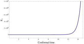
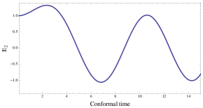
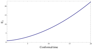
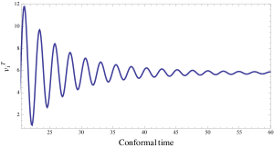
We confirm the general behaviour previously described with numerical plots given in Fig. 1, obtained solving the full equations of motion. In this figure we show the evolution of E1subscript𝐸1E_{1} and E2subscript𝐸2E_{2} as a function of conformal time (with arbitrary units) at early times during the radiation-dominated era for a given sub-horizon scale- we have set m2β1=102superscript𝑚2subscript𝛽1superscript102m^{2}\beta_{1}=10^{-2}, with the other β𝛽\betas vanishing, and arbitrary initial conditions of order 1 for both fields. For this plot and all the following numerical plots in this paper we will set Mg=1subscript𝑀𝑔1M_{g}=1. As we expected, E2subscript𝐸2E_{2} oscillates while E1subscript𝐸1E_{1} grows exponentially fast, increasing its value in many orders of magnitude, and eventually breaking the validity of linear perturbations. Note that large scales will not be affected by the exponential growth as much as small scales, as the former ones enter the horizon later, and therefore, experience the exponential expansion for a shorter period. Note also that in eq. (4.5), the exponential solution for E1subscript𝐸1E_{1} is due to the minus sign in the coefficient E1subscript𝐸1E_{1}, which when calculated for a general w𝑤w, will be negative for w>1/2𝑤12w>-1/2. Therefore, during the matter-dominated era, there will also be an exponential growth in E1subscript𝐸1E_{1}.

Refer to caption
Refer to caption
Figure 1: Evolution of E1subscript𝐸1E_{1} and E2subscript𝐸2E_{2} as a function of τ𝜏\tau for a given sub-horizon scales at early times during the radiation-dominated era. We have set β1m2=102subscript𝛽1superscript𝑚2superscript102\beta_{1}m^{2}=10^{-2} and the other β𝛽\betas vanishing.

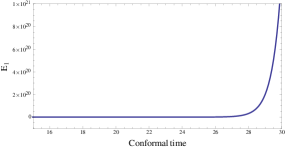
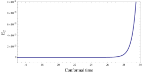
Furthermore, we can see that in eq. (4.4), we ignored the terms with E1subscript𝐸1E_{1} and E1superscriptsubscript𝐸1E_{1}^{\prime} to find the analytical solutions in eq. (4.6). However, as time goes on, E1subscript𝐸1E_{1} will grow many orders of magnitude and it will not be possible to discard the coupling between the two fields; E1subscript𝐸1E_{1} will feed back into the equation for E2subscript𝐸2E_{2}, making this latter field grow as well. Roughly, we expect that to happen when the terms for E1subscript𝐸1E_{1} are larger than those of E2subscript𝐸2E_{2} in eq. (4.4), i.e. when x7e15x/3N2much-less-thansuperscript𝑥7superscript𝑒15𝑥3superscript𝑁2x^{7}e^{-\sqrt{15}x/3}\ll N^{2}. Fig. 2 is a continuation of Fig. 1, as it shows the evolution at later times, where we can see the unstable behaviour in E2subscript𝐸2E_{2}.

We have studied the behaviour of scalar perturbations at early times during the radiation-dominated era, showing that generically, there is an exponential instability at early times in both scalar perturbations. During the matter era, the same instability appears. This exponential growth breaks the validity of first order perturbations and therefore we cannot trust the results. This instability could correspond to an actual physical problem of the model, or could be cured by higher order perturbations. A further analysis is needed to understand the nature of this instability and what it tells us, more generally, about the theory.
Refer to caption
Refer to caption
Figure 2: Evolution of E1subscript𝐸1E_{1} and E2subscript𝐸2E_{2} as a function of τ𝜏\tau in the radiation-dominated era for a given scale sub-horizon k𝑘k. At later times, both perturbation fields are growing exponentially fast, becoming several orders of magnitude larger than their early time value.

4.1.2 Late times

At late times, the background will approach a de-Sitter phase, where NN¯𝑁¯𝑁N\rightarrow\bar{N}, X1𝑋1X\rightarrow 1, Z~Z=Z¯~𝑍𝑍¯𝑍\tilde{Z}\rightarrow Z=\bar{Z}, and aH0𝑎subscript𝐻0\mathcal{H}\rightarrow aH_{0}, with N¯¯𝑁\bar{N}, Z¯¯𝑍\bar{Z} and H0subscript𝐻0H_{0} constants. Notice that the exact value of N¯¯𝑁\bar{N} depends on the parameters β𝛽\beta, and also

Z¯=β1+2β2N¯+β3N¯2,¯𝑍subscript𝛽12subscript𝛽2¯𝑁subscript𝛽3superscript¯𝑁2\displaystyle\bar{Z}=\beta_{1}+2\beta_{2}\bar{N}+\beta_{3}\bar{N}^{2},
H02=13m2N¯(β1+3β2N¯+3β3N¯2+β4N¯3),superscriptsubscript𝐻0213superscript𝑚2¯𝑁subscript𝛽13subscript𝛽2¯𝑁3subscript𝛽3superscript¯𝑁2subscript𝛽4superscript¯𝑁3\displaystyle H_{0}^{2}=\frac{1}{3}\frac{m^{2}}{\bar{N}}\left(\beta_{1}+3\beta_{2}\bar{N}+3\beta_{3}\bar{N}^{2}+\beta_{4}\bar{N}^{3}\right),
a=1H0τ,𝑎1subscript𝐻0𝜏\displaystyle a=\frac{1}{-H_{0}\tau}, (4.7)

where, in these coordinates, the infinite future is characterised by τ0𝜏0\tau\rightarrow 0.

We now study the evolution for super-horizon and sub-horizon scales in this de-Sitter phase, assuming w=0𝑤0w=0.

1. Super-horizon scales:

the evolution equations are now

E2′′+(2N¯2+1N¯2+1)E2(N¯2N¯2+1)E1+qN¯2(E2E1)=0,superscriptsubscript𝐸2′′2superscript¯𝑁21superscript¯𝑁21superscriptsubscript𝐸2superscript¯𝑁2superscript¯𝑁21superscriptsubscript𝐸1𝑞¯𝑁superscript2subscript𝐸2subscript𝐸10\displaystyle E_{2}^{\prime\prime}+\left(\frac{2\bar{N}^{2}+1}{\bar{N}^{2}+1}\right)\mathcal{H}E_{2}^{\prime}-\left(\frac{\bar{N}^{2}}{\bar{N}^{2}+1}\right)\mathcal{H}E_{1}^{\prime}+q\bar{N}\mathcal{H}^{2}(E_{2}-E_{1})=0,
E1′′+(N¯2+2N¯2+1)E1(1N¯2+1)E2+(qN¯)2(E1E2)=0,superscriptsubscript𝐸1′′superscript¯𝑁22superscript¯𝑁21superscriptsubscript𝐸11superscript¯𝑁21superscriptsubscript𝐸2𝑞¯𝑁superscript2subscript𝐸1subscript𝐸20\displaystyle E_{1}^{\prime\prime}+\left(\frac{\bar{N}^{2}+2}{\bar{N}^{2}+1}\right)\mathcal{H}E_{1}^{\prime}-\left(\frac{1}{\bar{N}^{2}+1}\right)\mathcal{H}E_{2}^{\prime}+\left(\frac{q}{\bar{N}}\right)\mathcal{H}^{2}(E_{1}-E_{2})=0, (4.8)

where qm2Z¯/H02𝑞superscript𝑚2¯𝑍superscriptsubscript𝐻02q\equiv m^{2}\bar{Z}/H_{0}^{2}. These equations are solved by:

E1=c0+c1τ2+c±τn±,subscript𝐸1subscript𝑐0subscript𝑐1superscript𝜏2subscript𝑐plus-or-minussuperscript𝜏subscript𝑛plus-or-minus\displaystyle E_{1}=c_{0}+c_{1}\tau^{2}+c_{\pm}\tau^{n_{\pm}}, (4.9)
E2=c0+c1τ2N¯2c±τn±,subscript𝐸2subscript𝑐0subscript𝑐1superscript𝜏2superscript¯𝑁2subscript𝑐plus-or-minussuperscript𝜏subscript𝑛plus-or-minus\displaystyle E_{2}=c_{0}+c_{1}\tau^{2}-\bar{N}^{2}c_{\pm}\tau^{n_{\pm}}, (4.10)

where c0subscript𝑐0c_{0}, c1subscript𝑐1c_{1} and c±subscript𝑐plus-or-minusc_{\pm} are some integration constants, and n±subscript𝑛plus-or-minusn_{\pm} is such that Re(n±)>0𝑅𝑒subscript𝑛plus-or-minus0Re(n_{\pm})>0. Therefore, both functions decay to the same constant.

2. Sub-horizon scales:

the evolution equations are now

E2′′+E294q[q(N¯2+1)2N¯]x4E1+12qN¯2(E2E1)=0,superscriptsubscript𝐸2′′superscriptsubscript𝐸294𝑞delimited-[]𝑞superscript¯𝑁212¯𝑁superscript𝑥4superscriptsubscript𝐸112𝑞¯𝑁superscript2subscript𝐸2subscript𝐸10\displaystyle E_{2}^{\prime\prime}+\mathcal{H}E_{2}^{\prime}-\frac{9}{4}\frac{q[q(\bar{N}^{2}+1)-2\bar{N}]}{x^{4}}\mathcal{H}E_{1}^{\prime}+\frac{1}{2}q\bar{N}\mathcal{H}^{2}(E_{2}-E_{1})=0,
E1′′+6E15E2+x22(E1E2)=0,superscriptsubscript𝐸1′′6superscriptsubscript𝐸15superscriptsubscript𝐸2superscript𝑥2superscript2subscript𝐸1subscript𝐸20\displaystyle E_{1}^{\prime\prime}+6\mathcal{H}E_{1}^{\prime}-5\mathcal{H}E_{2}^{\prime}+x^{2}\mathcal{H}^{2}(E_{1}-E_{2})=0, (4.11)

and when considering only the highest orders in x2superscript𝑥2x^{2}, the solutions are hypergeometric functions with power laws decaying to the same constant.

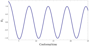
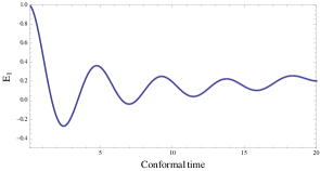
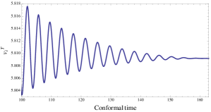
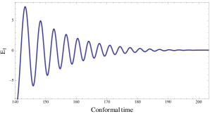
Figure 3 shows numerical results on the evolution of both scalar perturbations in the de-Sitter phase in the matter-dominated era for a given sub-horizon scale. As in previous plots, we considered m2β1=102superscript𝑚2subscript𝛽1superscript102m^{2}\beta_{1}=10^{-2} and the other β𝛽\betas vanishing, and arbitrary initial conditions of the same order for both fields. Here both fields are oscillating and approaching the same constant value.
Refer to caption
Refer to caption
Figure 3: Evolution of scalar perturbations as a function of the conformal time during the de-Sitter phase at late times in the matter-dominated era.

4.2 Bouncing branch

In this subsection we will show some approximate analytical solutions for the two physical scalar fields in the bouncing branch. First of all, note that the differences between the background evolutions in the expanding and bouncing branches occur only at early times, as at late times in both cases the metrics will enter a de-Sitter phase. Consequently, in the bouncing branch the evolution of perturbations at late times is the same as in the expanding branch. For this reason, in this subsection we focus on early times only. It is relevant in this case to show the evolution during the radiation-dominated era and the matter-dominated era, as fields do not evolve in the same way in both stages.

In this branch we can have different background solutions depending on the parameter values. We will distinguish the following cases: (a) β30subscript𝛽30\beta_{3}\not=0; (b) β3=0subscript𝛽30\beta_{3}=0 and (β43β2)0subscript𝛽43subscript𝛽20(\beta_{4}-3\beta_{2})\not=0; (c) β3=0subscript𝛽30\beta_{3}=0 and (β43β2)=0subscript𝛽43subscript𝛽20(\beta_{4}-3\beta_{2})=0; (d) β3=β2=0subscript𝛽3subscript𝛽20\beta_{3}=\beta_{2}=0. All the viable solutions with other combinations of null parameters are contained in these cases. As stated in [9], only case (d) is physically possible, as all the other cases have an exponential instability for sub-horizon scales at early times, similar to the one found in the expanding branch. For this reason, from now on we study perturbations for case (d) only. For more details about the other cases see Appendix A.3.

For case (d), notice that at early times N1much-greater-than𝑁1N\gg 1 and then eq. (3.12) approximates to:

ρ~=N2β4,~𝜌superscript𝑁2subscript𝛽4\tilde{\rho}=N^{2}\beta_{4}, (4.12)

and therefore we need to impose β4>0subscript𝛽40\beta_{4}>0. Conditions on the remaining parameters β0subscript𝛽0\beta_{0} and β1subscript𝛽1\beta_{1} are also present, as at late times the Friedmann equation (3.4) becomes:

2=a23m2(β0+3β1N¯),superscript2superscript𝑎23superscript𝑚2subscript𝛽03subscript𝛽1¯𝑁\mathcal{H}^{2}=\frac{a^{2}}{3}m^{2}\left(\beta_{0}+3\beta_{1}\bar{N}\right), (4.13)

where N¯¯𝑁\bar{N} is the late time value of the function N𝑁N. Consequently, we also need to impose β0+3β1N¯>0subscript𝛽03subscript𝛽1¯𝑁0\beta_{0}+3\beta_{1}\bar{N}>0. In general, we could satisfy this condition when both β𝛽\betas are positive or when one of them is negative (for some appropriate values). However, as we will see later, cases with β1<0subscript𝛽10\beta_{1}<0 bring instabilities in the solutions for scalars, vectors and tensor perturbations during the radiation-dominated era. Therefore, from now on we will assume β1>0subscript𝛽10\beta_{1}>0.

4.2.1 Early times radiation-dominated era

At early times N1much-greater-than𝑁1N\gg 1, and therefore we consider only leading order terms in N𝑁N in the equations of motion and we assume w=1/3𝑤13w=1/3. We again study the evolution in super-horizon and sub-horizon scales, focusing on case (d), where β3=β2=0subscript𝛽3subscript𝛽20\beta_{3}=\beta_{2}=0.

Super-horizon scales:

for super-horizon scales the equations become

E2′′+2E2+92x2Nβ1β4E113x22E2m2β1a2N2E1=0,superscriptsubscript𝐸2′′2superscriptsubscript𝐸292superscript𝑥2𝑁subscript𝛽1subscript𝛽4superscriptsubscript𝐸113superscript𝑥2superscript2subscript𝐸2superscript𝑚2subscript𝛽1superscript𝑎2𝑁2subscript𝐸10\displaystyle E_{2}^{\prime\prime}+2\mathcal{H}E_{2}^{\prime}+\frac{9}{2x^{2}}\frac{\mathcal{H}}{N}\frac{\beta_{1}}{\beta_{4}}E_{1}^{\prime}-\frac{1}{3}x^{2}\mathcal{H}^{2}E_{2}-\frac{m^{2}\beta_{1}a^{2}N}{2}E_{1}=0, (4.14)
E1′′+6β1β4N(E1x26E2)+x223E12m2β1a2Nx23E2=0superscriptsubscript𝐸1′′6subscript𝛽1subscript𝛽4𝑁superscriptsubscript𝐸1superscript𝑥26superscriptsubscript𝐸2superscript𝑥2superscript23subscript𝐸12superscript𝑚2subscript𝛽1superscript𝑎2𝑁superscript𝑥23subscript𝐸20\displaystyle E_{1}^{\prime\prime}+6\frac{\beta_{1}}{\beta_{4}}\frac{\mathcal{H}}{N}\left(E_{1}^{\prime}-\frac{x^{2}}{6}E_{2}^{\prime}\right)+\frac{x^{2}\mathcal{H}^{2}}{3}E_{1}-2m^{2}\beta_{1}a^{2}N\frac{x^{2}}{3}E_{2}=0 (4.15)

and when keeping only the lowest orders of x2superscript𝑥2x^{2} and the highest orders of N𝑁N, the solutions are E2=c1+c2/τsubscript𝐸2subscript𝑐1subscript𝑐2𝜏E_{2}=c_{1}+c_{2}/\tau and E1=c3+c4erf(pτ)subscript𝐸1subscript𝑐3subscript𝑐4erf𝑝𝜏E_{1}=c_{3}+c_{4}\mbox{erf}(p\tau), where c1subscript𝑐1c_{1}, c2subscript𝑐2c_{2}, c3subscript𝑐3c_{3} and c4subscript𝑐4c_{4} are some integration constants and p2=3β1/(β4N2τ2)=constsuperscript𝑝23subscript𝛽1subscript𝛽4superscript𝑁2superscript𝜏2𝑐𝑜𝑛𝑠𝑡p^{2}=3\beta_{1}/(\beta_{4}N^{2}\tau^{2})=const. Therefore, both functions decay to a constant in this regime.

Notice that if β1subscript𝛽1\beta_{1} were negative, the solution for E1subscript𝐸1E_{1} would be E1=c3+c4erf(i|p|τ)subscript𝐸1subscript𝑐3subscript𝑐4erf𝑖𝑝𝜏E_{1}=c_{3}+c_{4}\mbox{erf}(i|p|\tau), which would grow exponentially fast, breaking the linear perturbation approximation.

Sub-horizon scales:

the evolutions equations are now

E2′′+12x2E2+27x4Nβ1β4E1+13x22E23m2β1a2Nx2E1=0,superscriptsubscript𝐸2′′12superscript𝑥2superscriptsubscript𝐸227superscript𝑥4𝑁subscript𝛽1subscript𝛽4superscriptsubscript𝐸113superscript𝑥2superscript2subscript𝐸23superscript𝑚2subscript𝛽1superscript𝑎2𝑁superscript𝑥2subscript𝐸10\displaystyle E_{2}^{\prime\prime}+\frac{12}{x^{2}}\mathcal{H}E_{2}^{\prime}+\frac{27}{x^{4}}\frac{\mathcal{H}}{N}\frac{\beta_{1}}{\beta_{4}}E_{1}^{\prime}+\frac{1}{3}x^{2}\mathcal{H}^{2}E_{2}-\frac{3m^{2}\beta_{1}a^{2}N}{x^{2}}E_{1}=0, (4.16)
E1′′+6β1β4N(E1E2)+13x22E14m2β1a2NE2=0,superscriptsubscript𝐸1′′6subscript𝛽1subscript𝛽4𝑁superscriptsubscript𝐸1superscriptsubscript𝐸213superscript𝑥2superscript2subscript𝐸14superscript𝑚2subscript𝛽1superscript𝑎2𝑁subscript𝐸20\displaystyle E_{1}^{\prime\prime}+6\frac{\beta_{1}}{\beta_{4}}\frac{\mathcal{H}}{N}\left(E_{1}^{\prime}-E_{2}^{\prime}\right)+\frac{1}{3}x^{2}\mathcal{H}^{2}E_{1}-4m^{2}\beta_{1}a^{2}NE_{2}=0, (4.17)

and when keeping only the terms of order x2superscript𝑥2x^{2}, the solutions are Eie±ikτ/3proportional-tosubscript𝐸𝑖superscript𝑒plus-or-minus𝑖𝑘𝜏3E_{i}\propto e^{\pm ik\tau/\sqrt{3}}. Unlike in the expanding branch, in this case scalar perturbations are well behaved.

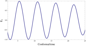
Fig. 4 shows numerical results for the evolution of scalar perturbations as a function of the conformal time (in arbitrary units), for a given sub-horizon scale during the radiation-dominated era at early times, confirming our previous analytical results. In this particular case we set m2β1=m2β4=102superscript𝑚2subscript𝛽1superscript𝑚2subscript𝛽4superscript102m^{2}\beta_{1}=m^{2}\beta_{4}=10^{-2}, and arbitrary initial conditions of order 1 for both fields.
Refer to caption
Refer to caption
Figure 4: Evolution of scalar perturbations as a function of τ𝜏\tau, during early times in the radiation-dominated for a given sub-horizon scales.

4.2.2 Early times matter-dominated era

As above, let us consider only leading terms in N𝑁N but now assume w=0𝑤0w=0.

Super-horizon scales:

the evolution equations are

E2′′+2E22Nβ1β4E113x22E2m2β1a2NE1=0,superscriptsubscript𝐸2′′2superscriptsubscript𝐸22𝑁subscript𝛽1subscript𝛽4superscriptsubscript𝐸113superscript𝑥2superscript2subscript𝐸2superscript𝑚2subscript𝛽1superscript𝑎2𝑁subscript𝐸10\displaystyle E_{2}^{\prime\prime}+2\mathcal{H}E_{2}^{\prime}-2\frac{\mathcal{H}}{N}\frac{\beta_{1}}{\beta_{4}}E_{1}^{\prime}-\frac{1}{3}x^{2}\mathcal{H}^{2}E_{2}-m^{2}\beta_{1}a^{2}NE_{1}=0, (4.18)
E1′′+52E1x23E2+56x22E113x22E2=0,superscriptsubscript𝐸1′′52superscriptsubscript𝐸1superscript𝑥23superscriptsubscript𝐸256superscript𝑥2superscript2subscript𝐸113superscript𝑥2superscript2subscript𝐸20\displaystyle E_{1}^{\prime\prime}+\frac{5}{2}\mathcal{H}E_{1}^{\prime}-\mathcal{H}\frac{x^{2}}{3}E_{2}^{\prime}+\frac{5}{6}x^{2}\mathcal{H}^{2}E_{1}-\frac{1}{3}x^{2}\mathcal{H}^{2}E_{2}=0, (4.19)

and when keeping only terms with the lowest orders in x2superscript𝑥2x^{2} (and highest powers in N𝑁N) we get: Ei=c1i+c2i/τnisubscript𝐸𝑖subscript𝑐1𝑖subscript𝑐2𝑖superscript𝜏subscript𝑛𝑖E_{i}=c_{1i}+c_{2i}/\tau^{n_{i}}, where c1isubscript𝑐1𝑖c_{1i} and c2isubscript𝑐2𝑖c_{2i} are some integration constants, and n1=4subscript𝑛14n_{1}=4 and n2=3subscript𝑛23n_{2}=3.

Sub-horizon scales

the evolution equations now reduce to

E2′′+E2+272x4Nβ1β4E1322E2m2β1a2N2E1=0,superscriptsubscript𝐸2′′superscriptsubscript𝐸2272superscript𝑥4𝑁subscript𝛽1subscript𝛽4superscriptsubscript𝐸132superscript2subscript𝐸2superscript𝑚2subscript𝛽1superscript𝑎2𝑁2subscript𝐸10\displaystyle E_{2}^{\prime\prime}+\mathcal{H}E_{2}^{\prime}+\frac{27}{2x^{4}}\frac{\mathcal{H}}{N}\frac{\beta_{1}}{\beta_{4}}E_{1}^{\prime}-\frac{3}{2}\mathcal{H}^{2}E_{2}-\frac{m^{2}\beta_{1}a^{2}N}{2}E_{1}=0, (4.20)
E1′′+32E112E2+122x2E12E2=0,superscriptsubscript𝐸1′′32superscriptsubscript𝐸112superscriptsubscript𝐸212superscript2superscript𝑥2subscript𝐸1superscript2subscript𝐸20\displaystyle E_{1}^{\prime\prime}+\frac{3}{2}\mathcal{H}E_{1}^{\prime}-\frac{1}{2}\mathcal{H}E_{2}^{\prime}+\frac{1}{2}\mathcal{H}^{2}x^{2}E_{1}-\mathcal{H}^{2}E_{2}=0, (4.21)

and when considering only the highest orders in x2superscript𝑥2x^{2} (and highest powers in N𝑁N) the solutions are E1e±ikτ/2proportional-tosubscript𝐸1superscript𝑒plus-or-minus𝑖𝑘𝜏2E_{1}\propto e^{\pm ik\tau/\sqrt{2}} and E2=c1/τ3+c2τ2subscript𝐸2subscript𝑐1superscript𝜏3subscript𝑐2superscript𝜏2E_{2}=c_{1}/\tau^{3}+c_{2}\tau^{2}, where c1subscript𝑐1c_{1} and c2subscript𝑐2c_{2} are some integration constants. Here we can see that E2subscript𝐸2E_{2} grows as a power law in time, which will affect E1subscript𝐸1E_{1} at later times, where this one will also start to grow as a power law.

Fig. 5 shows numerical solutions for both scalar fields for a given sub-horizon scale during early times in the matter-dominated era. In this case we set m2β1=m2β4=102superscript𝑚2subscript𝛽1superscript𝑚2subscript𝛽4superscript102m^{2}\beta_{1}=m^{2}\beta_{4}=10^{-2}, and arbitrary initial conditions of order one for both fields. As found in the analytical solutions, E1subscript𝐸1E_{1} oscillates while E2subscript𝐸2E_{2} grows as a power law.

Refer to caption
Refer to caption
Figure 5: Evolution of scalar perturbations as a function of τ𝜏\tau, during early times in the matter-dominated era for a given sub-horizon scale.

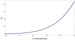
Analogous to the results for the expanding branch, in this case the quadratic growth in E2subscript𝐸2E_{2} will affect E1subscript𝐸1E_{1} at later times, making the latter field grow as a power law as well, as we observe in Fig. 6 (this figure is a continuation of Fig. 5).
Refer to caption
Refer to caption
Figure 6: Evolution of scalar perturbations during early times in the matter-dominated for a given sub-horizon scale.

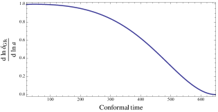
In addition, we can study the evolution of the gauge-invariant form for the density contrast δGIk=δρGI/ρ0subscript𝛿𝐺𝐼𝑘𝛿subscript𝜌𝐺𝐼subscript𝜌0\delta_{GIk}=\delta\rho_{GI}/\rho_{0},

δGIk=[δρ+ρ0(B2E2)]/ρ0,subscript𝛿𝐺𝐼𝑘delimited-[]𝛿𝜌superscriptsubscript𝜌0subscript𝐵2superscriptsubscript𝐸2subscript𝜌0\delta_{GIk}=[\delta\rho+\rho_{0}^{\prime}(B_{2}-E_{2}^{\prime})]/\rho_{0}, (4.22)

where δρ𝛿𝜌\delta\rho is given by the δT00\delta T^{0}{}_{0} in eq. (3.2). After fixing the gauge, and eliminating the auxiliary variables, δGIksubscript𝛿𝐺𝐼𝑘\delta_{GIk} can be expressed entirely in terms of Eisubscript𝐸𝑖E_{i} and Eisuperscriptsubscript𝐸𝑖E_{i}^{\prime} (see Appendix A.4). In Fig. 7 we see numerical results for the evolution of dlnδGIk/dlna𝑑subscript𝛿𝐺𝐼𝑘𝑑𝑎d\ln\delta_{GIk}/d\ln a as a function of the conformal time (in arbitrary units) for a given sub-horizon scale during the matter-dominated era. In this case we have also set m2β1=m2β4=104superscript𝑚2subscript𝛽1superscript𝑚2subscript𝛽4superscript104m^{2}\beta_{1}=m^{2}\beta_{4}=10^{-4}. We observe that at early times δGIksubscript𝛿𝐺𝐼𝑘\delta_{GIk} grows nearly proportional to the scale factor a𝑎a, and then it starts decaying faster as we enter into the de-Sitter phase, analogously to GR. A more detailed study on the comparison of this model with observations was done in [9].
Refer to caption
Figure 7: Evolution of density constrast as a function of the conformal time τ𝜏\tau in the matter-dominated era for a given sub-horizon scale.

It is important to remark that even though classical scalar fields do not evidence exponential instabilities in this branch, they do not satisfy the Higuchi bound (see Appendix B for details), and therefore one scalar field propagates as a ghost, i.e. with a negative kinetic term. Consequently, instabilities might appear when studying higher order perturbations, and negative norm states would appear when quantising the linear theory massive gravity (see [40]).

5 Vector perturbations

Analogously to the previous section, we now study the evolution of vector perturbations in different regimes, by making relevant approximations to the full equations of motion given by eq. (3.3)-(3.3).

5.1 Expanding branch

Recall that the expanding branch is characterised by N1much-less-than𝑁1N\ll 1 at early times and a de-Sitter phase at late times.

5.1.1 Early times radiation-dominated era

Considering w=1/3𝑤13w=1/3 and leading order terms in 1/N1𝑁1/N, the equations for vector perturbations become:

F2i′′+2(4x4+33x2+40)(8+x2)(x2+5)F2i16(3x2+20)(8+x2)(x2+5)viT+3(x2+5)2F2i=0,superscriptsubscript𝐹2𝑖′′24superscript𝑥433superscript𝑥2408superscript𝑥2superscript𝑥25superscriptsubscript𝐹2𝑖163superscript𝑥2208superscript𝑥2superscript𝑥25subscriptsuperscript𝑣𝑇𝑖3superscript𝑥25superscript2subscript𝐹2𝑖0\displaystyle F_{2i}^{\prime\prime}+\frac{2(4x^{4}+33x^{2}+40)\mathcal{H}}{(8+x^{2})(x^{2}+5)}F_{2i}^{\prime}-\frac{16(3x^{2}+20)\mathcal{H}}{(8+x^{2})(x^{2}+5)}v^{T}_{i}+3(x^{2}+5)\mathcal{H}^{2}F_{2i}=0, (5.1)
viT+8(8x2+50)(8+x2)(x2+5)viT2(4x2+25)x2(8+x2)(x2+5)F2i3(x2+5)2F2i=0,subscriptsuperscript𝑣superscript𝑇𝑖88superscript𝑥2508superscript𝑥2superscript𝑥25subscriptsuperscript𝑣𝑇𝑖24superscript𝑥225superscript𝑥28superscript𝑥2superscript𝑥25superscriptsubscript𝐹2𝑖3superscript𝑥25superscript2subscript𝐹2𝑖0\displaystyle v^{T^{\prime}}_{i}+\frac{8(8x^{2}+50)\mathcal{H}}{(8+x^{2})(x^{2}+5)}v^{T}_{i}-\frac{2(4x^{2}+25)\mathcal{H}x^{2}}{(8+x^{2})(x^{2}+5)}F_{2i}^{\prime}-3(x^{2}+5)\mathcal{H}^{2}F_{2i}=0, (5.2)

where x=k/𝑥𝑘x=k/\mathcal{H}.

Super-horizon scales:

the evolution equations reduce to

F2i′′+2F2i8viT+152F2i=0,subscriptsuperscript𝐹′′2𝑖2subscriptsuperscript𝐹2𝑖8subscriptsuperscript𝑣𝑇𝑖15superscript2subscript𝐹2𝑖0\displaystyle F^{\prime\prime}_{2i}+2\mathcal{H}F^{\prime}_{2i}-8\mathcal{H}v^{T}_{i}+15\mathcal{H}^{2}F_{2i}=0, (5.3)
viT+10viT54x2F2i152F2i=0,subscriptsuperscript𝑣superscript𝑇𝑖10subscriptsuperscript𝑣𝑇𝑖54superscript𝑥2subscriptsuperscript𝐹2𝑖15superscript2subscript𝐹2𝑖0\displaystyle v^{T^{\prime}}_{i}+10\mathcal{H}v^{T}_{i}-\frac{5}{4}x^{2}\mathcal{H}F^{\prime}_{2i}-15\mathcal{H}^{2}F_{2i}=0, (5.4)

and, ignoring terms of order x2superscript𝑥2x^{2}, the solutions are F2i=c1/τ+c±τn±subscript𝐹2𝑖subscript𝑐1𝜏subscript𝑐plus-or-minussuperscript𝜏subscript𝑛plus-or-minusF_{2i}=c_{1}/\tau+c_{\pm}\tau^{n_{\pm}} and viT=c2/τ2+b±τn±subscriptsuperscript𝑣𝑇𝑖subscript𝑐2superscript𝜏2subscript𝑏plus-or-minussuperscript𝜏subscript𝑛plus-or-minusv^{T}_{i}=c_{2}/\tau^{2}+b_{\pm}\tau^{n_{\pm}}, where n±<0limit-from𝑛plus-or-minus0n\pm<0, and where c1subscript𝑐1c_{1}, c2subscript𝑐2c_{2}, c±subscript𝑐plus-or-minusc_{\pm} and b±subscript𝑏plus-or-minusb_{\pm} are some integration constants related to each other. Therefore, both vector perturbations decay to zero in this regime.

Sub-horizon scales:

the evolution equations reduce to

F2i′′+8F2i48x2viT+3x22F2i=0,subscriptsuperscript𝐹′′2𝑖8subscriptsuperscript𝐹2𝑖48superscript𝑥2subscriptsuperscript𝑣𝑇𝑖3superscript𝑥2superscript2subscript𝐹2𝑖0\displaystyle F^{\prime\prime}_{2i}+8\mathcal{H}F^{\prime}_{2i}-\frac{48}{x^{2}}\mathcal{H}v^{T}_{i}+3x^{2}\mathcal{H}^{2}F_{2i}=0, (5.5)
viT+64x2viT8F2i3x22F2i=0,subscriptsuperscript𝑣superscript𝑇𝑖64superscript𝑥2subscriptsuperscript𝑣𝑇𝑖8subscriptsuperscript𝐹2𝑖3superscript𝑥2superscript2subscript𝐹2𝑖0\displaystyle v^{T^{\prime}}_{i}+\frac{64}{x^{2}}\mathcal{H}v^{T}_{i}-8\mathcal{H}F^{\prime}_{2i}-3x^{2}\mathcal{H}^{2}F_{2i}=0, (5.6)

and when ignoring terms of order x2superscript𝑥2x^{-2}, the solutions are

F2ie±ik3τ/τ4,proportional-tosubscript𝐹2𝑖superscript𝑒plus-or-minus𝑖𝑘3𝜏superscript𝜏4\displaystyle F_{2i}\propto e^{\pm ik\sqrt{3}\tau}/\tau^{4}, (5.7)
viT=c1c±e±ik3τ/τ4,subscriptsuperscript𝑣𝑇𝑖subscript𝑐1subscript𝑐plus-or-minussuperscript𝑒plus-or-minus𝑖𝑘3𝜏superscript𝜏4\displaystyle v^{T}_{i}=c_{1}-c_{\pm}e^{\pm ik\sqrt{3}\tau}/\tau^{4}, (5.8)

where c1subscript𝑐1c_{1} and c±subscript𝑐plus-or-minusc_{\pm} are come integration constants related to those of F2isubscript𝐹2𝑖F_{2i}. Therefore, in this regime both functions decay as a4superscript𝑎4a^{4}.

Figure 8 shows numerical results for the evolution of vector perturbations as a function of τ𝜏\tau, during early times in the radiation-dominated era for a given sub-horizon scale; we have set m2β1=102superscript𝑚2subscript𝛽1superscript102m^{2}\beta_{1}=10^{-2} while all other β𝛽\betas are vanishing, and we have chosen arbitrary initial conditions of the same order for both fields. We can clearly see that both fields decay in the same way, but while F2isubscript𝐹2𝑖F_{2i} is oscillating around 0, viTsubscriptsuperscript𝑣𝑇𝑖v^{T}_{i} oscillates around a constant value. We find similar behaviour the matter-dominated era.
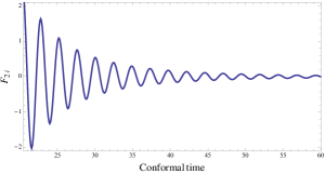
Refer to caption
Refer to caption
Figure 8: Evolution of vector perturbations as a function of τ𝜏\tau, during early times in the radiation-dominated era for a given sub-horizon scale.

5.1.2 Late times

We now assume w=0𝑤0w=0 and a de-Sitter space-time where N𝑁N takes the constant value N¯¯𝑁\bar{N}, and a1/τproportional-to𝑎1𝜏a\propto 1/\tau, with τ0𝜏0\tau\rightarrow 0 being the infinite future.

Super-horizon scales:

the evolution equations are

F2i′′+2F2i+a2x2F2i=0,x2=m2Z¯(N¯2+1)/N¯,formulae-sequencesuperscriptsubscript𝐹2𝑖′′2superscriptsubscript𝐹2𝑖superscript𝑎2subscript𝑥2subscript𝐹2𝑖0subscript𝑥2superscript𝑚2¯𝑍superscript¯𝑁21¯𝑁\displaystyle F_{2i}^{\prime\prime}+2\mathcal{H}F_{2i}^{\prime}+a^{2}x_{2}F_{2i}=0,\;x_{2}=m^{2}\bar{Z}(\bar{N}^{2}+1)/\bar{N}, (5.9)
viT+viT1N¯2+1F2ia2x1F2i=0,x1=m2Z¯/N¯,formulae-sequencesubscriptsuperscript𝑣superscript𝑇𝑖subscriptsuperscript𝑣𝑇𝑖1superscript¯𝑁21superscriptsubscript𝐹2𝑖superscript𝑎2subscript𝑥1subscript𝐹2𝑖0subscript𝑥1superscript𝑚2¯𝑍¯𝑁\displaystyle v^{T^{\prime}}_{i}+\mathcal{H}v^{T}_{i}-\frac{1}{\bar{N}^{2}+1}\mathcal{H}F_{2i}^{\prime}-a^{2}x_{1}F_{2i}=0,\;x_{1}=m^{2}\bar{Z}/\bar{N}, (5.10)

and are solved by F2iτn±proportional-tosubscript𝐹2𝑖superscript𝜏subscript𝑛plus-or-minusF_{2i}\propto\tau^{n_{\pm}} and viT=c1τ+c±τn±1subscriptsuperscript𝑣𝑇𝑖subscript𝑐1𝜏subscript𝑐plus-or-minussuperscript𝜏limit-from𝑛plus-or-minus1v^{T}_{i}=c_{1}\tau+c_{\pm}\tau^{n\pm-1}; Re(n±)>1𝑅𝑒subscript𝑛plus-or-minus1Re(n_{\pm})>1, while c1subscript𝑐1c_{1} and c±subscript𝑐plus-or-minusc_{\pm} are integration constants related to those of F2isubscript𝐹2𝑖F_{2i}.

Sub-horizon scales:

the evolution equations reduce to

F2i′′+4F2i+x22F2i=0,superscriptsubscript𝐹2𝑖′′4superscriptsubscript𝐹2𝑖superscript𝑥2superscript2subscript𝐹2𝑖0\displaystyle F_{2i}^{\prime\prime}+4\mathcal{H}F_{2i}^{\prime}+x^{2}\mathcal{H}^{2}F_{2i}=0, (5.11)
viT+viT3F2ix22F2i=0,subscriptsuperscript𝑣superscript𝑇𝑖subscriptsuperscript𝑣𝑇𝑖3superscriptsubscript𝐹2𝑖superscript𝑥2superscript2subscript𝐹2𝑖0\displaystyle v^{T^{\prime}}_{i}+\mathcal{H}v^{T}_{i}-3\mathcal{H}F_{2i}^{\prime}-x^{2}\mathcal{H}^{2}F_{2i}=0, (5.12)

and are solved by F2iτ2e±ikτproportional-tosubscript𝐹2𝑖superscript𝜏2superscript𝑒plus-or-minus𝑖𝑘𝜏F_{2i}\propto\tau^{2}e^{\pm ik\tau} and viT=c1τ+c±τ2e±ikτsubscriptsuperscript𝑣𝑇𝑖subscript𝑐1𝜏subscript𝑐plus-or-minussuperscript𝜏2superscript𝑒plus-or-minus𝑖𝑘𝜏v^{T}_{i}=c_{1}\tau+c_{\pm}\tau^{2}e^{\pm ik\tau}, where c1subscript𝑐1c_{1} and c±subscript𝑐plus-or-minusc_{\pm} are integration constants related to those of F2isubscript𝐹2𝑖F_{2i}. In this case, both perturbations are decaying.

Figure 9 shows numerical solutions for the evolution of vector perturbations as a function of τ𝜏\tau, during late times for a given sub-horizon scale. Again, we have set m2β1=102superscript𝑚2subscript𝛽1superscript102m^{2}\beta_{1}=10^{-2} and all other β𝛽\betas vanishing, and arbitrary initial conditions of the same order for both fields. Both fields oscillate and decay in the same way, but while F2isubscript𝐹2𝑖F_{2i} is oscillating around 0, viTsubscriptsuperscript𝑣𝑇𝑖v^{T}_{i} oscillates around a decaying function.
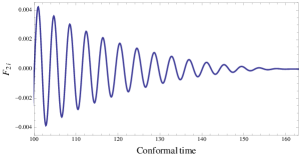
Refer to caption
Refer to caption
Figure 9: Evolution of vector perturbations during late times in the de-Sitter phase for a sub-horizon scale.

5.2 Bouncing branch

As we have mentioned before, the bouncing branch is characterised by N1much-greater-than𝑁1N\gg 1 at early times and a de-Sitter phase at late times. Next, we study the evolution of vector perturbations at early times in the same way we previously did for scalar perturbations.

5.2.1 Early times radiation-dominated era

We will start by assuming w=1/3𝑤13w=1/3. When considering only leading terms in N𝑁N, the equations of motion become:

F2i′′+20(x2+10)F2i+16x2+10viT+3β12β42N(2+x2)F2i=0,superscriptsubscript𝐹2𝑖′′20superscript𝑥210superscriptsubscript𝐹2𝑖16superscript𝑥210subscriptsuperscript𝑣𝑇𝑖3subscript𝛽12subscript𝛽4superscript2𝑁2superscript𝑥2subscript𝐹2𝑖0\displaystyle F_{2i}^{\prime\prime}+\frac{20\mathcal{H}}{(x^{2}+10)}F_{2i}^{\prime}+\frac{16\mathcal{H}}{x^{2}+10}v^{T}_{i}+\frac{3\beta_{1}}{2\beta_{4}}\frac{\mathcal{H}^{2}}{N}(2+x^{2})F_{2i}=0, (5.13)
viT+83N(9β124β0β4)β1β4(x2+10)viTx23N(9β124β0β4)β1β4(x2+10)F2i3β12β4x22NF2i=0.superscriptsubscript𝑣𝑖superscript𝑇83𝑁9superscriptsubscript𝛽124subscript𝛽0subscript𝛽4subscript𝛽1subscript𝛽4superscript𝑥210subscriptsuperscript𝑣𝑇𝑖superscript𝑥23𝑁9superscriptsubscript𝛽124subscript𝛽0subscript𝛽4subscript𝛽1subscript𝛽4superscript𝑥210superscriptsubscript𝐹2𝑖3subscript𝛽12subscript𝛽4superscript𝑥2superscript2𝑁subscript𝐹2𝑖0\displaystyle v_{i}^{T^{\prime}}+\frac{8}{3}\frac{\mathcal{H}}{N}\frac{(9\beta_{1}^{2}-4\beta_{0}\beta_{4})}{\beta_{1}\beta_{4}(x^{2}+10)}v^{T}_{i}-\frac{x^{2}}{3}\frac{\mathcal{H}}{N}\frac{(9\beta_{1}^{2}-4\beta_{0}\beta_{4})}{\beta_{1}\beta_{4}(x^{2}+10)}F_{2i}^{\prime}-\frac{3\beta_{1}}{2\beta_{4}}\frac{x^{2}\mathcal{H}^{2}}{N}F_{2i}=0. (5.14)

We now study these equations for sub-horizon and super-horizon scales.

Super-horizon scales:

the evolution equations reduce to

F2i′′+2F2i+85viT+3β1β42NF2i=0,superscriptsubscript𝐹2𝑖′′2superscriptsubscript𝐹2𝑖85subscriptsuperscript𝑣𝑇𝑖3subscript𝛽1subscript𝛽4superscript2𝑁subscript𝐹2𝑖0\displaystyle F_{2i}^{\prime\prime}+2\mathcal{H}F_{2i}^{\prime}+\frac{8}{5}\mathcal{H}v^{T}_{i}+\frac{3\beta_{1}}{\beta_{4}}\frac{\mathcal{H}^{2}}{N}F_{2i}=0, (5.15)
viT+415N(9β124β0β4)β1β4viTx230N(9β124β0β4)β1β4F2i3β12β4x22NF2i=0.superscriptsubscript𝑣𝑖superscript𝑇415𝑁9superscriptsubscript𝛽124subscript𝛽0subscript𝛽4subscript𝛽1subscript𝛽4subscriptsuperscript𝑣𝑇𝑖superscript𝑥230𝑁9superscriptsubscript𝛽124subscript𝛽0subscript𝛽4subscript𝛽1subscript𝛽4superscriptsubscript𝐹2𝑖3subscript𝛽12subscript𝛽4superscript𝑥2superscript2𝑁subscript𝐹2𝑖0\displaystyle v_{i}^{T^{\prime}}+\frac{4}{15}\frac{\mathcal{H}}{N}\frac{(9\beta_{1}^{2}-4\beta_{0}\beta_{4})}{\beta_{1}\beta_{4}}v^{T}_{i}-\frac{x^{2}}{30}\frac{\mathcal{H}}{N}\frac{(9\beta_{1}^{2}-4\beta_{0}\beta_{4})}{\beta_{1}\beta_{4}}F_{2i}^{\prime}-\frac{3\beta_{1}}{2\beta_{4}}\frac{x^{2}\mathcal{H}^{2}}{N}F_{2i}=0. (5.16)

Ignoring terms of order x2superscript𝑥2x^{2} and lowest order terms of N𝑁N, the solutions are F2i=c1+c2/τsubscript𝐹2𝑖subscript𝑐1subscript𝑐2𝜏F_{2i}=c_{1}+c_{2}/\tau and viTep2τ2proportional-tosubscriptsuperscript𝑣𝑇𝑖superscript𝑒superscript𝑝2superscript𝜏2v^{T}_{i}\propto e^{-p^{2}\tau^{2}}, where c1subscript𝑐1c_{1} and c2subscript𝑐2c_{2} are some integration constants, and p2=2(9β124β0β4)/(15β1β4Nτ2)=constsuperscript𝑝229superscriptsubscript𝛽124subscript𝛽0subscript𝛽415subscript𝛽1subscript𝛽4𝑁superscript𝜏2𝑐𝑜𝑛𝑠𝑡p^{2}=2(9\beta_{1}^{2}-4\beta_{0}\beta_{4})/(15\beta_{1}\beta_{4}N\tau^{2})=const. Notice that here we have assumed that (9β124β0β4)/(β1β4)>09superscriptsubscript𝛽124subscript𝛽0subscript𝛽4subscript𝛽1subscript𝛽40(9\beta_{1}^{2}-4\beta_{0}\beta_{4})/(\beta_{1}\beta_{4})>0, since otherwise viTsuperscript𝑣𝑖𝑇v^{iT} would grow exponentially fast, creating an instability in the solutions.

Sub-horizon scales:

the evolution equations reduce to

F2i′′+20x2F2i+16x2viT+3β12β42x2NF2i=0,superscriptsubscript𝐹2𝑖′′20superscript𝑥2superscriptsubscript𝐹2𝑖16superscript𝑥2subscriptsuperscript𝑣𝑇𝑖3subscript𝛽12subscript𝛽4superscript2superscript𝑥2𝑁subscript𝐹2𝑖0\displaystyle F_{2i}^{\prime\prime}+\frac{20}{x^{2}}\mathcal{H}F_{2i}^{\prime}+\frac{16\mathcal{H}}{x^{2}}v^{T}_{i}+\frac{3\beta_{1}}{2\beta_{4}}\frac{\mathcal{H}^{2}x^{2}}{N}F_{2i}=0, (5.17)
viT+83N(9β124β0β4)β1β4x2viT13N(9β124β0β4)β1β4F2i3β12β4x22NF2i=0.superscriptsubscript𝑣𝑖superscript𝑇83𝑁9superscriptsubscript𝛽124subscript𝛽0subscript𝛽4subscript𝛽1subscript𝛽4superscript𝑥2subscriptsuperscript𝑣𝑇𝑖13𝑁9superscriptsubscript𝛽124subscript𝛽0subscript𝛽4subscript𝛽1subscript𝛽4superscriptsubscript𝐹2𝑖3subscript𝛽12subscript𝛽4superscript𝑥2superscript2𝑁subscript𝐹2𝑖0\displaystyle v_{i}^{T^{\prime}}+\frac{8}{3}\frac{\mathcal{H}}{N}\frac{(9\beta_{1}^{2}-4\beta_{0}\beta_{4})}{\beta_{1}\beta_{4}x^{2}}v^{T}_{i}-\frac{1}{3}\frac{\mathcal{H}}{N}\frac{(9\beta_{1}^{2}-4\beta_{0}\beta_{4})}{\beta_{1}\beta_{4}}F_{2i}^{\prime}-\frac{3\beta_{1}}{2\beta_{4}}\frac{x^{2}\mathcal{H}^{2}}{N}F_{2i}=0. (5.18)

Considering only highest order terms in x2superscript𝑥2x^{2}, the solutions are F2ie±iKτ2/2/τproportional-tosubscript𝐹2𝑖superscript𝑒plus-or-minus𝑖𝐾superscript𝜏22𝜏F_{2i}\propto e^{\pm iK\tau^{2}/2}/\sqrt{\tau} and viTe±iKτ2/2τproportional-tosubscriptsuperscript𝑣𝑇𝑖superscript𝑒plus-or-minus𝑖𝐾superscript𝜏22𝜏v^{T}_{i}\propto e^{\pm iK\tau^{2}/2}\sqrt{\tau}, where K2=3β12β4k2Nτ2superscript𝐾23subscript𝛽12subscript𝛽4superscript𝑘2𝑁superscript𝜏2K^{2}=\frac{3\beta_{1}}{2\beta_{4}}\frac{k^{2}}{N\tau^{2}}. We then see that, contrary to GR, F2isubscript𝐹2𝑖F_{2i} decays but the vorticity field viTsubscriptsuperscript𝑣𝑇𝑖v^{T}_{i} grows. This modification happens as the dominant term in eq. (5.18) corresponds to the interaction term with F2isubscript𝐹2𝑖F_{2i} instead of the term with viTsubscriptsuperscript𝑣𝑇𝑖v^{T}_{i}.

Notice that if β1subscript𝛽1\beta_{1} were negative, solutions for F2isubscript𝐹2𝑖F_{2i} and viTsuperscript𝑣𝑖𝑇v^{iT} would be combinations of Bessel I and K functions, which would grow exponentially fast, creating an instability in the solutions.

Figure 10 shows numerical results for the evolution of vector perturbations as a function of τ𝜏\tau, during early times for a given sub-horizon scale in the radiation-dominated era. In this case we have set m2β1=m2β4=102superscript𝑚2subscript𝛽1superscript𝑚2subscript𝛽4superscript102m^{2}\beta_{1}=m^{2}\beta_{4}=10^{-2}, and arbitrary initial conditions of the same order for both fields. As expected due to the analytical solutions, F2isubscript𝐹2𝑖F_{2i} decays in time while viTsubscriptsuperscript𝑣𝑇𝑖v^{T}_{i} grows.

Refer to caption
Refer to caption
Figure 10: Evolution of vector perturbations as a function of τ𝜏\tau, during early times in the radiation-dominated era for a sub-horizon scale.

5.2.2 Early times matter-dominated era

Let us now assume that w=0𝑤0w=0, and consider only leading order terms in N𝑁N in the equations of motion to find

F2i′′+(5x2+24)2(x2+6)F2i3x2+6viT+14x22F2i=0,superscriptsubscript𝐹2𝑖′′5superscript𝑥2242superscript𝑥26superscriptsubscript𝐹2𝑖3superscript𝑥26subscriptsuperscript𝑣𝑇𝑖14superscript𝑥2superscript2subscript𝐹2𝑖0\displaystyle F_{2i}^{\prime\prime}+\mathcal{H}\frac{(5x^{2}+24)}{2(x^{2}+6)}F_{2i}^{\prime}-\frac{3\mathcal{H}}{x^{2}+6}v^{T}_{i}+\frac{1}{4}x^{2}\mathcal{H}^{2}F_{2i}=0, (5.19)
viT+(x2+15)(x2+6)viT32x2(x2+6)F2i14x22F2i=0.superscriptsubscript𝑣𝑖superscript𝑇superscript𝑥215superscript𝑥26subscriptsuperscript𝑣𝑇𝑖32superscript𝑥2superscript𝑥26superscriptsubscript𝐹2𝑖14superscript𝑥2superscript2subscript𝐹2𝑖0\displaystyle v_{i}^{T^{\prime}}+\mathcal{H}\frac{(x^{2}+15)}{(x^{2}+6)}v^{T}_{i}-\frac{3}{2}\mathcal{H}\frac{x^{2}}{(x^{2}+6)}F_{2i}^{\prime}-\frac{1}{4}x^{2}\mathcal{H}^{2}F_{2i}=0. (5.20)
Super-horizon scales:

the evolution equations become

F2i′′+2F2i12viT+14x22F2i=0,superscriptsubscript𝐹2𝑖′′2superscriptsubscript𝐹2𝑖12subscriptsuperscript𝑣𝑇𝑖14superscript𝑥2superscript2subscript𝐹2𝑖0\displaystyle F_{2i}^{\prime\prime}+2\mathcal{H}F_{2i}^{\prime}-\frac{1}{2}\mathcal{H}v^{T}_{i}+\frac{1}{4}x^{2}\mathcal{H}^{2}F_{2i}=0, (5.21)
viT+156viT14x2F2i14x22F2i=0,superscriptsubscript𝑣𝑖superscript𝑇156subscriptsuperscript𝑣𝑇𝑖14superscript𝑥2superscriptsubscript𝐹2𝑖14superscript𝑥2superscript2subscript𝐹2𝑖0\displaystyle v_{i}^{T^{\prime}}+\frac{15}{6}\mathcal{H}v^{T}_{i}-\frac{1}{4}\mathcal{H}x^{2}F_{2i}^{\prime}-\frac{1}{4}x^{2}\mathcal{H}^{2}F_{2i}=0, (5.22)

and, when ignoring terms of order x2superscript𝑥2x^{2}, the solutions are F2i=c1/τ4+c2/τ3+c3subscript𝐹2𝑖subscript𝑐1superscript𝜏4subscript𝑐2superscript𝜏3subscript𝑐3F_{2i}=c_{1}/\tau^{4}+c_{2}/\tau^{3}+c_{3} and viT1/τ5proportional-tosubscriptsuperscript𝑣𝑇𝑖1superscript𝜏5v^{T}_{i}\propto 1/\tau^{5}, where c1subscript𝑐1c_{1}, c2subscript𝑐2c_{2} and c3subscript𝑐3c_{3} are some integration constants. Therefore, both functions decay in time.

Sub-horizon scales

the evolution equations now reduce to

F2i′′+52F2i3x2viT+14x22F2i=0,superscriptsubscript𝐹2𝑖′′52superscriptsubscript𝐹2𝑖3superscript𝑥2subscriptsuperscript𝑣𝑇𝑖14superscript𝑥2superscript2subscript𝐹2𝑖0\displaystyle F_{2i}^{\prime\prime}+\frac{5}{2}\mathcal{H}F_{2i}^{\prime}-\frac{3\mathcal{H}}{x^{2}}v^{T}_{i}+\frac{1}{4}x^{2}\mathcal{H}^{2}F_{2i}=0, (5.23)
viT+viT32F2i14x22F2i=0,superscriptsubscript𝑣𝑖superscript𝑇subscriptsuperscript𝑣𝑇𝑖32superscriptsubscript𝐹2𝑖14superscript𝑥2superscript2subscript𝐹2𝑖0\displaystyle v_{i}^{T^{\prime}}+\mathcal{H}v^{T}_{i}-\frac{3}{2}\mathcal{H}F_{2i}^{\prime}-\frac{1}{4}x^{2}\mathcal{H}^{2}F_{2i}=0, (5.24)

and, when ignoring terms of order x2superscript𝑥2x^{-2}, the solutions are F2ie±ikτ/2/τ3/2proportional-tosubscript𝐹2𝑖superscript𝑒plus-or-minus𝑖𝑘𝜏2superscript𝜏32F_{2i}\propto e^{\pm ik\tau/2}/\tau^{3/2} and viT=c1/τ2+c±e±ikτ/2/τ3/2subscriptsuperscript𝑣𝑇𝑖subscript𝑐1superscript𝜏2subscript𝑐plus-or-minussuperscript𝑒plus-or-minus𝑖𝑘𝜏2superscript𝜏32v^{T}_{i}=c_{1}/\tau^{2}+c_{\pm}e^{\pm ik\tau/2}/\tau^{3/2}, where c1subscript𝑐1c_{1} and c±subscript𝑐plus-or-minusc_{\pm} are integration constants.

Figure 11 shows numerical results for the evolution of vector perturbations as a function of τ𝜏\tau, during early times for a given sub-horizon scale in the matter-dominated era. In this case we have set m2β1=m2β4=102superscript𝑚2subscript𝛽1superscript𝑚2subscript𝛽4superscript102m^{2}\beta_{1}=m^{2}\beta_{4}=10^{-2}, and arbitrary initial conditions of the same order for both fields. With these plots we confirm our analytical results.
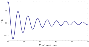
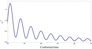
Refer to caption
Refer to caption
Figure 11: Evolution of vector perturbations as a function of τ𝜏\tau, during early times in matter-dominated era for a given sub-horizon scale.

6 Tensor perturbations

In this section we find approximate analytical solutions for the tensor modes in the relevant regimes for both branches. As mentioned previously, in the bouncing branch, we restrict our study of the tensor modes for the case β3=β2=0subscript𝛽3subscript𝛽20\beta_{3}=\beta_{2}=0.

6.1 Expanding branch

As before, we study the solutions of tensor perturbations at early and late times.

6.1.1 Early times

Let us consider only leading order terms in 1/N1𝑁1/N, as N1much-less-than𝑁1N\ll 1 at early times in this branch. In this approximation eq. (3.49)-(3.50) become:

h2p′′+2h2p+x22h2p+m2a2Nβ1(h2ph1p)=0,superscriptsubscript2𝑝′′2superscriptsubscript2𝑝superscript𝑥2superscript2subscript2𝑝superscript𝑚2superscript𝑎2𝑁subscript𝛽1subscript2𝑝subscript1𝑝0\displaystyle h_{2p}^{\prime\prime}+2\mathcal{H}h_{2p}^{\prime}+x^{2}\mathcal{H}^{2}h_{2p}+m^{2}a^{2}N\beta_{1}(h_{2p}-h_{1p})=0, (6.1)
h1p′′+2(4+3w)h1p+(4+3w)2x22h1p+3(4+3w)2(h1ph2p)=0.superscriptsubscript1𝑝′′243𝑤superscriptsubscript1𝑝superscript43𝑤2superscript𝑥2superscript2subscript1𝑝343𝑤superscript2subscript1𝑝subscript2𝑝0\displaystyle h_{1p}^{\prime\prime}+2(4+3w)\mathcal{H}h_{1p}^{\prime}+(4+3w)^{2}x^{2}\mathcal{H}^{2}h_{1p}+3(4+3w)\mathcal{H}^{2}(h_{1p}-h_{2p})=0. (6.2)
Super-horizon scales:

the equations simplify to the form

h2p′′+2h2p=0,superscriptsubscript2𝑝′′2superscriptsubscript2𝑝0\displaystyle h_{2p}^{\prime\prime}+2\mathcal{H}h_{2p}^{\prime}=0, (6.3)
h1p′′+10h1p+152(h1ph2p)=0,superscriptsubscript1𝑝′′10superscriptsubscript1𝑝15superscript2subscript1𝑝subscript2𝑝0\displaystyle h_{1p}^{\prime\prime}+10\mathcal{H}h_{1p}^{\prime}+15\mathcal{H}^{2}(h_{1p}-h_{2p})=0, (6.4)

and are solved by h2p=c1+c2/τsubscript2𝑝subscript𝑐1subscript𝑐2𝜏h_{2p}=c_{1}+c_{2}/\tau and h1p=c3+c4/τ+c±τn±subscript1𝑝subscript𝑐3subscript𝑐4𝜏subscript𝑐plus-or-minussuperscript𝜏subscript𝑛plus-or-minush_{1p}=c_{3}+c_{4}/\tau+c_{\pm}\tau^{n_{\pm}}, with n±=(9±21)/2<0subscript𝑛plus-or-minusplus-or-minus92120n_{\pm}=-(9\pm\sqrt{21})/2<0, where c1subscript𝑐1c_{1}, c2subscript𝑐2c_{2}, c3subscript𝑐3c_{3}, c4subscript𝑐4c_{4} and c±subscript𝑐plus-or-minusc_{\pm} are integrations constants, related to each other. Therefore, both solutions decay to a constant.

Sub-horizon scales:

the evolution equations become

h2p′′+2h2p+x22h2p+𝒪(N3/2)(h2ph1p)=0,superscriptsubscript2𝑝′′2superscriptsubscript2𝑝superscript𝑥2superscript2subscript2𝑝𝒪superscript𝑁32subscript2𝑝subscript1𝑝0\displaystyle h_{2p}^{\prime\prime}+2\mathcal{H}h_{2p}^{\prime}+x^{2}\mathcal{H}^{2}h_{2p}+\mathcal{O}(N^{3/2})(h_{2p}-h_{1p})=0, (6.5)
h1p′′+10h1p+25x22h1p=0,superscriptsubscript1𝑝′′10superscriptsubscript1𝑝25superscript𝑥2superscript2subscript1𝑝0\displaystyle h_{1p}^{\prime\prime}+10\mathcal{H}h_{1p}^{\prime}+25x^{2}\mathcal{H}^{2}h_{1p}=0, (6.6)

with solutions h2pe±ikτ/τproportional-tosubscript2𝑝superscript𝑒plus-or-minus𝑖𝑘𝜏𝜏h_{2p}\propto e^{\pm ik\tau}/\tau and h1pe±i5kτ/τ5proportional-tosubscript1𝑝superscript𝑒plus-or-minus𝑖5𝑘𝜏superscript𝜏5h_{1p}\propto e^{\pm i5k\tau}/\tau^{5}.

Unlike scalar perturbations, tensor perturbations in the expanding branch are not unstable- they oscillate and decay. We find the same behaviour in the matter-dominated era. Fig. 12 shows numerical results for the evolution of both tensor perturbations as a function of τ𝜏\tau (in arbitrary units), at early times during the radiation-dominated era for a given sub-horizon scale. In this particular case we set m2β1=102superscript𝑚2subscript𝛽1superscript102m^{2}\beta_{1}=10^{-2}, and all other β𝛽\betas vanishing, and arbitrary initial conditions of the same order for both fields. As expected due to the analytical solutions, we observe that h1psubscript1𝑝h_{1p} decays faster than h2psubscript2𝑝h_{2p}.

Refer to caption
Refer to caption
Figure 12: Evolution of tensor perturbations as a function of the conformal time during early times in the radiation-dominated era for a given sub-horizon scale.

6.1.2 Late times

Now, let us study the behaviour in the de-Sitter phase, in the matter-dominated era. In this phase N𝑁N takes the constant value N¯¯𝑁\bar{N}, and a1/τproportional-to𝑎1𝜏a\propto 1/\tau, with τ0𝜏0\tau\rightarrow 0 being the infinite future. The equations of motion become:

h2p′′+2h2p+k2h2p+x22(h2ph1p)=0,superscriptsubscript2𝑝′′2superscriptsubscript2𝑝superscript𝑘2subscript2𝑝subscript𝑥2superscript2subscript2𝑝subscript1𝑝0\displaystyle h_{2p}^{\prime\prime}+2\mathcal{H}h_{2p}^{\prime}+k^{2}h_{2p}+x_{2}\mathcal{H}^{2}(h_{2p}-h_{1p})=0, (6.7)
h1p′′+2h1p+k2h1p+x12(h1ph2p)=0,superscriptsubscript1𝑝′′2superscriptsubscript1𝑝superscript𝑘2subscript1𝑝subscript𝑥1superscript2subscript1𝑝subscript2𝑝0\displaystyle h_{1p}^{\prime\prime}+2\mathcal{H}h_{1p}^{\prime}+k^{2}h_{1p}+x_{1}\mathcal{H}^{2}(h_{1p}-h_{2p})=0, (6.8)

where x2=m2N¯Z¯~/H02subscript𝑥2superscript𝑚2¯𝑁~¯𝑍superscriptsubscript𝐻02x_{2}=m^{2}\bar{N}\tilde{\bar{Z}}/H_{0}^{2} and x1=m2Z¯~/(H02N¯)=x2/N¯2subscript𝑥1superscript𝑚2~¯𝑍superscriptsubscript𝐻02¯𝑁subscript𝑥2superscript¯𝑁2x_{1}=m^{2}\tilde{\bar{Z}}/(H_{0}^{2}\bar{N})=x_{2}/\bar{N}^{2}.

Super-horizon scales:

the evolutions equations simplify to

h2p′′+2h2p+x22(h2ph1p)=0,superscriptsubscript2𝑝′′2superscriptsubscript2𝑝subscript𝑥2superscript2subscript2𝑝subscript1𝑝0\displaystyle h_{2p}^{\prime\prime}+2\mathcal{H}h_{2p}^{\prime}+x_{2}\mathcal{H}^{2}(h_{2p}-h_{1p})=0, (6.9)
h1p′′+2h1p+x12(h1ph2p)=0,superscriptsubscript1𝑝′′2superscriptsubscript1𝑝subscript𝑥1superscript2subscript1𝑝subscript2𝑝0\displaystyle h_{1p}^{\prime\prime}+2\mathcal{H}h_{1p}^{\prime}+x_{1}\mathcal{H}^{2}(h_{1p}-h_{2p})=0, (6.10)

and are solved by h1p=c1+c2τ3+c±τn±subscript1𝑝subscript𝑐1subscript𝑐2superscript𝜏3subscript𝑐plus-or-minussuperscript𝜏subscript𝑛plus-or-minush_{1p}=c_{1}+c_{2}\tau^{3}+c_{\pm}\tau^{n_{\pm}} and h2p=c1+c2τ3x2x1c±τn±subscript2𝑝subscript𝑐1subscript𝑐2superscript𝜏3subscript𝑥2subscript𝑥1subscript𝑐plus-or-minussuperscript𝜏subscript𝑛plus-or-minush_{2p}=c_{1}+c_{2}\tau^{3}-\frac{x_{2}}{x_{1}}c_{\pm}\tau^{n_{\pm}}, where c1subscript𝑐1c_{1}, c2subscript𝑐2c_{2} and c±limit-from𝑐plus-or-minusc\pm are integration constants and n±=12(3±94x14x2)subscript𝑛plus-or-minus12plus-or-minus394subscript𝑥14subscript𝑥2n_{\pm}=\frac{1}{2}(3\pm\sqrt{9-4x_{1}-4x_{2}}). Since Re(n±)>0𝑅𝑒subscript𝑛plus-or-minus0Re(n_{\pm})>0, both solutions decay in time to a constant.

Sub-horizon scales:

the evolutions equations now become

h2p′′+2h2p+k2h2p=0,superscriptsubscript2𝑝′′2superscriptsubscript2𝑝superscript𝑘2subscript2𝑝0\displaystyle h_{2p}^{\prime\prime}+2\mathcal{H}h_{2p}^{\prime}+k^{2}h_{2p}=0, (6.11)
h1p′′+2h1p+k2h1p=0,superscriptsubscript1𝑝′′2superscriptsubscript1𝑝superscript𝑘2subscript1𝑝0\displaystyle h_{1p}^{\prime\prime}+2\mathcal{H}h_{1p}^{\prime}+k^{2}h_{1p}=0, (6.12)

and are solved by hbpe±ikττproportional-tosubscript𝑏𝑝superscript𝑒plus-or-minus𝑖𝑘𝜏𝜏h_{bp}\propto e^{\pm ik\tau}\tau, which are decaying, as in this regime τ0𝜏0\tau\rightarrow 0 in the infinite future.

Note that since h1psubscript1𝑝h_{1p} decays considerably faster than h2psubscript2𝑝h_{2p} during early times, h2psubscript2𝑝h_{2p} could start in the de-Sitter phase being some orders of magnitude larger that h1psubscript1𝑝h_{1p} (which will happen if the initial conditions at early times for both fields were of the same order of magnitude). In this case, there is an intermediate phase in the full solutions of eq. (6.7)-(6.8), when the k2h1px12h2psimilar-tosuperscript𝑘2subscript1𝑝subscript𝑥1superscript2subscript2𝑝k^{2}h_{1p}\sim x_{1}\mathcal{H}^{2}h_{2p}. In this phase h2psubscript2𝑝h_{2p} could affect the evolution of h1psubscript1𝑝h_{1p}, as h1psubscript1𝑝h_{1p} will start growing,“reaching” the magnitude of h2psubscript2𝑝h_{2p}, until k2x12much-less-thansuperscript𝑘2subscript𝑥1superscript2k^{2}\ll x_{1}\mathcal{H}^{2}, when the scale is super-horizon, and both fields will approach the same constant.

Fig. 13 shows numerical solutions for tensor perturbations as a function of τ𝜏\tau (in arbitrary units) at late times for a given sub-horizon scale. In this particular case we set m2β1=102superscript𝑚2subscript𝛽1superscript102m^{2}\beta_{1}=10^{-2} and all the other β𝛽\betas vanishing, and arbitrary initial conditions of the same order for both fields. In this case we observe that since h1psubscript1𝑝h_{1p} starts in the de-Sitter phase being at least two orders of magnitude smaller than h2psubscript2𝑝h_{2p}, the previously described intermediate phase occurs, where h1psubscript1𝑝h_{1p} grows while h2psubscript2𝑝h_{2p} decays as expected for a sub-horizon scale. Generically, for different initial conditions, we would see a phase where h1psubscript1𝑝h_{1p} first decays and then it grows.

Refer to caption
Refer to caption
Figure 13: Evolution of tensor perturbations as a function of the conformal time during the de-Sitter phase at late times in the matter-dominated era.

6.2 Bouncing branch

As before, we only focus on early times as the evolution at late times will be the same as in the expanding branch. We study the radiation-dominated era and matter-dominated era. At early times, we consider only the leading order terms in N𝑁N in all the coefficients in eq. (3.49)-(3.50), as N1much-greater-than𝑁1N\gg 1 at early times in this branch:

h2p′′+2h2p+x22h1p+m2a2Nβ1(h2ph1p)=0,superscriptsubscript2𝑝′′2superscriptsubscript2𝑝superscript𝑥2superscript2subscript1𝑝superscript𝑚2superscript𝑎2𝑁subscript𝛽1subscript2𝑝subscript1𝑝0\displaystyle h_{2p}^{\prime\prime}+2\mathcal{H}h_{2p}^{\prime}+x^{2}\mathcal{H}^{2}h_{1p}+m^{2}a^{2}N\beta_{1}(h_{2p}-h_{1p})=0, (6.13)
h1p′′(1+3w)h1p+(1+3w2)2x22h1p(1+3w)2m2a2β1N(h1ph2p)=0.superscriptsubscript1𝑝′′13𝑤superscriptsubscript1𝑝superscript13𝑤22superscript𝑥2superscript2subscript1𝑝13𝑤2superscript𝑚2superscript𝑎2subscript𝛽1𝑁subscript1𝑝subscript2𝑝0\displaystyle h_{1p}^{\prime\prime}-(1+3w)\mathcal{H}h_{1p}^{\prime}+\left(\frac{1+3w}{2}\right)^{2}x^{2}\mathcal{H}^{2}h_{1p}-\frac{(1+3w)}{2}\frac{m^{2}a^{2}\beta_{1}}{N}(h_{1p}-h_{2p})=0. (6.14)

6.2.1 Early times radiation-dominated era

Let us consider w=1/3𝑤13w=1/3 in eq. (6.13)-(6.14), and find their solutions for super-horizon and sub-horizon scales.

Super-horizon scales:

the evolution equations are now

h2p′′+2h2p+m2a2Nβ1(h2ph1p)=0,superscriptsubscript2𝑝′′2superscriptsubscript2𝑝superscript𝑚2superscript𝑎2𝑁subscript𝛽1subscript2𝑝subscript1𝑝0\displaystyle h_{2p}^{\prime\prime}+2\mathcal{H}h_{2p}^{\prime}+m^{2}a^{2}N\beta_{1}(h_{2p}-h_{1p})=0, (6.15)
h1p′′2h1p+𝒪(N2)(h1ph2p)=0,superscriptsubscript1𝑝′′2superscriptsubscript1𝑝𝒪superscript𝑁2subscript1𝑝subscript2𝑝0\displaystyle h_{1p}^{\prime\prime}-2\mathcal{H}h_{1p}^{\prime}+\mathcal{O}(N^{-2})(h_{1p}-h_{2p})=0, (6.16)

and are solved by

h2p=c±e±iKττ+c3+c4[τ312τK2+24(K4τ)],subscript2𝑝subscript𝑐plus-or-minussuperscript𝑒plus-or-minus𝑖𝐾𝜏𝜏subscript𝑐3subscript𝑐4delimited-[]superscript𝜏312𝜏superscript𝐾224superscript𝐾4𝜏\displaystyle h_{2p}=c_{\pm}\frac{e^{\pm iK\tau}}{\tau}+c_{3}+c_{4}\left[\tau^{3}-12\frac{\tau}{K^{2}}+\frac{24}{(K^{4}\tau)}\right],
h1p=c3+c4τ3,subscript1𝑝subscript𝑐3subscript𝑐4superscript𝜏3\displaystyle h_{1p}=c_{3}+c_{4}\tau^{3}, (6.17)

where c±subscript𝑐plus-or-minusc_{\pm}, c3subscript𝑐3c_{3} and c4subscript𝑐4c_{4} are integration constants, and K2=m2a2Nβ1=constsuperscript𝐾2superscript𝑚2superscript𝑎2𝑁subscript𝛽1𝑐𝑜𝑛𝑠𝑡K^{2}=m^{2}a^{2}N\beta_{1}=const. Therefore, h1psubscript1𝑝h_{1p} and h2psubscript2𝑝h_{2p} grow as a power of τ𝜏\tau.

Notice that if β1subscript𝛽1\beta_{1} were negative, the solution for h2psubscript2𝑝h_{2p} would include e±|K|τsuperscript𝑒plus-or-minus𝐾𝜏e^{\pm|K|\tau} instead of oscillating functions, which would correspond to an exponential instability.

Sub-horizon scales:

the evolution equations are now

h2p′′+2h2p+x22h2p+m2a2Nβ1(h2ph1p)=0,superscriptsubscript2𝑝′′2subscriptsuperscript2𝑝superscript𝑥2superscript2subscript2𝑝superscript𝑚2superscript𝑎2𝑁subscript𝛽1subscript2𝑝subscript1𝑝0\displaystyle h_{2p}^{\prime\prime}+2\mathcal{H}h^{\prime}_{2p}+x^{2}\mathcal{H}^{2}h_{2p}+m^{2}a^{2}N\beta_{1}(h_{2p}-h_{1p})=0, (6.18)
h1p′′2h1p+x22h1pm2a2β1N(h1ph2p)=0,superscriptsubscript1𝑝′′2superscriptsubscript1𝑝superscript𝑥2superscript2subscript1𝑝superscript𝑚2superscript𝑎2subscript𝛽1𝑁subscript1𝑝subscript2𝑝0\displaystyle h_{1p}^{\prime\prime}-2\mathcal{H}h_{1p}^{\prime}+x^{2}\mathcal{H}^{2}h_{1p}-\frac{m^{2}a^{2}\beta_{1}}{N}(h_{1p}-h_{2p})=0, (6.19)

and when considering highest orders in N𝑁N only, the solutions are

h1p(1ikτ)e±ikτ,proportional-tosubscript1𝑝minus-or-plus1𝑖𝑘𝜏superscript𝑒plus-or-minus𝑖𝑘𝜏\displaystyle h_{1p}\propto(1\mp ik\tau)e^{\pm ik\tau},
h2p=(c1±τ+c2±+c3±τ)e±ikτ+c4±τe±iωτ,subscript2𝑝subscript𝑐limit-from1plus-or-minus𝜏subscript𝑐limit-from2plus-or-minussubscript𝑐limit-from3plus-or-minus𝜏superscript𝑒plus-or-minus𝑖𝑘𝜏subscript𝑐limit-from4plus-or-minus𝜏superscript𝑒plus-or-minus𝑖𝜔𝜏\displaystyle h_{2p}=\left(\frac{c_{1\pm}}{\tau}+c_{2\pm}+c_{3\pm}\tau\right)e^{\pm ik\tau}+\frac{c_{4\pm}}{\tau}e^{\pm i\omega\tau}, (6.20)

where ω2=k2+m2β1a2Nsuperscript𝜔2superscript𝑘2superscript𝑚2subscript𝛽1superscript𝑎2𝑁\omega^{2}=k^{2}+m^{2}\beta_{1}a^{2}N, and where the coefficients c1±subscript𝑐limit-from1plus-or-minusc_{1\pm}, c2±subscript𝑐limit-from2plus-or-minusc_{2\pm}, c3±subscript𝑐limit-from3plus-or-minusc_{3\pm} and c4±subscript𝑐limit-from4plus-or-minusc_{4\pm} are integration constants, related to those of h1psubscript1𝑝h_{1p}. Note that ω=constant𝜔constant\omega={\rm constant} as during the radiation-dominated era at early times ρ~β4N2a4~𝜌subscript𝛽4superscript𝑁2proportional-tosuperscript𝑎4\tilde{\rho}\approx\beta_{4}N^{2}\propto a^{-4}, and therefore a2Nsuperscript𝑎2𝑁a^{2}N is constant. Unlike GR, here we observe that h1psubscript1𝑝h_{1p} grows linearly with time, while h2psubscript2𝑝h_{2p} also includes a growing modes as a consequence of the interactions with h1psubscript1𝑝h_{1p}. The growing mode in h1psubscript1𝑝h_{1p} is a consequence of the fact that the metric fμνsubscript𝑓𝜇𝜈f_{\mu\nu} is bouncing, and therefore at early times the term with h1psuperscriptsubscript1𝑝h_{1p}^{\prime} in eq. (6.19) has a negative sign.

Notice that if β1subscript𝛽1\beta_{1} were negative, ω2superscript𝜔2\omega^{2} would be negative for some values of k𝑘k, and for those cases there would be an exponential instability in the solution for h2psubscript2𝑝h_{2p}.

Fig. 14 shows numerical solutions for the evolution of both tensor perturbations as a function of τ𝜏\tau, at early times during the radiation-dominated era for a given sub-horizon scale. In this case we set m2β1=m2β4=102superscript𝑚2subscript𝛽1superscript𝑚2subscript𝛽4superscript102m^{2}\beta_{1}=m^{2}\beta_{4}=10^{-2}, and arbitrary initial conditions of order one for both fields. As expected due to the analytical solutions, we see a growth in both fields in this stage.
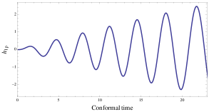
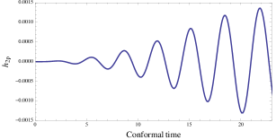
Refer to caption
Refer to caption
Figure 14: Evolution of tensor perturbations as a function of the conformal time, during early times in the radiation-dominated era for a given sub-horizon scale.

6.2.2 Early times matter-dominated era

Now, let us consider w=0𝑤0w=0 in eq. (6.13)-(6.14), and find their solutions for super-horizon and sub-horizon scales. Note that during the matter-dominated era at early times ρ~β4N2a3~𝜌subscript𝛽4superscript𝑁2proportional-tosuperscript𝑎3\tilde{\rho}\approx\beta_{4}N^{2}\propto a^{-3}, and then a2NN1/3proportional-tosuperscript𝑎2𝑁superscript𝑁13a^{2}N\propto N^{-1/3} and a2/NN7/3proportional-tosuperscript𝑎2𝑁superscript𝑁73a^{2}/N\propto N^{-7/3}. Therefore, mixing terms can be ignored in the equations of motion as N1much-greater-than𝑁1N\gg 1 at early times in this branch.

Super-horizon scales:

the evolution equations are now

h2p′′+2h2p=0,superscriptsubscript2𝑝′′2superscriptsubscript2𝑝0\displaystyle h_{2p}^{\prime\prime}+2\mathcal{H}h_{2p}^{\prime}=0, (6.21)
h1p′′h1p=0,superscriptsubscript1𝑝′′superscriptsubscript1𝑝0\displaystyle h_{1p}^{\prime\prime}-\mathcal{H}h_{1p}^{\prime}=0, (6.22)

and are solved by h2p=c1+c2/τ3subscript2𝑝subscript𝑐1subscript𝑐2superscript𝜏3h_{2p}=c_{1}+c_{2}/\tau^{3}; h1p=c3+c4τ3subscript1𝑝subscript𝑐3subscript𝑐4superscript𝜏3h_{1p}=c_{3}+c_{4}\tau^{3}, where c1subscript𝑐1c_{1}, c2subscript𝑐2c_{2}, c3subscript𝑐3c_{3} and c4subscript𝑐4c_{4} are integration constants. We find then that h1psubscript1𝑝h_{1p} grows as a power of τ𝜏\tau and h2psubscript2𝑝h_{2p} decays, in a similar way to the radiation-dominated era solutions.

sub-horizon scales:

the evolution equations simplify to

h2p′′+2h2p+x22h2p+𝒪(N1/3)(h2ph1p)=0,superscriptsubscript2𝑝′′2superscriptsubscript2𝑝superscript𝑥2superscript2subscript2𝑝𝒪superscript𝑁13subscript2𝑝subscript1𝑝0\displaystyle h_{2p}^{\prime\prime}+2\mathcal{H}h_{2p}^{\prime}+x^{2}\mathcal{H}^{2}h_{2p}+\mathcal{O}(N^{-1/3})(h_{2p}-h_{1p})=0, (6.23)
h1p′′h1p+x224h1p+𝒪(N7/3)(h1ph2p)=0,superscriptsubscript1𝑝′′superscriptsubscript1𝑝superscript𝑥2superscript24subscript1𝑝𝒪superscript𝑁73subscript1𝑝subscript2𝑝0\displaystyle h_{1p}^{\prime\prime}-\mathcal{H}h_{1p}^{\prime}+\frac{x^{2}\mathcal{H}^{2}}{4}h_{1p}+\mathcal{O}(N^{-7/3})(h_{1p}-h_{2p})=0, (6.24)

and are solved by h1p(1ikτ/2)e±ikτ/2proportional-tosubscript1𝑝minus-or-plus1𝑖𝑘𝜏2superscript𝑒plus-or-minus𝑖𝑘𝜏2h_{1p}\propto(1\mp ik\tau/2)e^{\pm ik\tau/2} and h2p(1ikτ)τ3e±ikτproportional-tosubscript2𝑝minus-or-plus1𝑖𝑘𝜏superscript𝜏3superscript𝑒plus-or-minus𝑖𝑘𝜏h_{2p}\propto\frac{(1\mp ik\tau)}{\tau^{3}}e^{\pm ik\tau}.

Fig. (15) shows numerical solutions for the evolution of tensor perturbations as a function of τ𝜏\tau (in arbitrary units), at early times in the matter-dominated era for a given sub-horizon scale. Again, in this case we set m2β1=m2β4=102superscript𝑚2subscript𝛽1superscript𝑚2subscript𝛽4superscript102m^{2}\beta_{1}=m^{2}\beta_{4}=10^{-2}, and arbitrary initial conditions of the same order for both fields. Unlike during the radiation-dominated era, in this case h1psubscript1𝑝h_{1p} grows linearly with time, but h2psubscript2𝑝h_{2p} decays.

Refer to caption
Refer to caption
Figure 15: Evolution of tensor perturbations during early times in the matter-dominated era.

We have found that h1psubscript1𝑝h_{1p} grows as a power law at early times for super-horizon and sub-horizon scales. At late times, this could mean that h1psubscript1𝑝h_{1p} could start in de-Sitter phase being some orders of magnitude higher than h2psubscript2𝑝h_{2p}. This would produce the same effect described previously for late times solutions in the expanding branch, but in this case h2psubscript2𝑝h_{2p} would grow at late times due to h1psubscript1𝑝h_{1p}.

7 Discussion

In this paper we have undertaken a comprehensive analysis of the evolution of cosmological linear perturbations in massive bigravity and have found approximate analytical solutions in a wide range of regimes. We have confirmed the main results of previous works on linear perturbations, but also extended their analysis to vector and tensor modes. In doing so we have found that massive bigravity has a number of instabilities which manifest themselves as growing solutions. In particular, we have found that most choices of parameters generate exponential instabilities in the scalar, vector or tensor modes. A subset of model space does not have exponential instabilities: when β3=β2=0subscript𝛽3subscript𝛽20\beta_{3}=\beta_{2}=0 with β1subscript𝛽1\beta_{1} and β4subscript𝛽4\beta_{4} being positive, which corresponds to a particular case of the bouncing branch. However, even for this subset of models we have found growing power-law solutions in the vector and tensor modes, contrary to GR, and a violation of the Higuchi bound, which would bring instabilities when studying the model beyond the classical linear regime. For vector and tensor fields, this growth is a consequence of a bounce in fμνsubscript𝑓𝜇𝜈f_{\mu\nu} along with effects from the interaction terms between both metrics. Analogously to scenarios with exponential instabilities, these growing modes could be a source of concern as the perturbation theory could break down at some early time. However, this latter case is not as bad because, as we will show later, we can prevent modes from growing too large by considering particular initial conditions. This resulting fine-tuning is much less restrictive than that required for the exponential solutions.

As mentioned in the introduction, such growing modes may be a hint that all is not well and that the initial values problem may not be well-posed. If indeed this is the case, it would not be surprising as extra degrees of freedom may lead to such behaviour. For example there have been efforts in trying to determine whether scalar-tensor theories have a well-posed initial value problem, while a study of Einstein-Aether theories has shown that caustics will generically arise there [41]. We believe a detailed analysis of the initial value problem in massive bigravity is essential to place it on a firm footing.

An alternative view could be to take the solutions we have found and speculate on their cosmological consequences. To do this accurately, one would have to explore the correct set of initial conditions which would arise in such a theory due to (for example) inflation. One would then have to incorporate our equations into a complete and realistic model of the universe that incorporates the various components, the correct thermal history and the Boltzmann equation for the relativistic degrees of freedom. We leave that for future work. Nevertheless, we can attempt to estimate the effect of the new solutions we have found by focusing on a few observables.

In what follows we will focus solely on tensor modes; we found a growing mode for vectors but we do not address its effect for now. Recall from the previous section that for super-horizon scales during the radiation-dominated era, h2psubscript2𝑝h_{2p} grows as τ3superscript𝜏3\tau^{3} due to the interaction terms with h1psubscript1𝑝h_{1p}. Therefore, from the end of the inflationary era until the recombination era, h2psubscript2𝑝h_{2p} might deviate substantially from its value in GR. As a result we might expect a larger effect from gravitational waves in the Cosmic Microwave Background (CMB). An estimate of how much h2psubscript2𝑝h_{2p} could grow in this stage (on super-horizon scales) gives us:

h2rech2i+(Kτeq)26[h1ih2i+τr315τih1i]+(Kτeq)29[h1ih2i+τr36τih1i](1(τeqτrec)3),subscript2recsubscript2𝑖superscript𝐾subscript𝜏eq26delimited-[]subscript1𝑖subscript2𝑖superscriptsubscript𝜏𝑟315subscript𝜏𝑖superscriptsubscript1𝑖superscript𝐾subscript𝜏eq29delimited-[]subscript1𝑖subscript2𝑖superscriptsubscript𝜏𝑟36subscript𝜏𝑖superscriptsubscript1𝑖1superscriptsubscript𝜏eqsubscript𝜏rec3h_{2{\rm rec}}\approx h_{2i}+\frac{(K\tau_{\rm eq})^{2}}{6}\left[h_{1i}-h_{2i}+\frac{\tau_{r}^{3}}{15}\tau_{i}h_{1i}^{\prime}\right]+\frac{(K\tau_{\rm eq})^{2}}{9}\left[h_{1i}-h_{2i}+\frac{\tau_{r}^{3}}{6}\tau_{i}h_{1i}^{\prime}\right]\left(1-\left(\frac{\tau_{\rm eq}}{\tau_{\rm rec}}\right)^{3}\right), (7.1)

where h2recsubscript2rech_{2{\rm rec}} is the value of the tensor perturbation h2psubscript2𝑝h_{2p} at recombination given an initial value of h2isubscript2𝑖h_{2i} at some initial time τisubscript𝜏𝑖\tau_{i}. The subindex eqeq{\rm eq} corresponds to a value at the matter-equality time, and we have defined τr=τeq/τi=aeq/aisubscript𝜏𝑟subscript𝜏eqsubscript𝜏𝑖subscript𝑎eqsubscript𝑎𝑖\tau_{r}=\tau_{\rm eq}/\tau_{i}=a_{\rm eq}/a_{i}. Here, we have also used that K2=m2a2Nβ1msuperscript𝐾2superscript𝑚2superscript𝑎2𝑁subscript𝛽1proportional-to𝑚K^{2}=m^{2}a^{2}N\beta_{1}\propto m, and Kτeq1much-less-than𝐾subscript𝜏eq1K\tau_{\rm eq}\ll 1 (which would happen for a sufficiently small m𝑚m), and calculated the first order corrections in K2superscript𝐾2K^{2}.

Note that in GR the value at the recombination era would be h2isubscript2𝑖h_{2i} for a super-horizon scale, given that h2i=0superscriptsubscript2𝑖0h_{2i}^{\prime}=0 and, therefore, the second and third terms in eq. (7.1) correspond to the modifications introduced by massive gravity to this tensor perturbation, which are proportional to m𝑚m. Even though Kτeq1much-less-than𝐾subscript𝜏𝑒𝑞1K\tau_{eq}\ll 1, the modification is not necessarily small as it depends also on the initial conditions for h1psubscript1𝑝h_{1p}.

If we choose τisubscript𝜏𝑖\tau_{i} to be the end of the inflationary era (for example where ai1028similar-tosubscript𝑎𝑖superscript1028a_{i}\sim 10^{-28}), we have that τr3τi10107similar-tosuperscriptsubscript𝜏𝑟3subscript𝜏𝑖superscript10107\tau_{r}^{3}\tau_{i}\sim 10^{107}. Therefore, we would need h1psubscript1𝑝h_{1p} to be effectively zero at the end of the inflationary era, and h1psubscript1𝑝h_{1p} would then be constant for super-horizon scales. Otherwise, h1psubscript1𝑝h_{1p}, and as a consequence h2psubscript2𝑝h_{2p}, could grow large and break the validity of perturbation theory. Assuming h1i=0superscriptsubscript1𝑖0h_{1i}^{\prime}=0 and some preferred values found in [9] when constraining scalar perturbations with observational data, the largest modification introduced by massive gravity in h2psubscript2𝑝h_{2p} at the epoch of the recombination, according to eq. (7.1), would be:

Δh2rec=h2rech2i=106(h1ih2i).Δsubscript2recsubscript2recsubscript2𝑖superscript106subscript1𝑖subscript2𝑖\Delta h_{2{\rm rec}}=h_{2{\rm rec}}-h_{2i}=10^{-6}\left(h_{1i}-h_{2i}\right). (7.2)

Further research at early times is needed in order to give exact numbers as we would need to know the initial condition for both tensor perturbations.

In a similar way, we can study the evolution for sub-horizon perturbations. For a scale that crosses the horizon during the radiation-dominated era, there will be a modification in the evolution of h2psubscript2𝑝h_{2p}, with respect to GR, coming from the interaction with h1psubscript1𝑝h_{1p}, as we can see in eq. (Sub-horizon scales:). From the horizon crossing time τcsubscript𝜏𝑐\tau_{c} until the recombination era τrecsubscript𝜏rec\tau_{\rm rec}, the modification to h2psubscript2𝑝h_{2p} is given by:

Δh2rec=(τeqτrec)2(K2k2)[c1h2c+xeq2(c2h1c+c3h1ck)],Δsubscript2recsuperscriptsubscript𝜏eqsubscript𝜏rec2superscript𝐾2superscript𝑘2delimited-[]subscript𝑐1subscript2𝑐superscriptsubscript𝑥eq2subscript𝑐2subscript1𝑐subscript𝑐3superscriptsubscript1𝑐𝑘\Delta h_{2{\rm rec}}=\left(\frac{\tau_{\rm eq}}{\tau_{\rm rec}}\right)^{2}\left(\frac{K^{2}}{k^{2}}\right)\left[c_{1}h_{2c}+x_{\rm eq}^{2}\left(c_{2}h_{1c}+c_{3}\frac{h_{1c}^{\prime}}{k}\right)\right], (7.3)

where xeq=kτeqsubscript𝑥eq𝑘subscript𝜏eqx_{\rm eq}=k\tau_{\rm eq}, and the subindex c𝑐c indicates that the quantity is evaluated at the horizon-crossing time. Here, again, we have considered only first order corrections in K2superscript𝐾2K^{2}, and the coefficients c1subscript𝑐1c_{1}, c2subscript𝑐2c_{2}, and c3subscript𝑐3c_{3} are functions of sin(xrec)subscript𝑥rec\sin(x_{\rm rec}) and cos(xrec)subscript𝑥rec\cos(x_{\rm rec}), so they all roughly have the same order of magnitude.

Note that, since in eq. (Sub-horizon scales:) h2psubscript2𝑝h_{2p} has a linear growing mode, one could have expected to have larger modifications for larger k𝑘k, as larger k𝑘k enter the horizon before and consequently spend more time growing. However, as we observe in eq. (7.3), for larger k𝑘k the modification is smaller. This happens because the coefficients c1±subscript𝑐limit-from1plus-or-minusc_{1\pm}, c2±subscript𝑐limit-from2plus-or-minusc_{2\pm} and c3±subscript𝑐limit-from3plus-or-minusc_{3\pm} in eq. (Sub-horizon scales:) are related to those of h1psubscript1𝑝h_{1p}. In particular, c3±kh1csimilar-tosubscript𝑐limit-from3plus-or-minus𝑘subscript1𝑐c_{3\pm}\sim kh_{1c}, c2±k2h1c/K2similar-tosubscript𝑐limit-from2plus-or-minussuperscript𝑘2subscript1𝑐superscript𝐾2c_{2\pm}\sim k^{2}h_{1c}/K^{2} and c1±k3h1c/K4similar-tosubscript𝑐limit-from1plus-or-minussuperscript𝑘3subscript1𝑐superscript𝐾4c_{1\pm}\sim k^{3}h_{1c}/K^{4}. Therefore, for sufficiently small m𝑚m, the dominant term will be c1±subscript𝑐limit-from1plus-or-minusc_{1\pm} and therefore the growing mode will be suppressed compared to the decaying mode, which is what actually happens for observable scales with the preferred values found in [9].

In addition, note in eq. (7.3) that, since xeq1much-greater-thansubscript𝑥eq1x_{\rm eq}\gg 1, the contribution from h1csubscript1𝑐h_{1c} to Δh2recΔsubscript2rec\Delta h_{2{\rm rec}} is much larger that the contribution from h2csubscript2𝑐h_{2c}. A numerical estimate at a scale of order 1Mpc1𝑀𝑝𝑐1Mpc gives us

Δh2rec1024h2c+105h1c+1045h1c,similar-toΔsubscript2recsuperscript1024subscript2𝑐superscript105subscript1𝑐superscript1045superscriptsubscript1𝑐\Delta h_{2{\rm rec}}\sim 10^{-24}h_{2c}+10^{-5}h_{1c}+10^{45}h_{1c}^{\prime}, (7.4)

where, again, we see that some kind of mechanism is needed to get h1c=0superscriptsubscript1𝑐0h_{1c}^{\prime}=0 at early times, in order to avoid large modifications to GR. In addition, since the value of h2recsubscript2rech_{2{\rm rec}} in GR is estimated to be h2rec(GR)1010h2csimilar-tosuperscriptsubscript2rec𝐺𝑅superscript1010subscript2𝑐h_{2{\rm rec}}^{(GR)}\sim 10^{-10}h_{2c}, the initial condition h1ch2csimilar-tosubscript1𝑐subscript2𝑐h_{1c}\sim h_{2c} will not lead to a small modification to GR. In fact, it will lead to a correction 105superscript10510^{5} times larger than the GR value, contrary to what we found on super-horizon scales according to eq. (7.2).

It is clear that, without an appropriate set of initial conditions for cosmological perturbations, we are unable to make definitive statements about the observational viability of these models. They do, however, give us an indication as to what we might expect and it seems that there might be problems with both branches of massive bigravity. The full equations presented in this paper are what is required to modify existing software packages for precise calculations of the growth of large scale structure and the evolution of the cosmic microwave background. With such machinery in hand it should be possible to explore what initial conditions are observationally viable and can be used to place stringent constraints on any theory of the early universe in massive bigravity.

Finally, it is important to remark that even if the initial value problem is not solved for the model studied in this paper, it does not mean that massive gravity should be left out as a cosmological model, as there are simple modifications to the simplest paradigm that could be explored. One simple and interesting modification can arise in eq. (3.1), as asymmetries could be introduced in fμνsubscript𝑓𝜇𝜈f_{\mu\nu}, while maintaining isotropy in gμνsubscript𝑔𝜇𝜈g_{\mu\nu}. Other changes could also be considered in the type of coupling with matter (some variations have already been studied in [42, 43, 44, 45, 46, 47, 48, 49, 50, 51, 52, 53, 54, 55, 56, 57]), or in the choices of the square root matrix g1fsuperscript𝑔1𝑓\sqrt{g^{-1}f}.

Acknowledgments

We are grateful to James Bonifacio, James Scargill, Hans Winther, Luca Amendola, Pedro Alvarez, Tessa Baker, Mariele Mota, Johannes Noller and Adam Solomon for useful discussions and comments. We are particular grateful to Marco Crisostomi for encouraging us to check the properties of the perturbations at the bounce. ML was funded by Becas Chile. PGF acknowledges support from Leverhulme, STFC, BIPAC and the Oxford Martin School.

Appendix A Scalar perturbations equations

In this section we present the relevant analysis and equations related to scalar perturbations.

A.1 Auxiliary variables

As explained in Section 3, the fields B1subscript𝐵1B_{1}, B2subscript𝐵2B_{2}, ϕ1subscriptitalic-ϕ1\phi_{1} and ϕ2subscriptitalic-ϕ2\phi_{2} appear as auxiliary variables in the equations of motion, and therefore they can be worked out in terms of the remaining fields E1subscript𝐸1E_{1}, E2subscript𝐸2E_{2} and ψ2subscript𝜓2\psi_{2}, by using their own equations of motion-namely eq. (3.21), (3.22), (3.25) and (3.26). The explicit expressions for the four auxiliary variables are:

B2subscript𝐵2\displaystyle B_{2} =1Da[k2(32Za2m2X+k2N(1+X))E2+32k2N2a2E1m2Z\displaystyle=\frac{1}{D_{a}}\left[k^{2}\left(\frac{3}{2}Za^{2}m^{2}X+k^{2}N(1+X)\right)\mathcal{H}E_{2}^{\prime}+\frac{3}{2}\mathcal{H}k^{2}N^{2}a^{2}E_{1}^{\prime}m^{2}Z\right.
+34ρm2XZ(1+w)(3ψ2+k2E2)a4+12(m2Z(1+X)(k2E2k2E1+3ψ2)N2\displaystyle+\frac{3}{4}\rho_{*}m^{2}XZ(1+w)(3\psi_{2}+k^{2}E_{2})a^{4}+\frac{1}{2}\left(m^{2}Z(1+X)(k^{2}E_{2}-k^{2}E_{1}+3\psi_{2})N^{2}\right.
+ρ(1+X)(1+w)(3ψ2+k2E2)N+3m2XZψ2)k2a2+ψ2k4N(1+X)],\displaystyle\left.\left.+\rho_{*}(1+X)(1+w)\left(3\psi_{2}+k^{2}E_{2}\right)N+3m^{2}XZ\psi_{2}\right)k^{2}a^{2}+\psi_{2}k^{4}N(1+X)\right], (A.1)
B1subscript𝐵1\displaystyle B_{1} =14XDa[4Nk2E1(32a2(ρX(1+w)+Nm2Z+ρ(1+w))+k2(1+X))\displaystyle=\frac{1}{4XD_{a}}\left[4Nk^{2}\mathcal{H}E_{1}^{\prime}\left(\frac{3}{2}a^{2}\left(\rho_{*}X(1+w)+Nm^{2}Z+\rho_{*}(1+w)\right)+k^{2}(1+X)\right)\right.
2Za2Xm2(3k2E2+32((k2E2k2E1+3ψ2)Xk2E1)(1+w)ρa2\displaystyle-2Za^{2}Xm^{2}\left(-3k^{2}\mathcal{H}E_{2}^{\prime}+\frac{3}{2}\left((k^{2}E_{2}-k^{2}E_{1}+3\psi_{2})X-k^{2}E_{1}\right)(1+w)\rho_{*}a^{2}\right.
+k2((k2E2k2E1+3ψ2)X+k2(E2E1)))],\displaystyle\left.\left.+k^{2}\left((k^{2}E_{2}-k^{2}E_{1}+3\psi_{2})X+k^{2}(E_{2}-E_{1})\right)\right)\right], (A.2)
ϕ2subscriptitalic-ϕ2\displaystyle\phi_{2} =18Da[8ψ2(94ρm2XZ(1+w)a4+32k2a2(ρ(1+X)(1+w)N+m2Z(X+N2))\displaystyle=\frac{-1}{8\mathcal{H}D_{a}}\left[8\mathcal{H}\psi_{2}^{\prime}\left(\frac{9}{4}\rho_{*}m^{2}XZ(1+w)a^{4}+\frac{3}{2}k^{2}a^{2}\left(\rho_{*}(1+X)(1+w)N+m^{2}Z(X+N^{2})\right)\right.\right.
+k4N(1+X))+2a2(2k2(32ρm2XZ(1+w)a2+N(ρ(1+X)(1+w))k2\displaystyle\left.+k^{4}N(1+X)\frac{}{}\right)+2a^{2}\left(2k^{2}\mathcal{H}\left(\frac{3}{2}\rho_{*}m^{2}XZ(1+w)a^{2}+N(\rho_{*}(1+X)(1+w))k^{2}\right.\right.
+Nm2Z)E22m2N2Zk4E1+32ZX(1+w)ρm2a4(ρ(1+w)(3ψ2+k2E2)\displaystyle\left.+Nm^{2}Z\frac{}{}\right)E_{2}^{\prime}-2m^{2}N^{2}Z\mathcal{H}k^{4}E_{1}^{\prime}+\frac{3}{2}ZX(1+w)\rho_{*}m^{2}a^{4}\left(\rho_{*}(1+w)(3\psi_{2}+k^{2}E_{2})\right.
+m2Z(k2E2k2E1+3ψ2)N)+k2a2(N(1+w)2(1+X)(3ψ2+k2E2)ρ2+\displaystyle\left.+m^{2}Z(k^{2}E_{2}-k^{2}E_{1}+3\psi_{2})N\right)+k^{2}a^{2}\left(N(1+w)^{2}(1+X)(3\psi_{2}+k^{2}E_{2})\rho_{*}^{2}+\right.
Z(1+w)m2ρ(3Xψ2+N2(X(k2E2k2E1+3ψ2)+2k2E2k2E1+6ψ2))𝑍1𝑤superscript𝑚2subscript𝜌3𝑋subscript𝜓2superscript𝑁2𝑋superscript𝑘2subscript𝐸2superscript𝑘2subscript𝐸13subscript𝜓22superscript𝑘2subscript𝐸2superscript𝑘2subscript𝐸16subscript𝜓2\displaystyle Z(1+w)m^{2}\rho_{*}\left(3X\psi_{2}+N^{2}(X(k^{2}E_{2}-k^{2}E_{1}+3\psi_{2})+2k^{2}E_{2}-k^{2}E_{1}+6\psi_{2})\right)
+Nm4Z2(X+N2)(k2E2k2E1+3ψ2))+2N(Nm2Z+ρ(1+X)(1+w))ψ2k4)],\displaystyle\left.\left.\left.+Nm^{4}Z^{2}(X+N^{2})(k^{2}E_{2}-k^{2}E_{1}+3\psi_{2})\right)+2N\left(Nm^{2}Z+\rho_{*}(1+X)(1+w)\right)\psi_{2}k^{4}\frac{}{}\right)\right], (A.3)
ϕ1subscriptitalic-ϕ1\displaystyle\phi_{1} =Za2m24NDa[Nk2E1(3ρ(1+w)a2+2k2)+32ρm2XZ(1+w)(k2E2k2E1+3ψ2)a4\displaystyle=\frac{Za^{2}m^{2}}{4\mathcal{H}ND_{a}}\left[-Nk^{2}\mathcal{H}E_{1}^{\prime}(3\rho_{*}(1+w)a^{2}+2k^{2})+\frac{3}{2}\rho_{*}m^{2}XZ(1+w)(k^{2}E_{2}-k^{2}E_{1}+3\psi_{2})a^{4}\right.
+k2a2(m2Z(k2E2k2E1+3ψ2)N2+ρ(1+w)(3ψ2+k2E2)N\displaystyle+k^{2}a^{2}\left(m^{2}Z(k^{2}E_{2}-k^{2}E_{1}+3\psi_{2})N^{2}+\rho_{*}(1+w)(3\psi_{2}+k^{2}E_{2})N\right.
+m2XZ(k2E2k2E1+3ψ2))+2k4E2N+2ψ2k4N],\displaystyle\left.\left.+m^{2}XZ(k^{2}E_{2}-k^{2}E_{1}+3\psi_{2})\right)+2\mathcal{H}k^{4}E_{2}^{\prime}N+2\psi_{2}k^{4}N\right], (A.4)

where Dasubscript𝐷𝑎D_{a} is given by:

Dasubscript𝐷𝑎\displaystyle D_{a} =[32k2a2(m2N2Z+ρ(1+X)(1+w)N+m2XZ)+k4N(1+X)\displaystyle=\mathcal{H}\left[\frac{3}{2}k^{2}a^{2}\left(m^{2}N^{2}Z+\rho_{*}(1+X)(1+w)N+m^{2}XZ\right)+k^{4}N(1+X)\right.
+94ρm2XZ(1+w)a4]\displaystyle\left.+\frac{9}{4}\rho_{*}m^{2}XZ(1+w)a^{4}\frac{}{}\right] (A.5)

At a first glance, one might expect that the original system of equations (3.21)-(3.27), with seven scalar fields, has three dynamical degrees of freedom, as the equations of motion for E1subscript𝐸1E_{1}, E2subscript𝐸2E_{2} and ψ2subscript𝜓2\psi_{2} are independent and contain second derivatives. However, when eliminating the four auxiliary variables, and replacing them in the three remaining equations, we get that, in eq. (3.23) all first and second derivatives of ψ2subscript𝜓2\psi_{2} cancel out, so that ψ2subscript𝜓2\psi_{2} becomes an explicit auxiliary variable. Therefore, it can be written in terms of E1subscript𝐸1E_{1} and E2subscript𝐸2E_{2}. Next, we show the expression for ψ2subscript𝜓2\psi_{2} when worked out from eq. (3.23):

ψ2subscript𝜓2\displaystyle\psi_{2} =k22Dp[2k2N2E1(32m2Za2(X1)N2+(32X+32+k2)N+32a2m2Z(X1))\displaystyle=\frac{k^{2}}{2D_{p}}\left[-2\mathcal{H}k^{2}N^{2}E_{1}^{\prime}\left(\frac{3}{2}m^{2}Za^{2}(X-1)N^{2}+(-3\mathcal{H}^{2}X+3\mathcal{H}^{2}+k^{2})N+\frac{3}{2}a^{2}m^{2}Z(X-1)\right)\right.
+2k4N3E2+32k2X2Z2a4m4(E1E2X)N5+(E1E2X)m2a2(94m4Xa4(X1)Z2\displaystyle+2k^{4}\mathcal{H}N^{3}E_{2}^{\prime}+\frac{3}{2}k^{2}X^{2}Z^{2}a^{4}m^{4}(E_{1}-E_{2}X)N^{5}+(E_{1}-E_{2}X)m^{2}a^{2}\left(\frac{9}{4}m^{4}Xa^{4}(X-1)Z^{2}\right.
+k2(k2X6X22+32))ZN4+(32m4a4(2X3E2(k232)\displaystyle\left.+k^{2}(k^{2}X-6X^{2}\mathcal{H}^{2}+3\mathcal{H}^{2})\frac{}{}\right)ZN^{4}+\left(\frac{3}{2}m^{4}a^{4}\left(-2X^{3}E_{2}(k^{2}-3\mathcal{H}^{2})\right.\right.
+(k2E162(E2+E1))X2+2E1(32+k2)Xk2E1)Z222k2(3X3E22\displaystyle+\left.\left(k^{2}E_{1}-6\mathcal{H}^{2}(E_{2}+E_{1})\right)X^{2}+2E_{1}(3\mathcal{H}^{2}+k^{2})X-k^{2}E_{1}\right)Z^{2}-2\mathcal{H}^{2}k^{2}\left(3X^{3}E_{2}\mathcal{H}^{2}\right.
(k2E2+32E1)X2+(k2E13E22)X+32E1+k2(E2+E1)))N3\displaystyle\left.\left.-(k^{2}E_{2}+3\mathcal{H}^{2}E_{1})X^{2}+(k^{2}E_{1}-3E_{2}\mathcal{H}^{2})X+3\mathcal{H}^{2}E_{1}+k^{2}(-E_{2}+E_{1})\right)\frac{}{}\right)N^{3}
+(92m4Xa4(X1)(E1E2X)Z2+(9E24+6k22E2)X3\displaystyle+\left(\frac{9}{2}m^{4}Xa^{4}(X-1)(E_{1}-E_{2}X)Z^{2}+(-9E_{2}\mathcal{H}^{4}+6k^{2}\mathcal{H}^{2}E_{2})X^{3}\right.
(k232)(32(E1+E2)+k2E2)X2+(94E16k22(E1+12E2)+k4E2)Xsuperscript𝑘23superscript23superscript2subscript𝐸1subscript𝐸2superscript𝑘2subscript𝐸2superscript𝑋29superscript4subscript𝐸16superscript𝑘2superscript2subscript𝐸112subscript𝐸2superscript𝑘4subscript𝐸2𝑋\displaystyle-(k^{2}-3\mathcal{H}^{2})\left(3\mathcal{H}^{2}(E_{1}+E_{2})+k^{2}E_{2}\right)X^{2}+\left(-9\mathcal{H}^{4}E_{1}-6k^{2}\mathcal{H}^{2}\left(E_{1}+\frac{1}{2}E_{2}\right)+k^{4}E_{2}\right)X
+(62E1+k2(E2+E1))k2)m2a2ZN2+3m4a4(12E2(k262)X312k2E1\displaystyle\left.+\left(6\mathcal{H}^{2}E_{1}+k^{2}(-E_{2}+E_{1})\right)k^{2}\frac{}{}\right)m^{2}a^{2}ZN^{2}+3m^{4}a^{4}\left(-\frac{1}{2}E_{2}(k^{2}-6\mathcal{H}^{2})X^{3}-\frac{1}{2}k^{2}E_{1}\right.
32(E1+E2)X2+E1(32+k2)X)Z2N+94m6XZ3a6(X1)(E1E2X)],\displaystyle\left.\left.-3\mathcal{H}^{2}(E_{1}+E_{2})X^{2}+E_{1}\left(3\mathcal{H}^{2}+k^{2}\right)X\right)Z^{2}N+\frac{9}{4}m^{6}XZ^{3}a^{6}(X-1)(E_{1}-E_{2}X)\frac{}{}\right], (A.6)

where Dpsubscript𝐷𝑝D_{p} is given by

Dpsubscript𝐷𝑝\displaystyle D_{p} =X[3m2a2(98m4Xa4(X1)Z2+(k2X+3223X22)k2)ZN4\displaystyle=X\left[3m^{2}a^{2}\left(\frac{9}{8}m^{4}Xa^{4}(X-1)Z^{2}+\left(k^{2}X+\frac{3}{2}\mathcal{H}^{2}-3X^{2}\mathcal{H}^{2}\right)k^{2}\right)ZN^{4}\right.
+94X2m4Z2a4k2N5+(92m4a4((k232)X2+(12k2+32)X12k2)Z2\displaystyle+\frac{9}{4}X^{2}m^{4}Z^{2}a^{4}k^{2}N^{5}+\left(\frac{9}{2}m^{4}a^{4}\left((k^{2}-3\mathcal{H}^{2})X^{2}+\left(\frac{1}{2}k^{2}+3\mathcal{H}^{2}\right)X-\frac{1}{2}k^{2}\right)Z^{2}\right.
6k4X29k24+9X2k24+k6)N3+3m2a2ZN2(94m4Xa4(X1)Z2\displaystyle\left.-6k^{4}X\mathcal{H}^{2}-9k^{2}\mathcal{H}^{4}+9X^{2}k^{2}\mathcal{H}^{4}+k^{6}\frac{}{}\right)N^{3}+3m^{2}a^{2}ZN^{2}\left(\frac{9}{4}m^{4}Xa^{4}(X-1)Z^{2}\right.
+(92432k2)X2+(k4924322k2)X+32k2)\displaystyle\left.+\left(\frac{9}{2}\mathcal{H}^{4}-3\mathcal{H}^{2}k^{2}\right)X^{2}+\left(k^{4}-\frac{9}{2}\mathcal{H}^{4}-\frac{3}{2}\mathcal{H}^{2}k^{2}\right)X+3\mathcal{H}^{2}k^{2}\right)
+94m4a4((k262)X2+(k2+62)Xk2)Z2N+278m6XZ3a6(X1)].\displaystyle\left.+\frac{9}{4}m^{4}a^{4}\left(\left(k^{2}-6\mathcal{H}^{2}\right)X^{2}+\left(k^{2}+6\mathcal{H}^{2}\right)X-k^{2}\right)Z^{2}N+\frac{27}{8}m^{6}XZ^{3}a^{6}(X-1)\right]. (A.7)

Therefore, as expected, only two degrees of freedoms are remain: E1subscript𝐸1E_{1} and E2subscript𝐸2E_{2}.

A.2 Complete equations of motion

In this subsection we present the full equations of motion for the two propagating, physical scalar degrees of freedom: E1subscript𝐸1E_{1} and E2subscript𝐸2E_{2}. The equation for E2subscript𝐸2E_{2} takes the following form:

E2′′274D2(w+13)k2N2a4ρm2Z(1+w)E13D2[32(1+w)2a4(32a2Xm2Z\displaystyle E_{2}^{{}^{\prime\prime}}-\frac{27}{4D_{2}}\left(w+\frac{1}{3}\right)k^{2}N^{2}a^{4}\rho_{*}m^{2}\mathcal{H}Z(1+w)E_{1}^{\prime}-\frac{3\mathcal{H}}{D_{2}}\left[-\frac{3}{2}(1+w)^{2}a^{4}\left(\frac{3}{2}a^{2}Xm^{2}Z\right.\right.
+k2N(1+X))ρ2+12(1+w)(32m2a2Z((3w1)X2N2)+k2N(3(w1)X+3w\displaystyle\left.\left.+k^{2}N(1+X)\frac{}{}\right)\rho_{*}^{2}+\frac{1}{2}(1+w)\left(\frac{3}{2}m^{2}a^{2}Z\left(\left(3w-1\right)X-2N^{2}\right)+k^{2}N\left(3(w-1)X+3w\right.\right.\right.
+1))a2k2ρ+(X1)k6N(w13)]E2+k2D2[k6Nw(X1)\displaystyle\left.\left.\left.+1\right)\frac{}{}\right)a^{2}k^{2}\rho_{*}+(X-1)k^{6}N\left(w-\frac{1}{3}\right)\right]E_{2}^{\prime}+\frac{k^{2}}{D_{2}}\left[k^{6}Nw(X-1)\right.
34(1+w)2a4(32a2Xm2Z+k2N(1+X))ρ2+12a2(1+w)k2ρ{32Zm2a2(3Xw\displaystyle-\frac{3}{4}(1+w)^{2}a^{4}\left(\frac{3}{2}a^{2}Xm^{2}Z+k^{2}N(1+X)\right)\rho_{*}^{2}+\frac{1}{2}a^{2}(1+w)k^{2}\rho_{*}\left\{\frac{3}{2}Zm^{2}a^{2}\left(3Xw\right.\right.
+N2((3w+1)X1))+Nk2((3w1)X+3w+1)}]E2\displaystyle\left.\left.\left.+N^{2}\left(\left(3w+1\right)X-1\right)\right)+Nk^{2}\left(\left(3w-1\right)X+3w+1\right)\right\}\right]E_{2}
+m2D2a2N[94k2Z~ρm2a4Z(1+w)N2+k2{3(1+w)(Z~(1+3w)Z4)k2Xρa2\displaystyle+\frac{m^{2}}{D_{2}}a^{2}N\left[\frac{9}{4}k^{2}\tilde{Z}\rho_{*}m^{2}a^{4}Z(1+w)N^{2}+k^{2}\left\{3(1+w)\left(\tilde{Z}-(1+3w)\frac{Z}{4}\right)k^{2}X\rho_{*}a^{2}\right.\right.
+94Z~ρ2(1+w)2(1+X)a4+(Z~32(w+13)Z)k4(X1)}N\displaystyle\left.+\frac{9}{4}\tilde{Z}\rho_{*}^{2}(1+w)^{2}(1+X)a^{4}+\left(\tilde{Z}-\frac{3}{2}\left(w+\frac{1}{3}\right)Z\right)k^{4}(X-1)\right\}N
+94(1+w)Z~ZXρm2a4(32ρ(1+w)a2+k2)](E2E1)=0,\displaystyle\left.+\frac{9}{4}(1+w)\tilde{Z}ZX\rho_{*}m^{2}a^{4}\left(\frac{3}{2}\rho_{*}(1+w)a^{2}+k^{2}\right)\right](E_{2}-E_{1})=0, (A.8)

and the equation for E1subscript𝐸1E_{1} takes the following form:

E1′′+2D1[94a4{34a2m2(4X2+(3w1)X(1+3w))Z2+12(3X2+(3w+1)X\displaystyle E_{1}^{{}^{\prime\prime}}+\frac{2\mathcal{H}}{D_{1}}\left[\frac{9}{4}a^{4}\left\{\frac{3}{4}a^{2}m^{2}\left(4X^{2}+\left(3w-1\right)X-\left(1+3w\right)\right)Z^{2}+\frac{1}{2}\left(3X^{2}+\left(3w+1\right)X\right.\right.\right.
3w)k2NZ+NZ~k2(1+X)}(1+w)3Nρ3+3a2{916a4m4(1+X)(X1)2(N2+1)Z3\displaystyle\left.\left.-3w\right)k^{2}NZ+N\tilde{Z}k^{2}(1+X)\right\}(1+w)^{3}N\rho_{*}^{3}+3a^{2}\left\{-\frac{9}{16}a^{4}m^{4}(1+X)(X-1)^{2}(N^{2}+1)Z^{3}\right.
98a2m2Z2(13k2N(N2X(X2X1)+X3+2+3w(1X+N2)5X2)\displaystyle-\frac{9}{8}a^{2}m^{2}Z^{2}\left(\frac{1}{3}k^{2}N\left(N^{2}X(X^{2}-X-1)+X^{3}+2+3w(1-X+N^{2})-5X^{2}\right)\right.
m2Z~(X1)2(N2+1)a2)+34k2(m2Z~(X1)2(N2+1)a2\displaystyle\left.-m^{2}\tilde{Z}(X-1)^{2}(N^{2}+1)a^{2}\frac{}{}\right)+\frac{3}{4}k^{2}\left(m^{2}\tilde{Z}(X-1)^{2}(N^{2}+1)a^{2}\right.
+(2X2+(w13)X(w+13))k2N)NZ+Z~k4N2X}(1+w)2ρ2\displaystyle\left.\left.+\left(2X^{2}+\left(w-\frac{1}{3}\right)X-\left(w+\frac{1}{3}\right)\right)k^{2}N\right)NZ+\tilde{Z}k^{4}N^{2}X\right\}(1+w)^{2}\rho_{*}^{2}
+k2(X1){98a4m4(X1)(1+X)(N2+1)Z332a2(N2+1)(X1)m2(Nk2(1+X)\displaystyle+k^{2}(X-1)\left\{-\frac{9}{8}a^{4}m^{4}(X-1)(1+X)(N^{2}+1)Z^{3}-\frac{3}{2}a^{2}(N^{2}+1)(X-1)m^{2}\left(\frac{}{}Nk^{2}(1+X)\right.\right.
32m2a2Z~)Z2+12(6m2Z~(N2+1)(X1)a2+(1+3X)k2N)k2NZ+k4Z~N2}(1+w)ρ\displaystyle\left.\left.-\frac{3}{2}m^{2}a^{2}\tilde{Z}\right)Z^{2}+\frac{1}{2}\left(6m^{2}\tilde{Z}(N^{2}+1)(X-1)a^{2}+\left(1+3X\right)k^{2}N\right)k^{2}NZ+k^{4}\tilde{Z}N^{2}\right\}(1+w)\rho_{*}
+(N2+1)k6(X1)2Zm2N(Z~12(X+1)Z)]E1\displaystyle\left.+(N^{2}+1)k^{6}(X-1)^{2}Zm^{2}N\left(\tilde{Z}-\frac{1}{2}(X+1)Z\right)\right]E_{1}^{\prime}
2k2D1[98a4ρm4(1+X)(X1)2(N2+1)(1+w)Z312m2Z2{k4N(X1)2(1\displaystyle-2\frac{\mathcal{H}k^{2}}{D_{1}}\left[-\frac{9}{8}a^{4}\rho_{*}m^{4}(1+X)(X-1)^{2}(N^{2}+1)(1+w)Z^{3}-\frac{1}{2}m^{2}Z^{2}\left\{\frac{}{}k^{4}N(X-1)^{2}(1\right.\right.
+X)(N2+1)272(23X2+(w13)X12w16)a4(1+w)2Nρ2+32(Nk2(1+X)\displaystyle+X)(N^{2}+1)-\frac{27}{2}\left(\frac{2}{3}X^{2}+\left(w-\frac{1}{3}\right)X-\frac{1}{2}w-\frac{1}{6}\right)a^{4}(1+w)^{2}N\rho_{*}^{2}+\frac{3}{2}\left(Nk^{2}(1+X)\right.
+continues in next pagecontinues in next page\displaystyle+\mbox{continues in next page}
3m2a2Z~)a2(1+w)(N2+1)(X1)2ρ}+k2NZ(92a2(1+w)2(Xw+12X216)Nρ2\displaystyle\left.\left.-3m^{2}a^{2}\tilde{Z}\right)a^{2}(1+w)(N^{2}+1)(X-1)^{2}\rho_{*}\right\}+k^{2}NZ\left(\frac{9}{2}a^{2}(1+w)^{2}\left(Xw+\frac{1}{2}X^{2}-\frac{1}{6}\right)N\rho_{*}^{2}\right.
+32(1+w)(X1)(m2a2Z~(X1)N2+k2(X+w)N+m2a2Z~(X1))ρ321𝑤𝑋1superscript𝑚2superscript𝑎2~𝑍𝑋1superscript𝑁2superscript𝑘2𝑋𝑤𝑁superscript𝑚2superscript𝑎2~𝑍𝑋1subscript𝜌\displaystyle+\frac{3}{2}(1+w)(X-1)\left(m^{2}a^{2}\tilde{Z}(X-1)N^{2}+k^{2}(X+w)N+m^{2}a^{2}\tilde{Z}(X-1)\right)\rho_{*}
+k2Z~m2(X1)2(N2+1))+(32a2(1+X)(1+w)ρ+k2(X1))ρZ~(1+w)k2N2]E2\displaystyle\left.\left.+k^{2}\tilde{Z}m^{2}(X-1)^{2}(N^{2}+1)\frac{}{}\right)+\left(\frac{3}{2}a^{2}(1+X)(1+w)\rho_{*}+k^{2}(X-1)\right)\rho_{*}\tilde{Z}(1+w)k^{2}N^{2}\right]E_{2}^{\prime}
+ρk2(1+w)D1[34m4Z2((1+X)Z2Z~)a4k2(X1)2N412{3ρ((12X3+2X2\displaystyle+\frac{\rho_{*}k^{2}(1+w)}{D_{1}}\left[-\frac{3}{4}m^{4}Z^{2}\left((1+X)Z-2\tilde{Z}\right)a^{4}k^{2}(X-1)^{2}N^{4}-\frac{1}{2}\left\{-3\rho_{*}\left(\left(-\frac{1}{2}X^{3}+2X^{2}\right.\right.\right.\right.
+(3w12)X32w1)Z+Z~(X1)2)(1+w)a2+k2(X1)2((1+X)Z\displaystyle\left.+\left(3w-\frac{1}{2}\right)X-\frac{3}{2}w-1\right)Z\left.+\tilde{Z}(X-1)^{2}\right)(1+w)a^{2}+k^{2}(X-1)^{2}((1+X)Z
2Z~)}m2Za2k2N3+{(32m4(1+X)(X1)2Z3+3m4Z~(X1)2Z2+34(X23w\displaystyle\left.-2\tilde{Z})\frac{}{}\right\}m^{2}Za^{2}k^{2}N^{3}+\left\{\left(-\frac{3}{2}m^{4}(1+X)(X-1)^{2}Z^{3}+3m^{4}\tilde{Z}(X-1)^{2}Z^{2}+\frac{3}{4}\left(X^{2}-3w\right.\right.\right.
+(3w2)X1)ρ2(1+w)2Z32ρ2XZ~(1+w)2(1+X))a4+12ρa2k2(1+w)((1\displaystyle\left.\left.+\left(3w-2\right)X-1\right)\rho_{*}^{2}(1+w)^{2}Z-\frac{3}{2}\rho_{*}^{2}X\tilde{Z}(1+w)^{2}(1+X)\right)a^{4}+\frac{1}{2}\rho_{*}a^{2}k^{2}(1+w)\left(\frac{}{}\left(-1\right.\right.
+(2+3w)X2+(3w1)X)Z4Z~(12+X)(X1))+13((1+(1+3w)X)Z\displaystyle\left.\left.+\left(2+3w\right)X^{2}+\left(3w-1\right)X\right)Z-4\tilde{Z}\left(\frac{1}{2}+X\right)(X-1)\right)+\frac{1}{3}\left(\left(-1+\left(1+3w\right)X\right)Z\right.
2Z~(X1))k4(X1)}k2N212m2Za2{94ZX3ρ2(1+w)2a43k2(1+w)(Z~(X1)2\displaystyle\left.\left.-2\tilde{Z}(X-1)\right)k^{4}(X-1)\right\}k^{2}N^{2}-\frac{1}{2}m^{2}Za^{2}\left\{\frac{9}{4}ZX^{3}\rho_{*}^{2}(1+w)^{2}a^{4}-3k^{2}(1+w)\left(\tilde{Z}(X-1)^{2}\right.\right.
+Z(X3+52X2+(12+3w)X32w1))ρa2+((1+X)Z2Z~)k4(X1)2}N\displaystyle\left.\left.+Z\left(-X^{3}+\frac{5}{2}X^{2}+\left(-\frac{1}{2}+3w\right)X-\frac{3}{2}w-1\right)\right)\rho_{*}a^{2}+((1+X)Z-2\tilde{Z})k^{4}(X-1)^{2}\right\}N
34m4Z2((1+X)Z2Z~)a4k2(X1)2]E1+1D1[a2(X1)2m4Z2k6N4(Z~\displaystyle\left.-\frac{3}{4}m^{4}Z^{2}\left((1+X)Z-2\tilde{Z}\right)a^{4}k^{2}(X-1)^{2}\right]E_{1}+\frac{1}{D_{1}}\left[-a^{2}(X-1)^{2}m^{4}Z^{2}k^{6}N^{4}\left(\tilde{Z}\right.\right.
(X+1)Z2)23m2Zk4{12(X1)k2Z(32ρ(1+3XX2+3w)(1+w)a2+(X2\displaystyle\left.\left.-(X+1)\frac{Z}{2}\right)-\frac{2}{3}m^{2}Zk^{4}\left\{-\frac{1}{2}(X-1)k^{2}Z\left(-\frac{3}{2}\rho_{*}\left(1+3X-X^{2}+3w\right)(1+w)a^{2}+(X^{2}\right.\right.\right.
1)k2)+(94ρ2(1+w)2(1+X)a4+32ρk2X(X1)(1+w)a2+k4(X1)2)Z~}N3\displaystyle\left.\left.-1)k^{2}\frac{}{}\right)+\left(\frac{9}{4}\rho_{*}^{2}(1+w)^{2}(1+X)a^{4}+\frac{3}{2}\rho_{*}k^{2}X(X-1)(1+w)a^{2}+k^{4}(X-1)^{2}\right)\tilde{Z}\right\}N^{3}
23k2{32k4m4a2(1+X)(X1)2Z3+3a2m4(98ρ2X(1+w)2a4+k4(X1)2)Z~Z2\displaystyle-\frac{2}{3}k^{2}\left\{-\frac{3}{2}k^{4}m^{4}a^{2}(1+X)(X-1)^{2}Z^{3}+3a^{2}m^{4}\left(\frac{9}{8}\rho_{*}^{2}X(1+w)^{2}a^{4}+k^{4}(X-1)^{2}\right)\tilde{Z}Z^{2}\right.
32ρ(32ρ(X2w+23X+w)(1+w)a2+(X1)k2(Xw13))k4(1+w)Z32subscript𝜌32subscript𝜌superscript𝑋2𝑤23𝑋𝑤1𝑤superscript𝑎2𝑋1superscript𝑘2𝑋𝑤13superscript𝑘41𝑤𝑍\displaystyle-\frac{3}{2}\rho_{*}\left(\frac{3}{2}\rho_{*}\left(X^{2}w+\frac{2}{3}X+w\right)(1+w)a^{2}+(X-1)k^{2}\left(Xw-\frac{1}{3}\right)\right)k^{4}(1+w)Z
+ρ(32a2(1+X)(1+w)ρ+k2(X1))Z~k2(32a2(1+X)(1+w)ρ+k2X)(1+w)}N2\displaystyle\left.+\rho_{*}\left(\frac{3}{2}a^{2}(1+X)(1+w)\rho_{*}+k^{2}(X-1)\right)\tilde{Z}k^{2}\left(\frac{3}{2}a^{2}(1+X)(1+w)\rho_{*}+k^{2}X\right)(1+w)\right\}N^{2}
23m2Zk2{12(94ρ2X(X21+(1+3w)X)(1+w)2a4+92ρ(X1)(23X223w\displaystyle-\frac{2}{3}m^{2}Zk^{2}\left\{-\frac{1}{2}\left(\frac{9}{4}\rho_{*}^{2}X\left(X^{2}-1+\left(1+3w\right)X\right)(1+w)^{2}a^{4}+\frac{9}{2}\rho_{*}(X-1)\left(\frac{2}{3}X^{2}-\frac{2}{3}-w\right.\right.\right.
+(w23)X)k2(1+w)a2+k4(1+X)(X1)2)k2Z+Z~(32ρ(1+w)a2+k2)\displaystyle\left.+\left(w-\frac{2}{3}\right)X\right)k^{2}(1+w)a^{2}\left.+k^{4}(1+X)(X-1)^{2}\frac{}{}\right)k^{2}Z+\tilde{Z}\left(\frac{3}{2}\rho_{*}(1+w)a^{2}+k^{2}\right)
(92ρ2X(1+w)2(1+X)a4+3ρk2X(X1)(1+w)a2+k4(X1)2)}N\displaystyle\left.\cdot\left(\frac{9}{2}\rho_{*}^{2}X(1+w)^{2}(1+X)a^{4}+3\rho_{*}k^{2}X(X-1)(1+w)a^{2}+k^{4}(X-1)^{2}\frac{}{}\right)\right\}N
a2(Z~(278X2ρ3(1+w)3a6+94k2ρ2X2(1+w)2a4+k6(X1)2)\displaystyle-a^{2}\left(\tilde{Z}\left(\frac{27}{8}X^{2}\rho_{*}^{3}(1+w)^{3}a^{6}+\frac{9}{4}k^{2}\rho_{*}^{2}X^{2}(1+w)^{2}a^{4}+k^{6}(X-1)^{2}\right)\right.
k62(1+X)(X1)2Z)m4Z2](E2E1)=0,\displaystyle\left.\left.-\frac{k^{6}}{2}(1+X)(X-1)^{2}Z\right)m^{4}Z^{2}\right](E_{2}-E_{1})=0, (A.9)

where D1subscript𝐷1D_{1} and D2subscript𝐷2D_{2} are given by:

D1=subscript𝐷1absent\displaystyle D_{1}= Zρ(1+w)N[94ρm2(N2k2+(32ρ(1+w)a2+k2)X)a4(1+w)Z\displaystyle Z\rho_{*}(1+w)N\left[\frac{9}{4}\rho_{*}m^{2}\left(N^{2}k^{2}+\left(\frac{3}{2}\rho_{*}(1+w)a^{2}+k^{2}\right)X\right)a^{4}(1+w)Z\right.
+(32ρ(1+X)(1+w)a2+k2(X1))(32ρ(1+w)a2+k2)Nk2]\displaystyle\left.+\left(\frac{3}{2}\rho_{*}(1+X)(1+w)a^{2}+k^{2}(X-1)\right)\left(\frac{3}{2}\rho_{*}(1+w)a^{2}+k^{2}\right)Nk^{2}\right] (A.10)
D2=subscript𝐷2absent\displaystyle D_{2}= 278m2ZXρ2(1+w)2a6+94k2ρ(m2(X+N2)Z+ρ(1+X)(1+w)N)(1+w)a4278superscript𝑚2𝑍𝑋superscriptsubscript𝜌2superscript1𝑤2superscript𝑎694superscript𝑘2subscript𝜌superscript𝑚2𝑋superscript𝑁2𝑍subscript𝜌1𝑋1𝑤𝑁1𝑤superscript𝑎4\displaystyle\frac{27}{8}m^{2}ZX\rho_{*}^{2}(1+w)^{2}a^{6}+\frac{9}{4}k^{2}\rho_{*}\left(m^{2}(X+N^{2})Z+\rho_{*}(1+X)(1+w)N\right)(1+w)a^{4}
+3k4ρNX(1+w)a2+k6N(X1).3superscript𝑘4subscript𝜌𝑁𝑋1𝑤superscript𝑎2superscript𝑘6𝑁𝑋1\displaystyle+3k^{4}\rho_{*}NX(1+w)a^{2}+k^{6}N(X-1). (A.11)

A.3 Exponential instabilities

As mentioned previously, in the expanding branch scalar perturbations have an exponential instability at early times for sub-horizon scales; the instability is independent of the particular values of the parameters β𝛽\betas. However, during the bouncing branch, different solutions can be found for different parameters. For this reason, we distinguish the following cases: (a) β30subscript𝛽30\beta_{3}\not=0; (b) β3=0subscript𝛽30\beta_{3}=0 and (β43β2)0subscript𝛽43subscript𝛽20(\beta_{4}-3\beta_{2})\not=0; (c)β3=0subscript𝛽30\beta_{3}=0 and (β43β2)=0subscript𝛽43subscript𝛽20(\beta_{4}-3\beta_{2})=0; (d) β3=β2=0subscript𝛽3subscript𝛽20\beta_{3}=\beta_{2}=0.

In what follows we will see that in cases (a), (b) and (c), E1subscript𝐸1E_{1} develop an exponential instability at early times. For simplicity, let us study the equations of motion during the radiation-dominated era for sub-horizon scales. Generically, the equations of motion can be written as

Ea′′+fab(x,N)Eb+gab(x,N)Eb=0;x=k1,formulae-sequencesuperscriptsubscript𝐸𝑎′′subscript𝑓𝑎𝑏𝑥𝑁superscriptsubscript𝐸𝑏subscript𝑔𝑎𝑏𝑥𝑁subscript𝐸𝑏0𝑥𝑘superscript1E_{a}^{{}^{\prime\prime}}+f_{ab}(x,N)E_{b}^{\prime}+g_{ab}(x,N)E_{b}=0;\;x=k\mathcal{H}^{-1}, (A.12)

but when approximated at early times in the bouncing branch (N1much-greater-than𝑁1N\gg 1) and for sub-horizon scales (x1much-greater-than𝑥1x\gg 1), these coefficients become:

Case (a):
f11=163β4β3Nx2,f12=89β42β32N2x2,f22=2,f21=18,formulae-sequencesubscript𝑓11163subscript𝛽4subscript𝛽3𝑁superscript𝑥2formulae-sequencesubscript𝑓1289superscriptsubscript𝛽42superscriptsubscript𝛽32superscript𝑁2superscript𝑥2formulae-sequencesubscript𝑓222subscript𝑓2118\displaystyle f_{11}=\frac{16}{3}\frac{\beta_{4}}{\beta_{3}}\frac{\mathcal{H}}{N}x^{2},\;f_{12}=\frac{8}{9}\frac{\beta_{4}^{2}}{\beta_{3}^{2}}\frac{\mathcal{H}}{N^{2}}x^{2},\;f_{22}=2\mathcal{H},\;f_{21}=-18\mathcal{H}, (A.13)
g11=19x22,g12=427x22,g22=β3β4N2,g21=β3β4N2,formulae-sequencesubscript𝑔1119superscript𝑥2superscript2formulae-sequencesubscript𝑔12427superscript𝑥2superscript2formulae-sequencesubscript𝑔22subscript𝛽3subscript𝛽4𝑁superscript2subscript𝑔21subscript𝛽3subscript𝛽4𝑁superscript2\displaystyle g_{11}=-\frac{1}{9}x^{2}\mathcal{H}^{2},\;g_{12}=\frac{4}{27}x^{2}\mathcal{H}^{2},\;g_{22}=-\frac{\beta_{3}}{\beta_{4}}N\mathcal{H}^{2},\;g_{21}=\frac{\beta_{3}}{\beta_{4}}N\mathcal{H}^{2}, (A.14)
Case (b):
f11=2,f12=2,f22=12x2(β43β2)β4,f21=54x4(β43β2)β2β42,formulae-sequencesubscript𝑓112formulae-sequencesubscript𝑓122formulae-sequencesubscript𝑓2212superscript𝑥2subscript𝛽43subscript𝛽2subscript𝛽4subscript𝑓2154superscript𝑥4subscript𝛽43subscript𝛽2subscript𝛽2superscriptsubscript𝛽42\displaystyle f_{11}=-2\mathcal{H},\;f_{12}=2\mathcal{H},\;f_{22}=\frac{12}{x^{2}}\frac{(\beta_{4}-3\beta_{2})}{\beta_{4}}\mathcal{H},\;f_{21}=\frac{54}{x^{4}}\frac{(\beta_{4}-3\beta_{2})\beta_{2}}{\beta_{4}^{2}}\mathcal{H}, (A.15)
g11=13x22,g12=23x22,g22=13x22,g21=6β2β42,formulae-sequencesubscript𝑔1113superscript𝑥2superscript2formulae-sequencesubscript𝑔1223superscript𝑥2superscript2formulae-sequencesubscript𝑔2213superscript𝑥2superscript2subscript𝑔216subscript𝛽2subscript𝛽4superscript2\displaystyle g_{11}=-\frac{1}{3}x^{2}\mathcal{H}^{2},\;g_{12}=-\frac{2}{3}x^{2}\mathcal{H}^{2},\;g_{22}=\frac{1}{3}x^{2}\mathcal{H}^{2},\;g_{21}=6\frac{\beta_{2}}{\beta_{4}}\mathcal{H}^{2}, (A.16)
Case (c):
f11=6,f12=6,f22=36Nx2β1β4,f21=27Nx4β1β4,formulae-sequencesubscript𝑓116formulae-sequencesubscript𝑓126formulae-sequencesubscript𝑓2236𝑁superscript𝑥2subscript𝛽1subscript𝛽4subscript𝑓2127𝑁superscript𝑥4subscript𝛽1subscript𝛽4\displaystyle f_{11}=-6\mathcal{H},\;f_{12}=6\mathcal{H},\;f_{22}=-\frac{36}{Nx^{2}}\frac{\beta_{1}}{\beta_{4}}\mathcal{H},\;f_{21}=-\frac{27}{Nx^{4}}\frac{\beta_{1}}{\beta_{4}}\mathcal{H}, (A.17)
g11=13x22,g12=143x22,g22=13x22,g21=42.formulae-sequencesubscript𝑔1113superscript𝑥2superscript2formulae-sequencesubscript𝑔12143superscript𝑥2superscript2formulae-sequencesubscript𝑔2213superscript𝑥2superscript2subscript𝑔214superscript2\displaystyle g_{11}=-\frac{1}{3}x^{2}\mathcal{H}^{2},\;g_{12}=-\frac{14}{3}x^{2}\mathcal{H}^{2},\;g_{22}=\frac{1}{3}x^{2}\mathcal{H}^{2},\;g_{21}=4\mathcal{H}^{2}. (A.18)

As we can see in all cases, the coefficient g11subscript𝑔11g_{11} has a negative sign, which will induce an exponential instability in the solutions for E1subscript𝐸1E_{1}.

A.4 Density contrast

The explicit form of the density contrast δGIksubscript𝛿𝐺𝐼𝑘\delta_{GIk} as a function of Eisubscript𝐸𝑖E_{i} is:

δGIksubscript𝛿𝐺𝐼𝑘\displaystyle\delta_{GIk} =2(1+w)Dd[27k2a4ρm2N2Z(1+w)E1+9ρk4m2ZX(1+w)(N2E1+E2)a4\displaystyle=\frac{2(1+w)}{D_{d}}\left[-27k^{2}a^{4}\rho_{*}m^{2}\mathcal{H}N^{2}Z(1+w)E_{1}^{\prime}+9\rho_{*}k^{4}m^{2}ZX(1+w)(N^{2}E_{1}+E_{2})a^{4}\right.
+92ρ(1+w)a2E2(9ρm2XZ(1+w)a4+6k2Na2((1+X)(1+w)ρ+Zm2N)\displaystyle+\frac{9}{2}\rho_{*}\mathcal{H}(1+w)a^{2}E_{2}^{\prime}\left(9\rho_{*}m^{2}XZ(1+w)a^{4}+6k^{2}Na^{2}\left((1+X)(1+w)\rho_{*}+Zm^{2}N\right)\right.
+4k4N(X1))+6k6N(E2(1+X)(1+w)ρm2NZ(X1)(E2E1))a2\displaystyle\left.+4k^{4}N(X-1)\right)+6k^{6}N\left(E_{2}(1+X)(1+w)\rho_{*}-m^{2}NZ(X-1)(E_{2}-E_{1})\right)a^{2}
+4k8E2N(X1)],\displaystyle\left.+4k^{8}E_{2}N(X-1)\right], (A.19)

where Ddsubscript𝐷𝑑D_{d} is given by:

Ddsubscript𝐷𝑑\displaystyle D_{d} =27m2ZXρ2(1+w)2a6+18k2ρ(1+w)a4(ρ(1+X)(1+w)N+m2Z(X+N2))absent27superscript𝑚2𝑍𝑋superscriptsubscript𝜌2superscript1𝑤2superscript𝑎618superscript𝑘2subscript𝜌1𝑤superscript𝑎4subscript𝜌1𝑋1𝑤𝑁superscript𝑚2𝑍𝑋superscript𝑁2\displaystyle=27m^{2}ZX\rho_{*}^{2}(1+w)^{2}a^{6}+18k^{2}\rho_{*}(1+w)a^{4}\left(\rho_{*}(1+X)(1+w)N+m^{2}Z(X+N^{2})\right)
+24k4ρNX(1+w)a2+8k6N(X1).24superscript𝑘4subscript𝜌𝑁𝑋1𝑤superscript𝑎28superscript𝑘6𝑁𝑋1\displaystyle+24k^{4}\rho_{*}NX(1+w)a^{2}+8k^{6}N(X-1). (A.20)

Appendix B Ghost-like instabilities

As it was shown in [19], bimetric massive gravity given by eq. (2.1) is said to be ghost-free in the sense that it propagates the right number of degrees of freedom: five for a massive graviton and two for a massless graviton, and avoids an extra ghost-like scalar field (with negative sign in its kinetic term). However, as realised for the first time by Higuchi in [40], the helicity-0 mode of the massive graviton might behave as a ghost for some values of the parameters of the theory in de-Sitter space-time, leading to instabilities on the solutions beyond the classical linear regime. The condition to have positive kinetic terms only in the action is known as the Higuchi bound. In addition, the helicity-1 vector field could also propagate as a ghost for some parameters, while the tensor fields are always safe from becoming ghosts (see [58]).

In the case of FRW backgrounds, described by eq. (3.1)-(3.2), a Higuchi bound for scalar and vector fields was found in [59] for the bimetric massive gravity model addressed in this paper, by analysing the quadratic action for linear perturbations. In this section, we analyse the satisfiability of these Higuchi bounds for the relevant cases considered in this paper.

B.1 Scalar fields

According to [59], the Higuchi bound for the helicity-0 mode in the second branch of background solutions, satisfying X=h𝑋X\mathcal{H}=h, is:

m~2(1+1N2)2H20,superscript~𝑚211superscript𝑁22superscript𝐻20\tilde{m}^{2}\left(1+\frac{1}{N^{2}}\right)-2H^{2}\geq 0, (B.1)

where H𝐻H is the Hubble parameter and m~~𝑚\tilde{m} is given by:

m~2=m2NZ,superscript~𝑚2superscript𝑚2𝑁𝑍\tilde{m}^{2}=m^{2}NZ, (B.2)

where Z𝑍Z was defined previously as Z=β1+2β2N+β3N2𝑍subscript𝛽12subscript𝛽2𝑁subscript𝛽3superscript𝑁2Z=\beta_{1}+2\beta_{2}N+\beta_{3}N^{2}.

In what follows, we consider the expanding and bouncing branches, and analyse the Higuchi bound in two relevant limit cases: early and late times.

Expanding branch:

In this branch we have β1>0subscript𝛽10\beta_{1}>0. Using the Friedmann equation given by eq. (3.4), the bound (B.1) becomes:

m2N(β1+2β2N+β3N2)(1+1N2)23[ρ0+m2(β0+3Nβ1+3β2N2+β3N3)]0,superscript𝑚2𝑁subscript𝛽12subscript𝛽2𝑁subscript𝛽3superscript𝑁211superscript𝑁223delimited-[]subscript𝜌0superscript𝑚2subscript𝛽03𝑁subscript𝛽13subscript𝛽2superscript𝑁2subscript𝛽3superscript𝑁30m^{2}N(\beta_{1}+2\beta_{2}N+\beta_{3}N^{2})\left(1+\frac{1}{N^{2}}\right)-\frac{2}{3}\left[\rho_{0}+m^{2}\left(\beta_{0}+3N\beta_{1}+3\beta_{2}N^{2}+\beta_{3}N^{3}\right)\right]\geq 0, (B.3)

or equivalently, using the constraint (3.12),

N(β1+2β2N+β3N2)(1+1N2)23(β1N+3β2+3β3N+β4N2)0.𝑁subscript𝛽12subscript𝛽2𝑁subscript𝛽3superscript𝑁211superscript𝑁223subscript𝛽1𝑁3subscript𝛽23subscript𝛽3𝑁subscript𝛽4superscript𝑁20N(\beta_{1}+2\beta_{2}N+\beta_{3}N^{2})\left(1+\frac{1}{N^{2}}\right)-\frac{2}{3}\left(\frac{\beta_{1}}{N}+3\beta_{2}+3\beta_{3}N+\beta_{4}N^{2}\right)\geq 0. (B.4)
1. Early times:

At early times, N1much-less-than𝑁1N\ll 1. Considering only the leading terms in 1/N1𝑁1/N, the bound (B.4) becomes:

β13N0,subscript𝛽13𝑁0\frac{\beta_{1}}{3N}\geq 0, (B.5)

which is satisfied for the cases considered in this paper, as it was assumed that β1>0subscript𝛽10\beta_{1}>0 and N>0𝑁0N>0.

2. Late times:

At late times we approach a de-Sitter space-time where ρ00subscript𝜌00\rho_{0}\rightarrow 0 and NN¯𝑁¯𝑁N\rightarrow\bar{N}, where N¯¯𝑁\bar{N} satisfies eq. (3.12) with ρ0=0subscript𝜌00\rho_{0}=0. In this regime the bound (B.3) becomes:

N¯(β1+2β2N¯+β3N¯2)(1+1N¯2)23(β0+3N¯β1+3β2N¯2+β3N¯3)0.¯𝑁subscript𝛽12subscript𝛽2¯𝑁subscript𝛽3superscript¯𝑁211superscript¯𝑁223subscript𝛽03¯𝑁subscript𝛽13subscript𝛽2superscript¯𝑁2subscript𝛽3superscript¯𝑁30\bar{N}(\beta_{1}+2\beta_{2}\bar{N}+\beta_{3}\bar{N}^{2})\left(1+\frac{1}{\bar{N}^{2}}\right)-\frac{2}{3}\left(\beta_{0}+3\bar{N}\beta_{1}+3\beta_{2}\bar{N}^{2}+\beta_{3}\bar{N}^{3}\right)\geq 0. (B.6)

This bound can be satisfied for different values of the parameters. One interesting case is when β1subscript𝛽1\beta_{1} is the only non-zero parameter. In this case the bound becomes:

(1N¯21)0N¯<1,formulae-sequence1superscript¯𝑁210¯𝑁1\left(\frac{1}{\bar{N}^{2}}-1\right)\geq 0\quad\Rightarrow\quad\bar{N}<1, (B.7)

which is actually satisfied, as in this β1subscript𝛽1\beta_{1}-only model, N¯=1/3¯𝑁13\bar{N}=1/\sqrt{3}.

Finally, we have found that the Higuchi bound can be satisfied in the expanding branch for appropriate values of the parameters at early times and late times444A more careful analysis is needed to check that the Higuchi bound is satisfied at all times, which will be left as future work.. However, this does not guarantee instability-free solutions, as we could have tachyonic instabilities, which is what happens in this branch as described in section 4, where growing exponential solutions were found.

Bouncing branch:

In this branch we have β3=β2=0subscript𝛽3subscript𝛽20\beta_{3}=\beta_{2}=0 and β40subscript𝛽40\beta_{4}\not=0 with β10subscript𝛽10\beta_{1}\not=0. Here, Z=β1𝑍subscript𝛽1Z=\beta_{1}. Using the Friedmann equation given by eq. (3.4), the bound (B.1) becomes:

m2Nβ1(1+1N2)23[ρ0+m2(β0+3Nβ1)]0,superscript𝑚2𝑁subscript𝛽111superscript𝑁223delimited-[]subscript𝜌0superscript𝑚2subscript𝛽03𝑁subscript𝛽10m^{2}N\beta_{1}\left(1+\frac{1}{N^{2}}\right)-\frac{2}{3}\left[\rho_{0}+m^{2}\left(\beta_{0}+3N\beta_{1}\right)\right]\geq 0, (B.8)

or equivalently, using the constraint (3.12),

Nβ1(1+1N2)23(β1N+β4N2)0.𝑁subscript𝛽111superscript𝑁223subscript𝛽1𝑁subscript𝛽4superscript𝑁20N\beta_{1}\left(1+\frac{1}{N^{2}}\right)-\frac{2}{3}\left(\frac{\beta_{1}}{N}+\beta_{4}N^{2}\right)\geq 0. (B.9)
1. Early times:

At early times, N1much-greater-than𝑁1N\gg 1. Using eq. (B.9) and considering leading terms in N𝑁N, the bound becomes:

m2Nβ123m2β4N20superscript𝑚2𝑁subscript𝛽123superscript𝑚2subscript𝛽4superscript𝑁20\displaystyle m^{2}N\beta_{1}-\frac{2}{3}m^{2}\beta_{4}N^{2}\geq 0 (B.10)
\displaystyle\Rightarrow\quad 23m2β4N20,absent23superscript𝑚2subscript𝛽4superscript𝑁20\displaystyle\approx-\frac{2}{3}m^{2}\beta_{4}N^{2}\geq 0, (B.11)

which can only be satisfied if β4<0subscript𝛽40\beta_{4}<0, which is not viable as we would have negative energy density (see eq. (4.12)).

1. Late times:

At late times we approach a de-Sitter space-time where ρ00subscript𝜌00\rho_{0}\rightarrow 0 and NN¯𝑁¯𝑁N\rightarrow\bar{N}, where N¯¯𝑁\bar{N} satisfies eq. (3.12) with ρ0=0subscript𝜌00\rho_{0}=0. Using eq. (B.8), the bound becomes:

m2N¯β1(1+1N¯2)23m2(β0+3β1N¯)0superscript𝑚2¯𝑁subscript𝛽111superscript¯𝑁223superscript𝑚2subscript𝛽03subscript𝛽1¯𝑁0\displaystyle m^{2}\bar{N}\beta_{1}\left(1+\frac{1}{\bar{N}^{2}}\right)-\frac{2}{3}m^{2}(\beta_{0}+3\beta_{1}\bar{N})\geq 0 (B.12)
\displaystyle\Rightarrow\quad β1N¯(1N¯2)23β00.subscript𝛽1¯𝑁1superscript¯𝑁223subscript𝛽00\displaystyle\frac{\beta_{1}}{\bar{N}}\left(1-\bar{N}^{2}\right)-\frac{2}{3}\beta_{0}\geq 0. (B.13)

For the interesting case of self-acceleration, where β0=0subscript𝛽00\beta_{0}=0, this bound is generically not satisfied as N¯1¯𝑁1\bar{N}\geq 1 (see [9]). It can only be satisfied if β4=2β1subscript𝛽42subscript𝛽1\beta_{4}=2\beta_{1}, where N¯=1¯𝑁1\bar{N}=1.

Finally, we have found that the Higuchi bound is not satisfied in the bouncing branch. This means that in the quadratic action for perturbations, the helicity-0 mode has a negative kinetic term, becoming a ghost-like degree of freedom. In this case, this does not translate into instabilities in the solutions as we found well-behaved solutions in section 4. However, instabilities might appear when studying higher order perturbations.

B.2 Vector fields

According to [59], the Higuchi bound for the vector modes in the second branch of background solutions, satisfying X=h𝑋X\mathcal{H}=h, is:

m~2>0.superscript~𝑚20\tilde{m}^{2}>0. (B.14)

For the relevant cases considered in this paper m2>0superscript𝑚20m^{2}>0 and N>0𝑁0N>0, so this condition becomes:

Z=β1+2β2N+β3N2>0.𝑍subscript𝛽12subscript𝛽2𝑁subscript𝛽3superscript𝑁20Z=\beta_{1}+2\beta_{2}N+\beta_{3}N^{2}>0. (B.15)

Analogously to the scalar modes, we now consider the expanding and bouncing branches, and analyse the Higuchi bound in two relevant limit cases: early and late times.

Expanding branch:

In this branch β1>0subscript𝛽10\beta_{1}>0.

Early times:

Early times are characterised by N1much-less-than𝑁1N\ll 1. Then, in this regime eq. (B.15) becomes simply Zβ1𝑍subscript𝛽1Z\approx\beta_{1}, which is satisfied.

Late times:

At late times we approach a de-Sitter space-time where ρ00subscript𝜌00\rho_{0}\rightarrow 0 and NN¯𝑁¯𝑁N\rightarrow\bar{N}, where N¯¯𝑁\bar{N} satisfies eq. (3.12) with ρ0=0subscript𝜌00\rho_{0}=0. Condition (B.15) becomes:

β1+2β2N¯+β3N¯2>0,subscript𝛽12subscript𝛽2¯𝑁subscript𝛽3superscript¯𝑁20\beta_{1}+2\beta_{2}\bar{N}+\beta_{3}\bar{N}^{2}>0, (B.16)

which can be satisfied for appropriate values for β𝛽\betas. In particular, for the β1subscript𝛽1\beta_{1}-only model, this condition will be satisfied.

Bouncing branch:

This branch is characterised for β2=β3=0subscript𝛽2subscript𝛽30\beta_{2}=\beta_{3}=0, and therefore Z=β1𝑍subscript𝛽1Z=\beta_{1}. This meas that at all times, the condition (B.14) is satisfied if β1>0subscript𝛽10\beta_{1}>0, which corresponds to the case considered in subsection 5.2, as there it was shown that β1<0subscript𝛽10\beta_{1}<0 introduced exponential instabilities in scalar, vector and tensor modes, and therefore that case was ruled out.

Finally, we have found that the Higuchi bound for vector modes can be satisfied at early and late times for appropriate values of parameters in the expanding branch, while it is always satisfied in the bouncing branch.

References