Universality of dark matter haloes shape over six decades in mass: Insights from the Millennium XXL and SBARBINE simulations

Abstract

For the last 30 years many observational and theoretical evidences have shown that galaxy clusters are not spherical objects, and that their shape is much better described by a triaxial geometry. With the advent of multi-wavelength data of increasing quality, triaxial investigations of galaxy clusters is gathering a growing interest from the community, especially in the time of “precision cosmology”.

In this work, we aim to provide the first statistically significant predictions in the unexplored mass range above $3\times 10^{14}\leavevmode\nobreak\$M${}_{\odot}h^{-1}$, using haloes from two redshifts ($z=0$ and $z=1$) of the Millennium XXL simulation. The size of this cosmological dark matter only simulation ($4.1\leavevmode\nobreak\$Gpc) allows the formation of a statistically significant number of massive cluster scale haloes ($\approx 500$ with M$>$ 2$\times$ 10${}^{15}\leavevmode\nobreak\$M${}_{\odot}h^{-1}$, and 780 000 with M$>$ 10${}^{14}\leavevmode\nobreak\$M${}_{\odot}h^{-1}$). Besides, we aim to extend this investigation to lower masses in order to look for universal predictions across nearly six orders of magnitude in mass, from $10^{10}$ to almost $10^{16}\leavevmode\nobreak\$M${}_{\odot}h^{-1}$. For this purpose we use the SBARBINE simulations, allowing to model haloes of masses starting from $\approx 10^{10}\leavevmode\nobreak\$M${}_{\odot}h^{-1}$. We use an elliptical overdensity method to select haloes and compute the shapes of the unimodal ones (approximately $50$ per cent), while we discard the unrelaxed.

The minor to major and intermediate to major axis ratio are found to be well described by simple functional forms. For a given mass we can fully characterize the shape of a halo and give predictions about the distribution of axis ratios for a given cosmology and redshift. Moreover, these results are in some disagreement with the findings of Jing & Suto (2002) which are widely used in the community even though they have to be extrapolated far beyond their original mass range. This “recipe” is made available to the community in this paper and in a dedicated web page.

1 Introduction

Spectroscopic galaxy redshift surveys and numerical N-body simulations have revealed a large scale distribution of matter in the Universe featuring a complex network of interconnected filamentary galaxy associations. Vertices, i.e. intersections among the filaments, correspond to the very dense compact nodes within this cosmic web where one can find massive galaxy clusters.

These objects have been first assigned a spherical geometry, being the easiest way to characterize an shape in three dimensions; at the time this fitted the available data well enough. Nowadays, with the advent of multi-wavelength data of increasing quality, there is a growing interest from the community to go beyond the spherical assumption, which is inaccurate and misleading.

There is much observational evidence for clusters not being spherical objects, from the non-circular projection of various probes: optical, density maps of cluster galaxies (Carter & Metcalfe, 1980; Binggeli, 1982); X-ray, surface brightness maps (Fabricant et al., 1984; Buote & Canizares, 1992, 1996; Kawahara, 2010; Lau et al., 2012); Sunyaev Zel’dovich pressure maps (Sayers et al., 011a); strong gravitational lensing (Soucail et al., 1987), and weak gravitational lensing (Evans & Bridle, 2009; Oguri et al., 2010, 2012).

Recently, the azimuthal variation of galaxy kinematics has been detected for the first time in a stacked sample of 1 743 galaxy clusters from the SDSS (Skielboe et al., 2012). They find that the line of sight velocity dispersion of galaxies lying along the major axis of the central galaxy is larger than those that lie along the minor axis, a detection providing further evidence for the asphericity of galaxy clusters.

On the numerical side, haloes forming in cosmological simulations have been found to be triaxial in shape, with a preference for prolateness over oblateness (Frenk et al., 1988; Dubinski & Carlberg, 1991; Warren et al., 1992; Cole & Lacey, 1996; Jing & Suto, 2002; Hopkins et al., 2005; Bailin & Steinmetz, 2005; Kasun & Evrard, 2005; Paz et al., 2006; Allgood et al., 2006; Bett et al., 2007; Muñoz-Cuartas et al., 2011; Gao et al., 2012; Schneider et al., 2012; Despali et al., 2013). These simulations also predict an evolution of the shape with mass and redshift: low mass haloes appear more spherical than high mass haloes, essentially because high mass haloes have formed later on (Despali et al., 2014).

Finally, it can be shown (Doroshkevich, 1970) that triaxial collapse is a straightforward prediction of structure growth driven by self-gravity of Gaussian density fluctuations.

Therefore, the triaxial framework, though still being an approximation, encapsulates the shapes much more accurately than the spherical counterpart.

Besides, it has been shown that the cluster properties (mass, concentration parameter, slope of the inner dark matter density profile, strong lensing cross section) can differ significantly depending on the shape assumed in the analysis (see, e.g. the discussion in Limousin et al., 2013, regarding Abell 1689)(see also Giocoli et al., 2012a, b). Even the galaxy correlation function can be affected by wrong assumptions on the triaxiality of haloes (van Daalen et al., 2012).

Since these properties constitute the key ingredients of some cosmological tests, this suggests that in the road map of “precision cosmology” with galaxy clusters, triaxial modelling is the next milestone.

In this paper, we aim to characterize the shape of numerically simulated clusters, described within a triaxial framework. Apart from the three Euler angles, a triaxial geometry is characterized by three axes ($a<b<c$), hence two axial ratios: minor to major ($s=a/c$ in the following) and intermediate to major ($q=b/c$).

Shape of triaxial haloes have been investigated theoretically in a number of works which aim to characterise the dependence of shapes on mass, redshift, radius and so on. Most of the works agree on the fact that massive haloes are on average more elongated than low mass haloes (Jing & Suto, 2002; Allgood et al., 2006; Muñoz-Cuartas et al., 2011; Despali et al., 2013, 2014), since they form at later times and thus still retain memory of their original shape which is influenced by the direction of the surrounding filaments or of the last major merger; moreover, shapes depend also on redshift with haloes of all masses having on average smaller axial ratios in the past even if the rank in mass is maintained at all times (Muñoz-Cuartas et al., 2011; Despali et al., 2014). Other works have investigated halo shapes as a function of radius, measuring the axial ratios of shells at different distances from the centre and the alignment between the shells (Warren et al., 1992; Jing & Suto, 2002; Bailin & Steinmetz, 2005; Allgood et al., 2006; Schneider et al., 2012) : haloes are more elongated in the central regions, while the outskirts are more rounded, probably due to interactions with the surrounding environment. Obviously the available number of haloes increased in parallel with computational resources: the analysis of Jing & Suto (2002) was based on simulations with $512^{3}$ particles in a $100\leavevmode\nobreak\$Mpc$\,h^{-1}$ box, which contained hardly any halo above $10^{14}\leavevmode\nobreak\$M${}_{\odot}h^{-1}$ and some higher resolution runs which provided only 12 haloes with more than $10^{6}$ particles. On the other hand more recent works, i.e. Schneider et al. (2012), have been able to analyse larger data sets like the Millennium I and II simulations (Springel, 2005; Boylan-Kolchin et al., 2009). The mass range between $10^{12}\leavevmode\nobreak\$M${}_{\odot}h^{-1}$ and $10^{14}\leavevmode\nobreak\$M${}_{\odot}h^{-1}$ has been widely explored in all these works, while only recently small haloes down to $10^{10}\leavevmode\nobreak\$M${}_{\odot}h^{-1}$ (Muñoz-Cuartas et al., 2011; Schneider et al., 2012) and some massive haloes of $10^{15}\leavevmode\nobreak\$M${}_{\odot}h^{-1}$ (Despali et al., 2014) have been included in this kind of analysis. So far, no statistically significant predictions are available above $3\times 10^{14}\,h^{-1}$ M_⊙ and we rely on extrapolations from lower mass haloes when it comes to predict the shapes of massive galaxy clusters. With about 300 billion particles and a box size of $3\leavevmode\nobreak\$Gpc$\,h^{-1}$, the Millennium XXL simulation (Angulo et al., 2012) fills the range of high masses and explore the properties of cluster size haloes.

Our aims are twofold:

1. using cluster scale haloes (M$>10^{14}\leavevmode\nobreak\$M${}_{\odot}h^{-1}$) from the Millennium XXL simulation, we aim to provide predictions for the shape of massive clusters.

2. then, we extend the mass range by considering haloes from the SBARBINE simulations, applying similar methods in order to investigate the shapes of haloes and provide predictions over 5 decades in mass, from $\sim 3\times 10^{10}\leavevmode\nobreak\$M${}_{\odot}h^{-1}$ to $\sim 4\times 10^{15}\leavevmode\nobreak\$M${}_{\odot}h^{-1}$.

This paper is organized as follows: in Section 2, we present the simulations and the methodology used to extract haloes and measure their shapes. In Section 3, we present our results for the massive cluster scale haloes, then in Section 4 we extend our analysis to a broader mass range. In Section 5 we compare our findings with previous works. We discuss our results and conclude in Section 6.

2 Halo catalogue

We have derived the shape of galaxy clusters from the Millennium XXL Simulation (MXXL) (Angulo et al., 2012). To generalise our analysis to lower masses, we used a new set of simulations (Despali et al. - in preparation), which extended the mass range to more than $5$ orders of magnitudes. From both simulations we have analysed haloes from two redshifts: $z=0$ and $z=1$. The main features of the simulations are described in the following sections and summarised in Table 1.

Figure 1: Density distribution (colour scale) of dark matter particles inside a $10\leavevmode\nobreak\$Mpc$\,h^{-1}$ side cube centred in two different haloes and the respective computed ellipsoids (red) that approximate the mass distribution of the halo. The halo shown on the left panel has a virial mass of $5.29\times 10^{14}\leavevmode\nobreak\$M${}_{\odot}h^{-1}$, the one on the right has a mass of $6.90\times 10^{14}\leavevmode\nobreak\$M${}_{\odot}h^{-1}$. These represent two families of objects: a relaxed haloes (left) and a perturbed one (right), due to the large amount of substructures the latter has to be discarded, as it can not be well described by a triaxial approximation.

2.1 Millennium XXL Simulation

With a box side of $3\leavevmode\nobreak\$Gpc$\,h^{-1}$ ($4.1\leavevmode\nobreak\$Gpc), this simulation was especially tailored to study massive haloes which can be only found in very large volumes, because of their nature of extremely rare objects and due to the dampening of large fluctuation modes in smaller boxes. The $6720^{3}\approx 3\times 10^{11}$ dark matter particles have a mass of $6.174\times 10^{9}\leavevmode\nobreak\$M${}_{\odot}h^{-1}$; the Plummer-equivalent softening length is $\epsilon=13.7\leavevmode\nobreak\$kpc. For reasons of consistency with the previous Millennium runs, the adopted $\Lambda$CDM cosmology is the WMAP one: total matter density $\Omega_{m}=0.25$, baryons density $\Omega_{b}=0.045$, cosmological constant $\Omega_{\Lambda}=0.75$, power spectrum normalisation $\sigma_{8}=0.9$ and dimensionless Hubble parameter $h=0.73$.

Due to the huge number of haloes in the simulation (almost $68$ millions at redshift $0$), we restricted the analysis to only a random sub-sample: for each logarithmic mass bin of size $0.2$ (mass inside a spherical overdensity of $200\Omega_{crit}$) we chose either $10^{5}$ random objects or all, for the higher masses where the number of haloes in the bin is lower. This cut happens at a logarithmic mass of about $14.4$ and $14.0\leavevmode\nobreak\$M${}_{\odot}h^{-1}$ for redshifts $0$ and $1$ respectively. We have then re-identified haloes at redshift $z=1$ and $z=0$ using an ellipsoidal halo finder, which will be described in Section 2.3.

2.2 LE SBARBINE simulations

With the purpose of comparing different data sets and extending the available mass range, we use (from Section 4 on) the results from five cosmological simulations which have been run in Padova using the publicly available code GADGET-2 (Springel, 2005); these are part of a series of new simulations which will be presented in a subsequent work (“LE SBARBINE” simulations, Despali et al. - in preparation). The adopted cosmology follows the recent Planck results (Planck Collaboration XIV): $\Omega_{m}=0.307$, $\Omega_{\Lambda}=0.693$, $\sigma_{8}=0.829$ and $h=0.677$. The initial power spectrum was generated with the code CAMB (Lewis et al., 2008) and initial conditions were produced perturbing a glass distribution with N-GenIC (http://www.mpa-garching.mpg.de/gadget). They all follow $1024^{3}$ particles in a periodic box of variable dimension. Haloes were identified using a spherical overdensity algorithm (Tormen et al., 2004; Giocoli et al., 2008) and then the best-fitting ellipsoid was found using an ellipsoidal overdensity method, already presented in Despali et al. (2013, 2014) and similar to the one used on the MXXL haloes and described in the next section; the two codes produce equivalent results. We selected only haloes with more than 1000 particles to ensure a good resolution and to have a good comparison with the haloes of the MXXL simulation.

	box [Mpc$\,h^{-1}$]	$z_{i}$	$m_{p}$[M${}_{\odot}h^{-1}$]	soft [kpc$\,h^{-1}$]	$N_{h}(z=0)$	$N_{rel}(z=0)$
Ada	62.5	129	$1.94\times 10^{7}$	1.5	39445	28005
Bice	125	99	$1.55\times 10^{8}$	3	49100	32107
Dora	500	99	$9.92\times 10^{9}$	12	66300	33970
Emma	1000	99	$7.94\times 10^{10}$	24	46665	20696
Flora	2000	99	$6.35\times 10^{11}$	48	7754	2997
MXXL	3000	63	$6.17\times 10^{9}$	18.8	937755	568477

Table 1: Main features of the simulations used in this work. The last two columns report the total number of haloes with more than 1000 particles ($N_{h}$) and the corresponding fraction of relaxed haloes ($N_{rel}$), at redshift $z=0$.

2.3 Ellispoidal halo finder

It is known that FOF finders tend to connect together multiple virialized haloes via thin bridges of particles (Jing & Fang, 1994); thus, to characterise halo shapes more precisely, we used a second halo finder that iteratively selects particles inside an ellipsoid and then uses their mass distribution to compute the ellipsoid for the next step in the iteration.

We start with a traditional spherical overdensity (SO) algorithm which selects particles inside a sphere of given overdensity, namely the value from the spherical collapse model at $z=0$: $\Delta_{vir}=359.7$ times the background density (Eke et al., 1996), and centred in the particle with lowest potential (most bound particle). We then compute the mass tensor

$$\mathcal{M}_{\alpha\beta}=\sum^{N_{V}}_{i=1}\frac{m_{i}\,r_{i,\alpha}\,r_{i,\beta}}{M_{TOT}}$$ (1)

of the particles inside the virial radius of the sphere of mass $M_{TOT}$, where $r_{i}$ is the distance of the $i$-th particle, of mass $m_{i}$, from the most bound particle. The tensor’s eigenvectors give the direction of the ellipsoid that approximate the mass distribution, while the square roots of the eigenvalues are proportional to the axes length ($c>b>a$).

Having derived the triaxial distribution of dark matter inside the spherical overdensity, we use it to compute the ellipsoidal distance of the particles $r^{2}_{E}=x^{2}+y^{2}/(b/c)^{2}+z^{2}/(a/c)^{2}$, select those inside a given radius and recompute the mass tensor with the new subset. We iterate this procedure until the ratios of minor to major axis $s=a/c$ and intermediate to major axis $q=b/c$ converge within a $0.5$ per cent of error. This algorithm has been already adopted in the literature (Allgood et al., 2006; Schneider et al., 2012; Despali et al., 2013), however different authors use different values for the radius of the ellipsoid. We have chosen to follow Despali et al. (2013) who selected the ellipsoid that encloses an overdensity equal to the one given by spherical collapse model $\Delta_{vir}$. This is the simplest possible extension of the SO, which actually becomes just the first step in our iteration, and it allows us to adopt a more general description while being still close to theory predictions. As shown also by Despali et al. (2013) the difference in the measured shapes between a spherical and an ellipsoidal overdensity can not be ignored.

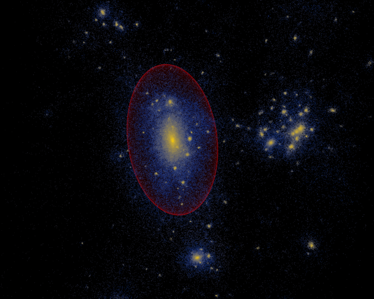
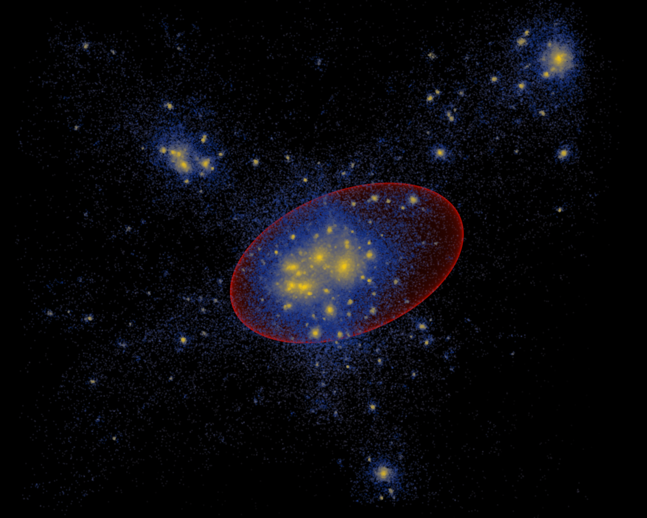
In figure 1 we show the density distribution of dark matter of two haloes (colour scale) and, in red, the computed ellipsoid which encloses an overdensity of $\delta_{vir}$. The object on the left has a virial mass of $5.29\times 10^{14}\leavevmode\nobreak\$M${}_{\odot}h^{-1}$ and represent a relaxed halo; the mass of the one on the right is $6.90\times 10^{14}\leavevmode\nobreak\$M${}_{\odot}h^{-1}$ and it is clearly multi-modal. It can be seen that the ellipsoid captures quite well the overall three-dimensional matter distribution of the relaxed halo; though it fails, as expected, with the perturbed object. For this reason we will need to eliminate from the catalogue all unrelaxed haloes like the one on the right panel. A possible way to discriminate this kind of objects is to look at the offset between centre of mass and geometrical centre of the ellipsoid. The latter is centred in the minimum of potential, which corresponds to one of the substructures; on the other hand the the centre of mass of a system like this is somewhere in between the different objects. In turn this means that if a significant number of large substructures is present, there will be an offset between the centre of the ellipsoid and the centre of mass.

2.4 Halo selection

Figure 2: Mass function and halo selection of the Millennium XXL sample at redshift $z=0$ (red squares) and $z=1$ (blue circles) obtained with the ellipsoidal overdensity. The vertical dashed line indicates the mass of an halo with $1000$ particles. Top panel: points show the mass function of the whole selected halo catalogue. It is clearly visible the cut at low masses.Bottom panel: points show the percentage of relaxed haloes in each mass bin (i.e. objects with a centre offset smaller than $5$ per cent of their virial radius.)

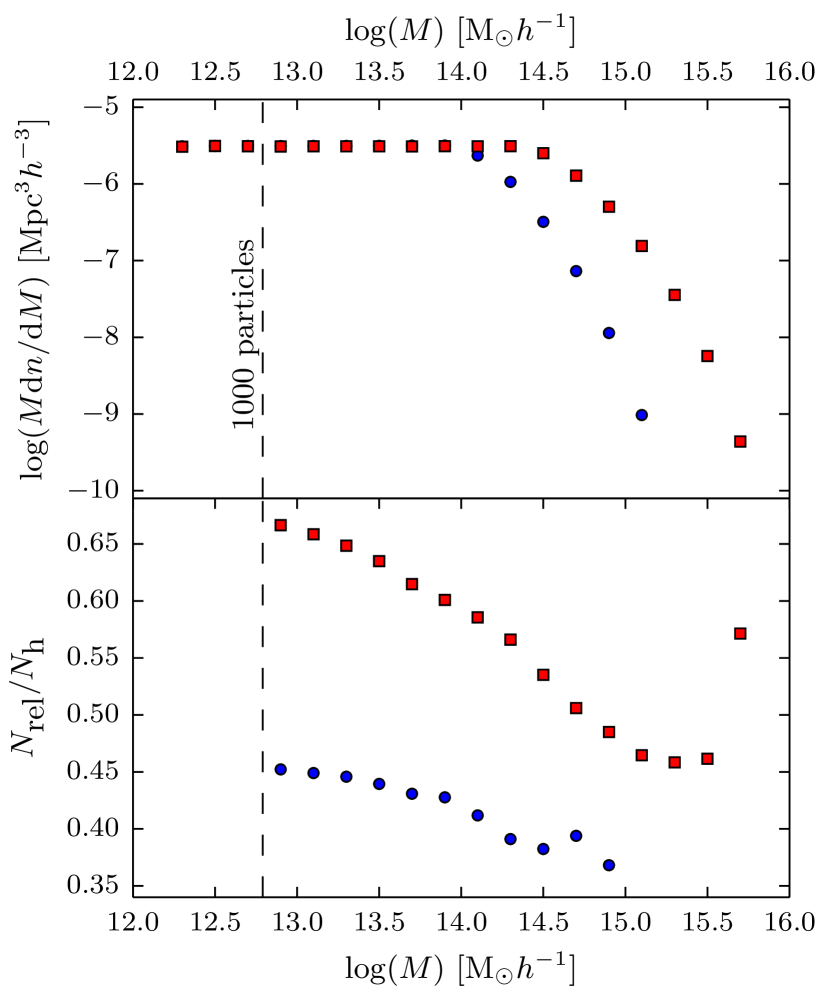
Figure 2 shows the mass function of all haloes (upper panel), which is defined as the mass within the ellipsoid that encloses an overdensity of $\Delta_{vir}$, computed by the ellipsoidal algorithm described above. Data from redshift $z=0$ and $z=1$ are indicated by red squares and blue circles respectively. As previously explained, we have analysed only a random sample of the entire halo catalogue of the MXXL simulation: this is causing the flattening at the mass bins which have more than $10^{5}$ objects in the entire box. To avoid any resolution effect, we have kept only haloes with at least $1000$ particles within the ellipsoid (vertical dashed line).

Finally, we cleaned the halo catalogue from unrelaxed haloes. An example of why this selection is necessary is the halo on the right panel of Figure 1. The object is highly asymmetrical and lacks of a well defined centre, therefore it can not be described with a single triaxial model. To remove this effect we select only haloes for which the offset between the most bound particle and the centre of mass of the particles enclosed by the ellipsoid is less than $5$ per cent of their virial radius:

$$\frac{\left|\bar{x}_{MBP}-\bar{x}_{cm}\right|}{R_{vir}}<0.05.$$ (2)

The lower panel of Figure 2 shows the percentage of cleaned haloes as a function of mass. As expected the number of perturbed haloes increases with the mass, due to more massive haloes being assembled recently. In the past (blue circles), the percentage of relaxed haloes was lower and more constant with mass, than at the present time (red squares). For cluster masses the number of relaxed haloes is roughly $50$ per cent. Although in the literature it is customary to use substructure mass fraction and virial ratio of kinetic to potential energy as measurements of the dynamical state of an halo; doing so would have required to recompute these quantities in an ellipsoidal framework. We can compare the percentage of unrelaxed haloes with Ludlow et al. (2012): using a similar selection ($N_{200}>5000$ and spherical haloes) the fraction of objects with an offset less than $5$ per cent is $0.536$, while it becomes $0.285$ combining all the three relaxation criteria. Therefore, by adopting this simplified selection we are still able to capture approximately $65$ per cent of all perturbed haloes. Moreover, configurations where the offset is small but the other two criteria fails are quite symmetrical: it is possible to properly define a centre and the triaxial approximation is applicable.

This last method for selecting the relaxed haloes has also been applied to the five SBARBINE simulations, obtaining a catalogue equivalent to the MXXL haloes. The resulting number of relaxed haloes for both simulations at redshift $z=0$ is shown in Table 1.

3 Triaxial shapes of massive galaxy clusters from MXXL

3.1 Millennium XXL results

In this first analysis we are mostly interested in the clusters mass range, therefore we will use only a portion of the available MXXL data. By taking the ratio of minor to major axis $s=a/c$ we can measure the degree of triaxiality of a halo: the closer $s$ is to $0$, the less spherical the object is. If we combine this information with the value of the intermediate to major axis ratio $q=b/c$, we can infer how much prolate or oblate the halo is.

Figure 3: Probability distribution functions – differential and cumulative – of $s=a/c$. The distributions for the entire haloes population is shown in grey (and with dashed lines), while the red (solid) ones refer to the cleaned population.

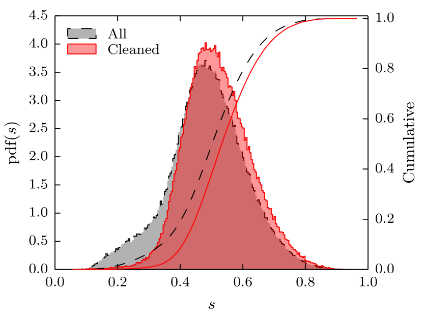
In Figure 3, the distribution of $s$ is shown for the entire halo catalogue (dashed grey curves), and for the relaxed one (solid red curves). The filled histograms represent the differential distributions, while the curves are cumulative distributions of the two different samples. In the original population there is a noticeable bump at low $s$ which corresponds to highly aspherical objects; clearly this is the case of unrelaxed or merging clusters. As it can be seen in the red histogram, the selection criteria we adopted have helped to remove this unwanted feature, since modelling them is beyond the goal of this work.

	$z=0$		$z=1$
$\log(M)[$M${}_{\odot}h^{-1}]$	$N_{h}$	$N_{rel}/N_{h}$	$N_{h}$	$N_{rel}/N_{h}$
14.0 - 14.2	57759	58.56 %	30823	41.19 %
14.2 - 14.4	56083	56.61 %	13271	39.11 %
14.4 - 14.6	42951	53.52 %	3914	38.24 %
14.6 - 14.8	20715	50.60 %	919	39.39 %
14.8 - 15.0	7823	48.50 %	134	36.81 %
15.0 - 15.2	2305	46.46 %	6	19.35 %
15.2 - 15.4	523	45.84 %
15.4 - 15.6	84	46.15 %

Table 2: Number of haloes in each logarithmic mass bin ( in $\log(M/M_{\odot}h)$ ) and percentage of relaxed haloes for redshifts $z=0$ and $z=1$.

We have divided our sample in eight logarithmic mass bins, from $10^{14}\leavevmode\nobreak\$M${}_{\odot}h^{-1}$ to $3.98\times 10^{15}\leavevmode\nobreak\$M${}_{\odot}h^{-1}$. Table 2 reports the total number of haloes $N_{h}$ and the percentage of relaxed ones $N_{rel}/N_{h}$ for each mass bin for both redshifts of the MXXL. As expected, the number of clusters at high redshift is lower and we do not have any halo in the highest mass bins. As noted before, the percentage of relaxed haloes is higher at low masses, which formed earlier and thus had more time to reach an equilibrium state.

It has already been established (Jing & Suto, 2002; Allgood et al., 2006; Bett et al., 2007; Schneider et al., 2012) that the axis ratio $s$ depends on the mass of the halo, however this dependence has not been tested at the high masses available in large simulation boxes such as the Millennium XXL.

Figure 4: Probability distribution function of $s=a/c$ binned in mass using a fixed bin of $0.2\leavevmode\nobreak\$M${}_{\odot}h^{-1}$ for both redshifts. For clarity, we show the results for only five of the mass bins reported in Table 2.

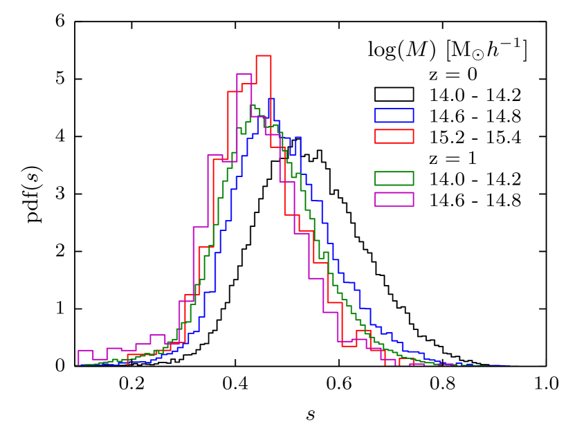
Figure 4 shows the distributions of $s$ for different masses bins in our sample – only five mass bins of Table 2, to avoid an overcrowded plot; as halo mass increases, the median value of the axis ratio becomes smaller, that is, the halo is less spherical. This effect is barely visible at redshift $z=1$. Moreover the dispersion in $s$ is larger in the lower bins. It is also noticeable that the distributions are not symmetric, particularly they are skewed to low values of the axis ratio.

Figure 5: Conditional distributions $p(q|s)$, with $q=b/c$. Different colours represent the distributions for six bins in $s$; solid and dashed histogram shows data from redshift $0$ and $1$ respectively. The vertical dashed lines of corresponding colour show the median value of $s$ for each bin.

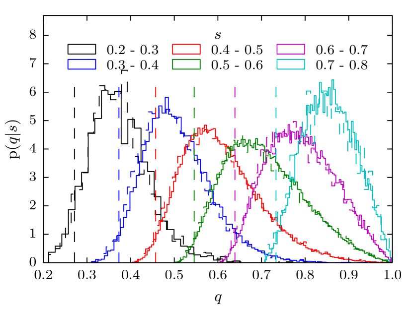
To fully describe the shape of haloes, we need also the conditional probability distribution function $p(q|s)$, which is the distribution of $q$ for a given value of $s$. Figure 5 shows the conditional distributions obtained for six bins in $s$: solid histogram for $z=0$ and dashed for $z=1$. The two redshifts are almost indistinguishable, which hints at the universality of the conditional distribution that will be discussed later on. For any interval, the median value of $b/c$ is fairly close to the median of $a/c$ (dashed vertical lines): although still fully triaxial, haloes tend to be prolate rather than oblate. For example, in the case of a “disc-like” object, all the distributions would have been prominently shifted to values close to unity, because, in this case, $b\approx c$ independently of the minor axis $a$.

3.2 Axis ratio distribution: minor to major

We aim to obtain a functional form to describe the axial ratio distributions at different masses. Due to the low statistic, Jing & Suto (2002) were not able to fully resolve the shape of the distribution and therefore assumed a Gaussian distribution. On the other hand, Schneider et al. (2012) claimed to be able to fit all the masses with a single beta distribution, although, even after a rescaling of $s$, they mention some residual mass dependence. Thanks to the high statistic in the Millennium XXL simulation we are able to reconstruct the distributions with greater detail, even at large masses. Moreover, we are only interested in clusters, so we do not need the same level of generalisation of the previous authors (see section 4 for broader analysis). These two conditions allow us to simplify the analysis and obtain a better fit of the axial ratio distributions.

As shown by various authors (Press & Schechter, 1974; Bond et al., 1991; Lacey & Cole, 1993) the mass function written as a function of peak height $\nu=\delta_{c}(z)/\sigma(M)$ does not depend on redshift nor on cosmology (see appendix A for the details on how to compute $\nu$). It is easy to understand why: $\delta_{c}(z)$ is the critical overdensity of the spherical collapse model (initial density required for a fluctuation to collapse at redshift $z$), it increases with $z$; $\sigma(M)$ is the variance in the initial density field smoothed on a scale of a uniform sphere of mass $M$ and is higher for small masses. Then, since in the past haloes were less massive, the dependences on time of the two quantities compensate with each other. For example, $\nu(M_{\star},z)=1$ at every redshift, and $\nu>1$ always represent a halo with a mass larger than the typical haloes collapsing at that time, even though the exact value of $M_{\star}$ changes with redshift.

Figure 6 shows the logarithm of the first axis ratio versus logarithm of peak height ($\approx$mass) for the selected haloes. Medians of $\log(s)$ for the two redshifts are shown in red squares and blue circles: the redshift dependence seen in fig. 4 has disappeared completely. As already shown by Despali et al. (2014, Fig. 5), the universality of haloes properties seems to extend also to the shape when using $\nu$ instead of mass. The change of variable allows us to provide results that are independent of the redshift and valid for different cosmologies. This idea was already in the original Jing & Suto (2002) paper, as the mass was given in units of $M_{*}$, but the use of $\nu$ is more general and gives a more direct connection to the theory of structure formation. As a result, we can safely treat the two datasets as a single population, shown by the box and whiskers plot for a given $\nu$ bin (horizontal error bars). This plot confirms the previously mentioned trend: more massive haloes (higher $\nu$) are more aspherical.

We have looked for a linear relation between $\nu$ and axis ratio in the log-log space, which translate to a relation similar to the rescaling adopted by previous authors: $\log\left(s\right)=a\log\left(\nu\right)+b\Rightarrow\tilde{s}=10^{b}=10^{\log s-a\log\left(\nu\right)}=s\,\nu^{-a}.$

Figure 6: (logarithmic) Distribution of $s$ as function of peak height: the black boxes and whiskers represent the quartiles and $1.5$ the quartiles range of the combined distributions. The horizontal error shows the different bins, while the green solid line is the linear fit to the medians. Red squares and blue circles are redshift $0$ and $1$ sub-samples.

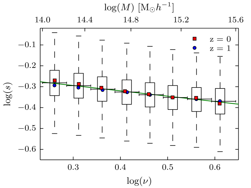
The green line is a fit of the median values; its inclination $a=-0.255\pm 0.01$ is the opposite of the exponent in the rescaling relation and the intercept is the logarithm of the median axis ratio at $M_{\star}$: $\tilde{s}(M_{\star})=10^{b}=0.61\pm 0.01$, which however does not enter directly in the following relations. The fit yields to a scaled axis ratio of:

$$\tilde{s}=s\nu^{0.255};$$ (3)

as $\nu$ takes care of any time and cosmology dependence, this rescaling is valid also for different redshifts and cosmologies.

Figure 7: Distribution of the scaled axial ratio $\tilde{s}$ for masses shown in Table 2. It can be easily seen that the distributions at all masses are well represented by an unique fitting function.

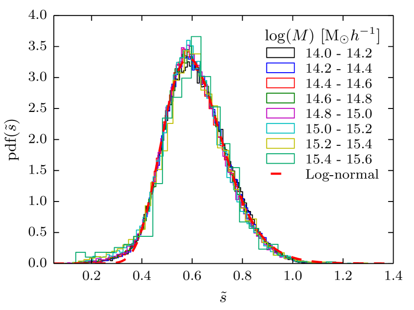
As Figure 7 shows, distributions of the rescaled axis ratios (coloured histograms) are nearly indistinguishable from each other, meaning that we have eliminated all the dependence on the mass, in contrast with the findings of Schneider et al. (2012). Moreover, we were not able to fit the histogram of $\tilde{s}$ with a beta distribution. As it can be seen in Figure 7, the distributions are non zero at values greater than $\tilde{s}=1$; this does not mean that there are haloes with axis ratio greater than $1$: $\tilde{s}$ is not a physical quantity, this effect is due to the rescaling. Nevertheless, one can argue that $\tilde{s}$ represents the physical axis ratio at $\nu=1$ ($M=5.8\times 10^{12}\leavevmode\nobreak\$M${}_{\odot}h^{-1}$); still, this rescaling has been obtained only for $M>10^{14}\leavevmode\nobreak\$M${}_{\odot}h^{-1}$, leaving the unscaled axis ratio well within the physically meaningful boundaries. We have chosen to fit the minor to major axis ratio using a log-normal distribution:

$$p(x,\mu,\sigma)=\frac{1}{x\sqrt{2\pi}\sigma}exp\left(-\frac{\left(\ln x-\mu\right)^{2}}{2\sigma^{2}}\right),$$ (4)

which corresponds to the probability distribution function of a variable which is normally distributed in the logarithmic space. The parameters of the fitted function are the following:

$$\begin{split}\mu=&-0.49\\ \sigma=&\;0.20;\end{split}$$ (5)

they can be converted to more familiar quantities:

$$\begin{split}\text{median }&=e^{\mu}=0.61,\\ \text{std }&=\sqrt{(e^{\sigma^{2}}-1)e^{2\mu+\sigma^{2}}}=0.13\;.\end{split}$$ (6)

In this framework, for a simple analysis, one can just use the scaled median value $\tilde{s}=0.61$ with asymmetric quartiles at $0.53$ and $0.70$; then use eq. (3) to obtain the physical value: $s=\tilde{s}\left(\nu\right)^{-0.255}$. On the other hand, it is possible to use the fit to obtain the whole distribution for a given mass. For example, to use it as a prior distribution of the minor to major axis ratio, one draws a value $x$ from a normal (Gaussian) distribution with mean $\mu=-0.49$ and standard deviation $\sigma=0.20$, the scaled axis ratio is then $e^{x}$ (or directly extract $\tilde{s}$ from a lognormal distribution); inverting the rescaling relation one can obtain the axis ratio of the halo at a given peak height, which can be subsequently converted in mass for a given cosmology at a given redshift.

3.3 Axis ratio distribution: intermediate to major

Once we are able to describe $s$ as a function of mass we can look at the correlation between the two axial ratios. For construction, $q$ is always greater (or equal) than $s$; also it is always less than $1$. These limits have the effect of distorting the distribution of intermediate to major axis ratio in a way that depends directly on $s$.

Figure 8: Distribution of $\tilde{q}=(q-s)/(1-s)$ as function of $s$: the black boxes and whiskers represent the quartiles and $1.5$ the quartiles range respectively. The horizontal red error bars represent the bin inside which the medians have been computed. $Right$ : Distributions of $\tilde{q}$ for different values of $s$ (histograms) and fitting function resulting from the model presented in the section (curves).

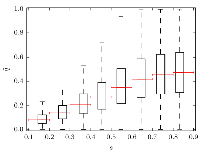
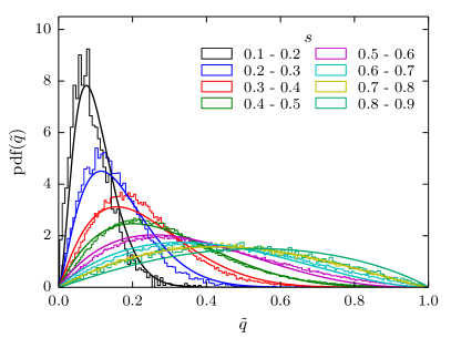
To avoid this problem we use the rescaled quantity $\tilde{q}=(q-s)/(1-s)$ instead of the simple axial ratio (Schneider et al., 2012), eliminating the issues of a limited interval; the correlation between the rescaled second axial ratio and $s$ can be seen in the left panel of Figure 8, where are shown medians (red error bars) and quartiles (box and whiskers plot) for different values of the first axis ratio. We have divided $\tilde{q}$ in bins of different $s$ and extracted the distributions $p(\tilde{q}|s)$ (right panel of Fig. 8). From both plots, it is quite evident that $\tilde{q}$ strongly depends on the first axial ratio, with higher values at higher $s$, which is in agreement with haloes that tend to be prolate. Moreover the scatter is larger at higher $s$, though this is mostly due to the rescaling which extends the allowed interval of $\tilde{q}$.

Because of the strong correlation between $\tilde{q}$ and $s$, we can not just give $\tilde{q}$ as a function of mass: to obtain the second axis ratio distribution for a given mass, we have to describe $p(\tilde{q}|s)$ and then get the first axis ratio from its distribution at different masses (as shown in Section 3.2). Given the large differences in the shapes of the distributions of $\tilde{q}$ at a given $s$, the rescaling needed to reduce them to a single one needs to be much more complex than the one adopted in the last section. Therefore, we fit each single histogram with a different beta distribution, which has the following analytical expression:

$$p(x,\alpha,\beta)=\frac{1}{B(\alpha,\beta)}x^{\alpha-1}(1-x)^{\beta-1}.$$ (7)

This function has two shape parameters $\alpha$ and $\beta$; the factor $1/B(\alpha,\beta)$ is a normalisation constant that can be computed by requiring that the integral of the probability distribution function is equal to unity.

From the fitting procedure we obtained a pair of parameters for each bin in $s$; however $\alpha$ has a complicated dependence on the first axial ratio (almost constant with an average value of $\alpha=2.15$), while the mean value of the beta distributions $\mu=1/(1+\beta/\alpha)$ follows a linear relation.

Figure 9: Parameters of the fitted beta functions. Red is the mean of the distribution, in blue the second parameter $\beta$.

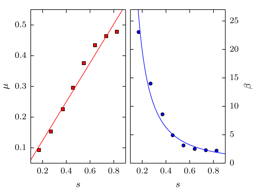
Figure 9 shows the dependence of the mean $\mu$ (red squares on left panel) and $\beta$ parameter (blue circles on right panel) of the fitted beta functions on the first axial ratio $s$. The coloured lines in each respective panel show a fit of these two parameters:

$$\begin{split}\mu(s)&=0.633s-0.007\\ \beta(s)&=1.389s^{-1.685}.\end{split}$$ (8)

These two equations give us a functional form of $p(\tilde{q}|s)$: starting from a value of $s$, one can retrieve the mean $\mu$ and $\beta$ from which the other parameter can be computed $\alpha=\beta/(1/\mu+1)$. This gives what is needed to reconstruct the distribution of $\tilde{q}$ of a given $s$ and the scatter, if needed. The final step is to revert the change of coordinates and compute the physical axial ratio $q$.

4 Exploding the mass range to 5 orders of magnitude

The next step of our work is to explode the recipes for dark matter halo shapes to lower masses: in the following sections we describe how to generalise the axial ratio distribution to a wider mass range. To do so, we combined the MXXL data with the SBARBINE simulations, a set of cosmological simulations that will allow us to study the shape of dark matter haloes from $3\times 10^{10}\leavevmode\nobreak\$M${}_{\odot}h^{-1}$ to $6\times 10^{15}\leavevmode\nobreak\$M${}_{\odot}h^{-1}$.

As before, we express the mass dependence in terms of peak height $\nu$. By doing this, it is possible to treat homogeneously data from different redshifts and cosmologies, such as the SBARBINE and the MXXL simulations.

4.1 Axis ratio distribution: minor to major

Figure 10: $Left$: Distribution of $s$ as function of peak height for all the haloes selected from both redshifts the two simulations: the black boxes and whiskers represent the quartiles and $1.5$ the quartiles range respectively computed within the bins shown by the horizontal error bars. The coloured points represent the medians for individual redshifts for the two simulations. $Right$ : Differential distribution of $s$ for 8 bin in $\nu$ (histograms) and the respective approximating functions obtained as shown in the section (curves).

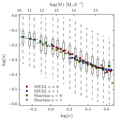
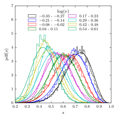
On left panel of figure 10, the logarithm of the minor to major axial ratio $s$ is shown as a function of the logarithm of $\nu$. As before, horizontal error bars represent the interval in $\nu$ and the box and whiskers are the quartiles and 1.5 the quartiles range for the combined sample, while coloured points are medians of individual catalogues. Again, there is no difference in the medians between redshifts, neither between the single simulations. It can be seen that $s$ has a nearly linear dependence on $\log(\nu)$, with a hint of flattening at both high and low masses.

For each bin, we extracted the probability distribution function of $\log(s)$ (right panel of Fig. 10). The resulting curves exhibit an interesting pattern: high and low $\nu$ histograms are mirrored with respect to a central symmetric distribution which corresponds to $\nu=1.21$ ($M\approx M_{*}$). The rescaling adopted in section 3.2 does not compensate this large variation in the form of the distributions and it is not able to remove entirely the mass dependence. Instead of using a different rescaling relation to obtain a single pdf, we decided to follow the same recipe we used for the second axial ratio: first of all we separately fit each distribution and then we relate the resulting parameters to the binning quantity.

Figure 11: Parameters of the fitted beta functions. Red is the mean of the distribution, in blue the second parameter $\beta$.

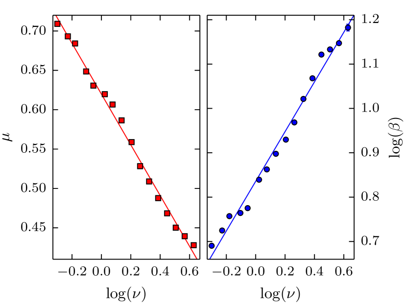
This is shown in Figure 11, where we fit the mean (left panel) and $\beta$ parameter (right panel) of the Beta distributions we derived by fitting the histograms of the right panel of Fig. 10. In order to keep the procedure simple we fit with a linear relation both $\mu$ and $\log\beta$:

$$\begin{split}\mu(\nu)&=-0.322\log\nu+0.620\\ \log\left(\beta(\nu)\right)&=0.560\log\nu+0.836.\end{split}$$ (9)

As before, the dependence of $\alpha$ is difficult to describe and it is almost constant with a value of about $11.21$.

Using this fits we are now able to approximate the probability distribution function of the first axial ratio with a Beta function with parameters $\alpha=\beta/(1/\mu-1)$ and $\beta$, over a range in mass of almost $6$ orders of magnitudes. Moreover the use of $\nu$ allows us to extend these results to different cosmologies and different redshifts.

4.2 Axis ratio distribution: intermediate to major

Figure 12: Axis ratio $q$ as function of $s$ for different masses, represented by the points of different colours. Since there is no residual mass dependence in the conditional distribution, we get the same result as in the MXXL with all the simulations, confirming that this relation is universal.

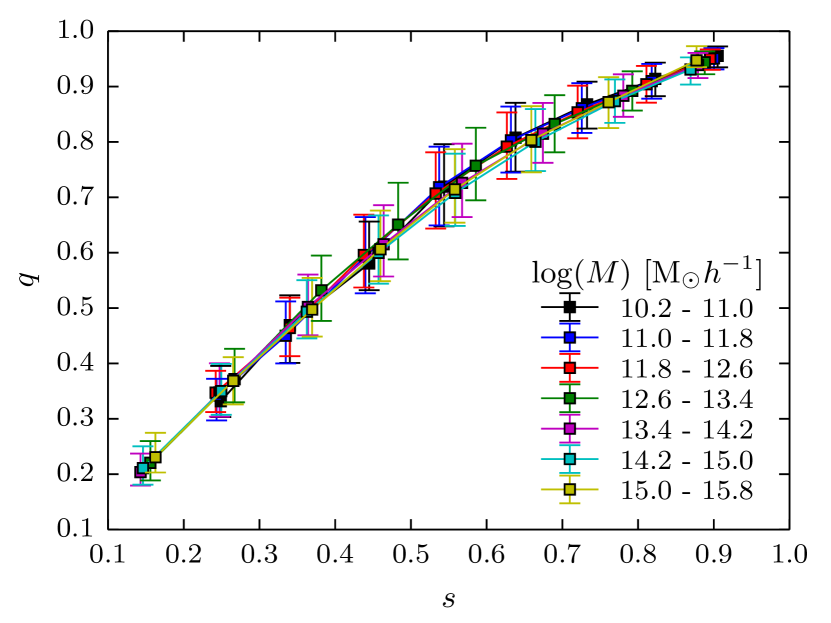
Finally, to fully describe a triaxial halo of a given mass the intermediate to major axis ratio has to be parametrized. As Figure 12 shows, the relation between $q$ and $s$ at redshift $z=0$ does not depend on the mass: the curves of different colours represent different mass bins and still trace the same relation. The fact that all the mass dependence is already inside $s$, allows us to use for $p(q|s)$ the same functional form of section 3.3, independently of the mass we choose. The same applies to different redshifts (not shown here, but see 5 for a limited comparison), with the relation between the two quantities being indistinguishable from the one in Fig. 12. Moreover, this independence of the conditional distribution from both mass and redshift is in agreement with the theoretical predictions from Rossi et al. (2011).

5 Comparison with previous works

Figure 13: Comparison between previous works (dashed lines) and the results of this paper (solid lines). Red squares represent the data from both redshifts of the MXXL and the SBARBINE simulations, converted to redshift $z=0$ for the Millennium cosmology. The blue solid line is the model for clusters shown in section 3.2; the green solid line is the fit for the entire mass interval from section 4.1. The dotted parts of the curves show the mass ranges outside where the relations have been derived from.

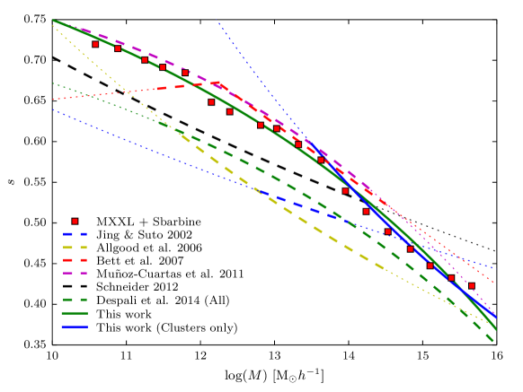
We have compared our results with measurement of axis ratios from other authors (Fig. 13). The data from both redshifts of the Millennium XXL and SBARBINE simulations are shown with red squares, the median result form the analysis on cluster masses (sec. 3.2) is the blue solid line and the green solid line is from the combined datasets (sec. 4.1). Results from other authors are shown with dashed lines in the mass range where their analysis was carried out and with dotted lines when extrapolated beyond it. Moreover all data and predictions have been converted to redshift $z=0$ for the Millennium cosmology, when necessary. As it can be seen, there is a general agreement in the dependence of $s$ on the mass, with more massive haloes being less spherical. Although there seems to be a scatter of about $15$ per cent, this is due more to the differences in the method of measuring shapes (different finders, radius, cleaning procedure), than an error on the measurement. It must be noticed that instead of the spherical mass, we used the mass within the ellipsoid for consistency reasons; yet, this does not substantially alter the findings presented here.

The most important difference comes from the radius at which the shape is measured. Jing & Suto (2002) (blue dashed line) used particles of the isodensity surface corresponding to $2500\delta_{c}$, roughly at a radius of $0.3R_{\text{vir}}$; this analysis is different from all the following authors, as it reflects the shape of an ellipsoidal shell, and not of all the mass inside the ellipsoid. Their mass range $6\times 10^{12}$ – $10^{14}\leavevmode\nobreak\$M${}_{\odot}h^{-1}$ was also quite small compared to later analysis.

Studying a larger mass interval, $6\times 10^{11}$ – $3\times 10^{14}\leavevmode\nobreak\$M${}_{\odot}h^{-1}$, Allgood et al. (2006) (yellow dashed line) derived axis ratios of particles distribution inside $0.3R_{\text{vir}}$ diagonalizing the normalised mass tensor (weighted by the distance from the centre); because of this their measure reflects the shape at a even closer radius.

On the other hand, Schneider et al. (2012) (black dashed line) extended the analysis up to the virial radius, nevertheless the use of the normalised tensor prevents a meaningful comparison with our results.

All of these results are lower than what we derived, which can be explained by the fact that the shapes were measured at inner radii, where the particle distribution is supposed to be more elongate . However, if we restrict the comparison to works that used particles within the virial radius the agreement becomes much more strong. This is the case of Muñoz-Cuartas et al. (2011) (magenta dashed line), who studied shapes with an ellipsoidal overdensity algorithm similar to the one adopted in this work: their results agree with ours much more than any other work.

Finally, using a different type of halo finder, Bett et al. (2007) (red dashed line) measured $s$ for a set of particles that represent all the bounded particles of an halo without assuming any particular shape; the finder also clean the sample for unrelaxed haloes. The agreement with our results is another indication that an ellipsoid is a good approximation for relaxed haloes.

The other difference can arise from the cleaning of the sample; the green dashed line show the prediction from Despali et al. (2014), which is obtained from all haloes, regardless of their state of relaxation. As expected the values are lower, since unrelaxed haloes are typically irregular and so they appear more elongated with lower axial ratios. The difference is greater for less massive haloes.

6 Summary and Conclusions

We have studied the triaxiality of dark matter haloes from the Millennium XXL Simulation, which enabled us to characterise the shape of haloes with extremely good statistic in the galaxy clusters mass range, from $10^{14}\leavevmode\nobreak\$M${}_{\odot}h^{-1}$ to $4\times 10^{15}\leavevmode\nobreak\$M${}_{\odot}h^{-1}$. Using the SBARBINE simulations, we have extended our analysis to lower masses down to $3\times 10^{10}\leavevmode\nobreak\$M${}_{\odot}h^{-1}$, thus increased the mass range by more than 5 orders of magnitude. The main results of our analysis are the following:

• dark matter haloes are triaxial with a tendency of being prolate and in particular more massive objects are less spherical; as shown in Fig. 3 unrelaxed haloes have the effect of artificially increasing the axis ratios and can not be described by this simple ellipsoidal model, which is unimodal by construction;

• for clusters, the distribution of the rescaled minor to major axis ratio is well described by a lognormal distribution, in contrast to previous extrapolations from lower masses that found a simple Gaussian fit;

• over the whole examined mass range, $s$ can be approximated by a beta distribution that depends only on the peak height $\nu$;

• the conditional intermediate to major axis ratio distribution $p(q|s)$ can also be described by a beta distribution that depends only on the first axis ratio and not on the mass, thus the same approach can be used for both clusters and the whole mass range of haloes;

• overall, the probability distribution function of the shape of a dark matter halo is given by one single parameter $\nu$, related to its mass, that incorporates the dependence on redshift and cosmology. This goes in support of methods that allows to change the cosmology of a numerical simulation (Angulo & White, 2010), as within good approximation most of halo properties depend only on $\nu$.

In the recipe that we provide, an halo shape is determined only by its mass and can be changed to different cosmologies and redshifts. Depending on the level of precision desired, it is possible to choose different approximations:

• for a simpler analysis that is focused on the entire mass range, section 4.1 presents a single method that can be applied to masses from $10^{10}$ up to $10^{16}\leavevmode\nobreak\$M${}_{\odot}h^{-1}$. If restricted to masses lower than $10^{14}\leavevmode\nobreak\$M${}_{\odot}h^{-1}$, this is actually a very accurate description of haloes shapes;

• if the interest is only on clusters shapes, then section 3.2 gives a more precise model;

• finally, it is possible to combine the two description and just use the most suitable one given the mass of the halo, although losing the universality of the description.

A simple implementation of this model can be found on a dedicated website.

In section 5 we have compared our results with previous findings. There is a general agreement with previous works within a $15$ per cent scatter that is due to the different methods used and especially to the radius at which the shape is measured. However, the picture is clear: dark matter haloes are triaxial objects and this effect is more prominent in clusters where the spherical model is quite far from being able to realistically represent the matter distribution.

Appendix A Density peak height

In this appendix we describe step by step how to compute density peak height $\nu$ for a virialized halo with mass $M$ at redshift $z$ for a given cosmological model. Its definition is the following:

$$\nu\equiv\frac{\delta_{c}(z)}{\sigma(M)},$$ (10)

where $\delta_{c}(z)$ is the critical overdensity of the spherical collapse model, the initial density required for a fluctuation to collapse at redshift $z$. This in turn can be expressed as the collapse overdensity at redshift $z=0$ rescaled to a given time: $\delta_{c}(z)=\delta_{c}/D(z)$, with $D(z)$ being the linear growth rate of a density fluctuation normalised to unity at the present time. The overdensity $\delta_{c}$ depends only on redshift and not on the mass; on the other hand, the denominator $\sigma(M)$, depends on the mass but not on redshift. It is the variance in the initial density field smoothed on a linear scale $R$, which corresponds to the radius of a uniform sphere of mass $M$. Therefore, only the linear growth rate $D(z)$ and the initial power spectrum $P(k)$ are needed.

From the linear perturbation theory, it is possible to compute $D(z)$:

$$D(z)\propto H(t)\int_{0}^{t}\frac{\text{d}t^{\prime}}{a^{2}(t^{\prime})H^{2}(t^{\prime})},$$ (11)

which has to be solved numerically. Fortunately, there is an approximated solution (Carroll et al., 1992) that can be expressed as $D(z)\propto g(z)/(1+z)$, where:

$$g(z)=\frac{5/2\,\Omega_{m}(z)}{\Omega_{m}^{4/7}-\Omega_{\Lambda}(z)+\left[1+\Omega_{m}(z)/2\right]\left[1+\Omega_{\Lambda}(z)/70\right]}.$$ (12)

Additionally, the collapse overdensity has an extremely weak dependence on cosmology: $\delta_{c}\approx 1.686\left[\Omega_{m}(t_{c})\right]^{0.0055}$; for realistic cosmologies this can be approximated to $\delta_{c}\approx 1.69$. Therefore, at the present time the collapse overdensity is $\delta_{c}$ and it increases with redshift, due to $D(z)$.

The other quantity required, the variance $\sigma^{2}(M)$, is defined from the power spectrum as:

$$\sigma^{2}(M)=\frac{1}{2\pi^{2}}\int_{0}^{\infty}P(k)\tilde{W}^{2}(kR)k^{2}\text{d}k;$$ (13)

where $\tilde{W}$ is the Fourier transform of a window function. Typically, $W$ is a Top Hat (sphere) in the coordinates space, so that its Fourier transform $\tilde{W}$ is:

$$\tilde{W}(kR)=3\frac{\sin\left(kR\right)-kR\cos\left(kR\right)}{\left(kR\right)^{3}};$$ (14)

with the radius $R$ given by $M=\rho_{b}4\pi/3R^{3}$. The power spectrum $P(k)$ of the density fluctuations is the main input; given a set of cosmological parameters it can be computed from a software like CAMB (Lewis et al., 2008). As it is function of initial conditions only, $\sigma(M)$ needs to be computed only once for a given cosmology: all the redshift dependence is inside $D(z)$.

Finally, for an halo of mass $M$, using eq. (13) it is possible to compute $\sigma(M)$ and combine it with the value of $D(z)$ from eq. (12) to obtain the correct density peak height $\nu$.

References

- Allgood et al. (2006) Allgood B., Flores R. A., Primack J. R., Kravtsov A. V., Wechsler R. H., Faltenbacher A., Bullock J. S., 2006, MNRAS, 367, 1781
- Allgood et al. (2006) Allgood B., Flores R. a., Primack J. R., Kravtsov a. V., Wechsler R. H., Faltenbacher a., Bullock J. S., 2006, MNRAS, 367, 1781
- Angulo et al. (2012) Angulo R. E., Springel V., White S. D. M., Jenkins a., Baugh C. M., Frenk C. S., 2012, MNRAS, 426, 2046
- Angulo & White (2010) Angulo R. E., White S. D. M., 2010, MNRAS, 405, 143
- Bailin & Steinmetz (2005) Bailin J., Steinmetz M., 2005, ApJ, 627, 647
- Bett et al. (2007) Bett P., Eke V., Frenk C. S., Jenkins A., Helly J., Navarro J., 2007, MNRAS, 376, 215
- Binggeli (1982) Binggeli B., 1982, A&A, 107, 338
- Bond et al. (1991) Bond J. R., Cole S., Efstathiou G., Kaiser N., 1991, The Astrophysical Journal, 379, 440
- Boylan-Kolchin et al. (2009) Boylan-Kolchin M., Springel V., White S. D. M., Jenkins A., Lemson G., 2009, MNRAS, 398, 1150
- Buote & Canizares (1992) Buote D. A., Canizares C. R., 1992, ApJ, 400, 385
- Buote & Canizares (1996) Buote D. A., Canizares C. R., 1996, ApJ, 457, 565
- Carroll et al. (1992) Carroll S. M., Press W. H., Turner E. L., 1992, ARA&A, 30, 499
- Carter & Metcalfe (1980) Carter D., Metcalfe N., 1980, MNRAS, 191, 325
- Cole & Lacey (1996) Cole S., Lacey C., 1996, MNRAS, 281, 716
- Despali et al. (2014) Despali G., Giocoli C., Tormen G., 2014, arXiv preprint arXiv:1404.6527, 11, 1
- Despali et al. (2013) Despali G., Tormen G., Sheth R. K., 2013, MNRAS, 431, 1143
- Doroshkevich (1970) Doroshkevich A. G., 1970, Astrophysics, 6, 320
- Dubinski & Carlberg (1991) Dubinski J., Carlberg R. G., 1991, ApJ, 378, 496
- Eke et al. (1996) Eke V. R., Cole S., Frenk C. S., 1996, MNRAS, 282, 263
- Evans & Bridle (2009) Evans A. K. D., Bridle S., 2009, ApJ, 695, 1446
- Fabricant et al. (1984) Fabricant D., Rybicki G., Gorenstein P., 1984, ApJ, 286, 186
- Frenk et al. (1988) Frenk C. S., White S. D. M., Davis M., Efstathiou G., 1988, ApJ, 327, 507
- Gao et al. (2012) Gao L., Navarro J. F., Frenk C. S., Jenkins A., Springel V., White S. D. M., 2012, MNRAS, 425, 2169
- Giocoli et al. (2012a) Giocoli C., Meneghetti M., Bartelmann M., Moscardini L., Boldrin M., 2012, MNRAS, 421, 3343
- Giocoli et al. (2012b) Giocoli C., Meneghetti M., Ettori S., Moscardini L., 2012, MNRAS, 426, 1558
- Giocoli et al. (2008) Giocoli C., Tormen G., van den Bosch F. C., 2008, MNRAS, 386, 2135
- Hopkins et al. (2005) Hopkins P. F., Bahcall N. A., Bode P., 2005, ApJ, 618, 1
- Jing & Suto (2002) Jing Y., Suto Y., 2002, The Astrophysical Journal, pp 538–553
- Jing & Fang (1994) Jing Y.-P., Fang L.-Z., 1994, The Astrophysical Journal, 432, 438
- Kasun & Evrard (2005) Kasun S. F., Evrard A. E., 2005, ApJ, 629, 781
- Kawahara (2010) Kawahara H., 2010, ApJ, 719, 1926
- Lacey & Cole (1993) Lacey C., Cole S., 1993, MNRAS
- Lau et al. (2012) Lau E. T., Nagai D., Kravtsov A. V., Vikhlinin A., Zentner A. R., 2012, ArXiv e-prints
- Lewis et al. (2008) Lewis A., Challinor A., Lasenby A., 2008, Astrophys. J, 2, 2
- Limousin et al. (2013) Limousin M., Morandi A., Sereno M., Meneghetti M., Ettori S., Bartelmann M., Verdugo T., 2013, Space Science Reviews, 177, 155
- Ludlow et al. (2012) Ludlow A. D., Navarro J. F., Li M., Angulo R. E., Boylan-Kolchin M., Bett P. E., 2012, MNRAS, 427, 1322
- Muñoz-Cuartas et al. (2011) Muñoz-Cuartas J. C., Macciò A. V., Gottlöber S., Dutton A. A., 2011, MNRAS, 411, 584
- Oguri et al. (2012) Oguri M., Bayliss M. B., Dahle H., Sharon K., Gladders M. D., Natarajan P., Hennawi J. F., Koester B. P., 2012, MNRAS, 420, 3213
- Oguri et al. (2010) Oguri M., Takada M., Okabe N., Smith G. P., 2010, MNRAS, 405, 2215
- Paz et al. (2006) Paz D. J., Lambas D. G., Padilla N., Merchán M., 2006, MNRAS, 366, 1503
- Planck Collaboration: et al. (2013) Planck Collaboration: Aghanim N., Arnaud M., Ashdown M., Aumont J., Baccigalupi C., Banday A. J., Al. E., 2013, arXiv preprint arXiv: …, pp 1–69
- Press & Schechter (1974) Press W. H., Schechter P., , 1974, Formation of Galaxies and Clusters of Galaxies by Self-Similar Gravitational Condensation
- Rossi et al. (2011) Rossi G., Sheth R. K., Tormen G., 2011, MNRAS, 416, 248
- Sayers et al. (011a) Sayers J., Golwala S. R., Ameglio S., Pierpa oli E., 2011a, ApJ, 728, 39
- Schneider et al. (2012) Schneider M. D., Frenk C. S., Cole S., 2012, Journal of Cosmology and Astroparticle Physics, 2012, 030
- Skielboe et al. (2012) Skielboe A., Wojtak R., Pedersen K., Rozo E., Rykoff E. S., 2012, ArXiv e-prints
- Soucail et al. (1987) Soucail G., Fort B., Mellier Y., Picat J. P., 1987, A&A, 172, L14
- Springel (2005) Springel V., 2005, MNRAS, 364, 1105
- Tormen et al. (2004) Tormen G., Moscardini L., Yoshida N., 2004, MNRAS, 350, 1397
- van Daalen et al. (2012) van Daalen M. P., Angulo R. E., White S. D. M., 2012, MNRAS, 424, 2954
- Warren et al. (1992) Warren M. S., Quinn P. J., Salmon J. K., Zurek W. H., 1992, ApJ, 399, 405