Block Renormalization for quantum Ising models in dimension d=2𝑑2d=2 :
applications to the pure and random ferromagnet, and to the spin-glass

CΓ©cile Monthus Institut de Physique ThΓ©orique, CNRS and CEA Saclay, 91191 Gif-sur-Yvette cedex, France
Abstract

For the quantum Ising chain, the self-dual block renormalization procedure of Fernandez-Pacheco [Phys. Rev. D 19, 3173 (1979)] is known to reproduce exactly the location of the zero-temperature critical point and the correlation length exponent Ξ½=1𝜈1\nu=1. Recently, Miyazaki and Nishimori [Phys. Rev. E 87, 032154 (2013)] have proposed to study the disordered quantum Ising model in dimensions d>1𝑑1d>1 by applying the Fernandez-Pacheco procedure successively in each direction. To avoid the inequivalence of directions of their approach, we propose here an alternative procedure where the d𝑑d directions are treated on the same footing. For the pure model, this leads to the correlation length exponents ν≃0.625similar-to-or-equals𝜈0.625\nu\simeq 0.625 in d=2𝑑2d=2 (to be compared with the 3D classical Ising model exponent ν≃0.63similar-to-or-equals𝜈0.63\nu\simeq 0.63) and ν≃0.5018similar-to-or-equals𝜈0.5018\nu\simeq 0.5018 (to be compared with the 4D classical Ising model mean-field exponent Ξ½=1/2𝜈12\nu=1/2). For the disordered model in dimension d=2𝑑2d=2, either ferromagnetic or spin-glass, the numerical application of the renormalization rules to samples of linear size L=4096𝐿4096L=4096 yields that the transition is governed by an Infinite Disorder Fixed Point, with the activated exponent Οˆβ‰ƒ0.65similar-to-or-equalsπœ“0.65\psi\simeq 0.65, the typical correlation exponent Ξ½t​y​p≃0.44similar-to-or-equalssubscriptπœˆπ‘‘π‘¦π‘0.44\nu_{typ}\simeq 0.44 and the finite-size correlation exponent Ξ½F​S≃1.25similar-to-or-equalssubscriptπœˆπΉπ‘†1.25\nu_{FS}\simeq 1.25. We discuss the similarities and differences with the Strong Disorder Renormalization results.

I Introduction

The quantum Ising model defined in terms of Pauli matrices (Οƒix,Οƒiz)superscriptsubscriptπœŽπ‘–π‘₯superscriptsubscriptπœŽπ‘–π‘§(\sigma_{i}^{x},\sigma_{i}^{z})

H=βˆ’βˆ‘ihi​σixβˆ’βˆ‘<i,j>Ji,j​σiz​σjz𝐻subscript𝑖subscriptβ„Žπ‘–subscriptsuperscript𝜎π‘₯𝑖subscriptabsent𝑖𝑗absentsubscript𝐽𝑖𝑗superscriptsubscriptπœŽπ‘–π‘§subscriptsuperscriptπœŽπ‘§π‘—\displaystyle H=-\sum_{i}h_{i}\sigma^{x}_{i}-\sum_{<i,j>}J_{i,j}\sigma_{i}^{z}\sigma^{z}_{j} (1)

is the basic model to study quantum phase transitions at zero-temperature [1]. On a hypercubic lattice in dimension d𝑑d, the pure model with the same transverse field hβ„Žh on all sites, and the same ferromagnetic coupling J𝐽J between nearest-neighbors is well understood via the equivalence with the classical Ising model in dimension dc​l​a​s​s=d+1superscriptπ‘‘π‘π‘™π‘Žπ‘ π‘ π‘‘1d^{class}=d+1, i.e. the time plays the role of an extra space-dimension [1], and the dynamical exponent is zp​u​r​e=1subscriptπ‘§π‘π‘’π‘Ÿπ‘’1z_{pure}=1. In particular, the quantum model in d=1𝑑1d=1 corresponds to the exactly solved 2D classical Ising model, the quantum model in d=2𝑑2d=2 corresponds to the 3D classical Ising model, and the quantum model in dimension dβ‰₯3𝑑3d\geq 3 is characterized by the standard mean-field exponents.

From the point of view of Block-Renormalization for quantum models, there exists a special self-dual procedure introduced by Fernandez-Pacheco [2, 3], which is able to reproduce the exact critical point (J/h)c=1subscriptπ½β„Žπ‘1(J/h)_{c}=1 and the exact correlation length exponent ν​(d=1)=ν​(dc​l​a​s​s=2)=1πœˆπ‘‘1𝜈superscriptπ‘‘π‘π‘™π‘Žπ‘ π‘ 21\nu(d=1)=\nu(d^{class}=2)=1. Various generalizations of this procedure to higher dimensions d>1𝑑1d>1 have been studied [4, 5, 6], as well as extensions to other quantum models like the Potts and the Ashkin-Teller models [7, 8, 9, 10].

In the disordered case, where the transverse fields hisubscriptβ„Žπ‘–h_{i} and the couplings Ji,jsubscript𝐽𝑖𝑗J_{i,j} are random variables, many exact results have been obtained in d=1𝑑1d=1 by Daniel Fisher [11] via the asymptotically exact strong disorder renormalization procedure (for a review, see [12]). In particular, the transition is governed by an Infinite Disorder Fixed Point and presents unconventional scaling laws with respect to the pure case. In dimension d>1𝑑1d>1, the strong disorder renormalization procedure has been studied numerically with the conclusion that the transition is also governed by an Infinite-Disorder fixed point in dimensions d=2,3,4𝑑234d=2,3,4 [14, 13, 15, 16, 17, 18, 19, 20, 21, 22, 23]. These numerical renormalization results are in agreement with the results of independent quantum Monte-Carlo in d=2𝑑2d=2 [24, 25]. The Strong Disorder Renormalization is thus a very powerful method, but it leads to a complicated renormalized topology for the surviving clusters as soon as d>1𝑑1d>1. In particular, a large number of very weak bonds are a priori generated during the RG, that will eventually not be important for the forthcoming RG steps. This is why recent numerical implementations of Strong Disorder RG rules are based on algorithms avoiding this proliferation of weak generated bonds [20, 21, 22, 23].

A natural question is whether Infinite Disorder Fixed Points can be also reproduced by more standard block-renormalization. Recently, Miyazaki and Nishimori [26] have proposed to generalize the block-renormalization of Fernandez-Pacheco [2] concerning the pure model in d=1𝑑1d=1, and their extension for the pure model in d=2,3𝑑23d=2,3 [5] to the random case : their results are in agreement with the Infinite Disorder Fixed Point scalings. However in dimension d>1𝑑1d>1, their procedure has the drawback that the various directions are treated inequivalently, so that they need to re-symmetrize afterward [5]. In addition, in the random case, they have used some pool method that does not keep all the generated correlations between renormalized parameters, and the only critical exponent that they measure is the finite-size correlation length exponent ν𝜈\nu, whereas it is interesting to measure also the activated exponent Οˆπœ“\psi and the typical correlation length exponent Ξ½t​y​p.subscriptπœˆπ‘‘π‘¦π‘\nu_{typ}.

In the present paper, we thus propose another generalization in dimensions d=2𝑑2d=2 and d=3𝑑3d=3 of the self-dual one-dimensional block-renormalization of Fernandez-Pacheco, that we study analytically in the pure case and numerically in the disordered case. The paper is organized as follows. In section II, we describe the elementary renormalization rule that will be applied throughout the paper. The application to the one-dimensional quantum Ising model of Eq. 1, both pure and random, is recalled in section III. In section IV, we derive the Block Renormalization rules for the two-dimensional case. The applications of these two-dimensional rules are discussed respectively in section V for the pure ferromagnetic model, in section VI for the random ferromagnetic model, and in section VII for the spin-glass model. Our conclusions are summarized in section VIII. The extension to dimension d=3𝑑3d=3 is presented in Appendix A.

II Elementary renormalization rule

In this section, we consider the following elementary Hamiltonian involving (b+1)𝑏1(b+1) spins ΟƒisubscriptπœŽπ‘–\sigma_{i} with i=0,1,2,..,bi=0,1,2,..,b

Hb=βˆ‘i=1b(βˆ’hi​σixβˆ’J0,i​σ0z​σiz)subscript𝐻𝑏superscriptsubscript𝑖1𝑏subscriptβ„Žπ‘–subscriptsuperscript𝜎π‘₯𝑖subscript𝐽0𝑖superscriptsubscript𝜎0𝑧subscriptsuperscriptπœŽπ‘§π‘–\displaystyle H_{b}=\sum_{i=1}^{b}\left(-h_{i}\sigma^{x}_{i}-J_{0,i}\sigma_{0}^{z}\sigma^{z}_{i}\right) (2)

where Οƒ0subscript𝜎0\sigma_{0} plays the special role of the ’master’, and the b𝑏b spins ΟƒisubscriptπœŽπ‘–\sigma_{i} with i=1,2,..,bi=1,2,..,b are the ’slaves’.

II.1 Diagonalization of Hbsubscript𝐻𝑏H_{b}

For each eigenvalue S0=Β±1subscript𝑆0plus-or-minus1S_{0}=\pm 1 of Οƒ0zsuperscriptsubscript𝜎0𝑧\sigma_{0}^{z}, one has to diagonalize independently the b𝑏b Hamiltonians concerning the single quantum spin ΟƒisubscriptπœŽπ‘–\sigma_{i} in the transverse field hisubscriptβ„Žπ‘–h_{i} and in the effective magnetic field (J0,i​S0)subscript𝐽0𝑖subscript𝑆0(J_{0,i}S_{0})

hi(S0)=βˆ’hi​σixβˆ’J0,i​S0​σizsubscriptsuperscriptβ„Žsubscript𝑆0𝑖subscriptβ„Žπ‘–superscriptsubscriptπœŽπ‘–π‘₯subscript𝐽0𝑖subscript𝑆0superscriptsubscriptπœŽπ‘–π‘§\displaystyle h^{(S_{0})}_{i}=-h_{i}\sigma_{i}^{x}-J_{0,i}S_{0}\sigma_{i}^{z} (3)

The two eigenvalues read

Ξ»i±​(S0)=Β±hi2+J0,i2subscriptsuperscriptπœ†plus-or-minus𝑖subscript𝑆0plus-or-minussuperscriptsubscriptβ„Žπ‘–2superscriptsubscript𝐽0𝑖2\displaystyle\lambda^{\pm}_{i}(S_{0})=\pm\sqrt{h_{i}^{2}+J_{0,i}^{2}} (4)

with the following corresponding eigenvectors

|Ξ»iβˆ’β€‹(S0)>ketsubscriptsuperscriptπœ†π‘–subscript𝑆0\displaystyle|\lambda^{-}_{i}(S_{0})> =|Si=+1>+ci​(S0)​|Si=βˆ’1>1+ci2​(S0)absentketsubscript𝑆𝑖1subscript𝑐𝑖subscript𝑆0ketsubscript𝑆𝑖11superscriptsubscript𝑐𝑖2subscript𝑆0\displaystyle=\frac{|S_{i}=+1>+c_{i}(S_{0})|S_{i}=-1>}{\sqrt{1+c_{i}^{2}(S_{0})}}
|Ξ»i+​(S0)>ketsubscriptsuperscriptπœ†π‘–subscript𝑆0\displaystyle|\lambda^{+}_{i}(S_{0})> =βˆ’ci​(S0)​|Si=+1>+|Si=βˆ’1>1+ci2​(S0)absentsubscript𝑐𝑖subscript𝑆0ketsubscript𝑆𝑖1ketsubscript𝑆𝑖11superscriptsubscript𝑐𝑖2subscript𝑆0\displaystyle=\frac{-c_{i}(S_{0})|S_{i}=+1>+|S_{i}=-1>}{\sqrt{1+c_{i}^{2}(S_{0})}} (5)

where

ci​(S0)subscript𝑐𝑖subscript𝑆0\displaystyle c_{i}(S_{0}) =hihi2+J0,i2+J0,i​S0=hi2+J0,i2βˆ’J0,i​S0hi=1ci​(βˆ’S0)absentsubscriptβ„Žπ‘–superscriptsubscriptβ„Žπ‘–2superscriptsubscript𝐽0𝑖2subscript𝐽0𝑖subscript𝑆0superscriptsubscriptβ„Žπ‘–2superscriptsubscript𝐽0𝑖2subscript𝐽0𝑖subscript𝑆0subscriptβ„Žπ‘–1subscript𝑐𝑖subscript𝑆0\displaystyle=\frac{h_{i}}{\sqrt{h_{i}^{2}+J_{0,i}^{2}}+J_{0,i}S_{0}}=\frac{\sqrt{h_{i}^{2}+J_{0,i}^{2}}-J_{0,i}S_{0}}{h_{i}}=\frac{1}{c_{i}(-S_{0})} (6)

In summary, the Hamiltonian Hbsubscript𝐻𝑏H_{b} of Eq. 2 has two degenerate ground states labeled by the two values S0=Β±1subscript𝑆0plus-or-minus1S_{0}=\pm 1. The ground-state energy is simply obtained by adding the b𝑏b contributions Ξ»iβˆ’β€‹(S0)subscriptsuperscriptπœ†π‘–subscript𝑆0\lambda^{-}_{i}(S_{0})

EG​S(S0)=βˆ‘i=1bΞ»iβˆ’β€‹(S0)=βˆ’βˆ‘i=1bhi2+J0,i2superscriptsubscript𝐸𝐺𝑆subscript𝑆0superscriptsubscript𝑖1𝑏subscriptsuperscriptπœ†π‘–subscript𝑆0superscriptsubscript𝑖1𝑏superscriptsubscriptβ„Žπ‘–2superscriptsubscript𝐽0𝑖2\displaystyle E_{GS}^{(S_{0})}=\sum_{i=1}^{b}\lambda^{-}_{i}(S_{0})=-\sum_{i=1}^{b}\sqrt{h_{i}^{2}+J_{0,i}^{2}} (7)

The two corresponding ground-states are obtained by the tensor products

|GS(S0)>=|S0>βŠ—(βŠ—i=1b|Ξ»iβˆ’(S0)>)\displaystyle|{GS}^{(S_{0})}>=|S_{0}>\otimes(\otimes_{i=1}^{b}|\lambda^{-}_{i}(S_{0})>) (8)

II.2 Projection onto the two lowest states of Hbsubscript𝐻𝑏H_{b}

The projector onto the two ground-states reads

Pbβ‰‘βˆ‘S0=Β±1|G​S(S0)>​<G​S(S0)|subscript𝑃𝑏subscriptsubscript𝑆0plus-or-minus1ket𝐺superscript𝑆subscript𝑆0bra𝐺superscript𝑆subscript𝑆0\displaystyle P_{b}\equiv\sum_{S_{0}=\pm 1}|{GS}^{(S_{0})}><{GS}^{(S_{0})}| (9)

It is thus convenient to define the renormalized spin ΟƒR​0subscriptπœŽπ‘…0\sigma_{R0} from these two ground-states

|ΟƒR​0z=S0>≑|GS(S0)>=|S0>βŠ—(βŠ—i=1b|Ξ»iβˆ’(S0)>)\displaystyle|\sigma_{R0}^{z}=S_{0}>\equiv|{GS}^{(S_{0})}>=|S_{0}>\otimes(\otimes_{i=1}^{b}|\lambda^{-}_{i}(S_{0})>) (10)

with the corresponding operators

ΟƒR​0zsuperscriptsubscriptπœŽπ‘…0𝑧\displaystyle\sigma_{R0}^{z} =|ΟƒR​0z=+><ΟƒR​0z=+|βˆ’|ΟƒR​0z=βˆ’><ΟƒR​0z=βˆ’|\displaystyle=|\sigma_{R0}^{z}=+><\sigma_{R0}^{z}=+|-|\sigma_{R0}^{z}=-><\sigma_{R0}^{z}=-|
ΟƒR​0xsuperscriptsubscriptπœŽπ‘…0π‘₯\displaystyle\sigma_{R0}^{x} =|ΟƒR​0z=+><ΟƒR​0z=βˆ’|+|ΟƒR​0z=βˆ’><ΟƒR​0z=+|\displaystyle=|\sigma_{R0}^{z}=+><\sigma_{R0}^{z}=-|+|\sigma_{R0}^{z}=-><\sigma_{R0}^{z}=+| (11)

II.3 Projection rule for Οƒ0zsubscriptsuperscriptπœŽπ‘§0\sigma^{z}_{0}

To evaluate Pb​σ0z​Pbsubscript𝑃𝑏subscriptsuperscriptπœŽπ‘§0subscript𝑃𝑏P_{b}\sigma^{z}_{0}P_{b}, we have to consider the action of the operator Οƒ0zsubscriptsuperscriptπœŽπ‘§0\sigma^{z}_{0} on each ground state

Οƒ0z​|G​S(S0)>subscriptsuperscriptπœŽπ‘§0ket𝐺superscript𝑆subscript𝑆0\displaystyle\sigma^{z}_{0}|{GS}^{(S_{0})}> =Οƒ0z|S0>βŠ—(βŠ—i=1b|Ξ»iβˆ’(S0)>)\displaystyle=\sigma^{z}_{0}|S_{0}>\otimes(\otimes_{i=1}^{b}|\lambda^{-}_{i}(S_{0})>) (12)
=S0|S0>βŠ—(βŠ—i=1b|Ξ»iβˆ’(S0)>)\displaystyle=S_{0}|S_{0}>\otimes(\otimes_{i=1}^{b}|\lambda^{-}_{i}(S_{0})>)
=S0​|G​S(S0)>absentsubscript𝑆0ket𝐺superscript𝑆subscript𝑆0\displaystyle=S_{0}|{GS}^{(S_{0})}>

This yields the following trivial projection rule in terms of the renormalized operator ΟƒR​0zsuperscriptsubscriptπœŽπ‘…0𝑧\sigma_{R0}^{z} of Eq. 11

Pb​σ0z​Pb=ΟƒR​0zsubscript𝑃𝑏subscriptsuperscriptπœŽπ‘§0subscript𝑃𝑏subscriptsuperscriptπœŽπ‘§π‘…0\displaystyle P_{b}\sigma^{z}_{0}P_{b}=\sigma^{z}_{R0} (13)

II.4 Projection rule for ΟƒizsubscriptsuperscriptπœŽπ‘§π‘–\sigma^{z}_{i}

To evaluate Pb​σiz​Pbsubscript𝑃𝑏subscriptsuperscriptπœŽπ‘§π‘–subscript𝑃𝑏P_{b}\sigma^{z}_{i}P_{b}, we need to compute the action of the operator ΟƒizsubscriptsuperscriptπœŽπ‘§π‘–\sigma^{z}_{i} on each ground state

Οƒiz​|G​S(S0)>subscriptsuperscriptπœŽπ‘§π‘–ket𝐺superscript𝑆subscript𝑆0\displaystyle\sigma^{z}_{i}|{GS}^{(S_{0})}> =Οƒiz|S0>βŠ—(βŠ—j=1b|Ξ»jβˆ’(S0)>)\displaystyle=\sigma^{z}_{i}|S_{0}>\otimes(\otimes_{j=1}^{b}|\lambda^{-}_{j}(S_{0})>) (14)
=|S0>βŠ—(Οƒiz|Ξ»iβˆ’(S0)>)βŠ—(βŠ—jβ‰ ib|Ξ»jβˆ’(S0)>)\displaystyle=|S_{0}>\otimes(\sigma^{z}_{i}|\lambda^{-}_{i}(S_{0})>)\otimes(\otimes_{j\neq i}^{b}|\lambda^{-}_{j}(S_{0})>)

Using

<Ξ»iβˆ’β€‹(S0)|Οƒiz|Ξ»iβˆ’β€‹(S0)>=(1βˆ’ci2​(S0)1+ci2​(S0))=S0​J0,ihi2+J0,i2quantum-operator-productsubscriptsuperscriptπœ†π‘–subscript𝑆0subscriptsuperscriptπœŽπ‘§π‘–subscriptsuperscriptπœ†π‘–subscript𝑆01subscriptsuperscript𝑐2𝑖subscript𝑆01subscriptsuperscript𝑐2𝑖subscript𝑆0subscript𝑆0subscript𝐽0𝑖superscriptsubscriptβ„Žπ‘–2superscriptsubscript𝐽0𝑖2\displaystyle<\lambda^{-}_{i}(S_{0})|\sigma^{z}_{i}|\lambda^{-}_{i}(S_{0})>=\left(\frac{1-c^{2}_{i}(S_{0})}{1+c^{2}_{i}(S_{0})}\right)=S_{0}\frac{J_{0,i}}{\sqrt{h_{i}^{2}+J_{0,i}^{2}}} (15)

one obtains the following projection rule in terms of the renormalized operator ΟƒR​0zsuperscriptsubscriptπœŽπ‘…0𝑧\sigma_{R0}^{z} of Eq. 11

Pb​σiz​Pb=J0,ihi2+J0,i2​σR​0zsubscript𝑃𝑏subscriptsuperscriptπœŽπ‘§π‘–subscript𝑃𝑏subscript𝐽0𝑖superscriptsubscriptβ„Žπ‘–2superscriptsubscript𝐽0𝑖2subscriptsuperscriptπœŽπ‘§π‘…0\displaystyle P_{b}\sigma^{z}_{i}P_{b}=\frac{J_{0,i}}{\sqrt{h_{i}^{2}+J_{0,i}^{2}}}\sigma^{z}_{R0} (16)

II.5 Projection rule for Οƒ0xsubscriptsuperscript𝜎π‘₯0\sigma^{x}_{0}

To compute Pb​σ0x​Pbsubscript𝑃𝑏subscriptsuperscript𝜎π‘₯0subscript𝑃𝑏P_{b}\sigma^{x}_{0}P_{b}, we have to consider the action of the operator Οƒ0xsubscriptsuperscript𝜎π‘₯0\sigma^{x}_{0} on each ground state

Οƒ0x​|G​S(S0)>subscriptsuperscript𝜎π‘₯0ket𝐺superscript𝑆subscript𝑆0\displaystyle\sigma^{x}_{0}|{GS}^{(S_{0})}> =Οƒ0x|S0>βŠ—(βŠ—i=1b|Ξ»iβˆ’(S0)>)\displaystyle=\sigma^{x}_{0}|S_{0}>\otimes(\otimes_{i=1}^{b}|\lambda^{-}_{i}(S_{0})>) (17)
=|βˆ’S0>βŠ—(βŠ—i=1b|Ξ»iβˆ’(S0)>)\displaystyle=|-S_{0}>\otimes(\otimes_{i=1}^{b}|\lambda^{-}_{i}(S_{0})>)

Using

<G​S(S0)|Οƒ0x|G​S(S0)>quantum-operator-product𝐺superscript𝑆subscript𝑆0subscriptsuperscript𝜎π‘₯0𝐺superscript𝑆subscript𝑆0\displaystyle<{GS}^{(S_{0})}|\sigma^{x}_{0}|{GS}^{(S_{0})}> =0absent0\displaystyle=0
<G​S(βˆ’S0)|Οƒ0x|G​S(S0)>quantum-operator-product𝐺superscript𝑆subscript𝑆0subscriptsuperscript𝜎π‘₯0𝐺superscript𝑆subscript𝑆0\displaystyle<{GS}^{(-S_{0})}|\sigma^{x}_{0}|{GS}^{(S_{0})}> =∏i=1b<Ξ»iβˆ’β€‹(βˆ’S0)|Ξ»iβˆ’β€‹(S0)>=∏i=1b(2​ci​(+)1+ci2​(+))=∏i=1b(hihi2+J0,i2)absentsuperscriptsubscriptproduct𝑖1𝑏inner-productsubscriptsuperscriptπœ†π‘–subscript𝑆0subscriptsuperscriptπœ†π‘–subscript𝑆0superscriptsubscriptproduct𝑖1𝑏2subscript𝑐𝑖1superscriptsubscript𝑐𝑖2superscriptsubscriptproduct𝑖1𝑏subscriptβ„Žπ‘–superscriptsubscriptβ„Žπ‘–2superscriptsubscript𝐽0𝑖2\displaystyle=\prod_{i=1}^{b}<\lambda^{-}_{i}(-S_{0})|\lambda^{-}_{i}(S_{0})>=\prod_{i=1}^{b}\left(\frac{2c_{i}(+)}{1+c_{i}^{2}(+)}\right)=\prod_{i=1}^{b}\left(\frac{h_{i}}{\sqrt{h_{i}^{2}+J_{0,i}^{2}}}\right) (18)

one obtains the following projection rule in terms of the renormalized operator ΟƒR​0xsuperscriptsubscriptπœŽπ‘…0π‘₯\sigma_{R0}^{x} of Eq. 11

Pb​σ0x​Pb=[∏i=1b(hihi2+J0,i2)]​σR​0xsubscript𝑃𝑏subscriptsuperscript𝜎π‘₯0subscript𝑃𝑏delimited-[]superscriptsubscriptproduct𝑖1𝑏subscriptβ„Žπ‘–superscriptsubscriptβ„Žπ‘–2superscriptsubscript𝐽0𝑖2superscriptsubscriptπœŽπ‘…0π‘₯\displaystyle P_{b}\sigma^{x}_{0}P_{b}=\left[\prod_{i=1}^{b}\left(\frac{h_{i}}{\sqrt{h_{i}^{2}+J_{0,i}^{2}}}\right)\right]\sigma_{R0}^{x} (19)

II.6 Physical meaning

The physical meaning of the procedure derived above is thus very simple : the renormalized spin ΟƒR​0subscriptπœŽπ‘…0\sigma_{R0} represents the ’master spin’ Οƒ0subscript𝜎0\sigma_{0} dressed by its b ’slave spins’ ΟƒisubscriptπœŽπ‘–\sigma_{i}. For each slave i=1,2,..,bi=1,2,..,b, we may consider the two limiting cases :

(a) if J0,i≫himuch-greater-thansubscript𝐽0𝑖subscriptβ„Žπ‘–J_{0,i}\gg h_{i}, then the slave spin ΟƒisubscriptπœŽπ‘–\sigma_{i} is ferromagnetically locked to its master Οƒ0subscript𝜎0\sigma_{0} (Eq. 16 becomes Pb​σiz​Pb≃σR​0zsimilar-to-or-equalssubscript𝑃𝑏subscriptsuperscriptπœŽπ‘§π‘–subscript𝑃𝑏subscriptsuperscriptπœŽπ‘§π‘…0P_{b}\sigma^{z}_{i}P_{b}\simeq\sigma^{z}_{R0} to be compared with Eq. 13), so that the flipping of the master spin is affected by the small ratio hiJ0,isubscriptβ„Žπ‘–subscript𝐽0𝑖\frac{h_{i}}{J_{0,i}} (Eq. 19).

(b) if J0,iβ‰ͺhimuch-less-thansubscript𝐽0𝑖subscriptβ„Žπ‘–J_{0,i}\ll h_{i}, then the slave spin ΟƒisubscriptπœŽπ‘–\sigma_{i} is mostly disordered and only weakly polarized by its master Οƒ0subscript𝜎0\sigma_{0} (Eq. 16 becomes Pb​σiz​Pb≃J0,ihi​σR​0zsimilar-to-or-equalssubscript𝑃𝑏subscriptsuperscriptπœŽπ‘§π‘–subscript𝑃𝑏subscript𝐽0𝑖subscriptβ„Žπ‘–subscriptsuperscriptπœŽπ‘§π‘…0P_{b}\sigma^{z}_{i}P_{b}\simeq\frac{J_{0,i}}{h_{i}}\sigma^{z}_{R0}), so that the flipping of the master spin is unchanged (Eq. 19).

The projection rules above are thus compatible with the Strong Disorder RG rules in the two limits J0,i≫himuch-greater-thansubscript𝐽0𝑖subscriptβ„Žπ‘–J_{0,i}\gg h_{i} and J0,iβ‰ͺhimuch-less-thansubscript𝐽0𝑖subscriptβ„Žπ‘–J_{0,i}\ll h_{i} , but can also apply to cases where J0,i∼hisimilar-tosubscript𝐽0𝑖subscriptβ„Žπ‘–J_{0,i}\sim h_{i}. So they can be used to analyze both pure and random quantum Ising models, as recalled in the following section for d=1𝑑1d=1.

III Reminder on the application in dimension d=1𝑑1d=1

The Hamiltonian of the quantum Ising chain reads

H=βˆ’βˆ‘ih​(i)​σixβˆ’βˆ‘iJx→​(i)​σiz​σi+1z𝐻subscriptπ‘–β„Žπ‘–superscriptsubscriptπœŽπ‘–π‘₯subscript𝑖subscript𝐽→π‘₯𝑖superscriptsubscriptπœŽπ‘–π‘§superscriptsubscriptπœŽπ‘–1𝑧\displaystyle H=-\sum_{i}h(i)\sigma_{i}^{x}-\sum_{i}J_{\vec{x}}(i)\sigma_{i}^{z}\sigma_{i+1}^{z} (20)

In a block renormalization rule, one wishes to replace each block of two spins (Οƒ2​iβˆ’1;Οƒ2​i)subscript𝜎2𝑖1subscript𝜎2𝑖(\sigma_{2i-1};\sigma_{2i}) by a single renormalized spin ΟƒR​(2​i)subscriptπœŽπ‘…2𝑖\sigma_{R(2i)}. It is thus convenient to rewrite Eq. 20 as

H𝐻\displaystyle H =βˆ‘iHiabsentsubscript𝑖subscript𝐻𝑖\displaystyle=\sum_{i}H_{i} (21)
Hisubscript𝐻𝑖\displaystyle H_{i} =βˆ’h​(2​i)​σ2​ixβˆ’h​(2​iβˆ’1)​σ2​iβˆ’1xβˆ’Οƒ2​iβˆ’1z​[Jx→​(2​iβˆ’1)​σ2​iz+Jx→​(2​iβˆ’2)​σ2​iβˆ’2z]absentβ„Ž2𝑖superscriptsubscript𝜎2𝑖π‘₯β„Ž2𝑖1superscriptsubscript𝜎2𝑖1π‘₯superscriptsubscript𝜎2𝑖1𝑧delimited-[]subscript𝐽→π‘₯2𝑖1superscriptsubscript𝜎2𝑖𝑧subscript𝐽→π‘₯2𝑖2superscriptsubscript𝜎2𝑖2𝑧\displaystyle=-h(2i)\sigma_{2i}^{x}-h(2i-1)\sigma_{2i-1}^{x}-\sigma_{2i-1}^{z}\left[J_{\vec{x}}(2i-1)\sigma_{2i}^{z}+J_{\vec{x}}(2i-2)\sigma_{2i-2}^{z}\right] (22)

III.1 Block renormalization

The idea of Fernandez-Pacheco [2], written here for the random case [26], is the following choice of the intra-block Hamiltonian

Hi​n​t​r​a(1)superscriptsubscriptπ»π‘–π‘›π‘‘π‘Ÿπ‘Ž1\displaystyle H_{intra}^{(1)} =βˆ‘(i)Hi(1)absentsubscript𝑖superscriptsubscript𝐻𝑖1\displaystyle=\sum_{(i)}H_{i}^{(1)}
Hi(1)superscriptsubscript𝐻𝑖1\displaystyle H_{i}^{(1)} =βˆ’h​(2​iβˆ’1)​σ2​iβˆ’1xβˆ’Jx→​(2​iβˆ’1)​σ2​iβˆ’1z​σ2​izabsentβ„Ž2𝑖1superscriptsubscript𝜎2𝑖1π‘₯subscript𝐽→π‘₯2𝑖1superscriptsubscript𝜎2𝑖1𝑧superscriptsubscript𝜎2𝑖𝑧\displaystyle=-h(2i-1)\sigma_{2i-1}^{x}-J_{\vec{x}}(2i-1)\sigma_{2i-1}^{z}\sigma_{2i}^{z} (23)

Since Hi(1)superscriptsubscript𝐻𝑖1H_{i}^{(1)} has the form the Hamiltonian of Eq. 2 analyzed in section II, the two spins (Οƒ2​i;Οƒ2​iβˆ’1)subscript𝜎2𝑖subscript𝜎2𝑖1(\sigma_{2i};\sigma_{2i-1}) can be renormalized via a single renormalized spin (ΟƒR​(2​i)R)superscriptsubscriptπœŽπ‘…2𝑖𝑅(\sigma_{R(2i)}^{R}). The application of the projection rules of Eqs 13, 16 and 19 read for the present case

Pi​n​t​r​a(1)​σ2​iz​Pi​n​t​r​a(1)superscriptsubscriptπ‘ƒπ‘–π‘›π‘‘π‘Ÿπ‘Ž1subscriptsuperscriptπœŽπ‘§2𝑖superscriptsubscriptπ‘ƒπ‘–π‘›π‘‘π‘Ÿπ‘Ž1\displaystyle P_{intra}^{(1)}\sigma^{z}_{2i}P_{intra}^{(1)} =ΟƒR​(2​i)zabsentsubscriptsuperscriptπœŽπ‘§π‘…2𝑖\displaystyle=\sigma^{z}_{R(2i)}
Pi​n​t​r​a(1)​σ2​iβˆ’1z​Pi​n​t​r​a(1)superscriptsubscriptπ‘ƒπ‘–π‘›π‘‘π‘Ÿπ‘Ž1subscriptsuperscriptπœŽπ‘§2𝑖1superscriptsubscriptπ‘ƒπ‘–π‘›π‘‘π‘Ÿπ‘Ž1\displaystyle P_{intra}^{(1)}\sigma^{z}_{2i-1}P_{intra}^{(1)} =Jx→​(2​iβˆ’1)h2​(2​iβˆ’1)+Jxβ†’2​(2​iβˆ’1​j)​σR​(2​i)zabsentsubscript𝐽→π‘₯2𝑖1superscriptβ„Ž22𝑖1superscriptsubscript𝐽→π‘₯22𝑖1𝑗subscriptsuperscriptπœŽπ‘§π‘…2𝑖\displaystyle=\frac{J_{\vec{x}}(2i-1)}{\sqrt{h^{2}(2i-1)+J_{\vec{x}}^{2}(2i-1j)}}\sigma^{z}_{R(2i)}
Pi​n​t​r​a(1)​σ2​ix​Pi​n​t​r​a(1)superscriptsubscriptπ‘ƒπ‘–π‘›π‘‘π‘Ÿπ‘Ž1subscriptsuperscript𝜎π‘₯2𝑖superscriptsubscriptπ‘ƒπ‘–π‘›π‘‘π‘Ÿπ‘Ž1\displaystyle P_{intra}^{(1)}\sigma^{x}_{2i}P_{intra}^{(1)} =h​(2​iβˆ’1)h2​(2​iβˆ’1)+Jxβ†’2​(2​iβˆ’1)​σR​(2​i)xabsentβ„Ž2𝑖1superscriptβ„Ž22𝑖1superscriptsubscript𝐽→π‘₯22𝑖1superscriptsubscriptπœŽπ‘…2𝑖π‘₯\displaystyle=\frac{h(2i-1)}{\sqrt{h^{2}(2i-1)+J_{\vec{x}}^{2}(2i-1)}}\sigma_{R(2i)}^{x} (24)

As a consequence, the projection of the remaining part of the Hamiltonian

HRsuperscript𝐻𝑅\displaystyle H^{R} =Pi​n​t​r​a(1)​[βˆ‘(i)(Hiβˆ’Hi(1))]​Pi​n​t​r​a(1)=βˆ‘iHiRabsentsuperscriptsubscriptπ‘ƒπ‘–π‘›π‘‘π‘Ÿπ‘Ž1delimited-[]subscript𝑖subscript𝐻𝑖superscriptsubscript𝐻𝑖1superscriptsubscriptπ‘ƒπ‘–π‘›π‘‘π‘Ÿπ‘Ž1subscript𝑖superscriptsubscript𝐻𝑖𝑅\displaystyle=P_{intra}^{(1)}\left[\sum_{(i)}(H_{i}-H_{i}^{(1)})\right]P_{intra}^{(1)}=\sum_{i}H_{i}^{R}
HiR=superscriptsubscript𝐻𝑖𝑅absent\displaystyle H_{i}^{R}= βˆ’hR​(2​i)​σR​(2​i)xβˆ’J2​xβ†’R​(2​iβˆ’2)​σR​(2​iβˆ’2)z​σR​(2​i)zsuperscriptβ„Žπ‘…2𝑖superscriptsubscriptπœŽπ‘…2𝑖π‘₯superscriptsubscript𝐽2β†’π‘₯𝑅2𝑖2subscriptsuperscriptπœŽπ‘§π‘…2𝑖2subscriptsuperscriptπœŽπ‘§π‘…2𝑖\displaystyle-h^{R}(2i)\sigma_{R(2i)}^{x}-J_{2\vec{x}}^{R}(2i-2)\sigma^{z}_{R(2i-2)}\sigma^{z}_{R(2i)} (25)

has the same form as the initial Hamiltonian of Eq. 20, in terms of

(i) the renormalized transverse fields on the remaining even sites

hR​(2​i)superscriptβ„Žπ‘…2𝑖\displaystyle h^{R}(2i) =h​(2​i)​h​(2​iβˆ’1)h2​(2​iβˆ’1)+Jxβ†’2​(2​iβˆ’1)absentβ„Ž2π‘–β„Ž2𝑖1superscriptβ„Ž22𝑖1superscriptsubscript𝐽→π‘₯22𝑖1\displaystyle=h(2i)\frac{h(2i-1)}{\sqrt{h^{2}(2i-1)+J_{\vec{x}}^{2}(2i-1)}} (26)

(ii) the renormalized couplings between the remaining even sites

J2​xβ†’R​(2​iβˆ’2)subscriptsuperscript𝐽𝑅2β†’π‘₯2𝑖2\displaystyle J^{R}_{2\vec{x}}(2i-2) =Jx→​(2​iβˆ’2)​Jx→​(2​iβˆ’1)h2​(2​iβˆ’1)+Jxβ†’2​(2​iβˆ’1)absentsubscript𝐽→π‘₯2𝑖2subscript𝐽→π‘₯2𝑖1superscriptβ„Ž22𝑖1subscriptsuperscript𝐽2β†’π‘₯2𝑖1\displaystyle=J_{\vec{x}}(2i-2)\frac{J_{\vec{x}}(2i-1)}{\sqrt{h^{2}(2i-1)+J^{2}_{\vec{x}}(2i-1)}} (27)

III.2 Application to the pure quantum Ising chain [2]

If the initial parameters are (h,J)β„Žπ½(h,J) on the whole chain, one obtains after one RG step the renormalized parameters (Eqs 26 and 27)

hRsuperscriptβ„Žπ‘…\displaystyle h^{R} =h​hJ2+h2absentβ„Žβ„Žsuperscript𝐽2superscriptβ„Ž2\displaystyle=h\frac{h}{\sqrt{J^{2}+h^{2}}}
JRsuperscript𝐽𝑅\displaystyle J^{R} =J​JJ2+h2absent𝐽𝐽superscript𝐽2superscriptβ„Ž2\displaystyle=J\frac{J}{\sqrt{J^{2}+h^{2}}} (28)

so that the ratio K≑JhπΎπ½β„ŽK\equiv\frac{J}{h} evolves according to the simple rule

KR≑JRhR=K2≑ϕ​(K)subscript𝐾𝑅subscript𝐽𝑅subscriptβ„Žπ‘…superscript𝐾2italic-ϕ𝐾\displaystyle K_{R}\equiv\frac{J_{R}}{h_{R}}=K^{2}\equiv\phi(K) (29)

The disordered attractive fixed point K=0𝐾0K=0 and the ferromagnetic attractive fixed point Kβ†’+βˆžβ†’πΎK\to+\infty are separated by the unstable fixed point Kc=1subscript𝐾𝑐1K_{c}=1 characterized by the correlation length exponent Ξ½=1𝜈1\nu=1 obtained by 21Ξ½=ϕ′​(Kc)=2​Kc=2superscript21𝜈superscriptitalic-Ο•β€²subscript𝐾𝑐2subscript𝐾𝑐22^{\frac{1}{\nu}}=\phi^{\prime}(K_{c})=2K_{c}=2. The fact that both Kcsubscript𝐾𝑐K_{c} and ν𝜈\nu are in agreement with the exact solution [27] shows that the Fernandez-Pacheco choice [2] of the intra-block Hamiltonian of Eq. 23 is better than other choices [28, 29, 30, 31].

Since the quantum Ising chain represents the anisotropic limit of the two-dimensional classical Ising model and is the the same universality class, it is interesting to compare with all the real-space renormalization procedures concerning classical spin models, from the early Migdal-Kadanoff schemes to the more recent tensor networks formulations (see the recent review [32] and references therein). For the two-dimensional Ising model, whenever the two directions are treated on the same footing, the various real-space RG procedures that have been proposed are able to produce very good approximations of the exponent ν𝜈\nu (see for instance the Table I of the review [32]) but never yield exactly ν=1𝜈1\nu=1, in contrast to the Fernandez-Pacheco quantum procedure described above. So it seems presently that the only way to obtain exactly ν=1𝜈1\nu=1 for the 2D Ising model is by defining a renormalization procedure for the transfer matrix [33] in order to inherit the exactness of the exponent ν𝜈\nu of the Fernandez-Pacheco quantum procedure.

III.3 Application to the disordered quantum Ising chain [26]

In terms of the ratios

Kx→​(i)≑Jx​(i)hi+1subscript𝐾→π‘₯𝑖subscript𝐽π‘₯𝑖subscriptβ„Žπ‘–1\displaystyle K_{\vec{x}}(i)\equiv\frac{J_{x}(i)}{h_{i+1}} (30)

the RG rules of Eq. 26 and 27 reads

K2​xβ†’R​(2​iβˆ’2)subscriptsuperscript𝐾𝑅2β†’π‘₯2𝑖2\displaystyle K^{R}_{2\vec{x}}(2i-2) ≑Jxβ†’R​(2​iβˆ’2)h2​iR=Jx→​(2​iβˆ’2)​Jx→​(2​iβˆ’1)h​(2​iβˆ’1)​h​(2​i)=Kx→​(2​iβˆ’2)​Kx→​(2​iβˆ’1)absentsubscriptsuperscript𝐽𝑅→π‘₯2𝑖2subscriptsuperscriptβ„Žπ‘…2𝑖subscript𝐽→π‘₯2𝑖2subscript𝐽→π‘₯2𝑖1β„Ž2𝑖1β„Ž2𝑖subscript𝐾→π‘₯2𝑖2subscript𝐾→π‘₯2𝑖1\displaystyle\equiv\frac{J^{R}_{\vec{x}}(2i-2)}{h^{R}_{2i}}=\frac{J_{\vec{x}}(2i-2)J_{\vec{x}}(2i-1)}{h(2i-1)h(2i)}=K_{\vec{x}}(2i-2)K_{\vec{x}}(2i-1) (31)

and thus corresponds to a simple addition in log-variables

ln⁑K2​xβ†’R​(2​iβˆ’2)=ln⁑Kx→​(2​iβˆ’2)+ln⁑Kx→​(2​iβˆ’1)subscriptsuperscript𝐾𝑅2β†’π‘₯2𝑖2subscript𝐾→π‘₯2𝑖2subscript𝐾→π‘₯2𝑖1\displaystyle\ln K^{R}_{2\vec{x}}(2i-2)=\ln K_{\vec{x}}(2i-2)+\ln K_{\vec{x}}(2i-1) (32)

So after N𝑁N RG steps corresponding to a length L=2N𝐿superscript2𝑁L=2^{N}, the renormalized ratio KR​(L)superscript𝐾𝑅𝐿K^{R}(L) reads in terms of the initial variables

ln⁑KLR=βˆ‘i=1Lln⁑Kx→​(iβˆ’1)=βˆ‘i=1L[ln⁑Jx→​(iβˆ’1)βˆ’ln⁑h​(i)]subscriptsuperscript𝐾𝑅𝐿superscriptsubscript𝑖1𝐿subscript𝐾→π‘₯𝑖1superscriptsubscript𝑖1𝐿delimited-[]subscript𝐽→π‘₯𝑖1β„Žπ‘–\displaystyle\ln K^{R}_{L}=\sum_{i=1}^{L}\ln K_{\vec{x}}(i-1)=\sum_{i=1}^{L}\left[\ln J_{\vec{x}}(i-1)-\ln h(i)\right] (33)

The Central Limit theorem yields the asymptotic behavior

ln⁑KLR​≃Lβ†’+∞L​[ln⁑Jx→​(iβˆ’1)βˆ’ln⁑h​(i)Β―]+L1/2​[V​a​r​[ln⁑Jxβ†’]+V​a​r​[ln⁑h]]​usubscriptsuperscript𝐾𝑅𝐿subscriptsimilar-to-or-equals→𝐿𝐿delimited-[]Β―subscript𝐽→π‘₯𝑖1β„Žπ‘–superscript𝐿12delimited-[]π‘‰π‘Žπ‘Ÿdelimited-[]subscript𝐽→π‘₯π‘‰π‘Žπ‘Ÿdelimited-[]β„Žπ‘’\displaystyle\ln K^{R}_{L}\mathop{\simeq}_{L\to+\infty}L\left[\overline{\ln J_{\vec{x}}(i-1)-\ln h(i)}\right]+L^{1/2}\sqrt{\left[Var[\ln J_{\vec{x}}]+Var[\ln h]\right]}u (34)

where u𝑒u is a Gaussian random variable.

The first term yields that the critical point corresponds to the condition

ln⁑Jx→​(iβˆ’1)βˆ’ln⁑h​(i)Β―=0Β―subscript𝐽→π‘₯𝑖1β„Žπ‘–0\displaystyle\overline{\ln J_{\vec{x}}(i-1)-\ln h(i)}=0 (35)

and that the typical correlation length exponent is

Ξ½t​y​p=1subscriptπœˆπ‘‘π‘¦π‘1\displaystyle\nu_{typ}=1 (36)

Outside criticality, the competition between the first and the second term shows the finite-size correlation exponent is

Ξ½F​S=2subscriptπœˆπΉπ‘†2\displaystyle\nu_{FS}=2 (37)

At criticality where the first term vanishes, the second random term of order L1/2superscript𝐿12L^{1/2} corresponds to an Infinite Disorder Fixed Point of exponent

ψ=12πœ“12\displaystyle\psi=\frac{1}{2} (38)

All these conclusions of Eqs 35, 36, 37, 38 obtained via the application of the Fernandez-Pacheco renormalization to the random quantum Ising chain [26], are in agreement with the Fisher Strong Disorder renormalization exact results [11]. It is thus interesting to look for an appropriate generalization of the Fernandez-Pacheco renormalization in higher dimensions, and first of all in dimension d=2𝑑2d=2.

IV Block Renormalization Rules in dimension d=2𝑑2d=2

The initial quantum Ising Hamiltonian defined on the square lattice of unit vectors (xβ†’,yβ†’)β†’π‘₯→𝑦(\vec{x},\vec{y}) reads

H=βˆ’βˆ‘(i,j)h​(i,j)​σ(i,j)xβˆ’βˆ‘(i,j)Οƒ(i,j)z​[Jx→​(i,j)​σ(i+1,j)z+Jy→​(i,j)​σ(i,j)z]𝐻subscriptπ‘–π‘—β„Žπ‘–π‘—superscriptsubscriptπœŽπ‘–π‘—π‘₯subscript𝑖𝑗superscriptsubscriptπœŽπ‘–π‘—π‘§delimited-[]subscript𝐽→π‘₯𝑖𝑗superscriptsubscriptπœŽπ‘–1𝑗𝑧subscript𝐽→𝑦𝑖𝑗superscriptsubscriptπœŽπ‘–π‘—π‘§\displaystyle H=-\sum_{(i,j)}h(i,j)\sigma_{(i,j)}^{x}-\sum_{(i,j)}\sigma_{(i,j)}^{z}\left[J_{\vec{x}}(i,j)\sigma_{(i+1,j)}^{z}+J_{\vec{y}}(i,j)\sigma_{(i,j)}^{z}\right] (39)

Various generalizations of the one-dimensional Fernandez-Pacheco renormalization procedure have been already proposed in dimension d=2𝑑2d=2, both for the pure case [4, 5, 6] and for the disordered case [26], with the drawbacks recalled in the Introduction. In this section, we thus introduce another procedure where the two directions are considered on the same footing.

We wish to define a block renormalization rule, where each block of four spins (Οƒ2​i,2​j;Οƒ2​iβˆ’1,2​j;Οƒ2​i,2​jβˆ’1;Οƒ2​iβˆ’1,2​jβˆ’1(\sigma_{2i,2j};\sigma_{2i-1,2j};\sigma_{2i,2j-1};\sigma_{2i-1,2j-1} will be replaced by a single renormalized spin (Οƒ2​i,2​jR​R)superscriptsubscript𝜎2𝑖2𝑗𝑅𝑅(\sigma_{2i,2j}^{RR}), after two elementary renormalization steps. It is convenient to start by rewriting Eq. 39 as

H𝐻\displaystyle H =βˆ‘(i,j)Hi,jabsentsubscript𝑖𝑗subscript𝐻𝑖𝑗\displaystyle=\sum_{(i,j)}H_{i,j} (40)
Hi,jsubscript𝐻𝑖𝑗\displaystyle H_{i,j} =βˆ’h​(2​i,2​j)​σ(2​i,2​j)xβˆ’h​(2​iβˆ’1,2​jβˆ’1)​σ(2​iβˆ’1,2​jβˆ’1)xβˆ’h​(2​iβˆ’1,2​j)​σ(2​iβˆ’1,2​j)xβˆ’h​(2​i,2​jβˆ’1)​σ(2​i,2​jβˆ’1)xabsentβ„Ž2𝑖2𝑗superscriptsubscript𝜎2𝑖2𝑗π‘₯β„Ž2𝑖12𝑗1superscriptsubscript𝜎2𝑖12𝑗1π‘₯β„Ž2𝑖12𝑗superscriptsubscript𝜎2𝑖12𝑗π‘₯β„Ž2𝑖2𝑗1superscriptsubscript𝜎2𝑖2𝑗1π‘₯\displaystyle=-h(2i,2j)\sigma_{(2i,2j)}^{x}-h(2i-1,2j-1)\sigma_{(2i-1,2j-1)}^{x}-h(2i-1,2j)\sigma_{(2i-1,2j)}^{x}-h(2i,2j-1)\sigma_{(2i,2j-1)}^{x}
βˆ’Οƒ(2​iβˆ’1,2​j)z[Jxβ†’(2iβˆ’1,2j)Οƒ(2​i,2​j)z+Jyβ†’(2iβˆ’1,2j)Οƒ2​iβˆ’1,2​j+1z\displaystyle-\sigma_{(2i-1,2j)}^{z}[J_{\vec{x}}(2i-1,2j)\sigma_{(2i,2j)}^{z}+J_{\vec{y}}(2i-1,2j)\sigma_{2i-1,2j+1}^{z}
+Jxβ†’(2iβˆ’2,2j)Οƒ(2​iβˆ’2,2​j)z+Jyβ†’(2iβˆ’1,2jβˆ’1)Οƒ(2​iβˆ’1,2​jβˆ’1)z]\displaystyle\ \ \ \ \ \ \ \ \ \ \ \ \ \ +J_{\vec{x}}(2i-2,2j)\sigma_{(2i-2,2j)}^{z}+J_{\vec{y}}(2i-1,2j-1)\sigma_{(2i-1,2j-1)}^{z}]
βˆ’Οƒ(2​i,2​jβˆ’1)z[Jxβ†’(2i,2jβˆ’1)Οƒ(2​i+1,2​jβˆ’1)z+Jyβ†’(2i,2jβˆ’1)Οƒ2​i,2​jz\displaystyle-\sigma_{(2i,2j-1)}^{z}[J_{\vec{x}}(2i,2j-1)\sigma_{(2i+1,2j-1)}^{z}+J_{\vec{y}}(2i,2j-1)\sigma_{2i,2j}^{z}
+Jxβ†’(2iβˆ’1,2jβˆ’1)Οƒ(2​iβˆ’1,2​jβˆ’1)z+Jyβ†’(2i,2jβˆ’2)Οƒ(2​i,2​jβˆ’2)z]\displaystyle\ \ \ \ \ \ \ \ \ \ \ \ \ \ +J_{\vec{x}}(2i-1,2j-1)\sigma_{(2i-1,2j-1)}^{z}+J_{\vec{y}}(2i,2j-2)\sigma_{(2i,2j-2)}^{z}]

IV.1 First renormalization step

For the first renormalization step, we choose the following intra-block Hamiltonian

Hi​n​t​r​a(1)superscriptsubscriptπ»π‘–π‘›π‘‘π‘Ÿπ‘Ž1\displaystyle H_{intra}^{(1)} =βˆ‘(i,j)Hi,j(1)absentsubscript𝑖𝑗superscriptsubscript𝐻𝑖𝑗1\displaystyle=\sum_{(i,j)}H_{i,j}^{(1)}
Hi,j(1)superscriptsubscript𝐻𝑖𝑗1\displaystyle H_{i,j}^{(1)} β‰‘βˆ’h​(2​iβˆ’1,2​j)​σ2​iβˆ’1,2​jxβˆ’Jx→​(2​iβˆ’1,2​j)​σ2​iβˆ’1,2​jz​σ2​i,2​jzabsentβ„Ž2𝑖12𝑗superscriptsubscript𝜎2𝑖12𝑗π‘₯subscript𝐽→π‘₯2𝑖12𝑗superscriptsubscript𝜎2𝑖12𝑗𝑧superscriptsubscript𝜎2𝑖2𝑗𝑧\displaystyle\equiv-h(2i-1,2j)\sigma_{2i-1,2j}^{x}-J_{\vec{x}}(2i-1,2j)\sigma_{2i-1,2j}^{z}\sigma_{2i,2j}^{z} (41)
βˆ’h​(2​i,2​jβˆ’1)​σ2​i,2​jβˆ’1xβˆ’Jy→​(2​i,2​jβˆ’1)​σ2​i,2​jβˆ’1z​σ2​i,2​jzβ„Ž2𝑖2𝑗1superscriptsubscript𝜎2𝑖2𝑗1π‘₯subscript𝐽→𝑦2𝑖2𝑗1superscriptsubscript𝜎2𝑖2𝑗1𝑧superscriptsubscript𝜎2𝑖2𝑗𝑧\displaystyle-h(2i,2j-1)\sigma_{2i,2j-1}^{x}-J_{\vec{y}}(2i,2j-1)\sigma_{2i,2j-1}^{z}\sigma_{2i,2j}^{z}

Since Hi,j(1)superscriptsubscript𝐻𝑖𝑗1H_{i,j}^{(1)} has the form the Hamiltonian of Eq. 2 analyzed in section II, the three spins (Οƒ2​i,2​j;Οƒ2​iβˆ’1,2​j;Οƒ2​i,2​jβˆ’1)subscript𝜎2𝑖2𝑗subscript𝜎2𝑖12𝑗subscript𝜎2𝑖2𝑗1(\sigma_{2i,2j};\sigma_{2i-1,2j};\sigma_{2i,2j-1}) can be renormalized via a single renormalized spin (Οƒ2​i,2​jR)superscriptsubscript𝜎2𝑖2𝑗𝑅(\sigma_{2i,2j}^{R}), whereas the spin Οƒ2​iβˆ’1,2​jβˆ’1subscript𝜎2𝑖12𝑗1\sigma_{2i-1,2j-1} that is not involved in Hi,j(1)superscriptsubscript𝐻𝑖𝑗1H_{i,j}^{(1)} remains unchanged. The application of the projection rules of Eqs 13, 16 and 19 read for the present case

Pi​n​t​r​a(1)​σ2​i,2​jz​Pi​n​t​r​a(1)superscriptsubscriptπ‘ƒπ‘–π‘›π‘‘π‘Ÿπ‘Ž1subscriptsuperscriptπœŽπ‘§2𝑖2𝑗superscriptsubscriptπ‘ƒπ‘–π‘›π‘‘π‘Ÿπ‘Ž1\displaystyle P_{intra}^{(1)}\sigma^{z}_{2i,2j}P_{intra}^{(1)} =ΟƒR​(2​i,2​j)zabsentsubscriptsuperscriptπœŽπ‘§π‘…2𝑖2𝑗\displaystyle=\sigma^{z}_{R(2i,2j)}
Pi​n​t​r​a(1)​σ2​iβˆ’1,2​jz​Pi​n​t​r​a(1)superscriptsubscriptπ‘ƒπ‘–π‘›π‘‘π‘Ÿπ‘Ž1subscriptsuperscriptπœŽπ‘§2𝑖12𝑗superscriptsubscriptπ‘ƒπ‘–π‘›π‘‘π‘Ÿπ‘Ž1\displaystyle P_{intra}^{(1)}\sigma^{z}_{2i-1,2j}P_{intra}^{(1)} =Jx​(2​iβˆ’1,2​j)h2​(2​iβˆ’1,2​j)+Jxβ†’2​(2​iβˆ’1,2​j)​σR​(2​i,2​j)zabsentsubscript𝐽π‘₯2𝑖12𝑗superscriptβ„Ž22𝑖12𝑗subscriptsuperscript𝐽2β†’π‘₯2𝑖12𝑗subscriptsuperscriptπœŽπ‘§π‘…2𝑖2𝑗\displaystyle=\frac{J_{x}(2i-1,2j)}{\sqrt{h^{2}(2i-1,2j)+J^{2}_{\vec{x}}(2i-1,2j)}}\sigma^{z}_{R(2i,2j)}
Pi​n​t​r​a(1)​σ2​i,2​jβˆ’1z​Pi​n​t​r​a(1)superscriptsubscriptπ‘ƒπ‘–π‘›π‘‘π‘Ÿπ‘Ž1subscriptsuperscriptπœŽπ‘§2𝑖2𝑗1superscriptsubscriptπ‘ƒπ‘–π‘›π‘‘π‘Ÿπ‘Ž1\displaystyle P_{intra}^{(1)}\sigma^{z}_{2i,2j-1}P_{intra}^{(1)} =Jy​(2​i,2​jβˆ’1)h2​(2​i,2​jβˆ’1)+Jyβ†’2​(2​i,2​jβˆ’1)​σR​(2​i,2​j)zabsentsubscript𝐽𝑦2𝑖2𝑗1superscriptβ„Ž22𝑖2𝑗1subscriptsuperscript𝐽2→𝑦2𝑖2𝑗1subscriptsuperscriptπœŽπ‘§π‘…2𝑖2𝑗\displaystyle=\frac{J_{y}(2i,2j-1)}{\sqrt{h^{2}(2i,2j-1)+J^{2}_{\vec{y}}(2i,2j-1)}}\sigma^{z}_{R(2i,2j)}
Pi​n​t​r​a(1)​σ2​i,2​jx​Pi​n​t​r​a(1)superscriptsubscriptπ‘ƒπ‘–π‘›π‘‘π‘Ÿπ‘Ž1subscriptsuperscript𝜎π‘₯2𝑖2𝑗superscriptsubscriptπ‘ƒπ‘–π‘›π‘‘π‘Ÿπ‘Ž1\displaystyle P_{intra}^{(1)}\sigma^{x}_{2i,2j}P_{intra}^{(1)} =h​(2​iβˆ’1,2​j)h2​(2​iβˆ’1,2​j)+Jxβ†’2​(2​iβˆ’1,2​j)​h​(2​i,2​jβˆ’1)h2​(2​i,2​jβˆ’1)+Jyβ†’2​(2​i,2​jβˆ’1)​σR​(2​i,2​j)xabsentβ„Ž2𝑖12𝑗superscriptβ„Ž22𝑖12𝑗subscriptsuperscript𝐽2β†’π‘₯2𝑖12π‘—β„Ž2𝑖2𝑗1superscriptβ„Ž22𝑖2𝑗1subscriptsuperscript𝐽2→𝑦2𝑖2𝑗1superscriptsubscriptπœŽπ‘…2𝑖2𝑗π‘₯\displaystyle=\frac{h(2i-1,2j)}{\sqrt{h^{2}(2i-1,2j)+J^{2}_{\vec{x}}(2i-1,2j)}}\frac{h(2i,2j-1)}{\sqrt{h^{2}(2i,2j-1)+J^{2}_{\vec{y}}(2i,2j-1)}}\sigma_{R(2i,2j)}^{x} (42)

As a consequence, the projection of the remaining part of the Hamiltonian reads

HRsuperscript𝐻𝑅\displaystyle H^{R} =Pi​n​t​r​a(1)​[βˆ‘(i,j)(Hi,jβˆ’Hi,j(1))]​Pi​n​t​r​a(1)=βˆ‘(i,j)Hi,jRabsentsuperscriptsubscriptπ‘ƒπ‘–π‘›π‘‘π‘Ÿπ‘Ž1delimited-[]subscript𝑖𝑗subscript𝐻𝑖𝑗superscriptsubscript𝐻𝑖𝑗1superscriptsubscriptπ‘ƒπ‘–π‘›π‘‘π‘Ÿπ‘Ž1subscript𝑖𝑗superscriptsubscript𝐻𝑖𝑗𝑅\displaystyle=P_{intra}^{(1)}\left[\sum_{(i,j)}(H_{i,j}-H_{i,j}^{(1)})\right]P_{intra}^{(1)}=\sum_{(i,j)}H_{i,j}^{R}
Hi,jR=superscriptsubscript𝐻𝑖𝑗𝑅absent\displaystyle H_{i,j}^{R}= βˆ’h​(2​iβˆ’1,2​jβˆ’1)​σ(2​iβˆ’1,2​jβˆ’1)xβˆ’hR​(2​i,2​j)​σR​(2​i,2​j)xβ„Ž2𝑖12𝑗1superscriptsubscript𝜎2𝑖12𝑗1π‘₯superscriptβ„Žπ‘…2𝑖2𝑗superscriptsubscriptπœŽπ‘…2𝑖2𝑗π‘₯\displaystyle-h(2i-1,2j-1)\sigma_{(2i-1,2j-1)}^{x}-h^{R}(2i,2j)\sigma_{R(2i,2j)}^{x} (43)
βˆ’J2​xβ†’R​(2​iβˆ’2,2​j)​σR​(2​iβˆ’2,2​j)z​σR​(2​i,2​j)zβˆ’J2​yβ†’R​(2​i,2​jβˆ’2)​σR​(2​i,2​jβˆ’2)z​σR​(2​i,2​j)zsubscriptsuperscript𝐽𝑅2β†’π‘₯2𝑖22𝑗subscriptsuperscriptπœŽπ‘§π‘…2𝑖22𝑗subscriptsuperscriptπœŽπ‘§π‘…2𝑖2𝑗subscriptsuperscript𝐽𝑅2→𝑦2𝑖2𝑗2subscriptsuperscriptπœŽπ‘§π‘…2𝑖2𝑗2subscriptsuperscriptπœŽπ‘§π‘…2𝑖2𝑗\displaystyle-J^{R}_{2\vec{x}}(2i-2,2j)\sigma^{z}_{R(2i-2,2j)}\sigma^{z}_{R(2i,2j)}-J^{R}_{2\vec{y}}(2i,2j-2)\sigma^{z}_{R(2i,2j-2)}\sigma^{z}_{R(2i,2j)}
βˆ’Jxβ†’βˆ’yβ†’R​(2​i,2​j)​σR​(2​i,2​j)z​σ(2​i+1,2​jβˆ’1)zβˆ’Jβˆ’xβ†’+yβ†’R​(2​i,2​j)​σR​(2​i,2​j)z​σ2​iβˆ’1,2​j+1zsubscriptsuperscript𝐽𝑅→π‘₯→𝑦2𝑖2𝑗subscriptsuperscriptπœŽπ‘§π‘…2𝑖2𝑗superscriptsubscript𝜎2𝑖12𝑗1𝑧subscriptsuperscript𝐽𝑅→π‘₯→𝑦2𝑖2𝑗subscriptsuperscriptπœŽπ‘§π‘…2𝑖2𝑗superscriptsubscript𝜎2𝑖12𝑗1𝑧\displaystyle-J^{R}_{\vec{x}-\vec{y}}(2i,2j)\sigma^{z}_{R(2i,2j)}\sigma_{(2i+1,2j-1)}^{z}-J^{R}_{-\vec{x}+\vec{y}}(2i,2j)\sigma^{z}_{R(2i,2j)}\sigma_{2i-1,2j+1}^{z}
βˆ’Jxβ†’+yβ†’R​(2​iβˆ’1,2​jβˆ’1)​σ(2​iβˆ’1,2​jβˆ’1)z​σR​(2​i,2​j)zsubscriptsuperscript𝐽𝑅→π‘₯→𝑦2𝑖12𝑗1superscriptsubscript𝜎2𝑖12𝑗1𝑧subscriptsuperscriptπœŽπ‘§π‘…2𝑖2𝑗\displaystyle-J^{R}_{\vec{x}+\vec{y}}(2i-1,2j-1)\sigma_{(2i-1,2j-1)}^{z}\sigma^{z}_{R(2i,2j)}

in terms of

(i) the renormalized transverse fields of even-even sites

hR​(2​i,2​j)superscriptβ„Žπ‘…2𝑖2𝑗\displaystyle h^{R}(2i,2j) =h​(2​i,2​j)​h​(2​iβˆ’1,2​j)h2​(2​iβˆ’1,2​j)+Jxβ†’2​(2​iβˆ’1,2​j)​h​(2​i,2​jβˆ’1)h2​(2​i,2​jβˆ’1)+Jyβ†’2​(2​i,2​jβˆ’1)absentβ„Ž2𝑖2π‘—β„Ž2𝑖12𝑗superscriptβ„Ž22𝑖12𝑗subscriptsuperscript𝐽2β†’π‘₯2𝑖12π‘—β„Ž2𝑖2𝑗1superscriptβ„Ž22𝑖2𝑗1subscriptsuperscript𝐽2→𝑦2𝑖2𝑗1\displaystyle=h(2i,2j)\frac{h(2i-1,2j)}{\sqrt{h^{2}(2i-1,2j)+J^{2}_{\vec{x}}(2i-1,2j)}}\frac{h(2i,2j-1)}{\sqrt{h^{2}(2i,2j-1)+J^{2}_{\vec{y}}(2i,2j-1)}} (44)

(ii) the renormalized couplings along the horizontal directions at distance two

J2​xβ†’R​(2​iβˆ’2,2​j)subscriptsuperscript𝐽𝑅2β†’π‘₯2𝑖22𝑗\displaystyle J^{R}_{2\vec{x}}(2i-2,2j) =Jx→​(2​iβˆ’2,2​j)​Jx→​(2​iβˆ’1,2​j)h2​(2​iβˆ’1,2​j)+Jxβ†’2​(2​iβˆ’1,2​j)absentsubscript𝐽→π‘₯2𝑖22𝑗subscript𝐽→π‘₯2𝑖12𝑗superscriptβ„Ž22𝑖12𝑗subscriptsuperscript𝐽2β†’π‘₯2𝑖12𝑗\displaystyle=J_{\vec{x}}(2i-2,2j)\frac{J_{\vec{x}}(2i-1,2j)}{\sqrt{h^{2}(2i-1,2j)+J^{2}_{\vec{x}}(2i-1,2j)}} (45)

(iii) the renormalized couplings along the vertical directions at distance two

J2​yβ†’R​(2​i,2​jβˆ’2)subscriptsuperscript𝐽𝑅2→𝑦2𝑖2𝑗2\displaystyle J^{R}_{2\vec{y}}(2i,2j-2) =Jy→​(2​i,2​jβˆ’2)​Jy→​(2​i,2​jβˆ’1)h2​(2​i,2​jβˆ’1)+Jyβ†’2​(2​i,2​jβˆ’1)absentsubscript𝐽→𝑦2𝑖2𝑗2subscript𝐽→𝑦2𝑖2𝑗1superscriptβ„Ž22𝑖2𝑗1subscriptsuperscript𝐽2→𝑦2𝑖2𝑗1\displaystyle=J_{\vec{y}}(2i,2j-2)\frac{J_{\vec{y}}(2i,2j-1)}{\sqrt{h^{2}(2i,2j-1)+J^{2}_{\vec{y}}(2i,2j-1)}} (46)

(iv) the renormalized couplings along the diagonal directions (xβ†’βˆ’yβ†’)β†’π‘₯→𝑦(\vec{x}-\vec{y}) and (βˆ’xβ†’+yβ†’)β†’π‘₯→𝑦(-\vec{x}+\vec{y})

Jxβ†’βˆ’yβ†’R​(2​i,2​j)subscriptsuperscript𝐽𝑅→π‘₯→𝑦2𝑖2𝑗\displaystyle J^{R}_{\vec{x}-\vec{y}}(2i,2j) =Jx→​(2​i,2​jβˆ’1)​Jy→​(2​i,2​jβˆ’1)h2​(2​i,2​jβˆ’1)+Jyβ†’2​(2​i,2​jβˆ’1)absentsubscript𝐽→π‘₯2𝑖2𝑗1subscript𝐽→𝑦2𝑖2𝑗1superscriptβ„Ž22𝑖2𝑗1subscriptsuperscript𝐽2→𝑦2𝑖2𝑗1\displaystyle=J_{\vec{x}}(2i,2j-1)\frac{J_{\vec{y}}(2i,2j-1)}{\sqrt{h^{2}(2i,2j-1)+J^{2}_{\vec{y}}(2i,2j-1)}}
Jβˆ’xβ†’+yβ†’R​(2​i,2​j)subscriptsuperscript𝐽𝑅→π‘₯→𝑦2𝑖2𝑗\displaystyle J^{R}_{-\vec{x}+\vec{y}}(2i,2j) =Jy→​(2​iβˆ’1,2​j)​Jx→​(2​iβˆ’1,2​j)h2​(2​iβˆ’1,2​j)+Jxβ†’2​(2​iβˆ’1,2​j)absentsubscript𝐽→𝑦2𝑖12𝑗subscript𝐽→π‘₯2𝑖12𝑗superscriptβ„Ž22𝑖12𝑗subscriptsuperscript𝐽2β†’π‘₯2𝑖12𝑗\displaystyle=J_{\vec{y}}(2i-1,2j)\frac{J_{\vec{x}}(2i-1,2j)}{\sqrt{h^{2}(2i-1,2j)+J^{2}_{\vec{x}}(2i-1,2j)}} (47)

(v) the renormalized couplings along the diagonal direction (xβ†’+yβ†’)β†’π‘₯→𝑦(\vec{x}+\vec{y}) within each block

Jxβ†’+yβ†’R​(2​iβˆ’1,2​jβˆ’1)subscriptsuperscript𝐽𝑅→π‘₯→𝑦2𝑖12𝑗1\displaystyle J^{R}_{\vec{x}+\vec{y}}(2i-1,2j-1) =Jx→​(2​iβˆ’1,2​jβˆ’1)​Jy→​(2​i,2​jβˆ’1)h2​(2​i,2​jβˆ’1)+Jyβ†’2​(2​i,2​jβˆ’1)absentsubscript𝐽→π‘₯2𝑖12𝑗1subscript𝐽→𝑦2𝑖2𝑗1superscriptβ„Ž22𝑖2𝑗1subscriptsuperscript𝐽2→𝑦2𝑖2𝑗1\displaystyle=J_{\vec{x}}(2i-1,2j-1)\frac{J_{\vec{y}}(2i,2j-1)}{\sqrt{h^{2}(2i,2j-1)+J^{2}_{\vec{y}}(2i,2j-1)}} (48)
+Jy→​(2​iβˆ’1,2​jβˆ’1)​Jx→​(2​iβˆ’1,2​j)h2​(2​iβˆ’1,2​j)+Jxβ†’2​(2​iβˆ’1,2​j)subscript𝐽→𝑦2𝑖12𝑗1subscript𝐽→π‘₯2𝑖12𝑗superscriptβ„Ž22𝑖12𝑗subscriptsuperscript𝐽2β†’π‘₯2𝑖12𝑗\displaystyle+J_{\vec{y}}(2i-1,2j-1)\frac{J_{\vec{x}}(2i-1,2j)}{\sqrt{h^{2}(2i-1,2j)+J^{2}_{\vec{x}}(2i-1,2j)}}

IV.2 Second renormalization step

For the Hamiltonian HRsuperscript𝐻𝑅H^{R} of Eq. 43, we choose the following intra-block Hamiltonian

Hi,j(2)β‰‘βˆ’h​(2​iβˆ’1,2​jβˆ’1)​σ2​iβˆ’1,2​jβˆ’1xβˆ’Jxβ†’+yβ†’R​(2​iβˆ’1,2​jβˆ’1)​σ2​iβˆ’1,2​jβˆ’1z​σR​(2​i,2​j)zsuperscriptsubscript𝐻𝑖𝑗2β„Ž2𝑖12𝑗1superscriptsubscript𝜎2𝑖12𝑗1π‘₯subscriptsuperscript𝐽𝑅→π‘₯→𝑦2𝑖12𝑗1superscriptsubscript𝜎2𝑖12𝑗1𝑧superscriptsubscriptπœŽπ‘…2𝑖2𝑗𝑧\displaystyle H_{i,j}^{(2)}\equiv-h(2i-1,2j-1)\sigma_{2i-1,2j-1}^{x}-J^{R}_{\vec{x}+\vec{y}}(2i-1,2j-1)\sigma_{2i-1,2j-1}^{z}\sigma_{R(2i,2j)}^{z} (49)

It has the form the Hamiltonian of Eq. 2 analyzed in section II, so that the two spins (Οƒ2​i,2​jR;Οƒ2​iβˆ’1,2​jβˆ’1)subscriptsuperscriptπœŽπ‘…2𝑖2𝑗subscript𝜎2𝑖12𝑗1(\sigma^{R}_{2i,2j};\sigma_{2i-1,2j-1}) can be replaced by a single renormalized spin (Οƒ2​i,2​jR​R)superscriptsubscript𝜎2𝑖2𝑗𝑅𝑅(\sigma_{2i,2j}^{RR}). The application of the projection rules of Eqs 13, 16 and 19 read for the present case

Pi​n​t​r​a(2)​σR​(2​i,2​j)z​Pi​n​t​r​a(2)superscriptsubscriptπ‘ƒπ‘–π‘›π‘‘π‘Ÿπ‘Ž2subscriptsuperscriptπœŽπ‘§π‘…2𝑖2𝑗superscriptsubscriptπ‘ƒπ‘–π‘›π‘‘π‘Ÿπ‘Ž2\displaystyle P_{intra}^{(2)}\sigma^{z}_{R(2i,2j)}P_{intra}^{(2)} =ΟƒR​R​(2​i,2​j)zabsentsubscriptsuperscriptπœŽπ‘§π‘…π‘…2𝑖2𝑗\displaystyle=\sigma^{z}_{RR(2i,2j)}
Pi​n​t​r​a(2)​σ2​iβˆ’1,2​jβˆ’1z​Pi​n​t​r​a(2)superscriptsubscriptπ‘ƒπ‘–π‘›π‘‘π‘Ÿπ‘Ž2subscriptsuperscriptπœŽπ‘§2𝑖12𝑗1superscriptsubscriptπ‘ƒπ‘–π‘›π‘‘π‘Ÿπ‘Ž2\displaystyle P_{intra}^{(2)}\sigma^{z}_{2i-1,2j-1}P_{intra}^{(2)} =Jxβ†’+yβ†’R​(2​iβˆ’1,2​jβˆ’1)h2​(2​iβˆ’1,2​jβˆ’1)+[Jxβ†’+yβ†’R​(2​iβˆ’1,2​jβˆ’1)]2​σR​R​(2​i,2​j)zabsentsubscriptsuperscript𝐽𝑅→π‘₯→𝑦2𝑖12𝑗1superscriptβ„Ž22𝑖12𝑗1superscriptdelimited-[]subscriptsuperscript𝐽𝑅→π‘₯→𝑦2𝑖12𝑗12subscriptsuperscriptπœŽπ‘§π‘…π‘…2𝑖2𝑗\displaystyle=\frac{J^{R}_{\vec{x}+\vec{y}}(2i-1,2j-1)}{\sqrt{h^{2}(2i-1,2j-1)+[J^{R}_{\vec{x}+\vec{y}}(2i-1,2j-1)]^{2}}}\sigma^{z}_{RR(2i,2j)}
Pi​n​t​r​a(2)​σR​(2​i,2​j)x​Pi​n​t​r​a(2)superscriptsubscriptπ‘ƒπ‘–π‘›π‘‘π‘Ÿπ‘Ž2subscriptsuperscript𝜎π‘₯𝑅2𝑖2𝑗superscriptsubscriptπ‘ƒπ‘–π‘›π‘‘π‘Ÿπ‘Ž2\displaystyle P_{intra}^{(2)}\sigma^{x}_{R(2i,2j)}P_{intra}^{(2)} =h​(2​iβˆ’1,2​jβˆ’1)h2​(2​iβˆ’1,2​jβˆ’1)+[Jxβ†’+yβ†’R​(2​iβˆ’1,2​jβˆ’1)]2​σR​R​(2​i,2​j)xabsentβ„Ž2𝑖12𝑗1superscriptβ„Ž22𝑖12𝑗1superscriptdelimited-[]subscriptsuperscript𝐽𝑅→π‘₯→𝑦2𝑖12𝑗12superscriptsubscriptπœŽπ‘…π‘…2𝑖2𝑗π‘₯\displaystyle=\frac{h(2i-1,2j-1)}{\sqrt{h^{2}(2i-1,2j-1)+[J^{R}_{\vec{x}+\vec{y}}(2i-1,2j-1)]^{2}}}\sigma_{RR(2i,2j)}^{x} (50)

As a consequence, the projection of the remaining part of the Hamiltonian reads

HR​Rsuperscript𝐻𝑅𝑅\displaystyle H^{RR} =Pi​n​t​r​a(2)​[βˆ‘(i,j)(Hi,jRβˆ’Hi,j(2))]​Pi​n​t​r​a(2)=βˆ‘(i,j)Hi,jR​Rabsentsuperscriptsubscriptπ‘ƒπ‘–π‘›π‘‘π‘Ÿπ‘Ž2delimited-[]subscript𝑖𝑗superscriptsubscript𝐻𝑖𝑗𝑅superscriptsubscript𝐻𝑖𝑗2superscriptsubscriptπ‘ƒπ‘–π‘›π‘‘π‘Ÿπ‘Ž2subscript𝑖𝑗superscriptsubscript𝐻𝑖𝑗𝑅𝑅\displaystyle=P_{intra}^{(2)}\left[\sum_{(i,j)}(H_{i,j}^{R}-H_{i,j}^{(2)})\right]P_{intra}^{(2)}=\sum_{(i,j)}H_{i,j}^{RR}
Hi,jR​R=superscriptsubscript𝐻𝑖𝑗𝑅𝑅absent\displaystyle H_{i,j}^{RR}= βˆ’hR​R​(2​i,2​j)​σR​R​(2​i,2​j)xβˆ’J2​xβ†’R​(2​iβˆ’2,2​j)​σR​R​(2​iβˆ’2,2​j)z​σR​R​(2​i,2​j)zβˆ’J2​yβ†’R​(2​i,2​jβˆ’2)​σR​R​(2​i,2​jβˆ’2)z​σR​R​(2​i,2​j)zsuperscriptβ„Žπ‘…π‘…2𝑖2𝑗superscriptsubscriptπœŽπ‘…π‘…2𝑖2𝑗π‘₯subscriptsuperscript𝐽𝑅2β†’π‘₯2𝑖22𝑗subscriptsuperscriptπœŽπ‘§π‘…π‘…2𝑖22𝑗subscriptsuperscriptπœŽπ‘§π‘…π‘…2𝑖2𝑗subscriptsuperscript𝐽𝑅2→𝑦2𝑖2𝑗2subscriptsuperscriptπœŽπ‘§π‘…π‘…2𝑖2𝑗2subscriptsuperscriptπœŽπ‘§π‘…π‘…2𝑖2𝑗\displaystyle-h^{RR}(2i,2j)\sigma_{RR(2i,2j)}^{x}-J^{R}_{2\vec{x}}(2i-2,2j)\sigma^{z}_{RR(2i-2,2j)}\sigma^{z}_{RR(2i,2j)}-J^{R}_{2\vec{y}}(2i,2j-2)\sigma^{z}_{RR(2i,2j-2)}\sigma^{z}_{RR(2i,2j)} (51)

i.e. it has the same form as the initial Hamiltonian on the square lattice, in terms of

(i) the renormalized transverse fields

hR​R​(2​i,2​j)superscriptβ„Žπ‘…π‘…2𝑖2𝑗\displaystyle h^{RR}(2i,2j) =hR​(2​i,2​j)​h​(2​iβˆ’1,2​jβˆ’1)[h​(2​iβˆ’1,2​jβˆ’1)]2+[Jxβ†’+yβ†’R​(2​iβˆ’1,2​jβˆ’1)]2absentsuperscriptβ„Žπ‘…2𝑖2π‘—β„Ž2𝑖12𝑗1superscriptdelimited-[]β„Ž2𝑖12𝑗12superscriptdelimited-[]subscriptsuperscript𝐽𝑅→π‘₯→𝑦2𝑖12𝑗12\displaystyle=h^{R}(2i,2j)\frac{h(2i-1,2j-1)}{\sqrt{[h(2i-1,2j-1)]^{2}+[J^{R}_{\vec{x}+\vec{y}}(2i-1,2j-1)]^{2}}} (52)

(ii) the renormalized couplings along the horizontal directions at distance two

J2​xβ†’R​R​(2​iβˆ’2,2​j)subscriptsuperscript𝐽𝑅𝑅2β†’π‘₯2𝑖22𝑗\displaystyle J^{RR}_{2\vec{x}}(2i-2,2j) =J2​xβ†’R​(2​iβˆ’2,2​j)+Jxβ†’βˆ’yβ†’R​(2​iβˆ’2,2​j)​Jxβ†’+yβ†’R​(2​iβˆ’1,2​jβˆ’1)[h​(2​iβˆ’1,2​jβˆ’1)]2+[Jxβ†’+yβ†’R​(2​iβˆ’1,2​jβˆ’1)]2absentsubscriptsuperscript𝐽𝑅2β†’π‘₯2𝑖22𝑗subscriptsuperscript𝐽𝑅→π‘₯→𝑦2𝑖22𝑗subscriptsuperscript𝐽𝑅→π‘₯→𝑦2𝑖12𝑗1superscriptdelimited-[]β„Ž2𝑖12𝑗12superscriptdelimited-[]subscriptsuperscript𝐽𝑅→π‘₯→𝑦2𝑖12𝑗12\displaystyle=J^{R}_{2\vec{x}}(2i-2,2j)+J^{R}_{\vec{x}-\vec{y}}(2i-2,2j)\frac{J^{R}_{\vec{x}+\vec{y}}(2i-1,2j-1)}{\sqrt{[h(2i-1,2j-1)]^{2}+[J^{R}_{\vec{x}+\vec{y}}(2i-1,2j-1)]^{2}}} (53)

(ii) the renormalized couplings along the vertical directions at distance two

J2​yβ†’R​R​(2​i,2​jβˆ’2)subscriptsuperscript𝐽𝑅𝑅2→𝑦2𝑖2𝑗2\displaystyle J^{RR}_{2\vec{y}}(2i,2j-2) =J2​yβ†’R​(2​i,2​jβˆ’2)+Jβˆ’xβ†’+yβ†’R​(2​i,2​jβˆ’2)​Jxβ†’+yβ†’R​(2​iβˆ’1,2​jβˆ’1)h2​(2​iβˆ’1,2​jβˆ’1)+[Jxβ†’+yβ†’R​(2​iβˆ’1,2​jβˆ’1)]2absentsubscriptsuperscript𝐽𝑅2→𝑦2𝑖2𝑗2subscriptsuperscript𝐽𝑅→π‘₯→𝑦2𝑖2𝑗2subscriptsuperscript𝐽𝑅→π‘₯→𝑦2𝑖12𝑗1superscriptβ„Ž22𝑖12𝑗1superscriptdelimited-[]subscriptsuperscript𝐽𝑅→π‘₯→𝑦2𝑖12𝑗12\displaystyle=J^{R}_{2\vec{y}}(2i,2j-2)+J^{R}_{-\vec{x}+\vec{y}}(2i,2j-2)\frac{J^{R}_{\vec{x}+\vec{y}}(2i-1,2j-1)}{\sqrt{h^{2}(2i-1,2j-1)+[J^{R}_{\vec{x}+\vec{y}}(2i-1,2j-1)]^{2}}} (54)

In the following sections, we discuss the application of these renormalization rules to the pure case, to the random ferromagnetic case, and to the spin-glass case.

V Application to the pure two-dimensional quantum Ising model

If we start from the pure model of parameters (h,J)β„Žπ½(h,J), the renormalization rules of Eqs 52 53 54 reduce to

hR​Rsuperscriptβ„Žπ‘…π‘…\displaystyle h^{RR} =h​h2h2+J2​hh2+[2​J​Jh2+J2]2=h4h2+J2​h2​(h2+J2)+4​J4absentβ„Žsuperscriptβ„Ž2superscriptβ„Ž2superscript𝐽2β„Žsuperscriptβ„Ž2superscriptdelimited-[]2𝐽𝐽superscriptβ„Ž2superscript𝐽22superscriptβ„Ž4superscriptβ„Ž2superscript𝐽2superscriptβ„Ž2superscriptβ„Ž2superscript𝐽24superscript𝐽4\displaystyle=h\frac{h^{2}}{h^{2}+J^{2}}\frac{h}{\sqrt{h^{2}+[2J\frac{J}{\sqrt{h^{2}+J^{2}}}]^{2}}}=\frac{h^{4}}{\sqrt{h^{2}+J^{2}}\sqrt{h^{2}(h^{2}+J^{2})+4J^{4}}}
JR​Rsuperscript𝐽𝑅𝑅\displaystyle J^{RR} =J2h2+J2​[1+2​J2h2​(h2+J2)+4​J4]absentsuperscript𝐽2superscriptβ„Ž2superscript𝐽2delimited-[]12superscript𝐽2superscriptβ„Ž2superscriptβ„Ž2superscript𝐽24superscript𝐽4\displaystyle=\frac{J^{2}}{\sqrt{h^{2}+J^{2}}}\left[1+\frac{2J^{2}}{\sqrt{h^{2}(h^{2}+J^{2})+4J^{4}}}\right] (55)

In terms of the ratio K≑JhπΎπ½β„ŽK\equiv\frac{J}{h}, the renormalization rule reads

KR​R≑JR​RhR​R=K2​[1+K2+4​K4+2​K2]≑ϕ​(K)superscript𝐾𝑅𝑅superscript𝐽𝑅𝑅superscriptβ„Žπ‘…π‘…superscript𝐾2delimited-[]1superscript𝐾24superscript𝐾42superscript𝐾2italic-ϕ𝐾\displaystyle K^{RR}\equiv\frac{J^{RR}}{h^{RR}}=K^{2}\left[\sqrt{1+K^{2}+4K^{4}}+2K^{2}\right]\equiv\phi(K) (56)

We are now interested into the critical point satisfying the fixed point equation Kc=ϕ​(Kc)subscript𝐾𝑐italic-Ο•subscript𝐾𝑐K_{c}=\phi(K_{c}) (between the ferromagnetic fixed point Kβˆ—=+∞subscript𝐾K_{*}=+\infty and the disordered fixed point Kβˆ—=0subscript𝐾0K_{*}=0) : eliminating the square-root yields the fourth degree equation

Kc4+4​Kc3+Kc2βˆ’1=0superscriptsubscript𝐾𝑐44superscriptsubscript𝐾𝑐3superscriptsubscript𝐾𝑐210\displaystyle K_{c}^{4}+4K_{c}^{3}+K_{c}^{2}-1=0 (57)

The only positive root reads (the other three roots can be disregarded since one is negative, and the two others are imaginary)

u𝑒\displaystyle u ≑(18​103βˆ’179)1/3absentsuperscript1810317913\displaystyle\equiv(18\sqrt{103}-179)^{1/3}
v𝑣\displaystyle v ≑10+uβˆ’11uabsent10𝑒11𝑒\displaystyle\equiv\sqrt{10+u-\frac{11}{u}}
Kcsubscript𝐾𝑐\displaystyle K_{c} =16​90+108​3vβˆ’3​v2βˆ’v2​3βˆ’1≃0.538752absent16901083𝑣3superscript𝑣2𝑣231similar-to-or-equals0.538752\displaystyle=\frac{1}{6}\sqrt{90+\frac{108\sqrt{3}}{v}-3v^{2}}-\frac{v}{2\sqrt{3}}-1\simeq 0.538752 (58)

The correlation length exponent ν𝜈\nu can be obtained from

21Ξ½=ϕ′​(Kc)=Kc2​(2+8​Kc+3​Kc2)1βˆ’2​Kc3superscript21𝜈superscriptitalic-Ο•β€²subscript𝐾𝑐superscriptsubscript𝐾𝑐228subscript𝐾𝑐3superscriptsubscript𝐾𝑐212superscriptsubscript𝐾𝑐3\displaystyle 2^{\frac{1}{\nu}}=\phi^{\prime}(K_{c})=\frac{K_{c}^{2}(2+8K_{c}+3K_{c}^{2})}{1-2K_{c}^{3}} (59)

and the corresponding numerical value

ν≃0.624758..similar-to-or-equals𝜈0.624758\displaystyle\nu\simeq 0.624758.. (60)

is very close to the numerical estimate ν≃0.63similar-to-or-equals𝜈0.63\nu\simeq 0.63 for the 3D classical Ising model.

The two-dimensional procedure that we have proposed is thus much simpler that the Miyazaki-Nishimori-Ortiz procedure that needs re-symmetrization between the two directions [5] and yields a very good approximation for the correlation length exponent ν𝜈\nu, better than other real-space renormalization procedures [34, 35, 36]. The extension to the pure model in d=3𝑑3d=3 is described in the Appendix A, and we now turn to the random models in dimension d=2𝑑2d=2.

VI Application to the random ferromagnetic two-dimensional quantum Ising model

VI.1 Numerical details

In order to compare with the Strong Disorder renormalization numerical results [20, 23], we have adopted the standard choice of a flat distribution of couplings between J=0𝐽0J=0 and J=1𝐽1J=1

P​(J)=θ​(0≀J≀1)π‘ƒπ½πœƒ0𝐽1\displaystyle P(J)=\theta(0\leq J\leq 1) (61)

and a flat distribution of transverse fields between h=0β„Ž0h=0 and hbsubscriptβ„Žπ‘h_{b}

Q​(h)=1hb​θ​(0≀h≀hb)π‘„β„Ž1subscriptβ„Žπ‘πœƒ0β„Žsubscriptβ„Žπ‘\displaystyle Q(h)=\frac{1}{h_{b}}\theta(0\leq h\leq h_{b}) (62)

so that the control parameter of the zero-temperature transition is

θ≑ln⁑hbπœƒsubscriptβ„Žπ‘\displaystyle\theta\equiv\ln h_{b} (63)

We have applied numerically the renormalization rules derived above to ns=25000subscript𝑛𝑠25000n_{s}=25000 disordered two-dimensional samples of linear size

Ls=212=4096subscript𝐿𝑠superscript2124096\displaystyle L_{s}=2^{12}=4096 (64)

(containing Ls2=224superscriptsubscript𝐿𝑠2superscript224L_{s}^{2}=2^{24} spins) with periodic boundary conditions. The renormalization procedure is stopped at the scale L=211𝐿superscript211L=2^{11}, where there remains only four sites and eight links in each sample. As a consequence for this largest length L=211𝐿superscript211L=2^{11}, the statistics is over 4​ns=1054subscript𝑛𝑠superscript1054n_{s}=10^{5} random fields and over 8​ns=2Γ—1058subscript𝑛𝑠2superscript1058n_{s}=2\times 10^{5} random couplings.

At each renormalization step corresponding to the lengths L=2n𝐿superscript2𝑛L=2^{n} with 0≀n≀110𝑛110\leq n\leq 11 we have analyzed the statistical properties of the renormalized transverse fields and of the renormalized couplings. More precisely, we have measured the RG flows of the typical values defined by

ln⁑hLt​y​psuperscriptsubscriptβ„ŽπΏπ‘‘π‘¦π‘\displaystyle\ln h_{L}^{typ} ≑ln⁑hLΒ―absentΒ―subscriptβ„ŽπΏ\displaystyle\equiv\overline{\ln h_{L}}
ln⁑JLt​y​psuperscriptsubscript𝐽𝐿𝑑𝑦𝑝\displaystyle\ln J_{L}^{typ} ≑ln⁑JLΒ―absentΒ―subscript𝐽𝐿\displaystyle\equiv\overline{\ln J_{L}} (65)

and of the widths of the probability distributions

Ξ”ln⁑hLsubscriptΞ”subscriptβ„ŽπΏ\displaystyle\Delta_{\ln h_{L}} ≑(ln⁑hL)2Β―βˆ’(ln⁑hLΒ―)2absentΒ―superscriptsubscriptβ„ŽπΏ2superscriptΒ―subscriptβ„ŽπΏ2\displaystyle\equiv\sqrt{\overline{(\ln h_{L})^{2}}-(\overline{\ln h_{L}})^{2}}
Ξ”ln⁑JLsubscriptΞ”subscript𝐽𝐿\displaystyle\Delta_{\ln J_{L}} ≑(ln⁑JL)2Β―βˆ’(ln⁑JLΒ―)2absentΒ―superscriptsubscript𝐽𝐿2superscriptΒ―subscript𝐽𝐿2\displaystyle\equiv\sqrt{\overline{(\ln J_{L})^{2}}-(\overline{\ln J_{L}})^{2}} (66)

as a function of the length L𝐿L for 28 values of the control parameter ΞΈπœƒ\theta of Eq. 63.

The linear size Ls=4096subscript𝐿𝑠4096L_{s}=4096 and the statistics over ns=25000subscript𝑛𝑠25000n_{s}=25000 are thus of the same order of those used in recent Strong Disorder Renormalization studies in d=2𝑑2d=2 [20, 23], but of course the implementation is much simpler here since the spatial structure remains a square lattice upon RG instead of an evolving non-trivial topology. Another difference is that we analyze the statistics over samples at fixed control parameter ΞΈπœƒ\theta and fixed size L𝐿L, whereas Strong Disorder Renormalization studies of Ref. [20, 23] are based on the determination of the pseudo-critical parameter for each sample.

VI.2 RG flow of the renormalized transverse fields

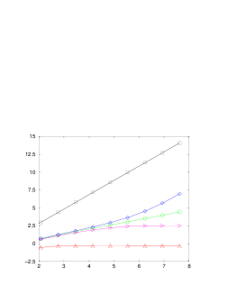
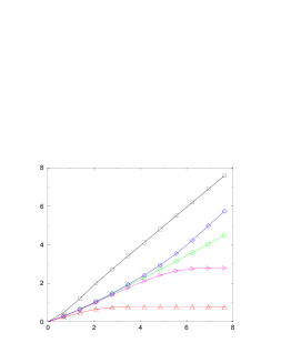
On Fig. 1, we show in log-log scale the RG flows of the typical renormalized transverse field hLt​y​psuperscriptsubscriptβ„ŽπΏπ‘‘π‘¦π‘h_{L}^{typ} of Eq. 65

ln⁑hLt​y​p|ΞΈ<ΞΈcevaluated-atsuperscriptsubscriptβ„ŽπΏπ‘‘π‘¦π‘πœƒsubscriptπœƒπ‘\displaystyle\ln h_{L}^{typ}|_{\theta<\theta_{c}} ∝Lβ†’+βˆžβˆ’L2subscriptproportional-to→𝐿superscript𝐿2\displaystyle\mathop{\propto}_{L\to+\infty}-L^{2}
ln⁑hLt​y​p|ΞΈ=ΞΈcevaluated-atsuperscriptsubscriptβ„ŽπΏπ‘‘π‘¦π‘πœƒsubscriptπœƒπ‘\displaystyle\ln h_{L}^{typ}|_{\theta=\theta_{c}} ∝Lβ†’+βˆžβˆ’LψwithΟˆβ‰ƒ0.65similar-to-or-equalssubscriptproportional-to→𝐿superscriptπΏπœ“withπœ“0.65\displaystyle\mathop{\propto}_{L\to+\infty}-L^{\psi}\ \ {\rm with}\ \ \psi\simeq 0.65
ln⁑hLt​y​p|ΞΈ>ΞΈcevaluated-atsuperscriptsubscriptβ„ŽπΏπ‘‘π‘¦π‘πœƒsubscriptπœƒπ‘\displaystyle\ln h_{L}^{typ}|_{\theta>\theta_{c}} ∝Lβ†’+∞C​s​tsubscriptproportional-to→𝐿𝐢𝑠𝑑\displaystyle\mathop{\propto}_{L\to+\infty}Cst (67)

and of the width Ξ”ln⁑hLsubscriptΞ”subscriptβ„ŽπΏ\Delta_{\ln h_{L}} of Eq. 66

Ξ”ln⁑hL|ΞΈ<ΞΈcevaluated-atsubscriptΞ”subscriptβ„ŽπΏπœƒsubscriptπœƒπ‘\displaystyle\Delta_{\ln h_{L}}|_{\theta<\theta_{c}} ∝Lβ†’+∞Lsubscriptproportional-to→𝐿𝐿\displaystyle\mathop{\propto}_{L\to+\infty}L
Ξ”ln⁑hL|ΞΈ=ΞΈcevaluated-atsubscriptΞ”subscriptβ„ŽπΏπœƒsubscriptπœƒπ‘\displaystyle\Delta_{\ln h_{L}}|_{\theta=\theta_{c}} ∝Lβ†’+∞LψwithΟˆβ‰ƒ0.65similar-to-or-equalssubscriptproportional-to→𝐿superscriptπΏπœ“withπœ“0.65\displaystyle\mathop{\propto}_{L\to+\infty}L^{\psi}\ \ {\rm with}\ \ \psi\simeq 0.65
Ξ”ln⁑hL|ΞΈ>ΞΈcevaluated-atsubscriptΞ”subscriptβ„ŽπΏπœƒsubscriptπœƒπ‘\displaystyle\Delta_{\ln h_{L}}|_{\theta>\theta_{c}} ∝Lβ†’+∞C​s​tsubscriptproportional-to→𝐿𝐢𝑠𝑑\displaystyle\mathop{\propto}_{L\to+\infty}Cst (68)
Refer to caption
Refer to caption
Figure 1: RG flow of the logarithm of the transverse fields in log-log scale
(a) Ya=ln⁑(βˆ’ln⁑hLt​y​p)≑ln⁑(βˆ’ln⁑hLΒ―)subscriptπ‘Œπ‘Žsuperscriptsubscriptβ„ŽπΏπ‘‘π‘¦π‘Β―subscriptβ„ŽπΏY_{a}=\ln(-\ln h_{L}^{typ})\equiv\ln(-\overline{\ln h_{L}}) as a function of X=ln⁑L𝑋𝐿X=\ln L :
(i) Ordered phase ΞΈ<ΞΈcπœƒsubscriptπœƒπ‘\theta<\theta_{c} : the asymptotic slope is d=2𝑑2d=2, as shown here for ΞΈ=0.5πœƒ0.5\theta=0.5 (squares) and ΞΈ=1.245πœƒ1.245\theta=1.245 (diamond)
(ii) Disordered phase ΞΈ>ΞΈcπœƒsubscriptπœƒπ‘\theta>\theta_{c} : the asymptotic slope is 00, as shown here for ΞΈ=1.5πœƒ1.5\theta=1.5 (triangles up) and ΞΈ=1.27πœƒ1.27\theta=1.27 (triangles right)
(iii) Critical point ΞΈc=1.256subscriptπœƒπ‘1.256\theta_{c}=1.256 (circles) : the asymptotic slope is Οˆβ‰ƒ0.65similar-to-or-equalsπœ“0.65\psi\simeq 0.65.
(b) Yb=ln⁑(Ξ”ln⁑hL)≑ln⁑((ln⁑hL)2Β―βˆ’(ln⁑hLΒ―)2)subscriptπ‘Œπ‘subscriptΞ”subscriptβ„ŽπΏΒ―superscriptsubscriptβ„ŽπΏ2superscriptΒ―subscriptβ„ŽπΏ2Y_{b}=\ln(\Delta_{\ln h_{L}})\equiv\ln(\sqrt{\overline{(\ln h_{L})^{2}}-(\overline{\ln h_{L}})^{2}}) as a function of X=ln⁑L𝑋𝐿X=\ln L :
(i) Ordered phase ΞΈ<ΞΈcπœƒsubscriptπœƒπ‘\theta<\theta_{c} : the asymptotic slope is 111, as shown here for ΞΈ=0.5πœƒ0.5\theta=0.5 (squares) and ΞΈ=1.245πœƒ1.245\theta=1.245 (diamond)
(ii) Disordered phase ΞΈ>ΞΈcπœƒsubscriptπœƒπ‘\theta>\theta_{c} : the asymptotic slope is 00, as shown here for ΞΈ=1.5πœƒ1.5\theta=1.5 (triangles up) and ΞΈ=1.27πœƒ1.27\theta=1.27 (triangles right)
(iii) Critical point ΞΈc=1.256subscriptπœƒπ‘1.256\theta_{c}=1.256 (circles) : the asymptotic slope is Οˆβ‰ƒ0.65similar-to-or-equalsπœ“0.65\psi\simeq 0.65.

At the critical point ΞΈcsubscriptπœƒπ‘\theta_{c}, the RG flows of the typical value and of the width display the same activated scaling of an Infinite Disorder Fixed Point

ln⁑hL|ΞΈ=ΞΈcevaluated-atsubscriptβ„ŽπΏπœƒsubscriptπœƒπ‘\displaystyle\ln h_{L}|_{\theta=\theta_{c}} =βˆ’LΟˆβ€‹vcabsentsuperscriptπΏπœ“subscript𝑣𝑐\displaystyle=-L^{\psi}v_{c} (69)

where vcsubscript𝑣𝑐v_{c} is some O​(1)𝑂1O(1) random variable. The values obtained here for the location of the critical point ΞΈc≃1.256similar-to-or-equalssubscriptπœƒπ‘1.256\theta_{c}\simeq 1.256 and the activated exponent Οˆβ‰ƒ0.65similar-to-or-equalsπœ“0.65\psi\simeq 0.65 turn out to be different from the estimations ΞΈcS​D≃1.678similar-to-or-equalssuperscriptsubscriptπœƒπ‘π‘†π·1.678\theta_{c}^{SD}\simeq 1.678 and ψS​D≃0.48similar-to-or-equalssuperscriptπœ“π‘†π·0.48\psi^{SD}\simeq 0.48 obtained via the Strong Disorder Renormalization (see [20, 23] and references therein) : the origin of these differences is not clear to us.

In the ordered phase, the logarithm of the typical renormalized transverse field grows extensively with respect to the volume Ldsuperscript𝐿𝑑L^{d} (with d=2𝑑2d=2 here)

ln⁑hLt​y​pβ€‹βˆLβ†’βˆžβˆ’(LΞΎh)dsuperscriptsubscriptβ„ŽπΏπ‘‘π‘¦π‘subscriptproportional-to→𝐿superscript𝐿subscriptπœ‰β„Žπ‘‘\displaystyle\ln h_{L}^{typ}\mathop{\propto}_{L\to\infty}-\left(\frac{L}{\xi_{h}}\right)^{d} (70)

where the length scale ΞΎhsubscriptπœ‰β„Ž\xi_{h} represents the characteristic size of finite disordered clusters within this ordered phase. From our numerical data concerning the ordered phase, the asymptotic behavior of Eq. 70 allows to measure ΞΎhsubscriptπœ‰β„Ž\xi_{h} and its divergence near criticality

ΞΎhβ€‹βˆΞΈβ†’ΞΈc(ΞΈcβˆ’ΞΈ)βˆ’Ξ½hwithΞ½h≃0.84similar-to-or-equalssubscriptπœ‰β„Žsubscriptproportional-toβ†’πœƒsubscriptπœƒπ‘superscriptsubscriptπœƒπ‘πœƒsubscriptπœˆβ„Žwithsubscriptπœˆβ„Ž0.84\displaystyle\xi_{h}\mathop{\propto}_{\theta\to\theta_{c}}(\theta_{c}-\theta)^{-\nu_{h}}\ \ \ {\rm with}\ \ \ \nu_{h}\simeq 0.84 (71)

In the disordered phase, the asymptotic typical value h∞t​y​psuperscriptsubscriptβ„Žπ‘‘π‘¦π‘h_{\infty}^{typ} diverges with an essential singularity as a function of the control parameter

ln⁑h∞t​y​p≑ln⁑hβˆžΒ―βˆβˆ’(ΞΈβˆ’ΞΈc)βˆ’ΞΊwithκ≃0.82formulae-sequencesuperscriptsubscriptβ„Žπ‘‘π‘¦π‘Β―subscriptβ„Žproportional-tosuperscriptπœƒsubscriptπœƒπ‘πœ…similar-to-or-equalswithπœ…0.82\displaystyle\ln h_{\infty}^{typ}\equiv\overline{\ln h_{\infty}}\propto-(\theta-\theta_{c})^{-\kappa}\ \ \ {\rm with}\ \ \ \kappa\simeq 0.82 (72)

In the critical region, the finite-size scaling form is governed by some finite-size scaling correlation length exponent Ξ½F​SsubscriptπœˆπΉπ‘†\nu_{FS}

ln⁑hLt​y​p≑ln⁑hLΒ―=βˆ’LΟˆβ€‹Fh​(L1Ξ½F​S​(ΞΈβˆ’ΞΈc))superscriptsubscriptβ„ŽπΏπ‘‘π‘¦π‘Β―subscriptβ„ŽπΏsuperscriptπΏπœ“subscriptπΉβ„Žsuperscript𝐿1subscriptπœˆπΉπ‘†πœƒsubscriptπœƒπ‘\displaystyle\ln h_{L}^{typ}\equiv\overline{\ln h_{L}}=-L^{\psi}F_{h}\left(L^{\frac{1}{\nu_{FS}}}(\theta-\theta_{c})\right) (73)

The matching with the behavior in the ordered phase (Eqs 70 and 71) and in the disordered phase (Eq. 72) yields the relations

Ξ½h=(1βˆ’Οˆd)​νF​Ssubscriptπœˆβ„Ž1πœ“π‘‘subscriptπœˆπΉπ‘†\displaystyle\nu_{h}=\left(1-\frac{\psi}{d}\right)\nu_{FS} (74)

and

ΞΊ=Οˆβ€‹Ξ½F​Sπœ…πœ“subscriptπœˆπΉπ‘†\displaystyle\kappa=\psi\nu_{FS} (75)

The previous numerical measures of Οˆπœ“\psi, Ξ½hsubscriptπœˆβ„Ž\nu_{h} and ΞΊπœ…\kappa yield the estimate

Ξ½F​S≃1.25similar-to-or-equalssubscriptπœˆπΉπ‘†1.25\displaystyle\nu_{FS}\simeq 1.25 (76)

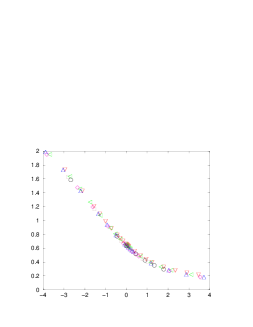
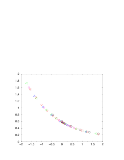
As shown on Fig. 2, this value of Ξ½F​SsubscriptπœˆπΉπ‘†\nu_{FS} gives satisfactory finite-size scaling plots of the numerical data of Fig. 1.
Refer to caption
Refer to caption
Figure 2: Finite-size scaling plots of the numerical data of Fig. 1 corresponding to the sizes 26≀L≀211superscript26𝐿superscript2112^{6}\leq L\leq 2^{11} with the values ΞΈc=1.256subscriptπœƒπ‘1.256\theta_{c}=1.256 for the critical point and Ξ½F​S=1.25subscriptπœˆπΉπ‘†1.25\nu_{FS}=1.25 for the finite-size correlation length exponent :
(a) Ya=(βˆ’ln⁑hLt​y​pLψ)subscriptπ‘Œπ‘Žsuperscriptsubscriptβ„ŽπΏπ‘‘π‘¦π‘superscriptπΏπœ“Y_{a}=\left(-\frac{\ln h_{L}^{typ}}{L^{\psi}}\right) as a function of X=(ΞΈβˆ’ΞΈc)​L1Ξ½F​Sπ‘‹πœƒsubscriptπœƒπ‘superscript𝐿1subscriptπœˆπΉπ‘†X=(\theta-\theta_{c})L^{\frac{1}{\nu_{FS}}}.
(b) Yb=(Ξ”ln⁑hLLψ)subscriptπ‘Œπ‘subscriptΞ”subscriptβ„ŽπΏsuperscriptπΏπœ“Y_{b}=\left(\frac{\Delta_{\ln h_{L}}}{L^{\psi}}\right) as a function of X=(ΞΈβˆ’ΞΈc)​L1Ξ½F​Sπ‘‹πœƒsubscriptπœƒπ‘superscript𝐿1subscriptπœˆπΉπ‘†X=(\theta-\theta_{c})L^{\frac{1}{\nu_{FS}}}.

This value for Ξ½F​SsubscriptπœˆπΉπ‘†\nu_{FS} (Eq. 76) agrees with the estimations obtained via the Strong Disorder Renormalization (see [20, 23] and references therein), and with the asymmetric block renormalization of Ref [26].

VI.3 RG flow of the renormalized couplings
Refer to caption
Refer to caption
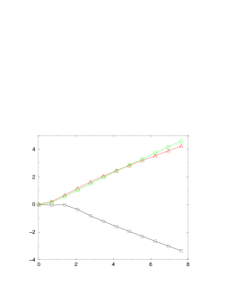
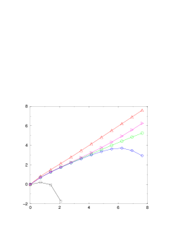
Figure 3: RG flow of the logarithm of the couplings in log-log scale
(a) Ya=ln⁑(βˆ’ln⁑JLt​y​p)≑ln⁑(βˆ’ln⁑JLΒ―)subscriptπ‘Œπ‘Žsuperscriptsubscript𝐽𝐿𝑑𝑦𝑝¯subscript𝐽𝐿Y_{a}=\ln(-\ln J_{L}^{typ})\equiv\ln(-\overline{\ln J_{L}}) as a function of X=ln⁑L𝑋𝐿X=\ln L :
(i) Ordered phase ΞΈ<ΞΈcπœƒsubscriptπœƒπ‘\theta<\theta_{c} : the flow is non-monotonic, as shown here for ΞΈ=0.5πœƒ0.5\theta=0.5 (squares) and ΞΈ=1.245πœƒ1.245\theta=1.245 (diamond) : the asymptotic behavior (not visible on this plot appropriate to the critical region) corresponds to the classical random ferromagnet growth JLt​y​p∝Ldβˆ’1=Lproportional-tosuperscriptsubscript𝐽𝐿𝑑𝑦𝑝superscript𝐿𝑑1𝐿J_{L}^{typ}\propto L^{d-1}=L
(ii) Disordered phase ΞΈ>ΞΈcπœƒsubscriptπœƒπ‘\theta>\theta_{c} : the asymptotic slope is 111, as shown here for ΞΈ=1.5πœƒ1.5\theta=1.5 (triangles up) and ΞΈ=1.27πœƒ1.27\theta=1.27 (triangles right)
(iii) Critical point ΞΈc=1.256subscriptπœƒπ‘1.256\theta_{c}=1.256 (circles) : the asymptotic slope is Οˆβ‰ƒ0.65similar-to-or-equalsπœ“0.65\psi\simeq 0.65.
(b) Yb=ln⁑Δln⁑JL≑ln⁑((ln⁑JL)2Β―βˆ’(ln⁑JLΒ―)2)subscriptπ‘Œπ‘subscriptΞ”subscript𝐽𝐿¯superscriptsubscript𝐽𝐿2superscriptΒ―subscript𝐽𝐿2Y_{b}=\ln\Delta_{\ln J_{L}}\equiv\ln(\sqrt{\overline{(\ln J_{L})^{2}}-(\overline{\ln J_{L}})^{2}}) as a function of X=ln⁑L𝑋𝐿X=\ln L :
(i) Ordered phase ΞΈ<ΞΈcπœƒsubscriptπœƒπ‘\theta<\theta_{c} : the asymptotic slope is (βˆ’1/2)12(-1/2), as shown here for ΞΈ=0.5πœƒ0.5\theta=0.5 (squares)
(ii) Disordered phase ΞΈ>ΞΈcπœƒsubscriptπœƒπ‘\theta>\theta_{c} : the asymptotic slope is (+1/2)12(+1/2), as shown here for ΞΈ=1.5πœƒ1.5\theta=1.5 (triangles up)
(iii) Critical point ΞΈc=1.256subscriptπœƒπ‘1.256\theta_{c}=1.256 (circles) : the asymptotic slope is Οˆβ‰ƒ0.65similar-to-or-equalsπœ“0.65\psi\simeq 0.65.

On Fig. 3, we show in log-log scale the RG flows of the typical renormalized coupling JLt​y​psuperscriptsubscript𝐽𝐿𝑑𝑦𝑝J_{L}^{typ} of Eq. 65

ln⁑JLt​y​p|ΞΈ<ΞΈcevaluated-atsuperscriptsubscriptπ½πΏπ‘‘π‘¦π‘πœƒsubscriptπœƒπ‘\displaystyle\ln J_{L}^{typ}|_{\theta<\theta_{c}} ∝Lβ†’+∞ln⁑Lsubscriptproportional-to→𝐿𝐿\displaystyle\mathop{\propto}_{L\to+\infty}\ln L
ln⁑JLt​y​p|ΞΈ=ΞΈcevaluated-atsuperscriptsubscriptπ½πΏπ‘‘π‘¦π‘πœƒsubscriptπœƒπ‘\displaystyle\ln J_{L}^{typ}|_{\theta=\theta_{c}} ∝Lβ†’+βˆžβˆ’LψwithΟˆβ‰ƒ0.65similar-to-or-equalssubscriptproportional-to→𝐿superscriptπΏπœ“withπœ“0.65\displaystyle\mathop{\propto}_{L\to+\infty}-L^{\psi}\ \ {\rm with}\ \ \psi\simeq 0.65
ln⁑JLt​y​p|ΞΈ>ΞΈcevaluated-atsuperscriptsubscriptπ½πΏπ‘‘π‘¦π‘πœƒsubscriptπœƒπ‘\displaystyle\ln J_{L}^{typ}|_{\theta>\theta_{c}} ∝Lβ†’+βˆžβˆ’Lsubscriptproportional-to→𝐿𝐿\displaystyle\mathop{\propto}_{L\to+\infty}-L (77)

and of the width Ξ”ln⁑JLsubscriptΞ”subscript𝐽𝐿\Delta_{\ln J_{L}} of Eq. 66

Ξ”ln⁑JL|ΞΈ<ΞΈcevaluated-atsubscriptΞ”subscriptπ½πΏπœƒsubscriptπœƒπ‘\displaystyle\Delta_{\ln J_{L}}|_{\theta<\theta_{c}} ∝Lβ†’+∞Lβˆ’12subscriptproportional-to→𝐿superscript𝐿12\displaystyle\mathop{\propto}_{L\to+\infty}L^{-\frac{1}{2}}
Ξ”ln⁑JL|ΞΈ=ΞΈcevaluated-atsubscriptΞ”subscriptπ½πΏπœƒsubscriptπœƒπ‘\displaystyle\Delta_{\ln J_{L}}|_{\theta=\theta_{c}} ∝Lβ†’+∞LψwithΟˆβ‰ƒ0.65similar-to-or-equalssubscriptproportional-to→𝐿superscriptπΏπœ“withπœ“0.65\displaystyle\mathop{\propto}_{L\to+\infty}L^{\psi}\ \ {\rm with}\ \ \psi\simeq 0.65
Ξ”ln⁑JL|ΞΈ>ΞΈcevaluated-atsubscriptΞ”subscriptπ½πΏπœƒsubscriptπœƒπ‘\displaystyle\Delta_{\ln J_{L}}|_{\theta>\theta_{c}} ∝Lβ†’+∞L12subscriptproportional-to→𝐿superscript𝐿12\displaystyle\mathop{\propto}_{L\to+\infty}L^{\frac{1}{2}} (78)

At the critical point ΞΈc≃1.256similar-to-or-equalssubscriptπœƒπ‘1.256\theta_{c}\simeq 1.256, the RG flows of the typical value and of the width display the same activated scaling of Infinite Disorder Fixed Point as in Eq. 69

ln⁑JLsubscript𝐽𝐿\displaystyle\ln J_{L} =βˆ’LΟˆβ€‹ucabsentsuperscriptπΏπœ“subscript𝑒𝑐\displaystyle=-L^{\psi}u_{c} (79)

where ucsubscript𝑒𝑐u_{c} is some O​(1)𝑂1O(1) random variable.

In the disordered phase, the typical renormalized coupling JLt​y​psuperscriptsubscript𝐽𝐿𝑑𝑦𝑝J_{L}^{typ} decays exponentially with the size L𝐿L

ln⁑JLt​y​p≑ln⁑JLΒ―β€‹βˆLβ†’+βˆžβˆ’LΞΎt​y​psuperscriptsubscript𝐽𝐿𝑑𝑦𝑝¯subscript𝐽𝐿subscriptproportional-to→𝐿𝐿subscriptπœ‰π‘‘π‘¦π‘\displaystyle\ln J_{L}^{typ}\equiv\overline{\ln J_{L}}\mathop{\propto}_{L\to+\infty}-\frac{L}{\xi_{typ}} (80)

where ΞΎt​y​psubscriptπœ‰π‘‘π‘¦π‘\xi_{typ} represents the typical correlation length. From our numerical data concerning the disordered phase, the asymptotic behavior of Eq. 80 allows to measure ΞΎt​y​psubscriptπœ‰π‘‘π‘¦π‘\xi_{typ} and its divergence near criticality

ΞΎt​y​pβˆΞΈβ†’ΞΈc(ΞΈcβˆ’ΞΈ)βˆ’Ξ½t​y​pwithΞ½t​y​p≃0.44formulae-sequencesubscriptproportional-toβ†’πœƒsubscriptπœƒπ‘subscriptπœ‰π‘‘π‘¦π‘superscriptsubscriptπœƒπ‘πœƒsubscriptπœˆπ‘‘π‘¦π‘withsimilar-to-or-equalssubscriptπœˆπ‘‘π‘¦π‘0.44\displaystyle\xi_{typ}\propto_{\theta\to\theta_{c}}(\theta_{c}-\theta)^{-\nu_{typ}}\ \ \ {\rm with}\ \ \ \nu_{typ}\simeq 0.44 (81)

The compatibility with the finite-size scaling form analogous to Eq. 73

ln⁑JLt​y​p≑ln⁑JLΒ―=βˆ’LΟˆβ€‹FJ​(L1Ξ½F​S​(ΞΈβˆ’ΞΈc))superscriptsubscript𝐽𝐿𝑑𝑦𝑝¯subscript𝐽𝐿superscriptπΏπœ“subscript𝐹𝐽superscript𝐿1subscriptπœˆπΉπ‘†πœƒsubscriptπœƒπ‘\displaystyle\ln J_{L}^{typ}\equiv\overline{\ln J_{L}}=-L^{\psi}F_{J}\left(L^{\frac{1}{\nu_{FS}}}(\theta-\theta_{c})\right) (82)

implies the relation

Ξ½t​y​p=(1βˆ’Οˆ)​νF​Ssubscriptπœˆπ‘‘π‘¦π‘1πœ“subscriptπœˆπΉπ‘†\displaystyle\nu_{typ}=(1-\psi)\nu_{FS} (83)

It is satisfied by the previously quoted estimates of Ξ½t​y​psubscriptπœˆπ‘‘π‘¦π‘\nu_{typ}, Ξ½F​SsubscriptπœˆπΉπ‘†\nu_{FS} and Οˆπœ“\psi.

VII Application to the two-dimensional spin-glass quantum Ising model

To study the two-dimensional spin-glass quantum Ising model, we have replaced the probability distribution of Eq. 61 concerning the random ferromagnetic case by the flat distribution of zero-mean

PS​G​(J)=12​θ​(βˆ’1≀J≀1)subscript𝑃𝑆𝐺𝐽12πœƒ1𝐽1\displaystyle P_{SG}(J)=\frac{1}{2}\theta(-1\leq J\leq 1) (84)

We have then repeated exactly the same numerical analysis as in the previous section VI : the critical point is now found at ΞΈc≃1.088similar-to-or-equalssubscriptπœƒπ‘1.088\theta_{c}\simeq 1.088, and the critical exponents Οˆβ‰ƒ0.65similar-to-or-equalsπœ“0.65\psi\simeq 0.65, Ξ½h≃0.84similar-to-or-equalssubscriptπœˆβ„Ž0.84\nu_{h}\simeq 0.84, Ξ½t​y​p≃0.44similar-to-or-equalssubscriptπœˆπ‘‘π‘¦π‘0.44\nu_{typ}\simeq 0.44, Ξ½F​S≃1.25similar-to-or-equalssubscriptπœˆπΉπ‘†1.25\nu_{FS}\simeq 1.25 are the same as for the random ferromagnet presented in the previous section, as expected for Infinite Disorder Fixed Points [13, 14], and as found within the Miyasaki-Nishimori asymmetric scheme [26].

VIII Conclusion

In this paper, we have proposed a simple generalization in d>1𝑑1d>1 of the self-dual block renormalization procedure of Fernandez-Pacheco [2], that we have tested for pure and random quantum Ising models, with the following conclusions.

For the pure models, where the Fernandez-Pacheco procedure is known to reproduce the exact correlation length exponent ν​(d=1)=1πœˆπ‘‘11\nu(d=1)=1 [2], we have obtained ν​(d=2)≃0.625similar-to-or-equalsπœˆπ‘‘20.625\nu(d=2)\simeq 0.625 (to be compared with the 3D classical Ising model exponent ν≃0.63similar-to-or-equals𝜈0.63\nu\simeq 0.63) and ν​(d=3)≃0.5018similar-to-or-equalsπœˆπ‘‘30.5018\nu(d=3)\simeq 0.5018 (to be compared with the 4D classical Ising model mean-field exponent Ξ½=1/2𝜈12\nu=1/2).

For the random models, where the Fernandez-Pacheco procedure is known to reproduce exactly the location of the critical point and the critical exponents ψ(=1)=1/2annotatedπœ“absent112\psi(=1)=1/2, Ξ½t​y​p=1subscriptπœˆπ‘‘π‘¦π‘1\nu_{typ}=1 and Ξ½F​S=2subscriptπœˆπΉπ‘†2\nu_{FS}=2 of the Infinite Disorder Fixed Point [26], we have applied numerically the renormalization rules to two-dimensional samples of linear size L=4096𝐿4096L=4096, with either random ferromagnetic disorder or spin-glass disorder, both types of disorder leading to the same Infinite Disorder Fixed Point : the finite-size correlation exponent Ξ½F​S≃1.25similar-to-or-equalssubscriptπœˆπΉπ‘†1.25\nu_{FS}\simeq 1.25 coincides with Strong Disorder Renormalization result (see [20, 23] and references therein), and with the asymmetric block renormalization of Ref [26], but the activated exponent Οˆβ‰ƒ0.65similar-to-or-equalsπœ“0.65\psi\simeq 0.65 turns out to be somewhat higher than Strong Disorder Renormalization estimate Οˆβ‰ƒ0.48similar-to-or-equalsπœ“0.48\psi\simeq 0.48 (see [20, 23] and references therein). The origin of this difference remains to be clarified. We have also analyzed the RG flows in the disordered and ordered phases, in order to extract the typical correlation length exponent Ξ½t​y​p≃0.44similar-to-or-equalssubscriptπœˆπ‘‘π‘¦π‘0.44\nu_{typ}\simeq 0.44 and the analog Ξ½h≃0.84similar-to-or-equalssubscriptπœˆβ„Ž0.84\nu_{h}\simeq 0.84, and tested the finite-size scaling.

In summary, the generalization in d>1𝑑1d>1 of the self-dual block renormalization procedure of Fernandez-Pacheco [2] is able to reproduce both the conventional scaling of pure critical points and the activated scaling of Infinite Disorder Fixed Points. It would be thus interesting to develop such methods in models governed by Strong (not Infinite) Disorder Fixed Points like the Quantum Ising model with long-ranged interactions [37] or the superfluid-insulator transition [38], as well as in models where the transition at weak disorder could be in another universality class [38, 39].

Appendix A Renormalization Rules in d=3𝑑3d=3

The initial quantum Hamiltonian on the cubic lattice reads

H=βˆ’βˆ‘(i,j,k)h​(i,j,k)​σ(i,j,k)xβˆ’βˆ‘(i,j,k)Οƒ(i,j,k)z​[Jx→​(i,j,k)​σ(i+1,j,k)z+Jy→​(i,j,k)​σ(i,j+1,k)z+Jz→​(i,j,k)​σ(i,j,k+1)z]𝐻subscriptπ‘–π‘—π‘˜β„Žπ‘–π‘—π‘˜superscriptsubscriptπœŽπ‘–π‘—π‘˜π‘₯subscriptπ‘–π‘—π‘˜superscriptsubscriptπœŽπ‘–π‘—π‘˜π‘§delimited-[]subscript𝐽→π‘₯π‘–π‘—π‘˜superscriptsubscriptπœŽπ‘–1π‘—π‘˜π‘§subscriptπ½β†’π‘¦π‘–π‘—π‘˜superscriptsubscriptπœŽπ‘–π‘—1π‘˜π‘§subscriptπ½β†’π‘§π‘–π‘—π‘˜superscriptsubscriptπœŽπ‘–π‘—π‘˜1𝑧\displaystyle H=-\sum_{(i,j,k)}h(i,j,k)\sigma_{(i,j,k)}^{x}-\sum_{(i,j,k)}\sigma_{(i,j,k)}^{z}\left[J_{\vec{x}}(i,j,k)\sigma_{(i+1,j,k)}^{z}+J_{\vec{y}}(i,j,k)\sigma_{(i,j+1,k)}^{z}+J_{\vec{z}}(i,j,k)\sigma_{(i,j,k+1)}^{z}\right] (85)

We wish to define a block renormalization rule, where each block of 23=8superscript2382^{3}=8 spins (Οƒ2​i,2​j,2​ksubscript𝜎2𝑖2𝑗2π‘˜\sigma_{2i,2j,2k}; Οƒ2​iβˆ’1,2​j,2​ksubscript𝜎2𝑖12𝑗2π‘˜\sigma_{2i-1,2j,2k}; Οƒ2​i,2​jβˆ’1,2​ksubscript𝜎2𝑖2𝑗12π‘˜\sigma_{2i,2j-1,2k}; Οƒ2​i,2​j,2​kβˆ’1subscript𝜎2𝑖2𝑗2π‘˜1\sigma_{2i,2j,2k-1}; Οƒ2​iβˆ’1,2​jβˆ’1,2​ksubscript𝜎2𝑖12𝑗12π‘˜\sigma_{2i-1,2j-1,2k}; Οƒ2​iβˆ’1,2​j,2​kβˆ’1subscript𝜎2𝑖12𝑗2π‘˜1\sigma_{2i-1,2j,2k-1}; Οƒ2​i,2​jβˆ’1,2​kβˆ’1subscript𝜎2𝑖2𝑗12π‘˜1\sigma_{2i,2j-1,2k-1}; Οƒ2​iβˆ’1,2​jβˆ’1,2​kβˆ’1subscript𝜎2𝑖12𝑗12π‘˜1\sigma_{2i-1,2j-1,2k-1}) will be replaced by a single renormalized spin (Οƒ2​i,2​j,2​kR​R​R)superscriptsubscript𝜎2𝑖2𝑗2π‘˜π‘…π‘…π‘…(\sigma_{2i,2j,2k}^{RRR}), after three elementary renormalization steps.

It is thus convenient to start by rewriting Eq. 85 as

H=βˆ‘(i,j,k)Hi,j,k𝐻subscriptπ‘–π‘—π‘˜subscriptπ»π‘–π‘—π‘˜\displaystyle H=\sum_{(i,j,k)}H_{i,j,k}
Hi,j,k=βˆ’h​(2​i,2​j,2​k)​σ(2​i,2​j,2​k)xβˆ’h​(2​iβˆ’1,2​jβˆ’1,2​kβˆ’1)​σ(2​iβˆ’1,2​jβˆ’1,2​kβˆ’1)xsubscriptπ»π‘–π‘—π‘˜β„Ž2𝑖2𝑗2π‘˜superscriptsubscript𝜎2𝑖2𝑗2π‘˜π‘₯β„Ž2𝑖12𝑗12π‘˜1superscriptsubscript𝜎2𝑖12𝑗12π‘˜1π‘₯\displaystyle H_{i,j,k}=-h(2i,2j,2k)\sigma_{(2i,2j,2k)}^{x}-h(2i-1,2j-1,2k-1)\sigma_{(2i-1,2j-1,2k-1)}^{x}
βˆ’h​(2​iβˆ’1,2​j,2​k)​σ(2​iβˆ’1,2​j,2​k)xβˆ’h​(2​i,2​jβˆ’1,2​k)​σ(2​i,2​jβˆ’1,2​k)xβˆ’h​(2​i,2​j,2​kβˆ’1)​σ(2​i,2​j,2​kβˆ’1)xβ„Ž2𝑖12𝑗2π‘˜superscriptsubscript𝜎2𝑖12𝑗2π‘˜π‘₯β„Ž2𝑖2𝑗12π‘˜superscriptsubscript𝜎2𝑖2𝑗12π‘˜π‘₯β„Ž2𝑖2𝑗2π‘˜1superscriptsubscript𝜎2𝑖2𝑗2π‘˜1π‘₯\displaystyle-h(2i-1,2j,2k)\sigma_{(2i-1,2j,2k)}^{x}-h(2i,2j-1,2k)\sigma_{(2i,2j-1,2k)}^{x}-h(2i,2j,2k-1)\sigma_{(2i,2j,2k-1)}^{x}
βˆ’h​(2​iβˆ’1,2​jβˆ’1,2​k)​σ(2​iβˆ’1,2​jβˆ’1,2​k)xβˆ’h​(2​i,2​jβˆ’1,2​kβˆ’1)​σ(2​i,2​jβˆ’1,2​kβˆ’1)xβˆ’h​(2​iβˆ’1,2​j,2​kβˆ’1)​σ(2​iβˆ’1,2​j,2​kβˆ’1)xβ„Ž2𝑖12𝑗12π‘˜superscriptsubscript𝜎2𝑖12𝑗12π‘˜π‘₯β„Ž2𝑖2𝑗12π‘˜1superscriptsubscript𝜎2𝑖2𝑗12π‘˜1π‘₯β„Ž2𝑖12𝑗2π‘˜1superscriptsubscript𝜎2𝑖12𝑗2π‘˜1π‘₯\displaystyle-h(2i-1,2j-1,2k)\sigma_{(2i-1,2j-1,2k)}^{x}-h(2i,2j-1,2k-1)\sigma_{(2i,2j-1,2k-1)}^{x}-h(2i-1,2j,2k-1)\sigma_{(2i-1,2j,2k-1)}^{x}
βˆ’Οƒ(2​iβˆ’1,2​j,2​k)z[Jxβ†’(2iβˆ’1,2j,2k)Οƒ(2​i,2​j,2​k)z+Jyβ†’(2iβˆ’1,2j,2k)Οƒ(2​iβˆ’1,2​j+1,2​k)z+Jzβ†’(2iβˆ’1,2j,2k)Οƒ(2​iβˆ’1,2​j,2​k+1)z\displaystyle-\sigma_{(2i-1,2j,2k)}^{z}[J_{\vec{x}}(2i-1,2j,2k)\sigma_{(2i,2j,2k)}^{z}+J_{\vec{y}}(2i-1,2j,2k)\sigma_{(2i-1,2j+1,2k)}^{z}+J_{\vec{z}}(2i-1,2j,2k)\sigma_{(2i-1,2j,2k+1)}^{z}
+Jxβ†’(2iβˆ’2,2j,2k)Οƒ(2​iβˆ’2,2​j,2​k)z+Jyβ†’(2iβˆ’1,2jβˆ’1,2k)Οƒ(2​iβˆ’1,2​jβˆ’1,2​k)z+Jzβ†’(2iβˆ’1,2j,2kβˆ’1)Οƒ(2​iβˆ’1,2​j,2​kβˆ’1)z]\displaystyle+J_{\vec{x}}(2i-2,2j,2k)\sigma_{(2i-2,2j,2k)}^{z}+J_{\vec{y}}(2i-1,2j-1,2k)\sigma_{(2i-1,2j-1,2k)}^{z}+J_{\vec{z}}(2i-1,2j,2k-1)\sigma_{(2i-1,2j,2k-1)}^{z}]
βˆ’Οƒ(2​i,2​jβˆ’1,2​k)z[Jyβ†’(2i,2jβˆ’1,2k)Οƒ(2​i,2​j,2​k)z+Jxβ†’(2i,2jβˆ’1,2k)Οƒ(2​i+1,2​jβˆ’1,2​k)z+Jzβ†’(2i,2jβˆ’1,2k)Οƒ(2​i,2​jβˆ’1,2​k+1)z\displaystyle-\sigma_{(2i,2j-1,2k)}^{z}[J_{\vec{y}}(2i,2j-1,2k)\sigma_{(2i,2j,2k)}^{z}+J_{\vec{x}}(2i,2j-1,2k)\sigma_{(2i+1,2j-1,2k)}^{z}+J_{\vec{z}}(2i,2j-1,2k)\sigma_{(2i,2j-1,2k+1)}^{z}
+Jyβ†’(2i,2jβˆ’2,2k)Οƒ(2​i,2​jβˆ’2,2​k)z+Jxβ†’(2iβˆ’1,2jβˆ’1,2k)Οƒ(2​iβˆ’1,2​jβˆ’1,2​k)z+Jzβ†’(2i,2jβˆ’1,2kβˆ’1)Οƒ(2​i,2​jβˆ’1,2​kβˆ’1)z]\displaystyle+J_{\vec{y}}(2i,2j-2,2k)\sigma_{(2i,2j-2,2k)}^{z}+J_{\vec{x}}(2i-1,2j-1,2k)\sigma_{(2i-1,2j-1,2k)}^{z}+J_{\vec{z}}(2i,2j-1,2k-1)\sigma_{(2i,2j-1,2k-1)}^{z}]
βˆ’Οƒ(2​i,2​j,2​kβˆ’1)z[Jzβ†’(2i,2j,2kβˆ’1)Οƒ(2​i,2​j,2​k)z+Jxβ†’(2i,2j,2kβˆ’1)Οƒ(2​i+1,2​j,2​kβˆ’1)z+Jyβ†’(2i,2j,2kβˆ’1)Οƒ(2​i,2​j+1,2​kβˆ’1)z\displaystyle-\sigma_{(2i,2j,2k-1)}^{z}[J_{\vec{z}}(2i,2j,2k-1)\sigma_{(2i,2j,2k)}^{z}+J_{\vec{x}}(2i,2j,2k-1)\sigma_{(2i+1,2j,2k-1)}^{z}+J_{\vec{y}}(2i,2j,2k-1)\sigma_{(2i,2j+1,2k-1)}^{z}
+Jzβ†’(2i,2j,2kβˆ’2)Οƒ(2​i,2​j,2​kβˆ’2)z+Jxβ†’(2iβˆ’1,2j,2kβˆ’1)Οƒ(2​iβˆ’1,2​j,2​kβˆ’1)z+Jyβ†’(2i,2jβˆ’1,2kβˆ’1)Οƒ(2​i,2​jβˆ’1,2​kβˆ’1)z]\displaystyle+J_{\vec{z}}(2i,2j,2k-2)\sigma_{(2i,2j,2k-2)}^{z}+J_{\vec{x}}(2i-1,2j,2k-1)\sigma_{(2i-1,2j,2k-1)}^{z}+J_{\vec{y}}(2i,2j-1,2k-1)\sigma_{(2i,2j-1,2k-1)}^{z}]
βˆ’Οƒ(2​iβˆ’1,2​jβˆ’1,2​kβˆ’1)z[Jxβ†’(2iβˆ’1,2jβˆ’1,2kβˆ’1)Οƒ(2​iβˆ’1,2​jβˆ’1,2​k)z+Jyβ†’(2iβˆ’1,2jβˆ’1,2kβˆ’1)Οƒ(2​iβˆ’1,2​j,2​kβˆ’1)z\displaystyle-\sigma_{(2i-1,2j-1,2k-1)}^{z}[J_{\vec{x}}(2i-1,2j-1,2k-1)\sigma_{(2i-1,2j-1,2k)}^{z}+J_{\vec{y}}(2i-1,2j-1,2k-1)\sigma_{(2i-1,2j,2k-1)}^{z}
+Jz→​(2​iβˆ’1,2​jβˆ’1,2​kβˆ’1)​σ(2​iβˆ’1,2​jβˆ’1,2​k)z+Jx→​(2​iβˆ’2,2​jβˆ’1,2​kβˆ’1)​σ(2​iβˆ’2,2​jβˆ’1,2​kβˆ’1)zsubscript𝐽→𝑧2𝑖12𝑗12π‘˜1superscriptsubscript𝜎2𝑖12𝑗12π‘˜π‘§subscript𝐽→π‘₯2𝑖22𝑗12π‘˜1superscriptsubscript𝜎2𝑖22𝑗12π‘˜1𝑧\displaystyle+J_{\vec{z}}(2i-1,2j-1,2k-1)\sigma_{(2i-1,2j-1,2k)}^{z}+J_{\vec{x}}(2i-2,2j-1,2k-1)\sigma_{(2i-2,2j-1,2k-1)}^{z}
+Jyβ†’(2iβˆ’1,2jβˆ’2,2kβˆ’1)Οƒ(2​iβˆ’1,2​jβˆ’2,2​kβˆ’1)z+Jzβ†’(2iβˆ’1,2jβˆ’1,2kβˆ’2)Οƒ(2​iβˆ’1,2​jβˆ’1,2​kβˆ’2)z]\displaystyle+J_{\vec{y}}(2i-1,2j-2,2k-1)\sigma_{(2i-1,2j-2,2k-1)}^{z}+J_{\vec{z}}(2i-1,2j-1,2k-2)\sigma_{(2i-1,2j-1,2k-2)}^{z}] (86)

A.1 First renormalization step

In the first renormalization step, we choose the following intra-block Hamiltonian

Hi​n​t​r​a(1)β‰‘βˆ’h​(2​iβˆ’1,2​j,2​k)​σ2​iβˆ’1,2​j,2​kxβˆ’Jx→​(2​iβˆ’1,2​j,2​k)​σ2​iβˆ’1,2​j,2​kz​σ2​i,2​j,2​kzsuperscriptsubscriptπ»π‘–π‘›π‘‘π‘Ÿπ‘Ž1β„Ž2𝑖12𝑗2π‘˜superscriptsubscript𝜎2𝑖12𝑗2π‘˜π‘₯subscript𝐽→π‘₯2𝑖12𝑗2π‘˜superscriptsubscript𝜎2𝑖12𝑗2π‘˜π‘§superscriptsubscript𝜎2𝑖2𝑗2π‘˜π‘§\displaystyle H_{intra}^{(1)}\equiv-h(2i-1,2j,2k)\sigma_{2i-1,2j,2k}^{x}-J_{\vec{x}}(2i-1,2j,2k)\sigma_{2i-1,2j,2k}^{z}\sigma_{2i,2j,2k}^{z}
βˆ’h​(2​i,2​jβˆ’1,2​k)​σ2​i,2​jβˆ’1,2​kxβˆ’Jy→​(2​i,2​jβˆ’1,2​k)​σ2​i,2​jβˆ’1,2​kz​σ2​i,2​j,2​kzβ„Ž2𝑖2𝑗12π‘˜superscriptsubscript𝜎2𝑖2𝑗12π‘˜π‘₯subscript𝐽→𝑦2𝑖2𝑗12π‘˜superscriptsubscript𝜎2𝑖2𝑗12π‘˜π‘§superscriptsubscript𝜎2𝑖2𝑗2π‘˜π‘§\displaystyle-h(2i,2j-1,2k)\sigma_{2i,2j-1,2k}^{x}-J_{\vec{y}}(2i,2j-1,2k)\sigma_{2i,2j-1,2k}^{z}\sigma_{2i,2j,2k}^{z}
βˆ’h​(2​i,2​j,2​kβˆ’1)​σ2​i,2​j,2​kβˆ’1xβˆ’Jz→​(2​i,2​j,2​kβˆ’1)​σ2​i,2​j,2​kβˆ’1z​σ2​i,2​j,2​kzβ„Ž2𝑖2𝑗2π‘˜1superscriptsubscript𝜎2𝑖2𝑗2π‘˜1π‘₯subscript𝐽→𝑧2𝑖2𝑗2π‘˜1superscriptsubscript𝜎2𝑖2𝑗2π‘˜1𝑧superscriptsubscript𝜎2𝑖2𝑗2π‘˜π‘§\displaystyle-h(2i,2j,2k-1)\sigma_{2i,2j,2k-1}^{x}-J_{\vec{z}}(2i,2j,2k-1)\sigma_{2i,2j,2k-1}^{z}\sigma_{2i,2j,2k}^{z} (87)

It has the form the Hamiltonian of Eq. 2 analyzed in section II, so that the four spins ( Οƒ2​i,2​j,2​ksubscript𝜎2𝑖2𝑗2π‘˜\sigma_{2i,2j,2k}; Οƒ2​iβˆ’1,2​j,2​ksubscript𝜎2𝑖12𝑗2π‘˜\sigma_{2i-1,2j,2k} ; Οƒ2​i,2​jβˆ’1,2​ksubscript𝜎2𝑖2𝑗12π‘˜\sigma_{2i,2j-1,2k} ;Οƒ2​i,2​j,2​kβˆ’1subscript𝜎2𝑖2𝑗2π‘˜1\sigma_{2i,2j,2k-1} ) are replaced by a single renormalized spin (Οƒ2​i,2​j,2​kR)superscriptsubscript𝜎2𝑖2𝑗2π‘˜π‘…(\sigma_{2i,2j,2k}^{R}), whereas the four other spins Οƒ2​iβˆ’1,2​jβˆ’1,2​k;Οƒ2​iβˆ’1,2​j,2​kβˆ’1;Οƒ2​i,2​jβˆ’1,2​kβˆ’1;Οƒ2​iβˆ’1,2​jβˆ’1,2​kβˆ’1subscript𝜎2𝑖12𝑗12π‘˜subscript𝜎2𝑖12𝑗2π‘˜1subscript𝜎2𝑖2𝑗12π‘˜1subscript𝜎2𝑖12𝑗12π‘˜1\sigma_{2i-1,2j-1,2k};\sigma_{2i-1,2j,2k-1};\sigma_{2i,2j-1,2k-1};\sigma_{2i-1,2j-1,2k-1} that are not involved in Hi​n​t​r​a(1)superscriptsubscriptπ»π‘–π‘›π‘‘π‘Ÿπ‘Ž1H_{intra}^{(1)} remain unchanged.

The application of the projection rules of Eqs 13, 16 and 19 read for the present case

Pi​n​t​r​a(1)​σ2​i,2​j,2​kz​Pi​n​t​r​a(1)superscriptsubscriptπ‘ƒπ‘–π‘›π‘‘π‘Ÿπ‘Ž1subscriptsuperscriptπœŽπ‘§2𝑖2𝑗2π‘˜superscriptsubscriptπ‘ƒπ‘–π‘›π‘‘π‘Ÿπ‘Ž1\displaystyle P_{intra}^{(1)}\sigma^{z}_{2i,2j,2k}P_{intra}^{(1)} =ΟƒR​(2​i,2​j,2​k)zabsentsubscriptsuperscriptπœŽπ‘§π‘…2𝑖2𝑗2π‘˜\displaystyle=\sigma^{z}_{R(2i,2j,2k)}
Pi​n​t​r​a(1)​σ2​iβˆ’1,2​j,2​kz​Pi​n​t​r​a(1)superscriptsubscriptπ‘ƒπ‘–π‘›π‘‘π‘Ÿπ‘Ž1subscriptsuperscriptπœŽπ‘§2𝑖12𝑗2π‘˜superscriptsubscriptπ‘ƒπ‘–π‘›π‘‘π‘Ÿπ‘Ž1\displaystyle P_{intra}^{(1)}\sigma^{z}_{2i-1,2j,2k}P_{intra}^{(1)} =Jx​(2​iβˆ’1,2​j,2​k)h2​(2​iβˆ’1,2​j,2​k)+Jxβ†’2​(2​iβˆ’1,2,2​k)​σR​(2​i,2​j,2​k)zabsentsubscript𝐽π‘₯2𝑖12𝑗2π‘˜superscriptβ„Ž22𝑖12𝑗2π‘˜subscriptsuperscript𝐽2β†’π‘₯2𝑖122π‘˜subscriptsuperscriptπœŽπ‘§π‘…2𝑖2𝑗2π‘˜\displaystyle=\frac{J_{x}(2i-1,2j,2k)}{\sqrt{h^{2}(2i-1,2j,2k)+J^{2}_{\vec{x}}(2i-1,2,2k)}}\sigma^{z}_{R(2i,2j,2k)}
Pi​n​t​r​a(1)​σ2​i,2​jβˆ’1,2​kz​Pi​n​t​r​a(1)superscriptsubscriptπ‘ƒπ‘–π‘›π‘‘π‘Ÿπ‘Ž1subscriptsuperscriptπœŽπ‘§2𝑖2𝑗12π‘˜superscriptsubscriptπ‘ƒπ‘–π‘›π‘‘π‘Ÿπ‘Ž1\displaystyle P_{intra}^{(1)}\sigma^{z}_{2i,2j-1,2k}P_{intra}^{(1)} =Jy​(2​i,2​jβˆ’1,2​k)h2​(2​i,2​jβˆ’1,2​k)+Jyβ†’2​(2​i,2​jβˆ’1,2​k)​σR​(2​i,2​j,2​k)zabsentsubscript𝐽𝑦2𝑖2𝑗12π‘˜superscriptβ„Ž22𝑖2𝑗12π‘˜subscriptsuperscript𝐽2→𝑦2𝑖2𝑗12π‘˜subscriptsuperscriptπœŽπ‘§π‘…2𝑖2𝑗2π‘˜\displaystyle=\frac{J_{y}(2i,2j-1,2k)}{\sqrt{h^{2}(2i,2j-1,2k)+J^{2}_{\vec{y}}(2i,2j-1,2k)}}\sigma^{z}_{R(2i,2j,2k)}
Pi​n​t​r​a(1)​σ2​i,2​j,2​kβˆ’1z​Pi​n​t​r​a(1)superscriptsubscriptπ‘ƒπ‘–π‘›π‘‘π‘Ÿπ‘Ž1subscriptsuperscriptπœŽπ‘§2𝑖2𝑗2π‘˜1superscriptsubscriptπ‘ƒπ‘–π‘›π‘‘π‘Ÿπ‘Ž1\displaystyle P_{intra}^{(1)}\sigma^{z}_{2i,2j,2k-1}P_{intra}^{(1)} =Jz​(2​i,2​j,2​kβˆ’1)h2​(2​i,2​j,2​kβˆ’1)+Jzβ†’2​(2​i,2​j,2​kβˆ’1)​σR​(2​i,2​j,2​k)zabsentsubscript𝐽𝑧2𝑖2𝑗2π‘˜1superscriptβ„Ž22𝑖2𝑗2π‘˜1subscriptsuperscript𝐽2→𝑧2𝑖2𝑗2π‘˜1subscriptsuperscriptπœŽπ‘§π‘…2𝑖2𝑗2π‘˜\displaystyle=\frac{J_{z}(2i,2j,2k-1)}{\sqrt{h^{2}(2i,2j,2k-1)+J^{2}_{\vec{z}}(2i,2j,2k-1)}}\sigma^{z}_{R(2i,2j,2k)}
Pi​n​t​r​a(1)​σ2​i,2​j,2​kx​Pi​n​t​r​a(1)superscriptsubscriptπ‘ƒπ‘–π‘›π‘‘π‘Ÿπ‘Ž1subscriptsuperscript𝜎π‘₯2𝑖2𝑗2π‘˜superscriptsubscriptπ‘ƒπ‘–π‘›π‘‘π‘Ÿπ‘Ž1\displaystyle P_{intra}^{(1)}\sigma^{x}_{2i,2j,2k}P_{intra}^{(1)} =h​(2​iβˆ’1,2​j,2​k)h2​(2​iβˆ’1,2​j,2​k)+Jxβ†’2​(2​iβˆ’1,2​j,2​k)​h​(2​i,2​jβˆ’1,2​k)h2​(2​i,2​jβˆ’1,2​k)+Jyβ†’2​(2​i,2​jβˆ’1,2​k)absentβ„Ž2𝑖12𝑗2π‘˜superscriptβ„Ž22𝑖12𝑗2π‘˜subscriptsuperscript𝐽2β†’π‘₯2𝑖12𝑗2π‘˜β„Ž2𝑖2𝑗12π‘˜superscriptβ„Ž22𝑖2𝑗12π‘˜subscriptsuperscript𝐽2→𝑦2𝑖2𝑗12π‘˜\displaystyle=\frac{h(2i-1,2j,2k)}{\sqrt{h^{2}(2i-1,2j,2k)+J^{2}_{\vec{x}}(2i-1,2j,2k)}}\frac{h(2i,2j-1,2k)}{\sqrt{h^{2}(2i,2j-1,2k)+J^{2}_{\vec{y}}(2i,2j-1,2k)}} (88)
h​(2​i,2​j,2​kβˆ’1)h2​(2​i,2​j,2​kβˆ’1)+Jyβ†’2​(2​i,2​j,2​kβˆ’1)​σR​(2​i,2​j,2​k)xβ„Ž2𝑖2𝑗2π‘˜1superscriptβ„Ž22𝑖2𝑗2π‘˜1subscriptsuperscript𝐽2→𝑦2𝑖2𝑗2π‘˜1superscriptsubscriptπœŽπ‘…2𝑖2𝑗2π‘˜π‘₯\displaystyle\frac{h(2i,2j,2k-1)}{\sqrt{h^{2}(2i,2j,2k-1)+J^{2}_{\vec{y}}(2i,2j,2k-1)}}\sigma_{R(2i,2j,2k)}^{x}

As a consequence, the projection of the remaining part of the Hamiltonian reads

HR=Pi​n​t​r​a(1)​[βˆ‘(i,j,k)(Hi,j,kβˆ’Hi,j,k(1))]​Pi​n​t​r​a(1)=βˆ‘(i,j)Hi,j,kRsuperscript𝐻𝑅superscriptsubscriptπ‘ƒπ‘–π‘›π‘‘π‘Ÿπ‘Ž1delimited-[]subscriptπ‘–π‘—π‘˜subscriptπ»π‘–π‘—π‘˜superscriptsubscriptπ»π‘–π‘—π‘˜1superscriptsubscriptπ‘ƒπ‘–π‘›π‘‘π‘Ÿπ‘Ž1subscript𝑖𝑗superscriptsubscriptπ»π‘–π‘—π‘˜π‘…\displaystyle H^{R}=P_{intra}^{(1)}\left[\sum_{(i,j,k)}(H_{i,j,k}-H_{i,j,k}^{(1)})\right]P_{intra}^{(1)}=\sum_{(i,j)}H_{i,j,k}^{R}
Hi,j,kR=βˆ’hR​(2​i,2​j,2​k)​σR​(2​i,2​j,2​k)xβˆ’h​(2​iβˆ’1,2​jβˆ’1,2​kβˆ’1)​σ(2​iβˆ’1,2​jβˆ’1,2​kβˆ’1)xsuperscriptsubscriptπ»π‘–π‘—π‘˜π‘…superscriptβ„Žπ‘…2𝑖2𝑗2π‘˜superscriptsubscriptπœŽπ‘…2𝑖2𝑗2π‘˜π‘₯β„Ž2𝑖12𝑗12π‘˜1superscriptsubscript𝜎2𝑖12𝑗12π‘˜1π‘₯\displaystyle H_{i,j,k}^{R}=-h^{R}(2i,2j,2k)\sigma_{R(2i,2j,2k)}^{x}-h(2i-1,2j-1,2k-1)\sigma_{(2i-1,2j-1,2k-1)}^{x}
βˆ’h​(2​iβˆ’1,2​jβˆ’1,2​k)​σ(2​iβˆ’1,2​jβˆ’1,2​k)xβˆ’h​(2​i,2​jβˆ’1,2​kβˆ’1)​σ(2​i,2​jβˆ’1,2​kβˆ’1)xβˆ’h​(2​iβˆ’1,2​j,2​kβˆ’1)​σ(2​iβˆ’1,2​j,2​kβˆ’1)xβ„Ž2𝑖12𝑗12π‘˜superscriptsubscript𝜎2𝑖12𝑗12π‘˜π‘₯β„Ž2𝑖2𝑗12π‘˜1superscriptsubscript𝜎2𝑖2𝑗12π‘˜1π‘₯β„Ž2𝑖12𝑗2π‘˜1superscriptsubscript𝜎2𝑖12𝑗2π‘˜1π‘₯\displaystyle-h(2i-1,2j-1,2k)\sigma_{(2i-1,2j-1,2k)}^{x}-h(2i,2j-1,2k-1)\sigma_{(2i,2j-1,2k-1)}^{x}-h(2i-1,2j,2k-1)\sigma_{(2i-1,2j,2k-1)}^{x}
βˆ’ΟƒR​(2​i,2​j,2​k)z[J2​xβ†’R(2iβˆ’2,2j,2k)ΟƒR​(2​iβˆ’2,2​j,2​k)z+J2​yβ†’R(2i,2jβˆ’2,2k)ΟƒR​(2​i,2​jβˆ’2,2​k)z+J2​zβ†’R(2i,2j,2kβˆ’2)ΟƒR​(2​i,2​j,2​kβˆ’2)z\displaystyle-\sigma^{z}_{R(2i,2j,2k)}[J_{2\vec{x}}^{R}(2i-2,2j,2k)\sigma_{R(2i-2,2j,2k)}^{z}+J_{2\vec{y}}^{R}(2i,2j-2,2k)\sigma_{R(2i,2j-2,2k)}^{z}+J_{2\vec{z}}^{R}(2i,2j,2k-2)\sigma_{R(2i,2j,2k-2)}^{z}
+Jxβ†’βˆ’yβ†’R​(2​i,2​j,2​k)​σ2​i+1,2​jβˆ’1,2​kz+Jβˆ’xβ†’+yβ†’R​(2​i,2​j,2​k)​σ2​iβˆ’1,2​j+1,2​kzsubscriptsuperscript𝐽𝑅→π‘₯→𝑦2𝑖2𝑗2π‘˜superscriptsubscript𝜎2𝑖12𝑗12π‘˜π‘§subscriptsuperscript𝐽𝑅→π‘₯→𝑦2𝑖2𝑗2π‘˜superscriptsubscript𝜎2𝑖12𝑗12π‘˜π‘§\displaystyle+J^{R}_{\vec{x}-\vec{y}}(2i,2j,2k)\sigma_{2i+1,2j-1,2k}^{z}+J^{R}_{-\vec{x}+\vec{y}}(2i,2j,2k)\sigma_{2i-1,2j+1,2k}^{z}
+Jxβ†’βˆ’zβ†’R​(2​i,2​j,2​k)​σ2​i+1,2​j,2​kβˆ’1z+Jβˆ’xβ†’+zβ†’R​(2​i,2​j,2​k)​σ2​iβˆ’1,2​j,2​k+1zsubscriptsuperscript𝐽𝑅→π‘₯→𝑧2𝑖2𝑗2π‘˜superscriptsubscript𝜎2𝑖12𝑗2π‘˜1𝑧subscriptsuperscript𝐽𝑅→π‘₯→𝑧2𝑖2𝑗2π‘˜superscriptsubscript𝜎2𝑖12𝑗2π‘˜1𝑧\displaystyle+J^{R}_{\vec{x}-\vec{z}}(2i,2j,2k)\sigma_{2i+1,2j,2k-1}^{z}+J^{R}_{-\vec{x}+\vec{z}}(2i,2j,2k)\sigma_{2i-1,2j,2k+1}^{z}
+Jyβ†’βˆ’zβ†’R​(2​i,2​j,2​k)​σ2​i,2​j+1,2​kβˆ’1z+Jβˆ’yβ†’+zβ†’R​(2​i,2​j,2​k)​σ2​i,2​jβˆ’1,2​k+1zsubscriptsuperscript𝐽𝑅→𝑦→𝑧2𝑖2𝑗2π‘˜superscriptsubscript𝜎2𝑖2𝑗12π‘˜1𝑧subscriptsuperscript𝐽𝑅→𝑦→𝑧2𝑖2𝑗2π‘˜superscriptsubscript𝜎2𝑖2𝑗12π‘˜1𝑧\displaystyle+J^{R}_{\vec{y}-\vec{z}}(2i,2j,2k)\sigma_{2i,2j+1,2k-1}^{z}+J^{R}_{-\vec{y}+\vec{z}}(2i,2j,2k)\sigma_{2i,2j-1,2k+1}^{z}
+Jxβ†’+yβ†’R​(2​iβˆ’1,2​jβˆ’1,2​k)​σ2​iβˆ’1,2​jβˆ’1,2​kz+Jxβ†’+zβ†’R​(2​iβˆ’1,2​j,2​kβˆ’1)​σ2​iβˆ’1,2​j,2​kβˆ’1zsubscriptsuperscript𝐽𝑅→π‘₯→𝑦2𝑖12𝑗12π‘˜superscriptsubscript𝜎2𝑖12𝑗12π‘˜π‘§subscriptsuperscript𝐽𝑅→π‘₯→𝑧2𝑖12𝑗2π‘˜1superscriptsubscript𝜎2𝑖12𝑗2π‘˜1𝑧\displaystyle+J^{R}_{\vec{x}+\vec{y}}(2i-1,2j-1,2k)\sigma_{2i-1,2j-1,2k}^{z}+J^{R}_{\vec{x}+\vec{z}}(2i-1,2j,2k-1)\sigma_{2i-1,2j,2k-1}^{z}
+Jyβ†’+zβ†’R(2i,2jβˆ’1,2kβˆ’1)Οƒ2​i,2​jβˆ’1,2​kβˆ’1z]\displaystyle+J^{R}_{\vec{y}+\vec{z}}(2i,2j-1,2k-1)\sigma_{2i,2j-1,2k-1}^{z}]
βˆ’Οƒ(2​iβˆ’1,2​jβˆ’1,2​kβˆ’1)z[Jxβ†’(2iβˆ’1,2jβˆ’1,2kβˆ’1)Οƒ(2​iβˆ’1,2​jβˆ’1,2​k)z+Jyβ†’(2iβˆ’1,2jβˆ’1,2kβˆ’1)Οƒ2​iβˆ’1,2​j,2​kβˆ’1z\displaystyle-\sigma_{(2i-1,2j-1,2k-1)}^{z}[J_{\vec{x}}(2i-1,2j-1,2k-1)\sigma_{(2i-1,2j-1,2k)}^{z}+J_{\vec{y}}(2i-1,2j-1,2k-1)\sigma_{2i-1,2j,2k-1}^{z}
+Jz→​(2​iβˆ’1,2​jβˆ’1,2​kβˆ’1)​σ2​iβˆ’1,2​jβˆ’1,2​kz+Jx→​(2​iβˆ’2,2​jβˆ’1,2​kβˆ’1)​σ(2​iβˆ’2,2​jβˆ’1,2​kβˆ’1)zsubscript𝐽→𝑧2𝑖12𝑗12π‘˜1superscriptsubscript𝜎2𝑖12𝑗12π‘˜π‘§subscript𝐽→π‘₯2𝑖22𝑗12π‘˜1superscriptsubscript𝜎2𝑖22𝑗12π‘˜1𝑧\displaystyle+J_{\vec{z}}(2i-1,2j-1,2k-1)\sigma_{2i-1,2j-1,2k}^{z}+J_{\vec{x}}(2i-2,2j-1,2k-1)\sigma_{(2i-2,2j-1,2k-1)}^{z}
+Jyβ†’(2iβˆ’1,2jβˆ’2,2kβˆ’1)Οƒ(2​iβˆ’1,2​jβˆ’2,2​kβˆ’1)z+Jzβ†’(2iβˆ’1,2jβˆ’1,2kβˆ’2)Οƒ(2​iβˆ’1,2​jβˆ’1,2​kβˆ’2)z]\displaystyle+J_{\vec{y}}(2i-1,2j-2,2k-1)\sigma_{(2i-1,2j-2,2k-1)}^{z}+J_{\vec{z}}(2i-1,2j-1,2k-2)\sigma_{(2i-1,2j-1,2k-2)}^{z}] (89)

with

(i) the renormalized transverse fields

hR​(2​i,2​j,2​k)superscriptβ„Žπ‘…2𝑖2𝑗2π‘˜\displaystyle h^{R}(2i,2j,2k) =h​(2​i,2​j,2​k)​h​(2​iβˆ’1,2​j,2​k)h2​(2​iβˆ’1,2​j,2​k)+Jxβ†’2​(2​iβˆ’1,2​j,2​k)absentβ„Ž2𝑖2𝑗2π‘˜β„Ž2𝑖12𝑗2π‘˜superscriptβ„Ž22𝑖12𝑗2π‘˜subscriptsuperscript𝐽2β†’π‘₯2𝑖12𝑗2π‘˜\displaystyle=h(2i,2j,2k)\frac{h(2i-1,2j,2k)}{\sqrt{h^{2}(2i-1,2j,2k)+J^{2}_{\vec{x}}(2i-1,2j,2k)}} (90)
h​(2​i,2​jβˆ’1,2​k)h2​(2​i,2​jβˆ’1,2​k)+Jyβ†’2​(2​i,2​jβˆ’1,2​k)​h​(2​i,2​j,2​kβˆ’1)h2​(2​i,2​j,2​kβˆ’1)+Jzβ†’2​(2​i,2​j,2​kβˆ’1)β„Ž2𝑖2𝑗12π‘˜superscriptβ„Ž22𝑖2𝑗12π‘˜subscriptsuperscript𝐽2→𝑦2𝑖2𝑗12π‘˜β„Ž2𝑖2𝑗2π‘˜1superscriptβ„Ž22𝑖2𝑗2π‘˜1subscriptsuperscript𝐽2→𝑧2𝑖2𝑗2π‘˜1\displaystyle\frac{h(2i,2j-1,2k)}{\sqrt{h^{2}(2i,2j-1,2k)+J^{2}_{\vec{y}}(2i,2j-1,2k)}}\frac{h(2i,2j,2k-1)}{\sqrt{h^{2}(2i,2j,2k-1)+J^{2}_{\vec{z}}(2i,2j,2k-1)}}

(ii) the renormalized couplings along the lattice directions at distance two

J2​xβ†’R​(2​iβˆ’2,2​j,2​k)subscriptsuperscript𝐽𝑅2β†’π‘₯2𝑖22𝑗2π‘˜\displaystyle J^{R}_{2\vec{x}}(2i-2,2j,2k) =Jx→​(2​iβˆ’2,2​j,2​k)​Jx→​(2​iβˆ’1,2​j,2​k)h2​(2​iβˆ’1,2​j,2​k)+Jxβ†’2​(2​iβˆ’1,2​j,2​k)absentsubscript𝐽→π‘₯2𝑖22𝑗2π‘˜subscript𝐽→π‘₯2𝑖12𝑗2π‘˜superscriptβ„Ž22𝑖12𝑗2π‘˜subscriptsuperscript𝐽2β†’π‘₯2𝑖12𝑗2π‘˜\displaystyle=J_{\vec{x}}(2i-2,2j,2k)\frac{J_{\vec{x}}(2i-1,2j,2k)}{\sqrt{h^{2}(2i-1,2j,2k)+J^{2}_{\vec{x}}(2i-1,2j,2k)}}
J2​yβ†’R​(2​i,2​jβˆ’2,2​k)subscriptsuperscript𝐽𝑅2→𝑦2𝑖2𝑗22π‘˜\displaystyle J^{R}_{2\vec{y}}(2i,2j-2,2k) =Jy→​(2​i,2​jβˆ’2,2​k)​Jy→​(2​i,2​jβˆ’1,2​k)h2​(2​i,2​jβˆ’1,2​k)+Jyβ†’2​(2​i,2​jβˆ’1,2​k)absentsubscript𝐽→𝑦2𝑖2𝑗22π‘˜subscript𝐽→𝑦2𝑖2𝑗12π‘˜superscriptβ„Ž22𝑖2𝑗12π‘˜subscriptsuperscript𝐽2→𝑦2𝑖2𝑗12π‘˜\displaystyle=J_{\vec{y}}(2i,2j-2,2k)\frac{J_{\vec{y}}(2i,2j-1,2k)}{\sqrt{h^{2}(2i,2j-1,2k)+J^{2}_{\vec{y}}(2i,2j-1,2k)}}
J2​zβ†’R​(2​i,2​j,2​kβˆ’2)subscriptsuperscript𝐽𝑅2→𝑧2𝑖2𝑗2π‘˜2\displaystyle J^{R}_{2\vec{z}}(2i,2j,2k-2) =Jz→​(2​i,2​j,2​kβˆ’2)​Jz→​(2​i,2​j,2​kβˆ’1)h2​(2​i,2​j,2​kβˆ’1)+Jzβ†’2​(2​i,2​j,2​kβˆ’1)absentsubscript𝐽→𝑧2𝑖2𝑗2π‘˜2subscript𝐽→𝑧2𝑖2𝑗2π‘˜1superscriptβ„Ž22𝑖2𝑗2π‘˜1subscriptsuperscript𝐽2→𝑧2𝑖2𝑗2π‘˜1\displaystyle=J_{\vec{z}}(2i,2j,2k-2)\frac{J_{\vec{z}}(2i,2j,2k-1)}{\sqrt{h^{2}(2i,2j,2k-1)+J^{2}_{\vec{z}}(2i,2j,2k-1)}} (91)

(iii) the renormalized couplings along the diagonal directions (xβ†’βˆ’yβ†’)β†’π‘₯→𝑦(\vec{x}-\vec{y}) ; (βˆ’xβ†’+yβ†’)β†’π‘₯→𝑦(-\vec{x}+\vec{y}); (xβ†’βˆ’zβ†’)β†’π‘₯→𝑧(\vec{x}-\vec{z}) ; (βˆ’xβ†’+zβ†’)β†’π‘₯→𝑧(-\vec{x}+\vec{z}) ; (yβ†’βˆ’zβ†’)→𝑦→𝑧(\vec{y}-\vec{z}) ; (βˆ’yβ†’+zβ†’)→𝑦→𝑧(-\vec{y}+\vec{z})

Jxβ†’βˆ’yβ†’R​(2​i,2​j,2​k)subscriptsuperscript𝐽𝑅→π‘₯→𝑦2𝑖2𝑗2π‘˜\displaystyle J^{R}_{\vec{x}-\vec{y}}(2i,2j,2k) =Jx→​(2​i,2​jβˆ’1,2​k)​Jy→​(2​i,2​jβˆ’1,2​k)h2​(2​i,2​jβˆ’1,2​k)+Jyβ†’2​(2​i,2​jβˆ’1,2​k)absentsubscript𝐽→π‘₯2𝑖2𝑗12π‘˜subscript𝐽→𝑦2𝑖2𝑗12π‘˜superscriptβ„Ž22𝑖2𝑗12π‘˜subscriptsuperscript𝐽2→𝑦2𝑖2𝑗12π‘˜\displaystyle=J_{\vec{x}}(2i,2j-1,2k)\frac{J_{\vec{y}}(2i,2j-1,2k)}{\sqrt{h^{2}(2i,2j-1,2k)+J^{2}_{\vec{y}}(2i,2j-1,2k)}}
Jβˆ’xβ†’+yβ†’R​(2​i,2​j,2​k)subscriptsuperscript𝐽𝑅→π‘₯→𝑦2𝑖2𝑗2π‘˜\displaystyle J^{R}_{-\vec{x}+\vec{y}}(2i,2j,2k) =Jy→​(2​iβˆ’1,2​j,2​k)​Jx→​(2​iβˆ’1,2​j,2​k)h2​(2​iβˆ’1,2​j,2​k)+Jxβ†’2​(2​iβˆ’1,2​j,2​k)absentsubscript𝐽→𝑦2𝑖12𝑗2π‘˜subscript𝐽→π‘₯2𝑖12𝑗2π‘˜superscriptβ„Ž22𝑖12𝑗2π‘˜subscriptsuperscript𝐽2β†’π‘₯2𝑖12𝑗2π‘˜\displaystyle=J_{\vec{y}}(2i-1,2j,2k)\frac{J_{\vec{x}}(2i-1,2j,2k)}{\sqrt{h^{2}(2i-1,2j,2k)+J^{2}_{\vec{x}}(2i-1,2j,2k)}}
Jxβ†’βˆ’zβ†’R​(2​i,2​j,2​k)subscriptsuperscript𝐽𝑅→π‘₯→𝑧2𝑖2𝑗2π‘˜\displaystyle J^{R}_{\vec{x}-\vec{z}}(2i,2j,2k) =Jx→​(2​i,2​j,2​kβˆ’1)​Jz→​(2​i,2​j,2​kβˆ’1)h2​(2​i,2​j,2​kβˆ’1)+Jyβ†’2​(2​i,2​j,2​kβˆ’1)absentsubscript𝐽→π‘₯2𝑖2𝑗2π‘˜1subscript𝐽→𝑧2𝑖2𝑗2π‘˜1superscriptβ„Ž22𝑖2𝑗2π‘˜1subscriptsuperscript𝐽2→𝑦2𝑖2𝑗2π‘˜1\displaystyle=J_{\vec{x}}(2i,2j,2k-1)\frac{J_{\vec{z}}(2i,2j,2k-1)}{\sqrt{h^{2}(2i,2j,2k-1)+J^{2}_{\vec{y}}(2i,2j,2k-1)}}
Jβˆ’xβ†’+zβ†’R​(2​i,2​j,2​k)subscriptsuperscript𝐽𝑅→π‘₯→𝑧2𝑖2𝑗2π‘˜\displaystyle J^{R}_{-\vec{x}+\vec{z}}(2i,2j,2k) =Jz→​(2​iβˆ’1,2​j,2​k)​Jx→​(2​iβˆ’1,2​j,2​k)h2​(2​iβˆ’1,2​j,2​k)+Jxβ†’2​(2​iβˆ’1,2​j,2​k)absentsubscript𝐽→𝑧2𝑖12𝑗2π‘˜subscript𝐽→π‘₯2𝑖12𝑗2π‘˜superscriptβ„Ž22𝑖12𝑗2π‘˜subscriptsuperscript𝐽2β†’π‘₯2𝑖12𝑗2π‘˜\displaystyle=J_{\vec{z}}(2i-1,2j,2k)\frac{J_{\vec{x}}(2i-1,2j,2k)}{\sqrt{h^{2}(2i-1,2j,2k)+J^{2}_{\vec{x}}(2i-1,2j,2k)}}
Jyβ†’βˆ’zβ†’R​(2​i,2​j,2​k)subscriptsuperscript𝐽𝑅→𝑦→𝑧2𝑖2𝑗2π‘˜\displaystyle J^{R}_{\vec{y}-\vec{z}}(2i,2j,2k) =Jy→​(2​i,2​j,2​kβˆ’1)​Jz→​(2​i,2​j,2​kβˆ’1)h2​(2​i,2​j,2​kβˆ’1)+Jzβ†’2​(2​i,2​j,2​kβˆ’1)absentsubscript𝐽→𝑦2𝑖2𝑗2π‘˜1subscript𝐽→𝑧2𝑖2𝑗2π‘˜1superscriptβ„Ž22𝑖2𝑗2π‘˜1subscriptsuperscript𝐽2→𝑧2𝑖2𝑗2π‘˜1\displaystyle=J_{\vec{y}}(2i,2j,2k-1)\frac{J_{\vec{z}}(2i,2j,2k-1)}{\sqrt{h^{2}(2i,2j,2k-1)+J^{2}_{\vec{z}}(2i,2j,2k-1)}}
Jβˆ’yβ†’+zβ†’R​(2​i,2​j,2​k)subscriptsuperscript𝐽𝑅→𝑦→𝑧2𝑖2𝑗2π‘˜\displaystyle J^{R}_{-\vec{y}+\vec{z}}(2i,2j,2k) =Jz→​(2​i,2​jβˆ’1,2​k)​Jy→​(2​i,2​jβˆ’1,2​k)h2​(2​i,2​jβˆ’1,2​k)+Jyβ†’2​(2​i,2​jβˆ’1,2​k)absentsubscript𝐽→𝑧2𝑖2𝑗12π‘˜subscript𝐽→𝑦2𝑖2𝑗12π‘˜superscriptβ„Ž22𝑖2𝑗12π‘˜subscriptsuperscript𝐽2→𝑦2𝑖2𝑗12π‘˜\displaystyle=J_{\vec{z}}(2i,2j-1,2k)\frac{J_{\vec{y}}(2i,2j-1,2k)}{\sqrt{h^{2}(2i,2j-1,2k)+J^{2}_{\vec{y}}(2i,2j-1,2k)}} (92)

(iv) the renormalized couplings along the diagonal directions (xβ†’+yβ†’)β†’π‘₯→𝑦(\vec{x}+\vec{y}); (xβ†’+zβ†’)β†’π‘₯→𝑧(\vec{x}+\vec{z}) ; (yβ†’+zβ†’)→𝑦→𝑧(\vec{y}+\vec{z})

Jxβ†’+yβ†’R​(2​iβˆ’1,2​jβˆ’1,2​k)subscriptsuperscript𝐽𝑅→π‘₯→𝑦2𝑖12𝑗12π‘˜\displaystyle J^{R}_{\vec{x}+\vec{y}}(2i-1,2j-1,2k) =Jx→​(2​iβˆ’1,2​jβˆ’1,2​k)​Jy→​(2​i,2​jβˆ’1,2​k)h2​(2​i,2​jβˆ’1,2​k)+Jyβ†’2​(2​i,2​jβˆ’1,2​k)absentsubscript𝐽→π‘₯2𝑖12𝑗12π‘˜subscript𝐽→𝑦2𝑖2𝑗12π‘˜superscriptβ„Ž22𝑖2𝑗12π‘˜subscriptsuperscript𝐽2→𝑦2𝑖2𝑗12π‘˜\displaystyle=J_{\vec{x}}(2i-1,2j-1,2k)\frac{J_{\vec{y}}(2i,2j-1,2k)}{\sqrt{h^{2}(2i,2j-1,2k)+J^{2}_{\vec{y}}(2i,2j-1,2k)}}
+Jy→​(2​iβˆ’1,2​jβˆ’1,2​k)​Jx→​(2​iβˆ’1,2​j,2​k)h2​(2​iβˆ’1,2​j,2​k)+Jxβ†’2​(2​iβˆ’1,2​j,2​k)subscript𝐽→𝑦2𝑖12𝑗12π‘˜subscript𝐽→π‘₯2𝑖12𝑗2π‘˜superscriptβ„Ž22𝑖12𝑗2π‘˜subscriptsuperscript𝐽2β†’π‘₯2𝑖12𝑗2π‘˜\displaystyle+J_{\vec{y}}(2i-1,2j-1,2k)\frac{J_{\vec{x}}(2i-1,2j,2k)}{\sqrt{h^{2}(2i-1,2j,2k)+J^{2}_{\vec{x}}(2i-1,2j,2k)}}
Jxβ†’+zβ†’R​(2​iβˆ’1,2​j,2​kβˆ’1)subscriptsuperscript𝐽𝑅→π‘₯→𝑧2𝑖12𝑗2π‘˜1\displaystyle J^{R}_{\vec{x}+\vec{z}}(2i-1,2j,2k-1) =Jx→​(2​iβˆ’1,2​j,2​kβˆ’1)​Jz→​(2​i,2​j,2​kβˆ’1)h2​(2​i,2​j,2​kβˆ’1)+Jzβ†’2​(2​i,2​j,2​kβˆ’1)absentsubscript𝐽→π‘₯2𝑖12𝑗2π‘˜1subscript𝐽→𝑧2𝑖2𝑗2π‘˜1superscriptβ„Ž22𝑖2𝑗2π‘˜1subscriptsuperscript𝐽2→𝑧2𝑖2𝑗2π‘˜1\displaystyle=J_{\vec{x}}(2i-1,2j,2k-1)\frac{J_{\vec{z}}(2i,2j,2k-1)}{\sqrt{h^{2}(2i,2j,2k-1)+J^{2}_{\vec{z}}(2i,2j,2k-1)}}
+Jz→​(2​iβˆ’1,2​j,2​kβˆ’1)​Jx→​(2​iβˆ’1,2​j,2​k)h2​(2​iβˆ’1,2​j,2​k)+Jxβ†’2​(2​iβˆ’1,2​j,2​k)subscript𝐽→𝑧2𝑖12𝑗2π‘˜1subscript𝐽→π‘₯2𝑖12𝑗2π‘˜superscriptβ„Ž22𝑖12𝑗2π‘˜subscriptsuperscript𝐽2β†’π‘₯2𝑖12𝑗2π‘˜\displaystyle+J_{\vec{z}}(2i-1,2j,2k-1)\frac{J_{\vec{x}}(2i-1,2j,2k)}{\sqrt{h^{2}(2i-1,2j,2k)+J^{2}_{\vec{x}}(2i-1,2j,2k)}}
Jyβ†’+zβ†’R​(2​i,2​jβˆ’1,2​kβˆ’1)subscriptsuperscript𝐽𝑅→𝑦→𝑧2𝑖2𝑗12π‘˜1\displaystyle J^{R}_{\vec{y}+\vec{z}}(2i,2j-1,2k-1) =Jy→​(2​i,2​jβˆ’1,2​kβˆ’1)​Jz→​(2​i,2​j,2​kβˆ’1)h2​(2​i,2​j,2​kβˆ’1)+Jzβ†’2​(2​i,2​j,2​kβˆ’1)absentsubscript𝐽→𝑦2𝑖2𝑗12π‘˜1subscript𝐽→𝑧2𝑖2𝑗2π‘˜1superscriptβ„Ž22𝑖2𝑗2π‘˜1subscriptsuperscript𝐽2→𝑧2𝑖2𝑗2π‘˜1\displaystyle=J_{\vec{y}}(2i,2j-1,2k-1)\frac{J_{\vec{z}}(2i,2j,2k-1)}{\sqrt{h^{2}(2i,2j,2k-1)+J^{2}_{\vec{z}}(2i,2j,2k-1)}} (93)
+Jz→​(2​i,2​jβˆ’1,2​kβˆ’1)​Jy→​(2​i,2​jβˆ’1,2​k)h2​(2​i,2​jβˆ’1,2​k)+Jyβ†’2​(2​i,2​jβˆ’1,2​k)subscript𝐽→𝑧2𝑖2𝑗12π‘˜1subscript𝐽→𝑦2𝑖2𝑗12π‘˜superscriptβ„Ž22𝑖2𝑗12π‘˜subscriptsuperscript𝐽2→𝑦2𝑖2𝑗12π‘˜\displaystyle+J_{\vec{z}}(2i,2j-1,2k-1)\frac{J_{\vec{y}}(2i,2j-1,2k)}{\sqrt{h^{2}(2i,2j-1,2k)+J^{2}_{\vec{y}}(2i,2j-1,2k)}}

A.2 Second renormalization step

For the second renormalization step, we choose the following intra-block Hamiltonian

Hi​n​t​r​a(2)≑superscriptsubscriptπ»π‘–π‘›π‘‘π‘Ÿπ‘Ž2absent\displaystyle H_{intra}^{(2)}\equiv βˆ’h​(2​iβˆ’1,2​jβˆ’1,2​k)​σ(2​iβˆ’1,2​jβˆ’1,2​k)xβˆ’Jxβ†’+yβ†’R​(2​iβˆ’1,2​jβˆ’1,2​k)​σ(2​iβˆ’1,2​jβˆ’1,2​k)z​σR​(2​i,2​j,2​k)zβ„Ž2𝑖12𝑗12π‘˜superscriptsubscript𝜎2𝑖12𝑗12π‘˜π‘₯subscriptsuperscript𝐽𝑅→π‘₯→𝑦2𝑖12𝑗12π‘˜superscriptsubscript𝜎2𝑖12𝑗12π‘˜π‘§subscriptsuperscriptπœŽπ‘§π‘…2𝑖2𝑗2π‘˜\displaystyle-h(2i-1,2j-1,2k)\sigma_{(2i-1,2j-1,2k)}^{x}-J^{R}_{\vec{x}+\vec{y}}(2i-1,2j-1,2k)\sigma_{(2i-1,2j-1,2k)}^{z}\sigma^{z}_{R(2i,2j,2k)} (94)
βˆ’h​(2​iβˆ’1,2​j,2​kβˆ’1)​σ(2​iβˆ’1,2​j,2​kβˆ’1)xβˆ’Jxβ†’+zβ†’R​(2​iβˆ’1,2​j,2​kβˆ’1)​σ(2​iβˆ’1,2​j,2​kβˆ’1)z​σR​(2​i,2​j,2​k)zβ„Ž2𝑖12𝑗2π‘˜1superscriptsubscript𝜎2𝑖12𝑗2π‘˜1π‘₯subscriptsuperscript𝐽𝑅→π‘₯→𝑧2𝑖12𝑗2π‘˜1superscriptsubscript𝜎2𝑖12𝑗2π‘˜1𝑧subscriptsuperscriptπœŽπ‘§π‘…2𝑖2𝑗2π‘˜\displaystyle-h(2i-1,2j,2k-1)\sigma_{(2i-1,2j,2k-1)}^{x}-J^{R}_{\vec{x}+\vec{z}}(2i-1,2j,2k-1)\sigma_{(2i-1,2j,2k-1)}^{z}\sigma^{z}_{R(2i,2j,2k)}
βˆ’h​(2​i,2​jβˆ’1,2​kβˆ’1)​σ(2​i,2​jβˆ’1,2​kβˆ’1)xβˆ’Jyβ†’+zβ†’R​(2​i,2​jβˆ’1,2​kβˆ’1)​σ(2​i,2​jβˆ’1,2​kβˆ’1)z​σR​(2​i,2​j,2​k)zβ„Ž2𝑖2𝑗12π‘˜1superscriptsubscript𝜎2𝑖2𝑗12π‘˜1π‘₯subscriptsuperscript𝐽𝑅→𝑦→𝑧2𝑖2𝑗12π‘˜1superscriptsubscript𝜎2𝑖2𝑗12π‘˜1𝑧subscriptsuperscriptπœŽπ‘§π‘…2𝑖2𝑗2π‘˜\displaystyle-h(2i,2j-1,2k-1)\sigma_{(2i,2j-1,2k-1)}^{x}-J^{R}_{\vec{y}+\vec{z}}(2i,2j-1,2k-1)\sigma_{(2i,2j-1,2k-1)}^{z}\sigma^{z}_{R(2i,2j,2k)}

It has the form the Hamiltonian of Eq. 2 analyzed in section II, so that the four spins (Οƒ(2​i,2​j,2​k)RsubscriptsuperscriptπœŽπ‘…2𝑖2𝑗2π‘˜\sigma^{R}_{(2i,2j,2k)} ;Οƒ(2​iβˆ’1,2​jβˆ’1,2​k)subscript𝜎2𝑖12𝑗12π‘˜\sigma_{(2i-1,2j-1,2k)} ;Οƒ(2​iβˆ’1,2​j,2​kβˆ’1)subscript𝜎2𝑖12𝑗2π‘˜1\sigma_{(2i-1,2j,2k-1)} ; Οƒ(2​i,2​jβˆ’1,2​kβˆ’1)subscript𝜎2𝑖2𝑗12π‘˜1\sigma_{(2i,2j-1,2k-1)}) are replaced by a single renormalized spin ΟƒR​R​(2​i,2​j,2​k)subscriptπœŽπ‘…π‘…2𝑖2𝑗2π‘˜\sigma_{RR(2i,2j,2k)}.

The application of the projection rules of Eqs 13, 16 and 19 read for the present case

Pi​n​t​r​a(2)​σR​(2​i,2​j,2​k)z​Pi​n​t​r​a(2)=ΟƒR​R​(2​i,2​j,2​k)zsuperscriptsubscriptπ‘ƒπ‘–π‘›π‘‘π‘Ÿπ‘Ž2subscriptsuperscriptπœŽπ‘§π‘…2𝑖2𝑗2π‘˜superscriptsubscriptπ‘ƒπ‘–π‘›π‘‘π‘Ÿπ‘Ž2subscriptsuperscriptπœŽπ‘§π‘…π‘…2𝑖2𝑗2π‘˜\displaystyle P_{intra}^{(2)}\sigma^{z}_{R(2i,2j,2k)}P_{intra}^{(2)}=\sigma^{z}_{RR(2i,2j,2k)} (95)
Pi​n​t​r​a(2)​σ2​iβˆ’1,2​jβˆ’1,2​kz​Pi​n​t​r​a(2)=Jxβ†’+yβ†’R​(2​iβˆ’1,2​jβˆ’1,2​k)h2​(2​iβˆ’1,2​jβˆ’1,2​k)+[Jxβ†’+yβ†’R​(2​iβˆ’1,2​jβˆ’1,2​k)]2​σR​R​(2​i,2​j,2​k)zsuperscriptsubscriptπ‘ƒπ‘–π‘›π‘‘π‘Ÿπ‘Ž2subscriptsuperscriptπœŽπ‘§2𝑖12𝑗12π‘˜superscriptsubscriptπ‘ƒπ‘–π‘›π‘‘π‘Ÿπ‘Ž2subscriptsuperscript𝐽𝑅→π‘₯→𝑦2𝑖12𝑗12π‘˜superscriptβ„Ž22𝑖12𝑗12π‘˜superscriptdelimited-[]subscriptsuperscript𝐽𝑅→π‘₯→𝑦2𝑖12𝑗12π‘˜2subscriptsuperscriptπœŽπ‘§π‘…π‘…2𝑖2𝑗2π‘˜\displaystyle P_{intra}^{(2)}\sigma^{z}_{2i-1,2j-1,2k}P_{intra}^{(2)}=\frac{J^{R}_{\vec{x}+\vec{y}}(2i-1,2j-1,2k)}{\sqrt{h^{2}(2i-1,2j-1,2k)+[J^{R}_{\vec{x}+\vec{y}}(2i-1,2j-1,2k)]^{2}}}\sigma^{z}_{RR(2i,2j,2k)}
Pi​n​t​r​a(2)​σ2​iβˆ’1,2​j,2​kβˆ’1z​Pi​n​t​r​a(2)=Jxβ†’+zβ†’R​(2​iβˆ’1,2​j,2​kβˆ’1)h2​(2​iβˆ’1,2​j,2​kβˆ’1)+[Jxβ†’+zβ†’R​(2​iβˆ’1,2​j,2​kβˆ’1)]2​σR​R​(2​i,2​j,2​k)zsuperscriptsubscriptπ‘ƒπ‘–π‘›π‘‘π‘Ÿπ‘Ž2subscriptsuperscriptπœŽπ‘§2𝑖12𝑗2π‘˜1superscriptsubscriptπ‘ƒπ‘–π‘›π‘‘π‘Ÿπ‘Ž2subscriptsuperscript𝐽𝑅→π‘₯→𝑧2𝑖12𝑗2π‘˜1superscriptβ„Ž22𝑖12𝑗2π‘˜1superscriptdelimited-[]subscriptsuperscript𝐽𝑅→π‘₯→𝑧2𝑖12𝑗2π‘˜12subscriptsuperscriptπœŽπ‘§π‘…π‘…2𝑖2𝑗2π‘˜\displaystyle P_{intra}^{(2)}\sigma^{z}_{2i-1,2j,2k-1}P_{intra}^{(2)}=\frac{J^{R}_{\vec{x}+\vec{z}}(2i-1,2j,2k-1)}{\sqrt{h^{2}(2i-1,2j,2k-1)+[J^{R}_{\vec{x}+\vec{z}}(2i-1,2j,2k-1)]^{2}}}\sigma^{z}_{RR(2i,2j,2k)}
Pi​n​t​r​a(2)​σ2​i,2​jβˆ’1,2​kβˆ’1z​Pi​n​t​r​a(2)=Jyβ†’+zβ†’R​(2​i,2​jβˆ’1,2​kβˆ’1)h2​(2​i,2​jβˆ’1,2​kβˆ’1)+[Jyβ†’+zβ†’R​(2​i,2​jβˆ’1,2​kβˆ’1)]2​σR​R​(2​i,2​j,2​k)zsuperscriptsubscriptπ‘ƒπ‘–π‘›π‘‘π‘Ÿπ‘Ž2subscriptsuperscriptπœŽπ‘§2𝑖2𝑗12π‘˜1superscriptsubscriptπ‘ƒπ‘–π‘›π‘‘π‘Ÿπ‘Ž2subscriptsuperscript𝐽𝑅→𝑦→𝑧2𝑖2𝑗12π‘˜1superscriptβ„Ž22𝑖2𝑗12π‘˜1superscriptdelimited-[]subscriptsuperscript𝐽𝑅→𝑦→𝑧2𝑖2𝑗12π‘˜12subscriptsuperscriptπœŽπ‘§π‘…π‘…2𝑖2𝑗2π‘˜\displaystyle P_{intra}^{(2)}\sigma^{z}_{2i,2j-1,2k-1}P_{intra}^{(2)}=\frac{J^{R}_{\vec{y}+\vec{z}}(2i,2j-1,2k-1)}{\sqrt{h^{2}(2i,2j-1,2k-1)+[J^{R}_{\vec{y}+\vec{z}}(2i,2j-1,2k-1)]^{2}}}\sigma^{z}_{RR(2i,2j,2k)}
Pi​n​t​r​a(2)​σR​(2​i,2​j,2​k)x​Pi​n​t​r​a(2)=h​(2​iβˆ’1,2​jβˆ’1,2​k)h2​(2​iβˆ’1,2​jβˆ’1,2​k)+[Jxβ†’+yβ†’R​(2​iβˆ’1,2​jβˆ’1,2​k)]2superscriptsubscriptπ‘ƒπ‘–π‘›π‘‘π‘Ÿπ‘Ž2subscriptsuperscript𝜎π‘₯𝑅2𝑖2𝑗2π‘˜superscriptsubscriptπ‘ƒπ‘–π‘›π‘‘π‘Ÿπ‘Ž2β„Ž2𝑖12𝑗12π‘˜superscriptβ„Ž22𝑖12𝑗12π‘˜superscriptdelimited-[]subscriptsuperscript𝐽𝑅→π‘₯→𝑦2𝑖12𝑗12π‘˜2\displaystyle P_{intra}^{(2)}\sigma^{x}_{R(2i,2j,2k)}P_{intra}^{(2)}=\frac{h(2i-1,2j-1,2k)}{\sqrt{h^{2}(2i-1,2j-1,2k)+[J^{R}_{\vec{x}+\vec{y}}(2i-1,2j-1,2k)]^{2}}}
h​(2​iβˆ’1,2​j,2​kβˆ’1)h2​(2​iβˆ’1,2​j,2​kβˆ’1)+[Jxβ†’+zβ†’R​(2​iβˆ’1,2​j,2​kβˆ’1)]2​h​(2​i,2​jβˆ’1,2​kβˆ’1)h2​(2​i,2​jβˆ’1,2​kβˆ’1)+[Jyβ†’+zβ†’R​(2​i,2​jβˆ’1,2​kβˆ’1)]2​σR​R​(2​i,2​j)xβ„Ž2𝑖12𝑗2π‘˜1superscriptβ„Ž22𝑖12𝑗2π‘˜1superscriptdelimited-[]subscriptsuperscript𝐽𝑅→π‘₯→𝑧2𝑖12𝑗2π‘˜12β„Ž2𝑖2𝑗12π‘˜1superscriptβ„Ž22𝑖2𝑗12π‘˜1superscriptdelimited-[]subscriptsuperscript𝐽𝑅→𝑦→𝑧2𝑖2𝑗12π‘˜12superscriptsubscriptπœŽπ‘…π‘…2𝑖2𝑗π‘₯\displaystyle\frac{h(2i-1,2j,2k-1)}{\sqrt{h^{2}(2i-1,2j,2k-1)+[J^{R}_{\vec{x}+\vec{z}}(2i-1,2j,2k-1)]^{2}}}\frac{h(2i,2j-1,2k-1)}{\sqrt{h^{2}(2i,2j-1,2k-1)+[J^{R}_{\vec{y}+\vec{z}}(2i,2j-1,2k-1)]^{2}}}\sigma_{RR(2i,2j)}^{x}

As a consequence, the projection of the remaining part of the Hamiltonian reads

HR​R=Pi​n​t​r​a(2)​[βˆ‘(i,j,k)(Hi,j,kRβˆ’Hi,j,k(2))]​Pi​n​t​r​a(2)=βˆ‘(i,j)Hi,j,kR​Rsuperscript𝐻𝑅𝑅superscriptsubscriptπ‘ƒπ‘–π‘›π‘‘π‘Ÿπ‘Ž2delimited-[]subscriptπ‘–π‘—π‘˜superscriptsubscriptπ»π‘–π‘—π‘˜π‘…superscriptsubscriptπ»π‘–π‘—π‘˜2superscriptsubscriptπ‘ƒπ‘–π‘›π‘‘π‘Ÿπ‘Ž2subscript𝑖𝑗superscriptsubscriptπ»π‘–π‘—π‘˜π‘…π‘…\displaystyle H^{RR}=P_{intra}^{(2)}\left[\sum_{(i,j,k)}(H_{i,j,k}^{R}-H_{i,j,k}^{(2)})\right]P_{intra}^{(2)}=\sum_{(i,j)}H_{i,j,k}^{RR}
Hi,j,kR​R=βˆ’hR​R​(2​i,2​j,2​k)​σR​R​(2​i,2​j,2​k)xβˆ’h​(2​iβˆ’1,2​jβˆ’1,2​kβˆ’1)​σ(2​iβˆ’1,2​jβˆ’1,2​kβˆ’1)xsuperscriptsubscriptπ»π‘–π‘—π‘˜π‘…π‘…superscriptβ„Žπ‘…π‘…2𝑖2𝑗2π‘˜superscriptsubscriptπœŽπ‘…π‘…2𝑖2𝑗2π‘˜π‘₯β„Ž2𝑖12𝑗12π‘˜1superscriptsubscript𝜎2𝑖12𝑗12π‘˜1π‘₯\displaystyle H_{i,j,k}^{RR}=-h^{RR}(2i,2j,2k)\sigma_{RR(2i,2j,2k)}^{x}-h(2i-1,2j-1,2k-1)\sigma_{(2i-1,2j-1,2k-1)}^{x}
βˆ’J2​xβ†’R​R​(2​iβˆ’2,2​j,2​k)​σR​R​(2​iβˆ’2,2​j,2​k)z​σR​R​(2​i,2​j,2​k)zβˆ’J2​yβ†’R​R​(2​i,2​jβˆ’2,2​k)​σR​R​(2​i,2​jβˆ’2,2​k)z​σR​R​(2​i,2​j,2​k)zsuperscriptsubscript𝐽2β†’π‘₯𝑅𝑅2𝑖22𝑗2π‘˜superscriptsubscriptπœŽπ‘…π‘…2𝑖22𝑗2π‘˜π‘§subscriptsuperscriptπœŽπ‘§π‘…π‘…2𝑖2𝑗2π‘˜superscriptsubscript𝐽2→𝑦𝑅𝑅2𝑖2𝑗22π‘˜superscriptsubscriptπœŽπ‘…π‘…2𝑖2𝑗22π‘˜π‘§subscriptsuperscriptπœŽπ‘§π‘…π‘…2𝑖2𝑗2π‘˜\displaystyle-J_{2\vec{x}}^{RR}(2i-2,2j,2k)\sigma_{RR(2i-2,2j,2k)}^{z}\sigma^{z}_{RR(2i,2j,2k)}-J_{2\vec{y}}^{RR}(2i,2j-2,2k)\sigma_{RR(2i,2j-2,2k)}^{z}\sigma^{z}_{RR(2i,2j,2k)}
βˆ’J2​zβ†’R​R​(2​i,2​j,2​kβˆ’2)​σR​R​(2​i,2​j,2​kβˆ’2)z​σR​R​(2​i,2​j,2​k)zsuperscriptsubscript𝐽2→𝑧𝑅𝑅2𝑖2𝑗2π‘˜2superscriptsubscriptπœŽπ‘…π‘…2𝑖2𝑗2π‘˜2𝑧subscriptsuperscriptπœŽπ‘§π‘…π‘…2𝑖2𝑗2π‘˜\displaystyle-J_{2\vec{z}}^{RR}(2i,2j,2k-2)\sigma_{RR(2i,2j,2k-2)}^{z}\sigma^{z}_{RR(2i,2j,2k)}
βˆ’Jxβ†’βˆ’yβ†’βˆ’zβ†’R​R​(2​i,2​j,2​k)​σR​R​(2​i,2​j,2​k)z​σ(2​i+1,2​jβˆ’1,2​kβˆ’1)zβˆ’Jβˆ’xβ†’+yβ†’βˆ’zβ†’R​R​(2​i,2​j,2​k)​σR​R​(2​i,2​j,2​k)z​σ(2​iβˆ’1,2​j+1,2​kβˆ’1)zsubscriptsuperscript𝐽𝑅𝑅→π‘₯→𝑦→𝑧2𝑖2𝑗2π‘˜subscriptsuperscriptπœŽπ‘§π‘…π‘…2𝑖2𝑗2π‘˜superscriptsubscript𝜎2𝑖12𝑗12π‘˜1𝑧subscriptsuperscript𝐽𝑅𝑅→π‘₯→𝑦→𝑧2𝑖2𝑗2π‘˜subscriptsuperscriptπœŽπ‘§π‘…π‘…2𝑖2𝑗2π‘˜superscriptsubscript𝜎2𝑖12𝑗12π‘˜1𝑧\displaystyle-J^{RR}_{\vec{x}-\vec{y}-\vec{z}}(2i,2j,2k)\sigma^{z}_{RR(2i,2j,2k)}\sigma_{(2i+1,2j-1,2k-1)}^{z}-J^{RR}_{-\vec{x}+\vec{y}-\vec{z}}(2i,2j,2k)\sigma^{z}_{RR(2i,2j,2k)}\sigma_{(2i-1,2j+1,2k-1)}^{z}
βˆ’Jβˆ’xβ†’βˆ’yβ†’+zβ†’R​R​(2​i,2​j,2​k)​σR​R​(2​i,2​j,2​k)z​σ(2​iβˆ’1,2​jβˆ’1,2​k+1)zsubscriptsuperscript𝐽𝑅𝑅→π‘₯→𝑦→𝑧2𝑖2𝑗2π‘˜subscriptsuperscriptπœŽπ‘§π‘…π‘…2𝑖2𝑗2π‘˜superscriptsubscript𝜎2𝑖12𝑗12π‘˜1𝑧\displaystyle-J^{RR}_{-\vec{x}-\vec{y}+\vec{z}}(2i,2j,2k)\sigma^{z}_{RR(2i,2j,2k)}\sigma_{(2i-1,2j-1,2k+1)}^{z}
βˆ’Jxβ†’+yβ†’+zβ†’R​R​(2​iβˆ’1,2​jβˆ’1,2​kβˆ’1)​σ(2​iβˆ’1,2​jβˆ’1,2​kβˆ’1)z​σR​R​(2​i,2​j,2​k)zsubscriptsuperscript𝐽𝑅𝑅→π‘₯→𝑦→𝑧2𝑖12𝑗12π‘˜1superscriptsubscript𝜎2𝑖12𝑗12π‘˜1𝑧subscriptsuperscriptπœŽπ‘§π‘…π‘…2𝑖2𝑗2π‘˜\displaystyle-J^{RR}_{\vec{x}+\vec{y}+\vec{z}}(2i-1,2j-1,2k-1)\sigma_{(2i-1,2j-1,2k-1)}^{z}\sigma^{z}_{RR(2i,2j,2k)} (96)

in terms of

(i) the renormalized transverse fields

hR​R​(2​i,2​j,2​k)=hR​(2​i,2​j,2​k)​h​(2​iβˆ’1,2​jβˆ’1,2​k)h2​(2​iβˆ’1,2​jβˆ’1,2​k)+[Jxβ†’+yβ†’R​(2​iβˆ’1,2​jβˆ’1,2​k)]2superscriptβ„Žπ‘…π‘…2𝑖2𝑗2π‘˜superscriptβ„Žπ‘…2𝑖2𝑗2π‘˜β„Ž2𝑖12𝑗12π‘˜superscriptβ„Ž22𝑖12𝑗12π‘˜superscriptdelimited-[]subscriptsuperscript𝐽𝑅→π‘₯→𝑦2𝑖12𝑗12π‘˜2\displaystyle h^{RR}(2i,2j,2k)=h^{R}(2i,2j,2k)\frac{h(2i-1,2j-1,2k)}{\sqrt{h^{2}(2i-1,2j-1,2k)+[J^{R}_{\vec{x}+\vec{y}}(2i-1,2j-1,2k)]^{2}}}
h​(2​iβˆ’1,2​j,2​kβˆ’1)h2​(2​iβˆ’1,2​j,2​kβˆ’1)+[Jxβ†’+zβ†’R​(2​iβˆ’1,2​j,2​kβˆ’1)]2​h​(2​i,2​jβˆ’1,2​kβˆ’1)h2​(2​i,2​jβˆ’1,2​kβˆ’1)+[Jyβ†’+zβ†’R​(2​i,2​jβˆ’1,2​kβˆ’1)]2β„Ž2𝑖12𝑗2π‘˜1superscriptβ„Ž22𝑖12𝑗2π‘˜1superscriptdelimited-[]subscriptsuperscript𝐽𝑅→π‘₯→𝑧2𝑖12𝑗2π‘˜12β„Ž2𝑖2𝑗12π‘˜1superscriptβ„Ž22𝑖2𝑗12π‘˜1superscriptdelimited-[]subscriptsuperscript𝐽𝑅→𝑦→𝑧2𝑖2𝑗12π‘˜12\displaystyle\frac{h(2i-1,2j,2k-1)}{\sqrt{h^{2}(2i-1,2j,2k-1)+[J^{R}_{\vec{x}+\vec{z}}(2i-1,2j,2k-1)]^{2}}}\frac{h(2i,2j-1,2k-1)}{\sqrt{h^{2}(2i,2j-1,2k-1)+[J^{R}_{\vec{y}+\vec{z}}(2i,2j-1,2k-1)]^{2}}} (97)

(ii) the renormalized couplings along the lattice directions at distance two

J2​xβ†’R​R​(2​iβˆ’2,2​j,2​k)subscriptsuperscript𝐽𝑅𝑅2β†’π‘₯2𝑖22𝑗2π‘˜\displaystyle J^{RR}_{2\vec{x}}(2i-2,2j,2k) =J2​xβ†’R​(2​iβˆ’2,2​j,2​k)absentsubscriptsuperscript𝐽𝑅2β†’π‘₯2𝑖22𝑗2π‘˜\displaystyle=J^{R}_{2\vec{x}}(2i-2,2j,2k)
+Jxβ†’βˆ’yβ†’R​(2​iβˆ’2,2​j,2​k)​Jxβ†’+yβ†’R​(2​iβˆ’1,2​jβˆ’1,2​k)[hR​(2​iβˆ’1,2​jβˆ’1,2​k)]2+[Jxβ†’+yβ†’R​(2​iβˆ’1,2​jβˆ’1,2​k)]2subscriptsuperscript𝐽𝑅→π‘₯→𝑦2𝑖22𝑗2π‘˜subscriptsuperscript𝐽𝑅→π‘₯→𝑦2𝑖12𝑗12π‘˜superscriptdelimited-[]superscriptβ„Žπ‘…2𝑖12𝑗12π‘˜2superscriptdelimited-[]subscriptsuperscript𝐽𝑅→π‘₯→𝑦2𝑖12𝑗12π‘˜2\displaystyle+J^{R}_{\vec{x}-\vec{y}}(2i-2,2j,2k)\frac{J^{R}_{\vec{x}+\vec{y}}(2i-1,2j-1,2k)}{\sqrt{[h^{R}(2i-1,2j-1,2k)]^{2}+[J^{R}_{\vec{x}+\vec{y}}(2i-1,2j-1,2k)]^{2}}}
+Jxβ†’βˆ’zβ†’R​(2​iβˆ’2,2​j,2​k)​Jxβ†’+zβ†’R​(2​iβˆ’1,2​j,2​kβˆ’1)[hR​(2​iβˆ’1,2​j,2​kβˆ’1)]2+[Jxβ†’+zβ†’R​(2​iβˆ’1,2​j,2​kβˆ’1)]2subscriptsuperscript𝐽𝑅→π‘₯→𝑧2𝑖22𝑗2π‘˜subscriptsuperscript𝐽𝑅→π‘₯→𝑧2𝑖12𝑗2π‘˜1superscriptdelimited-[]superscriptβ„Žπ‘…2𝑖12𝑗2π‘˜12superscriptdelimited-[]subscriptsuperscript𝐽𝑅→π‘₯→𝑧2𝑖12𝑗2π‘˜12\displaystyle+J^{R}_{\vec{x}-\vec{z}}(2i-2,2j,2k)\frac{J^{R}_{\vec{x}+\vec{z}}(2i-1,2j,2k-1)}{\sqrt{[h^{R}(2i-1,2j,2k-1)]^{2}+[J^{R}_{\vec{x}+\vec{z}}(2i-1,2j,2k-1)]^{2}}}
J2​yβ†’R​R​(2​i,2​jβˆ’2,2​k)subscriptsuperscript𝐽𝑅𝑅2→𝑦2𝑖2𝑗22π‘˜\displaystyle J^{RR}_{2\vec{y}}(2i,2j-2,2k) =J2​yβ†’R​(2​i,2​jβˆ’2,2​k)absentsubscriptsuperscript𝐽𝑅2→𝑦2𝑖2𝑗22π‘˜\displaystyle=J^{R}_{2\vec{y}}(2i,2j-2,2k)
+Jβˆ’xβ†’+yβ†’R​(2​i,2​jβˆ’2,2​k)​Jxβ†’+yβ†’R​(2​iβˆ’1,2​jβˆ’1,2​k)[hR​(2​iβˆ’1,2​jβˆ’1,2​k)]2+[Jxβ†’+yβ†’R​(2​iβˆ’1,2​jβˆ’1,2​k)]2subscriptsuperscript𝐽𝑅→π‘₯→𝑦2𝑖2𝑗22π‘˜subscriptsuperscript𝐽𝑅→π‘₯→𝑦2𝑖12𝑗12π‘˜superscriptdelimited-[]superscriptβ„Žπ‘…2𝑖12𝑗12π‘˜2superscriptdelimited-[]subscriptsuperscript𝐽𝑅→π‘₯→𝑦2𝑖12𝑗12π‘˜2\displaystyle+J^{R}_{-\vec{x}+\vec{y}}(2i,2j-2,2k)\frac{J^{R}_{\vec{x}+\vec{y}}(2i-1,2j-1,2k)}{\sqrt{[h^{R}(2i-1,2j-1,2k)]^{2}+[J^{R}_{\vec{x}+\vec{y}}(2i-1,2j-1,2k)]^{2}}}
+Jyβ†’βˆ’zβ†’R​(2​i,2​jβˆ’2,2​k)​Jyβ†’+zβ†’R​(2​i,2​jβˆ’1,2​kβˆ’1)[hR​(2​i,2​jβˆ’1,2​kβˆ’1)]2+[Jyβ†’+zβ†’R​(2​i,2​jβˆ’1,2​kβˆ’1)]2subscriptsuperscript𝐽𝑅→𝑦→𝑧2𝑖2𝑗22π‘˜subscriptsuperscript𝐽𝑅→𝑦→𝑧2𝑖2𝑗12π‘˜1superscriptdelimited-[]superscriptβ„Žπ‘…2𝑖2𝑗12π‘˜12superscriptdelimited-[]subscriptsuperscript𝐽𝑅→𝑦→𝑧2𝑖2𝑗12π‘˜12\displaystyle+J^{R}_{\vec{y}-\vec{z}}(2i,2j-2,2k)\frac{J^{R}_{\vec{y}+\vec{z}}(2i,2j-1,2k-1)}{\sqrt{[h^{R}(2i,2j-1,2k-1)]^{2}+[J^{R}_{\vec{y}+\vec{z}}(2i,2j-1,2k-1)]^{2}}}
J2​zβ†’R​R​(2​i,2​j,2​kβˆ’2)subscriptsuperscript𝐽𝑅𝑅2→𝑧2𝑖2𝑗2π‘˜2\displaystyle J^{RR}_{2\vec{z}}(2i,2j,2k-2) =J2​zβ†’R​(2​i,2​j,2​kβˆ’2)absentsubscriptsuperscript𝐽𝑅2→𝑧2𝑖2𝑗2π‘˜2\displaystyle=J^{R}_{2\vec{z}}(2i,2j,2k-2) (98)
+Jβˆ’xβ†’+zβ†’R​(2​i,2​j,2​kβˆ’2)​Jxβ†’+zβ†’R​(2​iβˆ’1,2​j,2​kβˆ’1)[hR​(2​iβˆ’1,2​j,2​kβˆ’1)]2+[Jxβ†’+zβ†’R​(2​iβˆ’1,2​j,2​kβˆ’1)]2subscriptsuperscript𝐽𝑅→π‘₯→𝑧2𝑖2𝑗2π‘˜2subscriptsuperscript𝐽𝑅→π‘₯→𝑧2𝑖12𝑗2π‘˜1superscriptdelimited-[]superscriptβ„Žπ‘…2𝑖12𝑗2π‘˜12superscriptdelimited-[]subscriptsuperscript𝐽𝑅→π‘₯→𝑧2𝑖12𝑗2π‘˜12\displaystyle+J^{R}_{-\vec{x}+\vec{z}}(2i,2j,2k-2)\frac{J^{R}_{\vec{x}+\vec{z}}(2i-1,2j,2k-1)}{\sqrt{[h^{R}(2i-1,2j,2k-1)]^{2}+[J^{R}_{\vec{x}+\vec{z}}(2i-1,2j,2k-1)]^{2}}}
+Jβˆ’yβ†’+zβ†’R​(2​i,2​j,2​kβˆ’2)​Jyβ†’+zβ†’R​(2​i,2​jβˆ’1,2​kβˆ’1)[hR​(2​i,2​jβˆ’1,2​kβˆ’1)]2+[Jyβ†’+zβ†’R​(2​i,2​jβˆ’1,2​kβˆ’1)]2subscriptsuperscript𝐽𝑅→𝑦→𝑧2𝑖2𝑗2π‘˜2subscriptsuperscript𝐽𝑅→𝑦→𝑧2𝑖2𝑗12π‘˜1superscriptdelimited-[]superscriptβ„Žπ‘…2𝑖2𝑗12π‘˜12superscriptdelimited-[]subscriptsuperscript𝐽𝑅→𝑦→𝑧2𝑖2𝑗12π‘˜12\displaystyle+J^{R}_{-\vec{y}+\vec{z}}(2i,2j,2k-2)\frac{J^{R}_{\vec{y}+\vec{z}}(2i,2j-1,2k-1)}{\sqrt{[h^{R}(2i,2j-1,2k-1)]^{2}+[J^{R}_{\vec{y}+\vec{z}}(2i,2j-1,2k-1)]^{2}}}

(iii) the renormalized couplings along (xβ†’βˆ’yβ†’βˆ’zβ†’)β†’π‘₯→𝑦→𝑧(\vec{x}-\vec{y}-\vec{z}) ; (βˆ’xβ†’+yβ†’βˆ’zβ†’)β†’π‘₯→𝑦→𝑧(-\vec{x}+\vec{y}-\vec{z}) ; (βˆ’xβ†’+yβ†’βˆ’zβ†’)β†’π‘₯→𝑦→𝑧(-\vec{x}+\vec{y}-\vec{z})

Jxβ†’βˆ’yβ†’βˆ’zβ†’R​R​(2​i,2​j,2​k)subscriptsuperscript𝐽𝑅𝑅→π‘₯→𝑦→𝑧2𝑖2𝑗2π‘˜\displaystyle J^{RR}_{\vec{x}-\vec{y}-\vec{z}}(2i,2j,2k) =Jx→​(2​i,2​jβˆ’1,2​kβˆ’1)​Jyβ†’+zβ†’R​(2​i,2​jβˆ’1,2​kβˆ’1)h2​(2​i,2​jβˆ’1,2​kβˆ’1)+[Jyβ†’+zβ†’R​(2​i,2​jβˆ’1,2​kβˆ’1)]2absentsubscript𝐽→π‘₯2𝑖2𝑗12π‘˜1subscriptsuperscript𝐽𝑅→𝑦→𝑧2𝑖2𝑗12π‘˜1superscriptβ„Ž22𝑖2𝑗12π‘˜1superscriptdelimited-[]subscriptsuperscript𝐽𝑅→𝑦→𝑧2𝑖2𝑗12π‘˜12\displaystyle=J_{\vec{x}}(2i,2j-1,2k-1)\frac{J^{R}_{\vec{y}+\vec{z}}(2i,2j-1,2k-1)}{\sqrt{h^{2}(2i,2j-1,2k-1)+[J^{R}_{\vec{y}+\vec{z}}(2i,2j-1,2k-1)]^{2}}}
Jβˆ’xβ†’+yβ†’βˆ’zβ†’R​R​(2​i,2​j,2​k)subscriptsuperscript𝐽𝑅𝑅→π‘₯→𝑦→𝑧2𝑖2𝑗2π‘˜\displaystyle J^{RR}_{-\vec{x}+\vec{y}-\vec{z}}(2i,2j,2k) =Jy→​(2​iβˆ’1,2​j,2​kβˆ’1)​Jxβ†’+zβ†’R​(2​iβˆ’1,2​j,2​kβˆ’1)h2​(2​iβˆ’1,2​j,2​kβˆ’1)+[Jxβ†’+zβ†’R​(2​iβˆ’1,2​j,2​kβˆ’1)]2absentsubscript𝐽→𝑦2𝑖12𝑗2π‘˜1subscriptsuperscript𝐽𝑅→π‘₯→𝑧2𝑖12𝑗2π‘˜1superscriptβ„Ž22𝑖12𝑗2π‘˜1superscriptdelimited-[]subscriptsuperscript𝐽𝑅→π‘₯→𝑧2𝑖12𝑗2π‘˜12\displaystyle=J_{\vec{y}}(2i-1,2j,2k-1)\frac{J^{R}_{\vec{x}+\vec{z}}(2i-1,2j,2k-1)}{\sqrt{h^{2}(2i-1,2j,2k-1)+[J^{R}_{\vec{x}+\vec{z}}(2i-1,2j,2k-1)]^{2}}}
Jβˆ’xβ†’βˆ’yβ†’+zβ†’R​R​(2​i,2​j,2​k)subscriptsuperscript𝐽𝑅𝑅→π‘₯→𝑦→𝑧2𝑖2𝑗2π‘˜\displaystyle J^{RR}_{-\vec{x}-\vec{y}+\vec{z}}(2i,2j,2k) =Jz→​(2​iβˆ’1,2​jβˆ’1,2​k)​Jxβ†’+yβ†’R​(2​iβˆ’1,2​jβˆ’1,2​k)h2​(2​iβˆ’1,2​jβˆ’1,2​k)+[Jxβ†’+yβ†’R​(2​iβˆ’1,2​jβˆ’1,2​k)]2absentsubscript𝐽→𝑧2𝑖12𝑗12π‘˜subscriptsuperscript𝐽𝑅→π‘₯→𝑦2𝑖12𝑗12π‘˜superscriptβ„Ž22𝑖12𝑗12π‘˜superscriptdelimited-[]subscriptsuperscript𝐽𝑅→π‘₯→𝑦2𝑖12𝑗12π‘˜2\displaystyle=J_{\vec{z}}(2i-1,2j-1,2k)\frac{J^{R}_{\vec{x}+\vec{y}}(2i-1,2j-1,2k)}{\sqrt{h^{2}(2i-1,2j-1,2k)+[J^{R}_{\vec{x}+\vec{y}}(2i-1,2j-1,2k)]^{2}}} (99)

(iv) the renormalized couplings along (xβ†’+yβ†’+zβ†’)β†’π‘₯→𝑦→𝑧(\vec{x}+\vec{y}+\vec{z})

Jxβ†’+yβ†’+zβ†’R​R​(2​iβˆ’1,2​jβˆ’1,2​kβˆ’1)subscriptsuperscript𝐽𝑅𝑅→π‘₯→𝑦→𝑧2𝑖12𝑗12π‘˜1\displaystyle J^{RR}_{\vec{x}+\vec{y}+\vec{z}}(2i-1,2j-1,2k-1) =Jx→​(2​iβˆ’1,2​jβˆ’1,2​kβˆ’1)​Jyβ†’+zβ†’R​(2​i,2​jβˆ’1,2​kβˆ’1)h2​(2​i,2​jβˆ’1,2​kβˆ’1)+[Jyβ†’+zβ†’R​(2​i,2​jβˆ’1,2​kβˆ’1)]2absentsubscript𝐽→π‘₯2𝑖12𝑗12π‘˜1subscriptsuperscript𝐽𝑅→𝑦→𝑧2𝑖2𝑗12π‘˜1superscriptβ„Ž22𝑖2𝑗12π‘˜1superscriptdelimited-[]subscriptsuperscript𝐽𝑅→𝑦→𝑧2𝑖2𝑗12π‘˜12\displaystyle=J_{\vec{x}}(2i-1,2j-1,2k-1)\frac{J^{R}_{\vec{y}+\vec{z}}(2i,2j-1,2k-1)}{\sqrt{h^{2}(2i,2j-1,2k-1)+[J^{R}_{\vec{y}+\vec{z}}(2i,2j-1,2k-1)]^{2}}} (100)
+Jy→​(2​iβˆ’1,2​jβˆ’1,2​kβˆ’1)​Jxβ†’+zβ†’R​(2​iβˆ’1,2​j,2​kβˆ’1)h2​(2​iβˆ’1,2​j,2​kβˆ’1)+[Jxβ†’+zβ†’R​(2​iβˆ’1,2​j,2​kβˆ’1)]2subscript𝐽→𝑦2𝑖12𝑗12π‘˜1subscriptsuperscript𝐽𝑅→π‘₯→𝑧2𝑖12𝑗2π‘˜1superscriptβ„Ž22𝑖12𝑗2π‘˜1superscriptdelimited-[]subscriptsuperscript𝐽𝑅→π‘₯→𝑧2𝑖12𝑗2π‘˜12\displaystyle+J_{\vec{y}}(2i-1,2j-1,2k-1)\frac{J^{R}_{\vec{x}+\vec{z}}(2i-1,2j,2k-1)}{\sqrt{h^{2}(2i-1,2j,2k-1)+[J^{R}_{\vec{x}+\vec{z}}(2i-1,2j,2k-1)]^{2}}}
+Jz→​(2​iβˆ’1,2​jβˆ’1,2​kβˆ’1)​Jxβ†’+yβ†’R​(2​iβˆ’1,2​jβˆ’1,2​k)h2​(2​iβˆ’1,2​jβˆ’1,2​k)+[Jxβ†’+yβ†’R​(2​iβˆ’1,2​jβˆ’1,2​k)]2subscript𝐽→𝑧2𝑖12𝑗12π‘˜1subscriptsuperscript𝐽𝑅→π‘₯→𝑦2𝑖12𝑗12π‘˜superscriptβ„Ž22𝑖12𝑗12π‘˜superscriptdelimited-[]subscriptsuperscript𝐽𝑅→π‘₯→𝑦2𝑖12𝑗12π‘˜2\displaystyle+J_{\vec{z}}(2i-1,2j-1,2k-1)\frac{J^{R}_{\vec{x}+\vec{y}}(2i-1,2j-1,2k)}{\sqrt{h^{2}(2i-1,2j-1,2k)+[J^{R}_{\vec{x}+\vec{y}}(2i-1,2j-1,2k)]^{2}}}

A.3 Third renormalization step

For the third renormalization step, we choose the following intra-block Hamiltonian

Hi,j,k(3)β‰‘βˆ’h​(2​iβˆ’1,2​jβˆ’1,2​kβˆ’1)​σ(2​iβˆ’1,2​jβˆ’1,2​kβˆ’1)xβˆ’Jxβ†’+yβ†’+zβ†’R​R​(2​iβˆ’1,2​jβˆ’1,2​kβˆ’1)​σ(2​iβˆ’1,2​jβˆ’1,2​kβˆ’1)z​σR​R​(2​i,2​j,2​k)zsuperscriptsubscriptπ»π‘–π‘—π‘˜3β„Ž2𝑖12𝑗12π‘˜1superscriptsubscript𝜎2𝑖12𝑗12π‘˜1π‘₯subscriptsuperscript𝐽𝑅𝑅→π‘₯→𝑦→𝑧2𝑖12𝑗12π‘˜1superscriptsubscript𝜎2𝑖12𝑗12π‘˜1𝑧subscriptsuperscriptπœŽπ‘§π‘…π‘…2𝑖2𝑗2π‘˜\displaystyle H_{i,j,k}^{(3)}\equiv-h(2i-1,2j-1,2k-1)\sigma_{(2i-1,2j-1,2k-1)}^{x}-J^{RR}_{\vec{x}+\vec{y}+\vec{z}}(2i-1,2j-1,2k-1)\sigma_{(2i-1,2j-1,2k-1)}^{z}\sigma^{z}_{RR(2i,2j,2k)} (101)

It has the form the Hamiltonian of Eq. 2 analyzed in section II, so that the two spins (Οƒ(2​iβˆ’1,2​jβˆ’1,2​kβˆ’1)z,ΟƒR​R​(2​i,2​j,2​k)z)superscriptsubscript𝜎2𝑖12𝑗12π‘˜1𝑧subscriptsuperscriptπœŽπ‘§π‘…π‘…2𝑖2𝑗2π‘˜(\sigma_{(2i-1,2j-1,2k-1)}^{z},\sigma^{z}_{RR(2i,2j,2k)}) can be replaced by a single renormalized spin (ΟƒR​R​R​(2​i,2​j,2​k))subscriptπœŽπ‘…π‘…π‘…2𝑖2𝑗2π‘˜(\sigma_{RRR(2i,2j,2k)}). The application of the projection rules of Eqs 13, 16 and 19 read for the present case

Pi​n​t​r​a(3)​σR​R​(2​i,2​j,2​k)z​Pi​n​t​r​a(2)superscriptsubscriptπ‘ƒπ‘–π‘›π‘‘π‘Ÿπ‘Ž3subscriptsuperscriptπœŽπ‘§π‘…π‘…2𝑖2𝑗2π‘˜superscriptsubscriptπ‘ƒπ‘–π‘›π‘‘π‘Ÿπ‘Ž2\displaystyle P_{intra}^{(3)}\sigma^{z}_{RR(2i,2j,2k)}P_{intra}^{(2)} =ΟƒR​R​R​(2​i,2​j,2​k)zabsentsubscriptsuperscriptπœŽπ‘§π‘…π‘…π‘…2𝑖2𝑗2π‘˜\displaystyle=\sigma^{z}_{RRR(2i,2j,2k)}
Pi​n​t​r​a(3)​σ2​iβˆ’1,2​jβˆ’1,2​kβˆ’1z​Pi​n​t​r​a(2)superscriptsubscriptπ‘ƒπ‘–π‘›π‘‘π‘Ÿπ‘Ž3subscriptsuperscriptπœŽπ‘§2𝑖12𝑗12π‘˜1superscriptsubscriptπ‘ƒπ‘–π‘›π‘‘π‘Ÿπ‘Ž2\displaystyle P_{intra}^{(3)}\sigma^{z}_{2i-1,2j-1,2k-1}P_{intra}^{(2)} =Jxβ†’+yβ†’+zβ†’R​R​(2​iβˆ’1,2​jβˆ’1,2​kβˆ’1)h2​(2​iβˆ’1,2​jβˆ’1,2​kβˆ’1)+[Jxβ†’+yβ†’+zβ†’R​R​(2​iβˆ’1,2​jβˆ’1,2​kβˆ’1)]2​σR​R​R​(2​i,2​j,2​k)zabsentsubscriptsuperscript𝐽𝑅𝑅→π‘₯→𝑦→𝑧2𝑖12𝑗12π‘˜1superscriptβ„Ž22𝑖12𝑗12π‘˜1superscriptdelimited-[]subscriptsuperscript𝐽𝑅𝑅→π‘₯→𝑦→𝑧2𝑖12𝑗12π‘˜12subscriptsuperscriptπœŽπ‘§π‘…π‘…π‘…2𝑖2𝑗2π‘˜\displaystyle=\frac{J^{RR}_{\vec{x}+\vec{y}+\vec{z}}(2i-1,2j-1,2k-1)}{\sqrt{h^{2}(2i-1,2j-1,2k-1)+[J^{RR}_{\vec{x}+\vec{y}+\vec{z}}(2i-1,2j-1,2k-1)]^{2}}}\sigma^{z}_{RRR(2i,2j,2k)}
Pi​n​t​r​a(3)​σR​R​(2​i,2​j,2​k)x​Pi​n​t​r​a(2)superscriptsubscriptπ‘ƒπ‘–π‘›π‘‘π‘Ÿπ‘Ž3subscriptsuperscript𝜎π‘₯𝑅𝑅2𝑖2𝑗2π‘˜superscriptsubscriptπ‘ƒπ‘–π‘›π‘‘π‘Ÿπ‘Ž2\displaystyle P_{intra}^{(3)}\sigma^{x}_{RR(2i,2j,2k)}P_{intra}^{(2)} =h​(2​iβˆ’1,2​jβˆ’1,2​kβˆ’1)h2​(2​iβˆ’1,2​jβˆ’1,2​kβˆ’1)+[Jxβ†’+yβ†’+zβ†’R​R​(2​iβˆ’1,2​jβˆ’1,2​kβˆ’1)]2​σR​R​R​(2​i,2​j,2​k)xabsentβ„Ž2𝑖12𝑗12π‘˜1superscriptβ„Ž22𝑖12𝑗12π‘˜1superscriptdelimited-[]subscriptsuperscript𝐽𝑅𝑅→π‘₯→𝑦→𝑧2𝑖12𝑗12π‘˜12superscriptsubscriptπœŽπ‘…π‘…π‘…2𝑖2𝑗2π‘˜π‘₯\displaystyle=\frac{h(2i-1,2j-1,2k-1)}{\sqrt{h^{2}(2i-1,2j-1,2k-1)+[J^{RR}_{\vec{x}+\vec{y}+\vec{z}}(2i-1,2j-1,2k-1)]^{2}}}\sigma_{RRR(2i,2j,2k)}^{x} (102)

The projection of the remaining part of the Hamiltonian reads

HR​R​Rsuperscript𝐻𝑅𝑅𝑅\displaystyle H^{RRR} =Pi​n​t​r​a(3)​[βˆ‘(i,j,k)(Hi,j,kR​Rβˆ’Hi,j,k(3))]​Pi​n​t​r​a(3)=βˆ‘(i,j,k)Hi,j,kR​R​Rabsentsuperscriptsubscriptπ‘ƒπ‘–π‘›π‘‘π‘Ÿπ‘Ž3delimited-[]subscriptπ‘–π‘—π‘˜superscriptsubscriptπ»π‘–π‘—π‘˜π‘…π‘…superscriptsubscriptπ»π‘–π‘—π‘˜3superscriptsubscriptπ‘ƒπ‘–π‘›π‘‘π‘Ÿπ‘Ž3subscriptπ‘–π‘—π‘˜superscriptsubscriptπ»π‘–π‘—π‘˜π‘…π‘…π‘…\displaystyle=P_{intra}^{(3)}\left[\sum_{(i,j,k)}(H_{i,j,k}^{RR}-H_{i,j,k}^{(3)})\right]P_{intra}^{(3)}=\sum_{(i,j,k)}H_{i,j,k}^{RRR}
Hi,j,kR​R​R=superscriptsubscriptπ»π‘–π‘—π‘˜π‘…π‘…π‘…absent\displaystyle H_{i,j,k}^{RRR}= βˆ’hR​R​R​(2​i,2​j,2​k)​σR​R​R​(2​i,2​j,2​k)xsuperscriptβ„Žπ‘…π‘…π‘…2𝑖2𝑗2π‘˜superscriptsubscriptπœŽπ‘…π‘…π‘…2𝑖2𝑗2π‘˜π‘₯\displaystyle-h^{RRR}(2i,2j,2k)\sigma_{RRR(2i,2j,2k)}^{x} (103)
βˆ’J2​xβ†’R​R​R​(2​iβˆ’2,2​j,2​k)​σR​R​R​(2​iβˆ’2,2​j,2​k)z​σR​R​R​(2​i,2​j,2​k)zβˆ’J2​yβ†’R​R​R​(2​i,2​jβˆ’2,2​k)​σR​R​R​(2​i,2​jβˆ’2,2​k)z​σR​R​R​(2​i,2​j,2​k)zsuperscriptsubscript𝐽2β†’π‘₯𝑅𝑅𝑅2𝑖22𝑗2π‘˜superscriptsubscriptπœŽπ‘…π‘…π‘…2𝑖22𝑗2π‘˜π‘§subscriptsuperscriptπœŽπ‘§π‘…π‘…π‘…2𝑖2𝑗2π‘˜superscriptsubscript𝐽2→𝑦𝑅𝑅𝑅2𝑖2𝑗22π‘˜superscriptsubscriptπœŽπ‘…π‘…π‘…2𝑖2𝑗22π‘˜π‘§subscriptsuperscriptπœŽπ‘§π‘…π‘…π‘…2𝑖2𝑗2π‘˜\displaystyle-J_{2\vec{x}}^{RRR}(2i-2,2j,2k)\sigma_{RRR(2i-2,2j,2k)}^{z}\sigma^{z}_{RRR(2i,2j,2k)}-J_{2\vec{y}}^{RRR}(2i,2j-2,2k)\sigma_{RRR(2i,2j-2,2k)}^{z}\sigma^{z}_{RRR(2i,2j,2k)}
βˆ’J2​zβ†’R​R​R​(2​i,2​j,2​kβˆ’2)​σR​R​R​(2​i,2​j,2​kβˆ’2)z​σR​R​R​(2​i,2​j,2​k)zsuperscriptsubscript𝐽2→𝑧𝑅𝑅𝑅2𝑖2𝑗2π‘˜2superscriptsubscriptπœŽπ‘…π‘…π‘…2𝑖2𝑗2π‘˜2𝑧subscriptsuperscriptπœŽπ‘§π‘…π‘…π‘…2𝑖2𝑗2π‘˜\displaystyle-J_{2\vec{z}}^{RRR}(2i,2j,2k-2)\sigma_{RRR(2i,2j,2k-2)}^{z}\sigma^{z}_{RRR(2i,2j,2k)}

i.e. it has the same form as the initial Hamiltonian, in terms of

(i) the renormalized transverse fields

hR​R​R​(2​i,2​j,2​k)superscriptβ„Žπ‘…π‘…π‘…2𝑖2𝑗2π‘˜\displaystyle h^{RRR}(2i,2j,2k) =hR​R​(2​i,2​j,2​k)​h​(2​iβˆ’1,2​jβˆ’1,2​kβˆ’1)h2​(2​iβˆ’1,2​jβˆ’1,2​kβˆ’1)+[Jxβ†’+yβ†’+zβ†’R​R​(2​iβˆ’1,2​jβˆ’1,2​kβˆ’1)]2absentsuperscriptβ„Žπ‘…π‘…2𝑖2𝑗2π‘˜β„Ž2𝑖12𝑗12π‘˜1superscriptβ„Ž22𝑖12𝑗12π‘˜1superscriptdelimited-[]subscriptsuperscript𝐽𝑅𝑅→π‘₯→𝑦→𝑧2𝑖12𝑗12π‘˜12\displaystyle=h^{RR}(2i,2j,2k)\frac{h(2i-1,2j-1,2k-1)}{\sqrt{h^{2}(2i-1,2j-1,2k-1)+[J^{RR}_{\vec{x}+\vec{y}+\vec{z}}(2i-1,2j-1,2k-1)]^{2}}} (104)

(ii) the renormalized couplings along the lattice directions at distance two

J2​xβ†’R​R​R​(2​iβˆ’2,2​j,2​k)subscriptsuperscript𝐽𝑅𝑅𝑅2β†’π‘₯2𝑖22𝑗2π‘˜\displaystyle J^{RRR}_{2\vec{x}}(2i-2,2j,2k) =J2​xβ†’R​R​(2​iβˆ’2,2​j,2​k)absentsubscriptsuperscript𝐽𝑅𝑅2β†’π‘₯2𝑖22𝑗2π‘˜\displaystyle=J^{RR}_{2\vec{x}}(2i-2,2j,2k)
+Jxβ†’βˆ’yβ†’βˆ’zβ†’R​R​(2​iβˆ’2,2​j,2​k)​Jxβ†’+yβ†’+zβ†’R​R​(2​iβˆ’1,2​jβˆ’1,2​kβˆ’1)h2​(2​iβˆ’1,2​jβˆ’1,2​kβˆ’1)+[Jxβ†’+yβ†’+zβ†’R​R​(2​iβˆ’1,2​jβˆ’1,2​kβˆ’1)]2subscriptsuperscript𝐽𝑅𝑅→π‘₯→𝑦→𝑧2𝑖22𝑗2π‘˜subscriptsuperscript𝐽𝑅𝑅→π‘₯→𝑦→𝑧2𝑖12𝑗12π‘˜1superscriptβ„Ž22𝑖12𝑗12π‘˜1superscriptdelimited-[]subscriptsuperscript𝐽𝑅𝑅→π‘₯→𝑦→𝑧2𝑖12𝑗12π‘˜12\displaystyle+J^{RR}_{\vec{x}-\vec{y}-\vec{z}}(2i-2,2j,2k)\frac{J^{RR}_{\vec{x}+\vec{y}+\vec{z}}(2i-1,2j-1,2k-1)}{\sqrt{h^{2}(2i-1,2j-1,2k-1)+[J^{RR}_{\vec{x}+\vec{y}+\vec{z}}(2i-1,2j-1,2k-1)]^{2}}}
J2​yβ†’R​R​R​(2​i,2​jβˆ’2,2​k)subscriptsuperscript𝐽𝑅𝑅𝑅2→𝑦2𝑖2𝑗22π‘˜\displaystyle J^{RRR}_{2\vec{y}}(2i,2j-2,2k) =J2​yβ†’R​R​(2​i,2​jβˆ’2,2​k)absentsubscriptsuperscript𝐽𝑅𝑅2→𝑦2𝑖2𝑗22π‘˜\displaystyle=J^{RR}_{2\vec{y}}(2i,2j-2,2k)
+Jβˆ’xβ†’+yβ†’βˆ’zβ†’R​R​(2​i,2​jβˆ’2,2​k)​Jxβ†’+yβ†’+zβ†’R​R​(2​iβˆ’1,2​jβˆ’1,2​kβˆ’1)h2​(2​iβˆ’1,2​jβˆ’1,2​kβˆ’1)+[Jxβ†’+yβ†’+zβ†’R​R​(2​iβˆ’1,2​jβˆ’1,2​kβˆ’1)]2subscriptsuperscript𝐽𝑅𝑅→π‘₯→𝑦→𝑧2𝑖2𝑗22π‘˜subscriptsuperscript𝐽𝑅𝑅→π‘₯→𝑦→𝑧2𝑖12𝑗12π‘˜1superscriptβ„Ž22𝑖12𝑗12π‘˜1superscriptdelimited-[]subscriptsuperscript𝐽𝑅𝑅→π‘₯→𝑦→𝑧2𝑖12𝑗12π‘˜12\displaystyle+J^{RR}_{-\vec{x}+\vec{y}-\vec{z}}(2i,2j-2,2k)\frac{J^{RR}_{\vec{x}+\vec{y}+\vec{z}}(2i-1,2j-1,2k-1)}{\sqrt{h^{2}(2i-1,2j-1,2k-1)+[J^{RR}_{\vec{x}+\vec{y}+\vec{z}}(2i-1,2j-1,2k-1)]^{2}}}
J2​zβ†’R​R​R​(2​i,2​j,2​kβˆ’2)subscriptsuperscript𝐽𝑅𝑅𝑅2→𝑧2𝑖2𝑗2π‘˜2\displaystyle J^{RRR}_{2\vec{z}}(2i,2j,2k-2) =J2​zβ†’R​R​(2​i,2​j,2​kβˆ’2)absentsubscriptsuperscript𝐽𝑅𝑅2→𝑧2𝑖2𝑗2π‘˜2\displaystyle=J^{RR}_{2\vec{z}}(2i,2j,2k-2) (105)
+Jβˆ’xβ†’βˆ’yβ†’+zβ†’R​R​(2​i,2​j,2​kβˆ’2)​Jxβ†’+yβ†’+zβ†’R​R​(2​iβˆ’1,2​jβˆ’1,2​kβˆ’1)h2​(2​iβˆ’1,2​jβˆ’1,2​kβˆ’1)+[Jxβ†’+yβ†’+zβ†’R​R​(2​iβˆ’1,2​jβˆ’1,2​kβˆ’1)]2subscriptsuperscript𝐽𝑅𝑅→π‘₯→𝑦→𝑧2𝑖2𝑗2π‘˜2subscriptsuperscript𝐽𝑅𝑅→π‘₯→𝑦→𝑧2𝑖12𝑗12π‘˜1superscriptβ„Ž22𝑖12𝑗12π‘˜1superscriptdelimited-[]subscriptsuperscript𝐽𝑅𝑅→π‘₯→𝑦→𝑧2𝑖12𝑗12π‘˜12\displaystyle+J^{RR}_{-\vec{x}-\vec{y}+\vec{z}}(2i,2j,2k-2)\frac{J^{RR}_{\vec{x}+\vec{y}+\vec{z}}(2i-1,2j-1,2k-1)}{\sqrt{h^{2}(2i-1,2j-1,2k-1)+[J^{RR}_{\vec{x}+\vec{y}+\vec{z}}(2i-1,2j-1,2k-1)]^{2}}}

A.4 Application to the pure quantum Ising model in d=3𝑑3d=3

If we start from the pure model of parameters (h,J)β„Žπ½(h,J), the renormalization rules of Eqs 104 and 105 reads for the ratio K≑JhπΎπ½β„ŽK\equiv\frac{J}{h} to

KR​R​Rsuperscript𝐾𝑅𝑅𝑅\displaystyle K^{RRR} ≑JR​R​RhR​R​Rabsentsuperscript𝐽𝑅𝑅𝑅subscriptβ„Žπ‘…π‘…π‘…\displaystyle\equiv\frac{J^{RRR}}{h_{RRR}} (106)
=K2​1+K2+4​K4​[12​K4+(4​K2+1+K2+4​K4)​1+K2+4​K4+36​K61+K2]≑ϕ​(K)absentsuperscript𝐾21superscript𝐾24superscript𝐾4delimited-[]12superscript𝐾44superscript𝐾21superscript𝐾24superscript𝐾41superscript𝐾24superscript𝐾436superscript𝐾61superscript𝐾2italic-ϕ𝐾\displaystyle=K^{2}\sqrt{1+K^{2}+4K^{4}}\left[12K^{4}+(4K^{2}+\sqrt{1+K^{2}+4K^{4}})\sqrt{\frac{1+K^{2}+4K^{4}+36K^{6}}{1+K^{2}}}\right]\equiv\phi(K)

The critical point satisfying Kc=ϕ​(Kc)subscript𝐾𝑐italic-Ο•subscript𝐾𝑐K_{c}=\phi(K_{c}) is found to be

Kc≃0.398425similar-to-or-equalssubscript𝐾𝑐0.398425\displaystyle K_{c}\simeq 0.398425 (107)

The correlation length exponent ν𝜈\nu given by 21Ξ½=ϕ′​(Kc)superscript21𝜈superscriptitalic-Ο•β€²subscript𝐾𝑐2^{\frac{1}{\nu}}=\phi^{\prime}(K_{c})

ν≃0.5018similar-to-or-equals𝜈0.5018\displaystyle\nu\simeq 0.5018 (108)

is very close to the mean-field value Ξ½M​F=1/2subscriptπœˆπ‘€πΉ12\nu_{MF}=1/2 of the 4D classical Ising model.

References

  • [1] S. Sachdev, Quantum Phase Transitions (Cambridge University Press, Cambridge, 1999).
  • [2] A. Fernandez-Pacheco, Phys. Rev. D 19, 3173 (1979).
  • [3] F. Igloi, Phys. Rev. B 48, 58 (1993).
  • [4] L.N. Epele, H. Fanchiotti and C.A. Garcia Canal, Phys. Rev. B 24, 310 (1981).
  • [5] R. Miyazaki, H. Nishimori and G. Ortiz, Phys. Rev. E 83, 051103 (2011).
  • [6] A. Kubica and B. Yoshida, arxiv:1402.0619 and arxiv:1404.6311.
  • [7] D. Horn, M. Karliner and S. Yankielowicz, Nucl. Phys. B 170 FS1 467 (1980).
  • [8] B. Hu, J. Phys. A Math. Gen. 13, L321 (1980).
  • [9] J. Solyom and P. Pfeuty, Phys. Rev. B 24, 218 (1981);
    J. Solyom, Phys. Rev. B 24, 230 (1981).
  • [10] F. Igloi and J. Solyom, J. Phys. C Solid State Physics 16, 2833 (1983);
    F. Igloi and J. Solyom, Phys. Rev. B 28, 2785 (1983);
    F. Igloi and J. Solyom, J. Phys. A Math. Gen. 17, 1531 (1984).
  • [11] D. S. Fisher, Phys. Rev. Lett. 69, 534 (1992); Phys. Rev. B 51, 6411 (1995).
  • [12] F. Igloi and C. Monthus, Phys. Rep. 412, 277 (2005).
  • [13] D. S. Fisher, Physica A 263, 222 (1999).
  • [14] O. Motrunich, S.-C. Mau, D. A. Huse, and D. S. Fisher, Phys. Rev. B 61, 1160 (2000).
  • [15] Y.-C. Lin, N. Kawashima, F. Igloi, and H. Rieger, Prog. Theor. Phys. 138, 479 (2000).
  • [16] D. Karevski, YC Lin, H. Rieger, N. Kawashima and F. Igloi, Eur. Phys. J. B 20, 267 (2001).
  • [17] Y.-C. Lin, F. Igloi, and H. Rieger, Phys. Rev. Lett. 99, 147202 (2007).
  • [18] R. Yu, H. Saleur, and S. Haas, Phys. Rev. B 77, 140402 (2008).
  • [19] I. A. Kovacs and F. Igloi, Phys. Rev. B 80, 214416 (2009).
  • [20] I. A. Kovacs and F. Igloi, Phys. Rev. B 82, 054437 (2010).
  • [21] I. A. Kovacs and F. Igloi, Phys. Rev. B 83, 174207 (2011).
  • [22] I. A. Kovacs and F. Igloi, arxiv:1108.3942.
  • [23] I. A. Kovacs and F. Igloi, J. Phys. Condens. Matter 23, 404204 (2011).
  • [24] C. Pich, A. P. Young, H. Rieger, and N. Kawashima, Phys. Rev. Lett. 81, 5916 (1998).
  • [25] H. Rieger and N. Kawashima, Eur. Phys. J B9, 233 (1999).
  • [26] R. Miyazaki and H. Nishimori, Phys. Rev. E 87, 032154 (2013).
  • [27] P. Pfeuty, Ann. Phys. 57, 79 (1970).
  • [28] G. Um, Phys. Rev. B 15, 2736 (1977).
  • [29] R. Jullien, P. Pfeuty, J.N. Fields and S. Doniach, Phys. Rev. B 18, 3568 (1978);
    K. Uzelac, R. Jullien, P. Pfeuty and K.A. Penson, J. Appl. Phys. 50, 7377 (1979).
  • [30] E. Fradkin and S. Raby, Phys. Rev. D 20, 2566 (1979).
  • [31] J.E. Hirsch and G.F. Mazenko, Phys. Rev. B 19, 2656 (1979).
  • [32] E. Efrati, Z. Wang, A. Kolan and L.P. Kadanoff, Rev. Mod. Phys. 86, 647 (2014).
  • [33] J.L. Cardy and N. Parga, J. Phys. A Math. Gen. 15, L115 (1982).
  • [34] K.A. Penson, R. Jullien and P. Pfeuty, Phys. Rev. B 19, 4653 (1979).
  • [35] J.E. Hirsch, Phys. Rev. B 20, 3907 (1979).
  • [36] D.C. Mattis and J. Gallardo, J. Phys. C Solid State Phys. 13, 2519 (1980).
  • [37] R. Juhasz, I.A. Kovacs and F. Igloi, EPL 107, 47008 (2014) ;
    R. Juhasz, J. Stat. Mech. P09027 (2014).
  • [38] E. Altman, Y. Kafri, A. Polkovnikov and G. Refael, Phys. Rev. Lett. 100, 170402 (2008);
    E. Altman, Y. Kafri, A. Polkovnikov and G. Refael, Phys. Rev. B 81, 175528 (2010);
    S. Iyer, D. Pekker and G. Refael, Phys. Rev. B 85, 094202;
    G. Refael and E. Altman, Comptes Rendus Physique 14, 725 (2013).
  • [39] T. Senthil and S. N. Majumdar, Phys. Rev. Lett. 76, 3001 (1996).