The Overlooked Potential of Generalized Linear Models in Astronomy - I: Binomial Regression

Abstract

Revealing hidden patterns in astronomical data is often the path to fundamental scientific breakthroughs; meanwhile the complexity of scientific inquiry increases as more subtle relationships are sought. Contemporary data analysis problems often elude the capabilities of classical statistical techniques, suggesting the use of cutting edge statistical methods. In this light, astronomers have overlooked a whole family of statistical techniques for exploratory data analysis and robust regression, the so-called Generalized Linear Models (GLMs). In this paper – the first in a series aimed at illustrating the power of these methods in astronomical applications – we elucidate the potential of a particular class of GLMs for handling binary/binomial data, the so-called logit and probit regression techniques, from both a maximum likelihood and a Bayesian perspective. As a case in point, we present the use of these GLMs to explore the conditions of star formation activity and metal enrichment in primordial minihaloes from cosmological hydro-simulations including detailed chemistry, gas physics, and stellar feedback. We predict that for a dark mini-halo with metallicity $\approx 1.3\times 10^{-4}Z_{\bigodot}$, an increase of $1.2\times 10^{-2}$ in the gas molecular fraction, increases the probability of star formation occurrence by a factor of 75%. Finally, we highlight the use of receiver operating characteristic curves as a diagnostic for binary classifiers, and ultimately we use these to demonstrate the competitive predictive performance of GLMs against the popular technique of artificial neural networks.

1 Introduction

The simple linear regression model has long been a mainstay of astronomical data analysis, the archetypal problem being to determine the line of best fit through Hubble’s diagram (Hubble, 1929). In this approach, the expected value of the response variable, $\bm{Y}\in{\sf IR}^{m}$, is supposed linearly dependent on its coefficients, $\bm{\beta}\in{\sf IR}^{n}$, acting upon the set of $n$ predictor variables, $\mathbf{X}\in{\sf IR}^{n\times m}$,

$$E(\bm{Y})=(\bm{\beta}^{T}\mathbf{X})^{T}.$$ (1)

The least-squares fitting procedure for performing this type of regression (Isobe et al. 1990) relies on a number of distributional assumptions which fail to hold when the data to be modelled come from exponential family distributions other than the Normal/Gaussian (Hardin and Hilbe, 2012; Hilbe, 2014). For instance, if the response variable takes the form of Poisson distributed count data (e.g. photon counts from a CCD), then the equidispersion property of the Poisson, which prescribes a local variance equal to its conditional mean, will directly violate the key linear regression assumption of homoscedasticity (a common global variance independent of the linear predictors). Moreover, adopting a simple linear regression in this context means to ignore another defining feature of the Poisson: its ability to model data with only non-negative integers. Similar concerns arise for modelling Bernoulli and binomial distributed data (i.e., on/off, yes/no) where regression methods optimized for continuous and unbounded response variables are of limited assistance (Hilbe, 2009).

Yet, data analysis challenges of this sort arise routinely in the course of astronomical research: for example, in efforts to characterize exoplanet multiplicity as a function of host multiplicity and orbital separation (Poisson distributed data; Wang et al. 2014), or to model the dependence of the galaxy bar fraction on total stellar mass and redshift (Bernoulli distributed data; Melvin et al. 2014). For such regression problems there is a powerful solution already widely-used in medical research (e.g., Lindsey, 1999), finance (e.g., de Jong and Heller, 2008), and healthcare (e.g., Griswold et al., 2004) settings, but vastly under-utilized to-date in astronomy. This is known as Generalized Linear Models (GLMs). Basic GLMs include Normal or Gaussian regression, gamma and inverse Gaussian models, and the discrete response binomial, Poisson and negative binomial models.

1.1 Generalized Linear Models

The class of GLMs, first developed by Nelder and Wedderburn (1972), take a more general form than in Eq. 1:

$$E(\mathbf{Y})=g^{-1}\left((\bm{\beta}^{T}\mathbf{X})^{T}\right),$$ (2)

with the response variable, $\bf{Y\ |\ \bm{\beta}^{T}X}$, belonging to a specified distribution from the single parameter exponential family and $g^{-1}(\cdot)$ providing an appropriate transformation from the linear predictor, $(\bm{\beta}^{T}\mathbf{X})^{T}$, to the conditional mean, $\mu$. The inverse of the mean function, $g^{-1}(\cdot)$, is known as the link function, $g(\cdot)$. Nelder and Wedderburn (1972) and McCullagh and Nelder (1989) laid the foundations of the GLM estimation algorithm, which is a subset of maximum likelihood estimation. The algorithm they devised in early software development is for the most part still used today in the majority of GLM implementations–both in commercial statistical packages (e.g. SPSS and SAS) and in freeware-type packages (e.g. R and Python).

GLMs have received a great deal of attention in the statistical literature. Variations and extensions of the traditional algorithm have resulted in methodologies, such as: generalized estimating equations (Liang and Zeger, 1986); generalized additive models (Hastie and Tibshirani, 1986); fixed and random effects regression (Breslow and Clayton, 1993); quasi-least squares regression (Shults and Hilbe, 2014); and more. Bayesian statisticians working within the GLM framework have explored Gibbs sampling techniques for posterior sampling (Albert and Chib, 1993), various issues of prior choice (Gelman et al., 2008) and prior-sensitivity analysis (Doss and Narasimhan, 1994), developed errors-in-variables treatments (for the case of errors in the predictor variables; e.g. Richardson and Gilks 1993; Mallick and Gelfand 1996), and devised Gaussian process-based strategies for the use of GLMs in geospatial statistics (Diggle et al., 2002). The GLM methodology thus stands at the base of a wide number of contemporary statistical methods.

Despite the ubiquitous nature of GLMs in general statistical applications, there have been only a handful of astronomical studies applying GLM techniques such as logistic regression (e.g. Raichoor and Andreon 2012, 2014; Lansbury et al. 2014), Poisson regression (e.g. Andreon and Hurn 2010); and the importance of modelling overdispersion in count data (as facilitated by the negative binomial GLM) has only lately become appreciated through cosmological research (Ata et al., 2015). Hence, in this series of papers we aim to demonstrate the vast potential of GLMs to assist with both exploratory and advanced astronomical data analyses through the application to a variety of astronomical inference problems.

The astronomical case studies explored herein focus on an investigation of the statistical properties of baryons inside simulated high-redshift haloes, including detailed chemistry, gas physics and stellar feedback. The response variables are categorical with two possible outcomes and therefore Bernoulli distributed. In our particular case, these correspond to either (i) the presence/absence of star formation activity, or (ii) metallicity above/below the critical metallicity ($Z_{\rm crit}$) associated with the first generation of stars. The predictor variables are properties of high-redshift galaxies with continuous domain.

The outline of this paper is as follows. In §2 we describe the cosmological simulation and the dataset of halo properties. We describe various forms of binomial GLM regression in §3. In §4 we present our analysis of the simulated dataset for the two selected response variables. In §5 we discuss critical diagnostics of our analysis, and compare our classifications with those that use artificial neural networks in §6. Finally, in §7 we summarize our conclusions.

2 Simulations

In order to ascertain the key ingredients that affect star formation in the early Universe, we study cosmological simulations of high-redshift galaxies and proto-galaxies. In the following, we describe the simulated data used to exemplify the unique benefits of binomial GLM regression for modelling galaxy properties that are naturally addressed as a dichotomous problem.

2.1 Runs

The data set used in this work is retrieved from a cosmological hydro-simulation based on Biffi and Maio 2013 (see also Maio et al. 2010, 2011; de Souza et al. 2014). The code employed to run the simulation is gadget-3, a modified version of the parallel $N$-body, smoothed-particle hydrodynamics code named gadget-2 (Springel, 2005). The modifications include: a relevant chemical network to self-consistently follow the evolution of different atomic and molecular chemical species (e.g., Yoshida et al., 2003; Maio et al., 2006, 2007, 2009); metal pollution according to proper stellar yields and lifetimes for both the pristine population III (Pop III) and the following population II/I (Pop II/I) star forming regime Tornatore et al. (2007); Maio et al. (2010); radiative gas cooling from molecular, resonant and fine-structure lines Maio et al. (2007). The actual stellar population is determined by the local heavy-element mass fraction (metallicity, $Z$) and the existence of a critical threshold $Z_{\rm crit}=10^{-4}Z_{\bigodot}$ (e.g., Omukai, 2000; Bromm et al., 2001) below which Pop III star formation takes place and above which Pop II/I stars are formed.

The initial matter density field is sampled at redshift $z=100$ adopting the standard cold dark matter model with cosmological constant $\Lambda$, $\Lambda$CDM. The cosmological parameters at the present time are assumed to be: $\Omega_{0,\Lambda}=0.7$, $\Omega_{0,m}=0.3$, $\Omega_{0,b}=0.04$, for cosmological-constant, matter and baryon density, respectively (e.g., Komatsu et al., 2011). The expansion parameter at the present day is assumed to be $H_{0}=100\,h\,\rm kms^{-1}Mpc^{-1}$, with $h=0.7$, while the primordial power spectrum has a slope $n=1$ and is normalized by imposing a mass variance within the 8-kpc/$h$ sphere radius of $\sigma_{8}=0.9$. We consider snapshots in the range $9\lesssim z\lesssim 19$, for a cubic volume of comoving side $\sim$0.7 Mpc, sampled with $2\times 320^{3}$ particles per gas and dark-matter species. The resulting resolution is $\rm 42~{}M_{\bigodot}{\it h^{-1}}$ and $\rm 275~{}M_{\odot}{\it h^{-1}}$ for gas and dark matter, respectively.

2.2 Data set

The simulation outputs considered here consist of six parameters: dark-matter mass, $M_{\mathrm{dm}}$, gas mass, $M_{\mathrm{gas}}$, stellar mass, $M_{\mathrm{star}}$, star formation rate, SFR, metallicity, $Z$, and gas molecular fraction, $x_{\mathrm{mol}}$. In addition to the data-set described above, we incorporate in the analysis the following derived quantities: gas fraction, $f_{\mathrm{gas}}$$\equiv M_{\mathrm{gas}}/M_{\mathrm{dm}}$, stellar fraction, $f_{\mathrm{star}}\equiv M_{\mathrm{star}}/M_{\mathrm{dm}}$ and stellar-to-gas mass ratio $M_{\rm star}/M_{\mathrm{gas}}$.

The sample studied in this work is composed of 1680 haloes in the whole redshift range, with about $200$ objects at $z=9$. The masses of the haloes are in the range $10^{5}M_{\bigodot}\lesssim M_{\rm dm}\lesssim 10^{8}M_{\bigodot}$, with corresponding gas masses between $10^{4}-10^{7}M_{\bigodot}$. Table 1 summarizes the statistics of the halo parameters contained in the sample. The interested reader can find in Biffi and Maio (2013) a more detailed discussion of the thermal and dynamical properties of the primordial objects analysed in this paper.

Variable name	Minimum	Maximum	Mean	Standard deviation
Dark-matter mass: $M_{\mathrm{dm}}~{}(M_{\bigodot})$	2.20 $\times 10^{5}$	$5.59\times 10^{7}$	$2.15\times 10^{6}$	$4.39\times 10^{6}$
Gas mass: $M_{\mathrm{gas}}$ ($M_{\bigodot}$)	$1.27\times 10^{4}$	$5.80\times 10^{6}$	$1.39\times 10^{5}$	$4.18\times 10^{5}$
Stellar mass: $M_{\mathrm{star}}~{}(M_{\bigodot})$	0	$3.45\times 10^{4}$	$2.87\times 10^{2}$	$2.42\times 10^{3}$
Star formation rate: SFR $(M_{\bigodot}/yr)$	0	$3.08\times 10^{6}$	2.17 $\times 10^{4}$	$1.70\times 10^{5}$
Metallicity: $Z$ ($Z_{\bigodot}$)	0	$1.03\times 10^{-2}$	$1.28\times 10^{-4}$	$8.49\times 10^{-4}$
Gas molecular fraction: $x_{\mathrm{mol}}$	7.53 $\times 10^{-6}$	$1.31\times 10^{-1}$	$2.20\times 10^{-3}$	$1.18\times 10^{-2}$
Gas fraction: $f_{\mathrm{gas}}$$\equiv M_{\mathrm{gas}}/M_{\mathrm{dm}}$	$1.66\times 10^{-2}$	$1.21\times 10^{-1}$	$4.22\times 10^{-2}$	$1.87\times 10^{-2}$
Stellar fraction: $f_{\mathrm{star}}\equiv M_{\mathrm{star}}/M_{\mathrm{dm}}$	0	$1.06\times 10^{-3}$	$1.39\times 10^{-5}$	$7.92\times 10^{-5}$
Stellar-to-gas mass ratio: $M_{\rm star}/M_{\mathrm{gas}}$	0	$1.70\times 10^{-2}$	$1.86\times 10^{-4}$	$1.14\times 10^{-3}$

Table 1: Summary statistics of the halo properties.

3 GLM Regression for Binary Response Data

In preparation for the application of binomial GLM regression we begin with a discussion of the two most common link functions: logit and probit (§3.1). Then we describe three variations on a class of GLMs which apply to binary response data: the maximum likelihood estimation (MLE) approach with logit link function (§3.2); and the Bayesian approach with a logit link function (§3.3) and with a probit link function amenable to exact Gibbs sampling (§3.4). These will be applied in the following section (§4) in the context of two specifically chosen astrophysical problems: i) presence/absence of star formation activity; ii) gas metallicity below/above $Z_{\rm crit}$ to discriminate between Pop III/Pop II/I star formation mode. The interested reader can find a comprehensive description of the underlying theory behind GLMs in Zuur et al. (2013).

3.1 Logit and probit regression

The Bernoulli distribution describes a process in which there are only two possible outcomes: success or failure (yes/no, on/off, red/blue, etc.; typically coded as 1/0)–the former occurring with probability, $p$, and the other with probability, $1-p$. For multiple independent Bernoulli observations the total success count, $k$, follows a binomial distribution, $P(k)=\binom{n}{k}p^{k}(1-p)^{n-k}$. Both distributions are members of the exponential family (supposing the number of binomial trials, $n$, is known and fixed) and thus may be used (equivalently) as the response distribution for modelling binary response data in the GLM framework.

The link function chosen in this case is designed to ensure a bijection between the $(-\infty,\infty)$ range of the linear predictor, $(\bm{\beta}^{T}\mathbf{X})^{T}$, and the (0,1) range of non-trivial probabilities for the binomial population proportion (the Bernoulli $p$). To this end there are two popular choices: the logit function,

$$g(p)=\log\frac{p}{1-p},$$ (3)

and the probit function,

$$g(p)=\Phi^{-1}(p),$$ (4)

where $\Phi(\cdot)$ represents the Normal distribution function. The choice of link function defining the logit predicted value, $\mu$,

$$\bm{\mu}^{T}=g^{-1}(\bm{\beta}^{T}\mathbf{X})=\frac{\exp(\bm{\beta}^{T}\mathbf{X})}{1+\exp(\bm{\beta}^{T}\mathbf{X})},$$ (5)

or the probit predicted value,

$$\bm{\mu}^{T}=g^{-1}(\bm{\beta}^{T}\mathbf{X})=\Phi(\bm{\beta}^{T}\mathbf{X}),$$ (6)

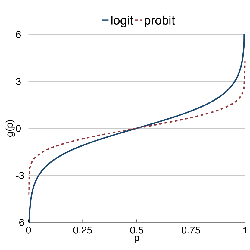
accordingly. Both link functions describe sigmoid curves smoothly and monotonically increasing from $\mu=0$ at $\bm{\beta}^{T}\mathbf{X}=-\infty$ to $\mu=1$ at $\bm{\beta}^{T}\mathbf{X}=\infty$ with the greatest rate of change occurring at $\bm{\beta}^{T}\mathbf{X}=0$, as displayed in Fig 1.

The logit function is most commonly preferred in clinical research applications where outcomes are most naturally described in terms of the odds-ratio, $\frac{p}{1-p}$ (e.g. the relationship between the odds-ratio of patient recovery/non-recovery and the concentration of an administered drug); whereas the probit function is often presented within Bayesian statistical applications exploiting an associated Gibbs sampling algorithm. Sigmoid curves such as those described by the logit and probit functions may already be seen in empirical/phenomenological astronomical models: for example, in describing the fraction of quenched galaxies as a function of mass and/or environmental density (Peng et al., 2010; Rodriguez-Puebla et al., 2014).

A reason for employing logit or probit regression to model binary response data is to obtain for objects with only $\mathbf{X}$ observations, but no observed $\mathbf{Y}$’s, the predicted probabilities that the unobserved response variable has the value 1 indicating “success”, however that is defined (e.g., ”galaxy is quenched”, ”star hosts planet”). Both models usually produce similar probabilities; though probit regression is not as commonly used for assessing the relationship of a predictor to the response since the interpretation of the exponentiated coefficient of a logit predictor as an odds ratio is a desirable feature of that model. Probit regression is normally used when a continuous variable is dichotomized so that it becomes a binary response (see Zuur et al., 2013, for an examination of these and related issues with logit and probit models from both a frequency and Bayesian perspective). It is worth noting that, while other well known machine learning algorithms (e.g., support vector machines, k-nearest neighbourhood) can be used for binary classification tasks, their main focus is prediction rather than modelling. In other words, their aim is to find a functional algorithm $f(x)$ that operates on $x$ to predict the responses $y$. GLMs, on the other hand, represent a data modelling philosophy, which assumes the sample to be generated by a stochastic process, e.g., Gamma, Poisson, with Bernoulli being the case study here. While the former may lead to a more accurate prediction for complex problems, although there are plenty of GLM extensions for such cases, the later allows a clearer interpretation of the relationship between the predictor and response variables (see §4).

Figure 1: Comparison between logit, solid blue curve and probit, dotted red curve, link functions g(p).

3.2 Maximum-likelihood estimation GLM regression with logit link function

Despite the growing popularity of Bayesian statistical analysis in the physical sciences the MLE approach to GLM fitting remains the default in the majority of statistical software packages: for this reason, and its historical significance (cf. the extensive treatment given by McCullagh and Nelder 1989), we describe this approach first.

With the likelihood of the dataset fully specified by the linear predictor, $\bm{\beta}^{T}\mathbf{X}$, and the choice of response variable distribution and link function of the GLM, the corresponding likelihood function for regression is both readily tractable and easily evaluated computationally. Iterative algorithms operating on the negative log-likelihood, such as the iteratively re-weighted least squares procedure used by glm (Venables and Ripley, 2002), thus provide a fast computational strategy for recovering the MLE solution. The output from a standard MLE GLM fitting code will typically be a list containing: (i) a MLE estimate, $\hat{{\beta}}_{i}$, for the ${\beta}_{i}$ component of each candidate predictor variable, $\mathbf{X}_{i}$; (ii) the associated estimate of its standard error, $\hat{\sigma}_{{\beta}_{i}}$, from which approximate confidence intervals (CI) on ${\beta}_{i}$ may be obtained using the Normal distribution function (e.g. a 95% CI: $\hat{{\beta}}_{i}\pm 2\hat{\sigma}_{{\beta}_{i}}$); and (iii) a $p$-value computed from the Wald test using (i) and (ii), required for significance testing of the given predictor variable. The Wald test determines how significant a predictor variable is, where for the GLM case it tests the predictor parameter values, $\hat{\beta}$, versus hypothesized values, $\beta_{0}$ (often $0$ for logistic models), and is based on MLE. The difference between $\hat{\beta}$ and $\beta_{0}$ divided by the standard error, $se$, of the residuals follows an approximate Gaussian distribution. For a specific estimate, we have

$$\frac{\hat{\beta}-\beta_{0}}{se(\hat{\beta})}\overset{.}{\sim}\mathcal{N}(0,1),$$ (7)

where $se(\hat{\beta})$ is the standard error of the estimate of $\beta$. A Wald 95% confidence interval for $\hat{\beta}$ is given by

$$\hat{\beta}\pm 1.96se(\hat{\beta}),$$ (8)

(see e.g., Pawitan, 2001; Hilbe, 2009). Estimation of (ii) is by way of the observed information matrix according to asymptotic convergence theory for MLE estimation.

In R the glm procedure may be called to perform MLE estimation of the logistic regression model using the general syntax shown in A.

3.3 Bayesian GLM regression with logit link function

The bayesglm function in the CRAN arm package is commonly used to estimate Bayesian logistic models (Gelman and Su, 2014). The code used to estimate this class of models is based on R’s default glm function (see A). Normal and Jeffreys priors have traditionally been favoured for use with continuous predictors in logit regression (e.g. Raftery 1996; Ibrahim and Laud 1991); though more recently the Cauchy has been strongly promoted as an optimal default prior (Gelman et al., 2008). It is also recommended that continuous predictors be centered if not fully standardized, if the predictor is not linearly related to the response; withal, standardizing continuous predictors help convergence, when entered into a Bayesian GLM, since it puts them on the same scale. Care must always be taken to assure that a default prior’s use with the data makes sense; to this end visual inspection of mock datasets generated from the prior–likelihood pairing unconstrained by the data can serve as an effective check. To this end “functional uniform” priors provide another means to limit prior-sensitivity in the shape of the preferred fitting function; cf. Bornkamp 2012. For the purposes of the present study we follow the Cauchy prior recommendations of Gelman et al. (2008).

3.4 Bayesian GLM regression with probit link function

Use of the probit link function for Bayesian GLM regression has become a popular choice owing to the availability of an exact Gibbs sampling algorithm for this model presented by Albert and Chib (1993). The novelty of their algorithm is a data augmentation scheme in which an additional latent variable is added for each observation having standard Normal distribution with mean set by the linear predictor, from which the likelihood of the observed response is determined according to whether or not this latent variable is above or below zero. Although the general sampler of the arm package does not in fact implement the Albert and Chib (1993) scheme, it is important to note its availability for use in more complex Bayesian hierarchical models built on the GLM framework (e.g. for the case of errors-in-variable GLM regression with binary distributions for both predictor and response variable, such as can arise in comparing the sensitivity of two alternative tests). The basic syntax for using Bayesian probit GLM in R is summarized in A. The same criteria for the use of priors that we discussed for logit models above also maintain for probit models. However, if the analyst desires to interpret the coefficients in terms of odds or risk ratios, a logit model must be used, regardless if the model is based on MLE or Bayesian methods.

4 Application to cosmological simulations

Within this section we demonstrate the application of the binomial regression techniques introduced above to answer questions from an exploratory analysis of our cosmological hydro-simulation dataset that could not be addressed by standard linear regression methods. This is because probability of occurrence for a binary outcome is bounded between 0 and 1, while the underlying theory of linear regression allows realizations with values out of this range. Rather than exhaust all possible techniques for a single dataset, our aim is to demonstrate practical differences between distinct types of binary regression: i) Bayesian vs MLE approach, both with the standard logit link (§3.2,3.3); ii) Bayesian regression comparing logit vs probit link functions (§3.3,3.4). In the first case we consider the star formation activity connection with a preselected (physically motivated) set of predictor variables: $x_{\mathrm{mol}}$ and $Z$. Alternatively, in our later analysis of the metallicity content of the galaxies, we use an automatic criterion to select the best choice of predictor variables among the entire set of halo features, or in other words the variable combination that minimizes the Akaike Information Criterion (AIC; Akaike, 1974). For all the following GLM analyses we quote the maximum likelihood (${\cal L}_{\mathrm{max}}$), the AIC as well as the alternative Bayesian Information Criterion (BIC; Schwarz, 1978).

4.1 Star formation activity

Here we discuss the connection between star formation activity and the gaseous chemical properties, $x_{\mathrm{mol}}$ and $Z$ of proto-galaxies, using a Bayesian and a MLE approach with logit link. The formation of the first metal-free stars in the Universe ended the cosmic dark ages (de Souza et al., 2011, 2012; Bromm, 2013; de Souza et al., 2013b; Whalen et al., 2013a, b) and began the production of elements heavier than lithium Maio et al. (2010, 2013); Wise et al. (2014). Thus, a key problem in physical cosmology is to understand the environmental properties of such objects (e.g., de Souza et al., 2013a; Biffi and Maio, 2013; Salvaterra et al., 2013), born out of the pristine conditions leftover by the Big Bang.

As a visual exploration, Figure 2 shows the scatter of $x_{\mathrm{mol}}$ and $Z$ coloured according to the presence of star formation activity. The objects located in the top left with high $Z$ and very low $x_{\rm mol}$ are strongly displaced from the general trend, highlighting the effects of metal enrichment of quiescent galaxies polluted by external sources. The bottom right corner is not populated because gas with large molecular fractions of $x_{\mathrm{mol}}\sim 10^{-2}$ or higher would have very short cooling times, hence would immediately form stars which pollute the surrounding medium. Therefore, the larger the deviation from the general trend, the higher the effects of feedback mechanisms.

Figure 2: Molecular fraction and gas metallicity for all haloes in the simulation, colour-coded by presence of star-formation activity: blue dots indicate no SF and red crosses indicate SF. The re-scaling and ArcSinh transformation to $Z$ is done in order to allow a better visualization of the whole range of metallicities, including the null values.

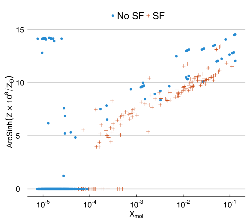
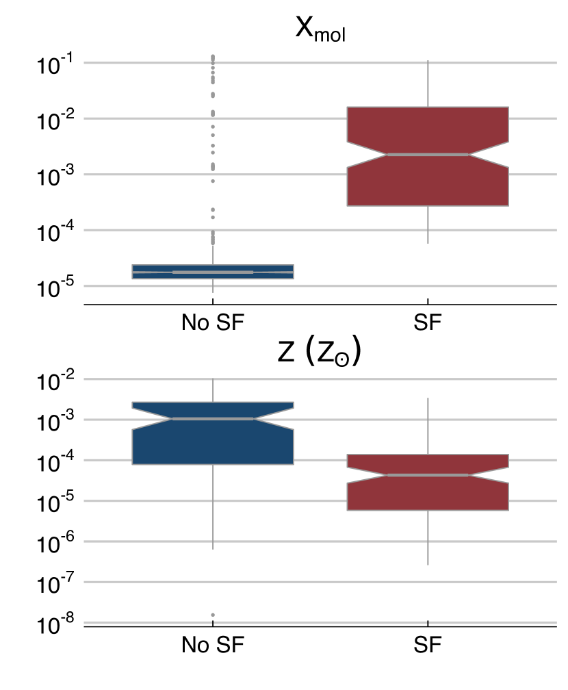
Figure 3 represents the distribution of $x_{\mathrm{mol}}$ and $Z$ colour-coded by star formation activity and displayed by a box plot. The notches represent a rough guide of the uncertainty around the median of each distribution, $\pm 1.58\times\rm{IQR}/\sqrt{n_{obj}}$, with $n_{obj}$ being the number of objects, and IQR standing for interquartile range. A visual inspection suggests that $x_{\mathrm{mol}}$ plays a major role in triggering the star formation activity, in contrast to the lower influence of $Z$ (see e.g., de Souza et al., 2014). The medians of haloes with and without star formation are different for both $x_{\mathrm{mol}}$ and $Z$, indicating they might represent different populations, which reinforce their choice as predictor variables for star formation activity.

Figure 3: Distribution of molecular fraction and metallicities for haloes colour-coded by whether they host star-formation activity or not. Red colour represents haloes with SF and blue colour haloes with no SF. The bottom and top of the box show the first and third data quartiles, while the band inside the box their median. The notches represent a rough guide of the uncertainty around the median of each distribution, $\pm 1.58\times\rm{IQR}/\sqrt{n_{obj}}$, with $n_{obj}$ being the number of objects, and IQR standing for interquartile range.

Table 2: $\hat{\beta}_{i}$ coefficients from MLE and Bayesian (with Cauchy prior) GLM logit regression analysis with $\textit{SFR}_{\rm bin}$ as the response variable and $x_{\mathrm{mol}}$ and $Z$ as predictors. The associated $p$-values ($\cal P$, see§3.2), are listed underneath the coefficients. The logarithm of the maximum likelihood (${\cal L}_{\mathrm{max}}$), the AIC and the BIC for each choice of link function are also shown.

		Response variable:
		$\textit{SFR}_{\rm bin}$
		MLE logit	Bayes logit
$\hat{\beta}_{0}$		$-2.51\pm 0.10$	$-2.50\pm 0.10$
		($\cal P\ll$ 0.001)	($\cal P\ll$ 0.001)
$\hat{\beta}_{1}$	$Z$	$-1.15\pm 0.33$	$-1.05\pm 0.27$
		$(\cal P$ = 0.0006)	$(\cal P$ = 0.0001)
$\hat{\beta}_{2}$	$x_{\mathrm{mol}}$	$1.05\pm 0.15$	$1.01\pm 0.14$
		($\cal P\ll$ 0.001)	($\cal P\ll$ 0.001)
${\cal L}_{\mathrm{max}}$		$-452$	$-452$
AIC		909	909
BIC		926	926

To perform the GLM analysis, we categorize the haloes via the binary response variable $\textit{SFR}_{\mathrm{bin}}$, as those with (SFR $>0$ ) and without (SFR = 0) star formation activity, a binary classification which makes it suitable for a binomial GLM analysis,

$$\textit{SFR${}_{\mathrm{bin}}$}=\left\{\begin{array}[]{rlr}1&\text{or `SF'~{}}&\text{if }\textit{SFR}>0,\\ 0&\text{or `no SF'~{}}&\text{if }\textit{SFR}=0.\end{array}\right.$$ (9)

The underlying properties that act as predictor variables are: $x_{\mathrm{mol}}$ and $Z$. We indicate with $p$ the probability that star formation activity is occurring in a galaxy. More specifically, $p=1$ (0) if a galaxy has (has no) star formation. The predicted probability $\pi$ is then determined by the GLM analysis and compared to observed probability $p$ (for a given decision boundary), in order to ascertain the method’s performance, as explained below. We standardized the predictors before the GLM analysis in order to ameliorate possible collinearity and scaling bias due to units differences.

Table 2 shows the estimated coefficients and related $p$-values for the various linear predictors for both Bayesian and MLE approach with the standard logit link.

The coefficients for the logit model represent the log of the odds ratio for SF activity. Since the predictors are scaled, it allows for performing a relative comparison between variables measured in different units. A one $\sigma$ increase in the halo metallicity ($\approx 8.5\times 10^{-4}Z_{\bigodot}$) produces, on average, a change of $-1.15$ in the log of odds ratio ($\approx 25\%$ in probability) for presence of SF, for an average halo with gas molecular fraction close to the mean, $x_{\rm mol}\approx 2.2\times 10^{-3}$. Likewise, for a halo with $Z\approx 1.3\times 10^{-4}Z_{\bigodot}$, an increase of $1.2\times 10^{-2}$ in $x_{\rm mol}$, increases the probability of SF by 75%. The analysis not only confirms $x_{\rm mol}$ as a critical parameter to trigger the SF in primordial halos, in agreement with previous works (see e.g, de Souza et al., 2014), but provides the means to interpret the role of each halo property in terms of odds and probabilities. As stated in §3, the GML analysis provides an estimate $\hat{\beta}_{i}$ for the $\beta_{i}$ component of each predictor variable. The values obtained can be used to calculate the linear predictor, $\eta$:

$$\eta=\hat{\beta}_{0}+\hat{\beta}_{1}Z+\hat{\beta}_{2}x_{\mathrm{mol}},$$ (10)

and transformed into a predicted probability, $\pi$:

$$\pi=\frac{e^{\eta}}{1+e^{\eta}},$$ (11)

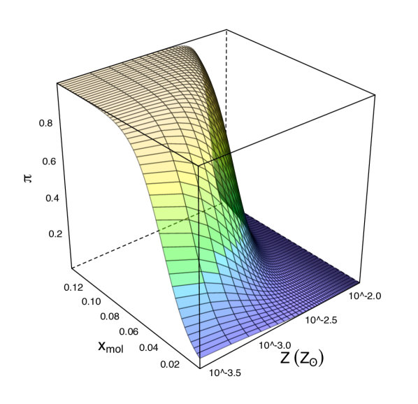
which uses the logit link defined in Eq. 3. Figure 4 displays the regression plane solution using the logit link. The surface gives the probability of SF activity for each pair ($Z$, $x_{\rm mol}$).

Figure 4: Predicted probabilities, $\pi$, of star formation activity vs metallicity, $Z$, and molecular fraction, $x_{\rm mol}$, for the logit regression.

This can be used to assign a class membership for each object for a given probability decision threshold, $\pi_{th}$, i.e. SF = 1 if $\pi>\pi_{th}$ and 0 if $\pi<\pi_{th}$. For each halo, the predicted probability can be compared to the observed probability, which in this case is $p$ = 1 if the halo presents star formation activity, and $p$ = 0 otherwise. The performance of the method in reproducing the correct observed probabilities can be evaluated as detailed in §5. When class sample sizes are approximately equal, which in this scenario would imply a similar number of galaxies with and without star formation activity, the optimal decision threshold is $\pi_{th}\sim 0.50$ (see §5.2).

Nevertheless, this criterion is not appropriate when the class sizes are imbalanced and an adjusting decision threshold has to be used. As a trivial example, if the data is imbalanced, the fit can predict $\pi=0.2$ for all haloes with SF = 1 and $\pi=0.1$ for all haloes with SF = 0. In this hypothetical scenario, the decision boundary would be in the range 0.1-0.2, instead of being 0.5 (50%) as one would naively expect. A more detailed explanation of how to adjust the decision threshold probability, $\pi_{th}$, and a discussion of the predictive power of the method is given in §5.

The MLE and Bayesian approaches give almost identical results for the estimated coefficients $\hat{\beta_{i}}$, despite the addition of the prior. It seems that there is no preferred model, as indicated also by the comparison between the corresponding AIC, BIC and the logarithm of maximum likelihood ${\cal L}_{\mathrm{max}}$. We note though the smaller credible intervals from the Bayesian logit in comparison to those from the MLE analysis.

4.2 The Pop III-Pop II/I dichotomy

As previously mentioned, the first generation of stars (Pop III) are thought to form within pristine gas, while standard Pop II/I star formation takes place within metal enriched gas. Here we investigate the Pop III-Pop II/I dichotomy using a Bayesian regression with logit and probit link functions.

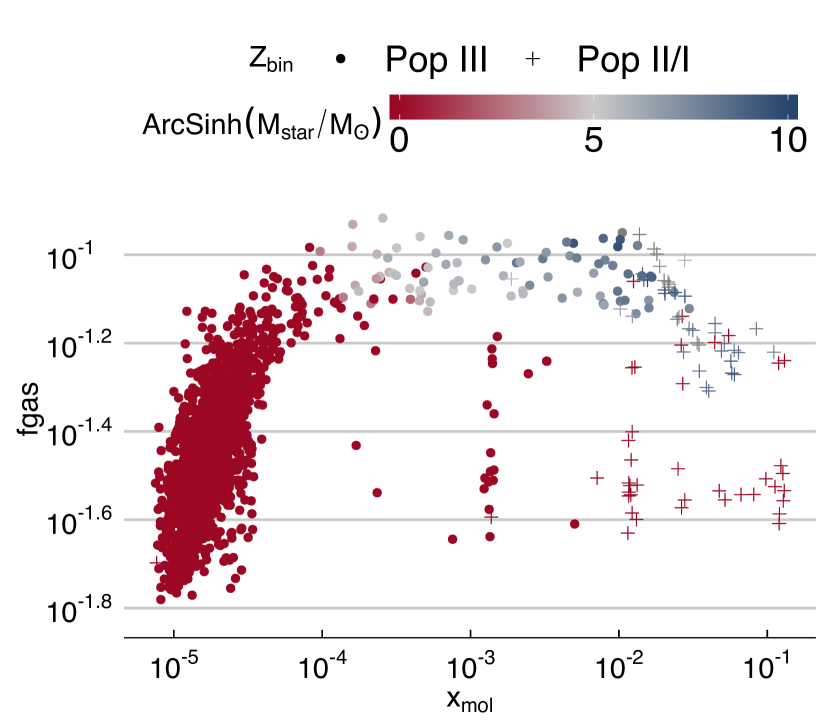
Figure 5 shows the gas fraction versus molecular fraction with a colour scheme corresponding to stellar mass. A visual inspection indicates that larger molecular fractions are strongly associated with high-metallicity environments, confirming that the molecular fraction is the main predictor. From a physical point of view, the fact that the gas fraction in the environment of Pop II/I stars is usually lower than that of Pop III stars suggests that the cosmological production of early heavy elements enhances significantly gas cooling capabilities and boosts molecule formation in polluted material well above $x_{\rm mol}\sim$ a few percents. Basically, metal cooling allows gas fragmentation at regimes where pristine material is not able to condense – see the region: { $x_{\rm mol}>10^{-2}$, $f_{\rm gas}<10^{-1.1}$ }.

The present cosmological simulations switch the stellar IMF from top-heavy to standard Salpeter when the metallicity exceeds $Z_{\rm crit}=10^{-4}Z_{\bigodot}$ (see §2). To perform the GLM analysis in this section, we define $Z_{\mathrm{bin}}$ as the binary response variable, depending on whether the gas metallicity lies above or below $Z_{\rm crit}$:

$$Z_{\mathrm{bin}}=\left\{\begin{array}[]{rl}1&\text{or `Pop II/I'~{}}\text{if }Z\geq Z_{\rm crit},\\ 0&\text{or `Pop III'~{}}\text{if }Z<Z_{\rm crit}.\end{array}\right.$$ (12)

One can then use the binomial GLM regression to determine which global galaxy properties are linked to the dichotomy between the Pop II/I and Pop III host environment and how. We also use this problem as an opportunity to demonstrate the use of both logit ($\eta=\log\pi/(1-\pi)$) and probit ($\eta=\Phi^{-1}(\pi)$) link functions. Likewise the previous section, $\pi$ here represents the predicted probability for the success of the binary response variable, in other words if a galaxy halo is an enriched Pop II/I environment given the underlying galaxy properties.

Firstly, one must identify the key galaxy properties as predictor variables. As in the previous example, we scale the predictors by their respective means and divide by the standard deviations before performing the analysis. Nonetheless, rather than adding a set of pre-chosen predictors, we herein illustrate a general feature selection approach, making use of step function in R. The method attempts to alternately drop and add members of an input set of predictor candidates in order to minimize the AIC of the fitted model. By using the stepwise algorithm we are able to select the most parsimonious combination of parameters and interaction terms from our input set. The scheme employed here falls into the category of wrapper methods of feature selection, but there exist other approaches that can be tailored to determine how relevant a feature is in representing a class in a high-dimensional space, i.e. so-called filter methods (see e.g., Donalek et al., 2013, for a review of feature selection methods in astronomy).

Figure 5: Scaled gas fraction versus molecular fraction, color-coded by stellar mass transformed by ArcSinh for visual purposes. Circles and crosses represent pristine/low-metallicity Pop III and high-metallicity Pop II/I stellar environments, respectively.

Table 3: $\hat{\beta}_{i}$ coefficients from results of a Bayesian GLM analysis (with Cauchy prior) with logit and probit links. $Z_{\mathrm{bin}}$, is the response variable, while the intercept $\hat{{\beta}}_{0}$, $x_{\mathrm{mol}}$, $f_{\mathrm{gas}}$, $M_{\mathrm{star}}$ and $M_{\rm star}/M_{\mathrm{gas}}$  are predictors. The associated $p-values$ ($\cal P$) are listed underneath the coefficients. The logarithm of the maximum likelihood (${\cal L}_{\mathrm{max}}$), the AIC and the BIC for each choice of link function are also shown.

		Response variable:
		$Z_{\mathrm{bin}}$
		Logit link	Probit link
$\hat{{\beta}}_{0}$		$-3.76\pm 0.22$	$-$1.94$\pm 0.09$
		($\cal P\ll$ 0.0001)	($\cal P\ll$ 0.0001)
$\hat{\beta}_{1}$	$x_{\mathrm{mol}}$	5.90$\pm$0.65	2.91 $\pm$ 0.32
		($\cal P\ll$ 0.0001)	($\cal P\ll$ 0.0001)
$\hat{\beta}_{2}$	$f_{\mathrm{gas}}$	$-0.97\pm 0.27$	$-0.43\pm 0.12$
		($\cal P$=0.0004)	($\cal P$=0.0004)
$\hat{\beta}_{3}$	$M_{\rm star}$	$0.80\pm 0.33$	$0.54\pm 0.22$
		($\cal P$=0.02)	($\cal P$=0.01)
$\hat{\beta}_{4}$	$M_{\rm star}/M_{\mathrm{gas}}$	$-0.86\pm 0.41$	$-0.58\pm 0.23$
		($\cal P$=0.04)	($\cal P$=0.01)
${\cal L}_{\mathrm{max}}$		$-$113	$-$114
AIC		236	238
BIC		263	265

We found that $x_{\mathrm{mol}}$ plays the most important role in the predictive power of the model. Furthermore, the factors that maximise the information gain and are worth including as predictor parameters are: $x_{\mathrm{mol}}$, $f_{\mathrm{gas}}$, $M_{\rm star}/M_{\mathrm{gas}}$, and $M_{\mathrm{star}}$. The selection is equivalent regardless of whether the logit or probit link functions are used.

Having chosen suitable input variables, we can then apply the GLM analysis as described in §3.3 and §3.4. In Table 3 we provide the estimated coefficients for the predictor variables and respective $p-values$. The coefficients in the two cases are different as can be seen in Table 3, which is mostly a consequence of the different choices of link function. Likewise, as in section 4.1, the logit coefficients can be associated with probabilities. Once more, $x_{\mathrm{mol}}$ stands as the most influential variable, and a variation of $\approx 1.2\times 10^{-2}$ in $x_{\mathrm{mol}}$, increases the chances for an average dark halo to be a potential host of Pop II/I stars by a factor of 99.7%. The predicted probabilities $\pi$ are therefore estimated by solving the following equation:

$$\eta = \hat{\beta}_{0}+\hat{\beta}_{1}x_{\mathrm{mol}}+\hat{\beta}_{2}f_{\mathrm{gas}}+$$

$$+ \hat{\beta}_{3}M_{\mathrm{star}}+\hat{\beta}_{4}\frac{M_{\rm star}}{M_{\rm gas}},$$

as well as either

$$\Phi^{-1}(\pi) = \eta,$$ (14)

if the probit link function (Eq. 4) is used, or

$$\pi = \frac{e^{\eta}}{1+e^{\eta}},$$ (15)

for the logit link function (Eq. 3).

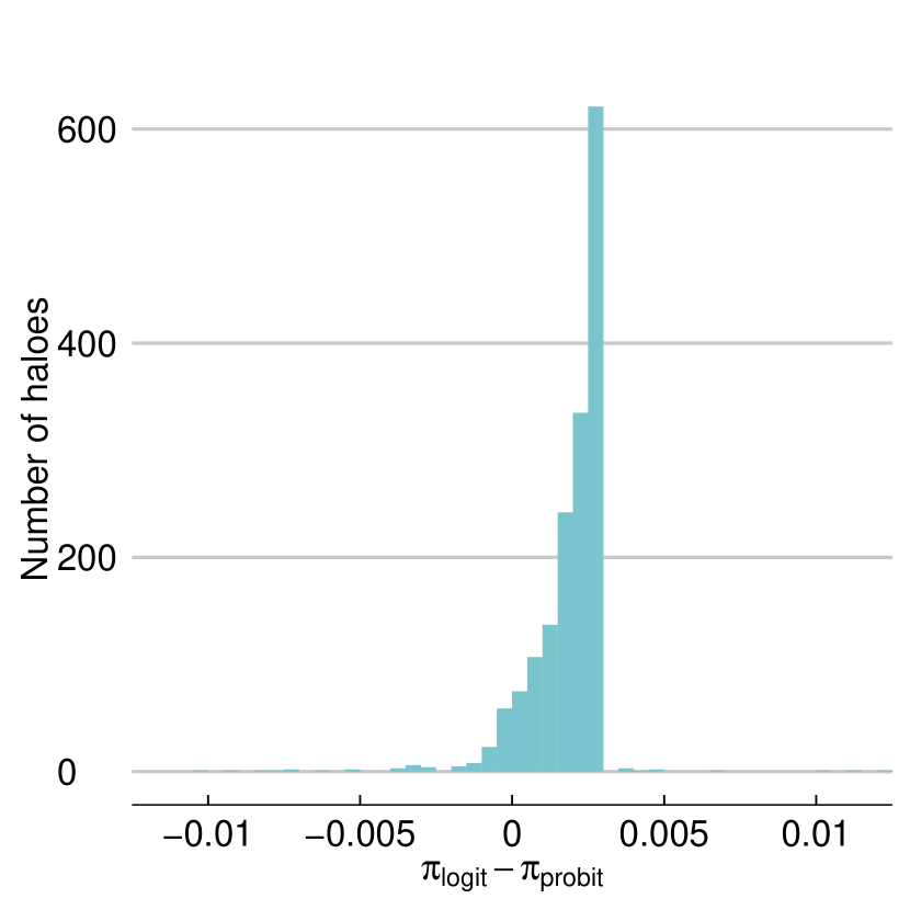
Ultimately, logit and probit regression result in similar predictions for the probability that the response variable is unity, i.e. $\pi_{\mathrm{logit}}\approx\pi_{\mathrm{probit}}$. To illustrate this point, we calculate $\pi$ twice for each galaxy in our sample given its underlying properties: once using the logit link and then again using the probit link. A histogram of the differences is shown in Figure 6. The logit link function leads to a value of $\pi$ that is only slightly higher. Thus, for the case studied here, both link functions generate similar predictions, in spite of their different interpretations (see e.g., Zuur et al., 2013). A quantitative comparison between the predictive power of logit and probit, and the increase in number of relevant predictor variables are given in the following section.

Figure 6: Histogram of the difference between predicted probabilities from logit, $\pi_{\rm logit}$, and probit $\pi_{\rm probit}$, regressions.

5 Diagnostics

We now describe our experimental setting to assess the performance of GLM on the prediction of star formation activity $\textit{SFR}_{\rm bin}$ and metal enrichment $Z_{\rm bin}$. We report on accuracy (i.e., fraction of events correctly classified) using a resampling technique known as $10$-fold cross validation (Hastie et al., 2009) in §5.1, on Receiver Operating Characteristic (ROC) curves (Duda et al., 2000) in §5.2 and on the confusion matrix in §5.3.

5.1 Cross validation

When assessing model performance, it is of utmost importance to set aside a validation set to estimate the true generalization power of the model under analysis. This is particularly relevant to avoid the risk of model over-fitting. An over-fitted model captures aberrations on the training set that render the model useless during prediction. A popular approach to model validation makes use of resampling techniques Hastie et al. (2009).

In the resampling technique known as $k$-fold cross validation, the data is divided into $k$ folds (subsamples) of equal size. The technique runs iteratively as follows. On each iteration, $k-1$ folds are used for training (model fitting), while the remaining fold is used for testing (model assessment). The procedure repeats $k$ times, using mutually exclusive testing folds across iterations. The final result is the average over the score obtained on each iteration. Cross validation estimates the true performance of a classifier by exploiting all available information. In our experiments, we use a value of $k=10$ to achieve a trade-off between bias (proportional to $k$) and variance (inversely proportional to $k$). Hereafter, all ROC curves and confusion matrices are estimated using the $k=10$ cross-validation approach.

5.2 ROC curves

ROC curves provide both a visually and quantitative approach to report on the accuracy of predictions for binary classifiers. Hereafter, we refer to the classifications as positive (1) or negative (0). The technique consists of plotting the true positive rate (TPR or Sensitivity) vs the false positive rate (FPR or Specificity) as we vary the decision boundary $\pi_{th}$. The variation in the decision boundary enables us to assess the performance of the classifier under unequal error costs (i.e., under scenarios where the cost of a false positive is different from a false negative).

Specifically, to generate a ROC curve we make use of two measurements:

$$\rm{Sensitivity} = \frac{\rm TP}{\rm TP+FN};$$

$$\rm{Specificity} = \frac{\rm TN}{\rm TN+FP},$$ (16)

where TP = true positives, FP = false positives, TN = true negatives, and FN = false negatives. For example, in the case studied in §4.1 we would have:

• TP: the galaxy has SF and the method predicts SF,

• FP: the galaxy does not have SF but the method predicts SF,

• TN: the galaxy does not have SF and the method predicts no SF,

• FN: the galaxy has SF, but the method predicts no SF.

In this case the Sensitivity (Specificity) would quantify the ability of the method to correctly identify galaxies with (without) SF: the closer to 1 these values are, the more successful the analysis is. The same interpretation holds for the case discussed in §4.2 by replacing $\textit{SFR}_{\rm bin}$ with $Z_{\rm bin}$.

Sensitivity is normally plotted on the $y$-axis, while $1-$ Specificity is plotted on the $x$-axis (Figs. 7 and 8). The classifier is run several times with a different value of the decision threshold; each run provides a point in the (1-Specificity, Sensitivity) plane. The corresponding true ROC curve is obtained by joining the set of coordinates starting at (0,0) and ending at (1,1). An ideal ROC curve goes from (0,0) to (0,1) to (1,1). A quantitative approach to assess the quality of a ROC curve is to calculate the area under the curve (AUC), as a fraction of the area under the ideal curve, as often done in cases of discrepancy or inequality measurements (since e.g. Gini, 1912, 1921). Higher values of AUC correspond to more accurate classifiers, while a value of 0.5 corresponds to a random classifier (Hilbe, 2009).

The ROC curve can be used to access the optimal $\pi_{th}$, which is a trade-off between Sensitivity and Specificity. In order words, it is the one corresponding to the coordinate with minimum distance from (0,1), where both Sensitivity and Specificity are maximum. This is essential to ultimately assign a class membership for each data. A visual analysis of this classification scheme is made via the confusion matrix, which will be discussed in the next section.

5.3 Confusion Matrix

A complementary diagnostics method is the confusion matrix $C$, which captures information about the actual and predicted classifications of a particular learning algorithm or classifier (Kohavi and Provost, 1998). Columns in $C$ correspond to actual classes, whereas rows correspond to predicted classes (e.g., $\textit{SFR}_{\rm bin},Z_{\rm bin}$). The diagonal elements of the matrix contain the number of cases where the actual and predicted class agree, e.g., $C(i,i)$ contains the number of cases where class $i$ was predicted correctly. Off-diagonal elements capture all combination of misclassifications, e.g., $C(i,j)$ with $i\neq j$ contains the number of cases where class $i$ was incorrectly predicted as class $j$. On a $2\times 2$ confusion matrix, entries along the diagonal stand for the number of true negatives TN (top left) and true positives TP (bottom right). Specifically, $C$ can be represented as follows:

$$\begin{array}[]{c|c}\rm TN&\rm FN\\ \hline\cr\rm FP&\rm TP\\ \end{array}.$$ (17)

6 Performance Comparison

During this section we compare the predictive performance of both logit vs probit links as discussed in §4.2 and between GLMs and artificial networks for the case discussed at §4.1.

6.1 Logit vs Probit

Figure 7: Left panel: ROC curves for logit (solid blue curve) vs probit (dotted orange curve) regression in the case discussed in §4.2. Right panel: ROC curves for logit regression for different combinations of predictor variables: $\sim\hat{\beta_{0}}$ (dotted-dashed green curve); $\sim\hat{\beta_{0}}+\hat{\beta_{4}}\frac{M_{\rm star}}{M_{\rm gas}}$ (dashed-dashed gold curve); $\sim\hat{\beta_{0}}+\hat{\beta_{4}}\frac{M_{\rm star}}{M_{\rm gas}}+\hat{\beta_{3}}M_{\rm star}$ (dotted magenta curve); $\sim\hat{\beta_{0}}+\hat{\beta_{4}}\frac{M_{\rm star}}{M_{\rm gas}}+\hat{\beta_{3}}M_{\rm star}+\hat{\beta_{2}}f_{\rm gas}$ (dashed cyan curve); $\sim\hat{\beta_{0}}+\hat{\beta_{4}}\frac{M_{\rm star}}{M_{\rm gas}}+\hat{\beta_{3}}M_{\rm star}+\hat{\beta_{2}}f_{\rm gas}+\hat{\beta_{1}}x_{\rm mol}$ (solid blue curve). The dotted grey curve in both figures represents the performance of a random classifier.

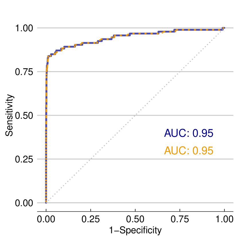
The left panel of Figure 7 shows a comparison between logit and probit ROC curves, pointing to the equivalence in predictive power of both methods, achieving an outstanding performance of AUC = 0.95, although their coefficients have a different interpretation.

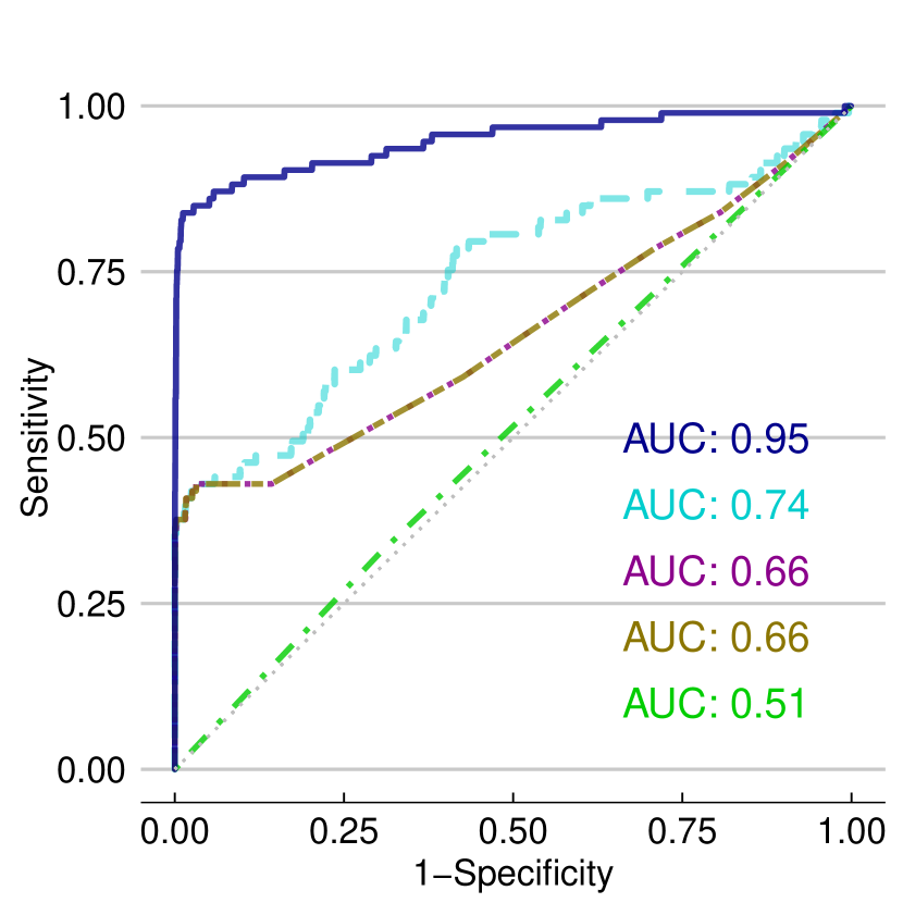
In order to assess the relevance of a good set of predictor variables, the right panel of Figure 7 shows a visualization of the logit GLM regression obtained adding different predictor variables. While $f_{\rm gas}$, $M_{\rm star}$, and $M_{\rm star}/M_{\rm gas}$ together have a non-negligible contribution to explain the metallicity enrichment above/below $Z_{\rm crit}$ with an AUC = 0.74, the molecular fraction, $x_{\rm mol}$, clearly stands out as the most important parameter. This suggests that the level of molecular gas fraction has a strong connection with the level of metal content in primordial haloes.

6.2 Comparison between GLM and Neural Networks

We compare GLM with a popular non-parametric technique to classification known as Artificial Neural Networks (ANN) (Duda et al., 2000). A nonlinear multi-layer ANN is capable of expressing flexible decision boundaries over the variable space; it is a nonlinear statistical model that applies to both regression and classification. In particular, for an ANN with one hidden layer, each intermediate and output node computes a weighted combination of inputs, compressed (squashed) by a sigmoid (nonlinear) function (Bishop, 1996).

Figure 8 shows ROC curves for GLM and ANN analysis of the case presented in §4.1. The ROC curves were generated as those discussed in the previous section. In our experiments, GLM attains an AUC slightly higher than that of ANN (0.87 versus 0.83), reinforcing our claim for the competitiveness of GLM despite its inherent simplicity. We stress that the above comparison should not be extrapolated to imply that GLMs are better suited for binary classification prediction than ANNs, but for this particular and somewhat simple problem, both are equally good. The main advantages of GLMs are their portability and interpretation of the coefficients. Moreover, the possibility to approach the problem from a Bayesian perspective is extremely beneficial when dealing with inherent issues of observational data, such as errors-in-variables, selection bias, etc (Loredo, 2013).

Figure 8: ROC curves for Generalized Linear Model (solid blue curve) and Artificial Neural Network (dashed green curve) for the case discussed in §4.1. The dotted grey curve represents the performance of a random classifier.

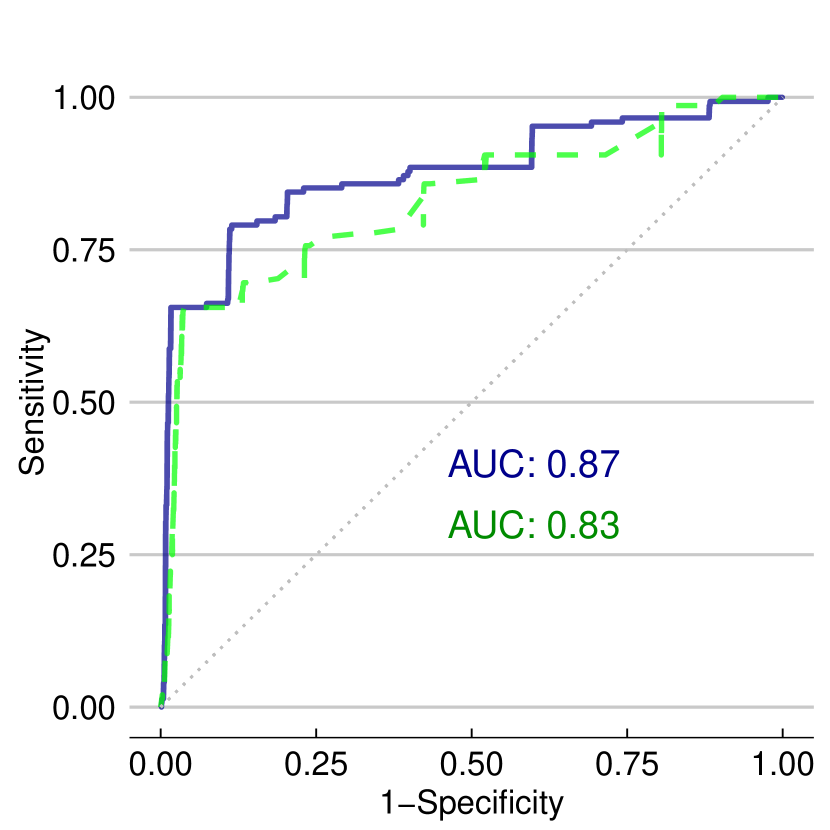
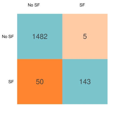
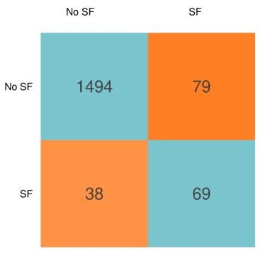
Figure 9 shows two confusion matrices, one for GLM (left) and one for ANN (right) for the case underlined in §4.1, i.e. the connection between star formation activity and the gaseous chemical properties $x_{\mathrm{mol}}$ and $Z$ of galaxies. While TN is similar under both classifiers, TP differs significantly: ANN exhibits a high number of false negative FN (upper right) in contrast to the corresponding entry for GLM. Hence, the overall accuracy of GLM is $96.7\%$, while that of ANN is $93\%$.

Figure 9: Confusion matrix for the model SFR${}_{\mathrm{bin}}\sim x_{\mathrm{mol}}+Z$ (in R notation) discussed in §4.1, as expected by logistic GLM (left) and ANN (right). In each panel, the first and second columns refer to the simulated objects with (1532 galaxies) and without (148 galaxies) star formation activity, respectively. The on-diagonal elements refer to TN (top left) and TP (bottom right), while the off-diagonal elements refer to FP (top right) and FN (bottom left).The color scheme ranges from blue, correct values, to orange, incorrect values, with the intensity determined by the number of objects in each category.

7 Conclusions

We perform a comprehensive introduction of logit and probit generalized linear model regression for the astronomical community from both a maximum likelihood and a Bayesian perspective. As a real application, we analyse the host environment of the first generation of stars as predicted by numerical hydro-simulations of the early Universe, including detailed chemistry, gas physics, star formation, stellar evolution and stellar feedback. A summarizing flowchart visualization of the entire process is given in B.

The halo properties analysed here are categorical with two possible outcomes and therefore ideal candidates for the application of binomial GLM regression. These correspond to either (i) the presence/absence of star formation activity, or (ii) metal content above/below the critical metallicity associated to stellar population transition in primordial epochs.

In the first case, the explanatory variables were decided beforehand with preliminary physical motivation, while in the second case, we demonstrated the use of the AIC to select the most parsimonious set of variables from among a given set of candidates. This method is particularly beneficial for providing new insight into fundamental underlying galaxy properties.

A maximum likelihood as well as a Bayesian (with Cauchy priors) analysis result in very similar coefficients for each variable. We have explored the use of both logit and probit link functions and found that they lead to different $\hat{\beta}$ coefficients, but with the same sign. Nevertheless, calculations of the predicted probabilities produce very similar results regardless of whether a logit or probit model is used for estimation.

The GLM method has been shown to be very competitive against artificial neural networks, attaining an area under the curve (AUC) coefficient of 0.87 against 0.83 from ANN. Since a value of $\rm AUC=1$ indicates a perfect classifier and a value of $\rm AUC=0.5$ suggests a random predictor, both GLM and ANN approaches can be considered rather robust, albeit the AUC seems to favour slightly the GLM for this particular test. Furthermore, given its inherently simplicity, GLM results are easily portable and have a more straightforward interpretation of its coefficients in terms of odds and probabilities.

Also worth noting is that the potential of GLM regression goes far beyond binary classification. Many data situations involve discrete data, but are nevertheless modelled as if the response variable were continuous. If the data are modelled as discrete, it is by employing a Poisson model, without due regard for the corresponding distributional assumption of equality between mean and variance (equidispersion). This is a strongly restrictive technical assumption and is rarely met in real data. In practice, there are nearly as many count models as there are shapes of counts: there is a variety of mixture models, of zero-inflation models, of two-part hurdle models, of finite mixture models, etc. which assume that the counts being modelled are being generated from more than one source. There are situation where the classic GLM assumption of uncorrelated measurements fails, e.g., for repeated measurements from the same object. For theses cases, plenty of extensions exist, such as generalized estimating equations (Liang and Zeger, 1986). Additionally, there are generalized additive models, non-parametric quantile count models, models with endogenous stratification, panel models, and 3-parameter count models, to name only a few. GLMs are of common use in the statistical literature, but almost Terra incognita in astronomical data analysis, with only few recent notable applications of logistic regression (e.g. Raichoor and Andreon 2012, 2014; Lansbury et al. 2014), Poisson regression (e.g. Andreon and Hurn 2010) and negative binomial regression (Ata et al., 2015).

Finally, we highlight the vast potential of GLMs and extended GLMs for the astronomical community through their possible application to a plethora of astronomical problems, such as: photometric redshift estimation (gamma distributed data; Elliott et al., 2015), globular cluster counts (Poisson distributed data), or galaxy morphological classification (multinomial distributed data). GLMs might be a precious instrument for astronomical investigations, thanks to their capabilities in addressing scientific questions that could not be answered otherwise. Thus, we are confident in a prompt integration of these methods into astronomy, with the hope that contemporary statistical techniques may become common practice in the $\rm 21^{st}$ century astrophysical research.

Appendix A R scripts

In the following, we display the R scripts for the models discussed in sections 3.2,3.3, and 3.4, respectively.

MLE with logit link

The basic syntax for a MLE logit model:

⬇

1 glm.fit <- glm(y~x1+x2+…,

2 family = binomial("logit")).

The summary command can be called on the glm.fit object returned, as can plot which will display a number of useful fit and model checking diagnostics.

Bayesian GLM with logit link

The basic syntax for a Bayesian logit model:

⬇

1 library(arm)

2 #Output identical to ML logit

3 blr1 <- bayesglm(y ~ x1+x2+ …,

4 family=binomial(link="logit"),

5 prior.scale=Inf, prior.df=Inf,

6 data=<datafile>)

7 display(blr1)

8

9 #Bayes GLM with default binomial

10 #logit link and Cauchy prior

11 #with scale=2.5

12

13 blr2 <- bayesglm(y~x1+x2+…,

14 family=binomial,

15 data=<datafile>)

16 display(blr2)

17

18 #Bayes logit with normal prior

19 #with scale=2.5

20 blr3 <- bayesglm(y~x1+x2+…,

21 family=binomial,

22 prior.scale=2.5, prior.df=Inf,

23 data=<datafile>)

24 display(blr3).

Bayesian GLM with probit link

The basic syntax for a Bayesian probit model:

⬇

1 library(arm)

2 bpr <- bayesglm(y~x1+x2+…,

3 family=binomial(link="probit"),

4 prior.scale=2.5, prior.df=Inf,

5 data=<datafile>)

6 display(bpr).

Appendix B Flowchart for GLM regression

This section illustrates a brief summary of GLM analysis and model diagnostics. It comprises:

• Acquire the dataset.

• Choose the response variable to be modelled.

• Choose predictor variables.

• Choose GLM family, e.g. Gaussian, Poisson, binomial.

• Choose either a maximum-likelihood or a Bayesian approach.

• Choose link function.

• Estimating coefficients by means of a GLM or Bayesian GLM analysis, i.e., estimate $\eta$ and predicted probabilities $\pi$

• Classification and diagnostic tests:

  • ROC curve-probability threshold.

  • Confusion Matrix for a given $\pi_{th}$ and assigned class memberships.

Figure 10: Tabular data is represented by blue rectangles, calculations by red diamonds, choices by green parallelograms, and diagnostic outcomes by orange heptagons.

References

- Akaike (1974) Akaike, H., December 1974. A new look at the statistical model identification. IEEE Transactions on Automatic Control 19 (6), 716–723.
- Albert (2007) Albert, J., 2007. Bayesian computation with R. Vol. 747389981. Springer.
- Albert and Chib (1993) Albert, J. H., Chib, S., 1993. Bayesian analysis of binary and polychotomous response data. Journal of the American Statistical Association 88 (422), 669–679.
- Andreon and Hurn (2010) Andreon, S., Hurn, M. A., Jun. 2010. The scaling relation between richness and mass of galaxy clusters: a Bayesian approach. MNRAS404, 1922–1937.
- Ata et al. (2015) Ata, M., Kitaura, F.-S., Müller, V., Feb. 2015. Bayesian inference of cosmic density fields from non-linear, scale-dependent, and stochastic biased tracers. MNRAS446, 4250–4259.
- Biffi and Maio (2013) Biffi, V., Maio, U., Dec. 2013. Statistical properties of mass, star formation, chemical content and rotational patterns in early z 9 structures. MNRAS436, 1621–1638.
- Bishop (1996) Bishop, C. M., 1996. Neural Networks for Pattern Recognition. Oxford University Press, 1st Edition.
- Bornkamp (2012) Bornkamp, B., 2012. Functional uniform priors for nonlinear modeling. Biometrics 68 (3), 893–901.
- Breslow and Clayton (1993) Breslow, N. E., Clayton, D. G., 1993. Approximate Inference in Generalized Linear Mixed Models. Journal of the American Statistical Association 88 (421), 9–25.
- Bromm (2013) Bromm, V., Nov. 2013. Formation of the first stars. Reports on Progress in Physics 76 (11), 112901.
- Bromm et al. (2001) Bromm, V., Ferrara, A., Coppi, P. S., Larson, R. B., Dec. 2001. The fragmentation of pre-enriched primordial objects. MNRAS328, 969–976.
- Cameron (2011) Cameron, E., 1 2011. On the estimation of confidence intervals for binomial population proportions in astronomy: The simplicity and superiority of the bayesian approach. Publications of the Astronomical Society of Australia 28, 128–139.
-
de Jong and Heller (2008)
de Jong, P., Heller, G. Z., 2008. Generalized Linear Models for Insurance Data.
Cambridge University Press, cambridge Books Online.
URL http://dx.doi.org/10.1017/CBO9780511755408 - de Souza et al. (2013a) de Souza, R. S., Ciardi, B., Maio, U., Ferrara, A., Jan. 2013a. Dark matter halo environment for primordial star formation. MNRAS428, 2109–2117.
- de Souza et al. (2013b) de Souza, R. S., Ishida, E. E. O., Johnson, J. L., Whalen, D. J., Mesinger, A., Dec. 2013b. Detectability of the first cosmic explosions. MNRAS436, 1555–1563.
- de Souza et al. (2012) de Souza, R. S., Krone-Martins, A., Ishida, E. E. O., Ciardi, B., Sep. 2012. Searching for the first stars with the Gaia mission. A&A545, A102.
- de Souza et al. (2014) de Souza, R. S., Maio, U., Biffi, V., Ciardi, B., May 2014. Robust PCA and MIC statistics of baryons in early minihaloes. MNRAS440, 240–248.
- de Souza et al. (2011) de Souza, R. S., Yoshida, N., Ioka, K., Sep. 2011. Populations III.1 and III.2 gamma-ray bursts: constraints on the event rate for future radio and X-ray surveys. A&A533, A32.
- Diggle et al. (2002) Diggle, P., Moyeed, R., Rowlingson, B., Thomson, M., 2002. Childhood malaria in the gambia: a case-study in model-based geostatistics. Journal of the Royal Statistical Society: Series C (Applied Statistics) 51 (4), 493–506.
- Donalek et al. (2013) Donalek, C., Djorgovski, S., Mahabal, A., Graham, M., Drake, A., Fuchs, T., Turmon, M., Arun Kumar, A., Philip, N., Yang, M.-C., Longo, G., Oct 2013. Feature selection strategies for classifying high dimensional astronomical data sets. In: Big Data, 2013 IEEE International Conference on. pp. 35–41.
- Doss and Narasimhan (1994) Doss, H., Narasimhan, B., 1994. Bayesian poisson regression using the gibbs sampler: Sensitivity analysis through dynamic graphics. Tech. rep., Technical report, Penn State Erie.
- Duda et al. (2000) Duda, R., Hart, P. E., Stork, D. G., 2000. Pattern Classification. Wiley-Interscience, 2nd. Edition.
- Elliott et al. (2015) Elliott, J., de Souza, R. S., Krone-Martins, A., Cameron, E., Ishida, E. E. O., Hilbe, J., Apr. 2015. The overlooked potential of Generalized Linear Models in astronomy-II: Gamma regression and photometric redshifts. Astronomy and Computing 10, 61–72.
- Gelman et al. (2008) Gelman, A., Jakulin, A., Pittau, M. G., Su, Y.-S., 2008. A weakly informative default prior distribution for logistic and other regression models. The Annals of Applied Statistics, 1360–1383.
Gelman and Su (2014)
Gelman, A., Su, Y.-S., 2014. arm: Data Analysis Using Regression and
Multilevel/Hierarchical Models. R package version 1.7-05.
URL http://CRAN.R-project.org/package=arm - Gini (1912) Gini, C., 1912. Variabilitá e mutabilitá. Memorie di metodologica statistica (Ed. Pizetti E, Salvemini, T).
- Gini (1921) Gini, C., 1921. Measurement of inequality of incomes. The Economic Journal 31 (121), 124–126.
- Griswold et al. (2004) Griswold, M., Parmigiani, G., Potosky, A., Lipscomb, J., 2004. Analyzing health care costs: a comparison of statistical methods motivated by medicare colorectal cancer charges. Biostatistics 1 (1), 1–23.
- Hardin and Hilbe (2012) Hardin, J. W., Hilbe, J. M., 2012. Generalized Linear Models and Extensions, 3rd Edition, 3rd Edition. StataCorp LP.
- Hastie and Tibshirani (1986) Hastie, T., Tibshirani, R., 1986. Generalized additive models. Statistical science, 297–310.
- Hastie et al. (2009) Hastie, T., Tibshirani, R., Friedman, J., 2009. The Elements of Statistical Learning: Data Mining, Inference, and Prediction. Springer, 2nd. Edition.
- Hilbe (2014) Hilbe, J., 2014. Modeling Count Data. Cambridge University Press.
Hilbe (2009)
Hilbe, J. M., 2009. Logistic Regression Models. Chapman & Hall/CRC Texts in
Statistical Science. Taylor & Francis.
URL http://books.google.es/books?id=eJcMIAAACAAJ - Hubble (1929) Hubble, E., 1929. A relation between distance and radial velocity among extra-galactic nebulae. Proceedings of the National Academy of Sciences 15 (3), 168–173.
Ibrahim and Laud (1991)
Ibrahim, J. G., Laud, P. W., 1991. On bayesian analysis of generalized linear
models using jeffreys’s prior. Journal of the American Statistical
Association 86 (416), pp. 981–986.
URL http://www.jstor.org/stable/2290514 - Isobe et al. (1990) Isobe, T., Feigelson, E. D., Akritas, M. G., Babu, G. J., 1990. Linear regression in astronomy. The Astrophysical Journal 364, 104–113.
- Kohavi and Provost (1998) Kohavi, R., Provost, F., 1998. Glossary of terms. Machine Learning 30 (2-3), 271–274.
- Komatsu et al. (2011) Komatsu, E., Smith, K. M., Dunkley, J., Bennett, C. L., Gold, B., Hinshaw, G., Jarosik, N., Larson, D., Nolta, M. R., Page, L., Spergel, D. N., Halpern, M., Hill, R. S., Kogut, A., Limon, M., Meyer, S. S., Odegard, N., Tucker, G. S., Weiland, J. L., Wollack, E., Wright, E. L., Feb. 2011. Seven-year Wilkinson Microwave Anisotropy Probe (WMAP) Observations: Cosmological Interpretation. ApJS192, 18.
- Lansbury et al. (2014) Lansbury, G. B., Lucey, J. R., Smith, R. J., 2014. Barred s0 galaxies in the coma cluster. Monthly Notices of the Royal Astronomical Society 439 (2), 1749–1764.
- Liang and Zeger (1986) Liang, K.-Y., Zeger, S. L., 1986. Longitudinal data analysis using generalized linear models. Biometrika 73 (1), 13–22.
Lindsey (1999)
Lindsey, J. K., 1999. A review of some extensions to generalized linear models.
Statistics in medicine 18 (17-18), 2223–2236.
URL http://view.ncbi.nlm.nih.gov/pubmed/10474135 -
Loredo (2013)
Loredo, T., 2013. Bayesian astrostatistics: A backward look to the future. In:
Hilbe, J. M. (Ed.), Astrostatistical Challenges for the New Astronomy. Vol. 1
of Springer Series in Astrostatistics. Springer New York, pp. 15–40.
URL http://dx.doi.org/10.1007/978-1-4614-3508-2_2 - Maio et al. (2010) Maio, U., Ciardi, B., Dolag, K., Tornatore, L., Khochfar, S., Sep. 2010. The transition from population III to population II-I star formation. MNRAS407, 1003–1015.
- Maio et al. (2013) Maio, U., Ciardi, B., Müller, V., Oct. 2013. Simulating extremely metal-poor gas and DLA metal content at redshift z = 7. MNRAS435, 1443–1450.
- Maio et al. (2009) Maio, U., Ciardi, B., Yoshida, N., Dolag, K., Tornatore, L., Aug. 2009. The onset of star formation in primordial haloes. A&A503, 25–34.
- Maio et al. (2007) Maio, U., Dolag, K., Ciardi, B., Tornatore, L., Aug. 2007. Metal and molecule cooling in simulations of structure formation. MNRAS379, 963–973.
- Maio et al. (2006) Maio, U., Dolag, K., Meneghetti, M., Moscardini, L., Yoshida, N., Baccigalupi, C., Bartelmann, M., Perrotta, F., Dec. 2006. Early structure formation in quintessence models and its implications for cosmic reionization from first stars. MNRAS373, 869–878.
- Maio et al. (2011) Maio, U., Khochfar, S., Johnson, J. L., Ciardi, B., Jun. 2011. The interplay between chemical and mechanical feedback from the first generation of stars. MNRAS414, 1145–1157.
- Mallick and Gelfand (1996) Mallick, B. K., Gelfand, A. E., 1996. Semiparametric errors-in-variables models a bayesian approach. Journal of Statistical Planning and Inference 52 (3), 307–321.
McCullagh and Nelder (1989)
McCullagh, P., Nelder, J. A., 1989. Generalized Linear Models, Second Edition.
Chapman & Hall/CRC Monographs on Statistics & Applied Probability. Taylor
& Francis.
URL http://books.google.hu/books?id=mge4ngEACAAJ - Melvin et al. (2014) Melvin, T., Masters, K., Lintott, C., Nichol, R. C., Simmons, B., Bamford, S. P., Casteels, K. R., Cheung, E., Edmondson, E. M., Fortson, L., et al., 2014. Galaxy zoo: an independent look at the evolution of the bar fraction over the last eight billion years from hst-cosmos. Monthly Notices of the Royal Astronomical Society, stt2397.
- Nelder and Wedderburn (1972) Nelder, J. A., Wedderburn, R. W. M., 1972. Generalized linear models. Journal of the Royal Statistical Society, Series A, General 135, 370–384.
- Omukai (2000) Omukai, K., May 2000. Protostellar Collapse with Various Metallicities. ApJ534, 809–824.
- Pawitan (2001) Pawitan, Y., 2001. In all likelihood: statistical modelling and inference using likelihood. Oxford University Press, Oxford.
- Peng et al. (2010) Peng, Y.-j., Lilly, S. J., Kovač, K., Bolzonella, M., Pozzetti, L., Renzini, A., Zamorani, G., Ilbert, O., Knobel, C., Iovino, A., Maier, C., Cucciati, O., Tasca, L., Carollo, C. M., Silverman, J., Kampczyk, P., de Ravel, L., Sanders, D., Scoville, N., Contini, T., Mainieri, V., Scodeggio, M., Kneib, J.-P., Le Fèvre, O., Bardelli, S., Bongiorno, A., Caputi, K., Coppa, G., de la Torre, S., Franzetti, P., Garilli, B., Lamareille, F., Le Borgne, J.-F., Le Brun, V., Mignoli, M., Perez Montero, E., Pello, R., Ricciardelli, E., Tanaka, M., Tresse, L., Vergani, D., Welikala, N., Zucca, E., Oesch, P., Abbas, U., Barnes, L., Bordoloi, R., Bottini, D., Cappi, A., Cassata, P., Cimatti, A., Fumana, M., Hasinger, G., Koekemoer, A., Leauthaud, A., Maccagni, D., Marinoni, C., McCracken, H., Memeo, P., Meneux, B., Nair, P., Porciani, C., Presotto, V., Scaramella, R., Sep. 2010. Mass and Environment as Drivers of Galaxy Evolution in SDSS and zCOSMOS and the Origin of the Schechter Function. ApJ721, 193–221.
- Raftery (1996) Raftery, A. E., 1996. Approximate bayes factors and accounting for model uncertainty in generalised linear models. Biometrika 83 (2), 251–266.
- Raichoor and Andreon (2012) Raichoor, A., Andreon, S., Jul. 2012. Galaxy mass, cluster-centric distance and secular evolution: their role in the evolution of galaxies in clusters in the last 10 Gyr. A&A543, A19.
- Raichoor and Andreon (2014) Raichoor, A., Andreon, S., Oct. 2014. Do cluster properties affect the quenching rate? A&A570, A123.
- Richardson and Gilks (1993) Richardson, S., Gilks, W. R., 1993. Conditional independence models for epidemiological studies with covariate measurement error. Statistics in Medicine 12 (18), 1703–1722.
- Rodriguez-Puebla et al. (2014) Rodriguez-Puebla, A., Avila-Reese, V., Yang, X., Foucaud, S., Drory, N., Jing, Y. P., Aug. 2014. The stellar-to-halo mass relations of local galaxies segregated by color. ArXiv e-prints.
- Salvaterra et al. (2013) Salvaterra, R., Maio, U., Ciardi, B., Campisi, M. A., Mar. 2013. Simulating high-z gamma-ray burst host galaxies. MNRAS429, 2718–2726.
- Schwarz (1978) Schwarz, G., 1978. Estimating the dimension of a model. Ann. Statist. 6 (2), 461–464.
Shults and Hilbe (2014)
Shults, J., Hilbe, J., 2014. Quasi-Least Squares Regression. Chapman &
Hall/CRC Monographs on Statistics & Applied Probability. Taylor & Francis.
URL http://books.google.hu/books?id=_o6lAgAAQBAJ - Springel (2005) Springel, V., Dec. 2005. The cosmological simulation code GADGET-2. MNRAS364, 1105–1134.
- Tornatore et al. (2007) Tornatore, L., Borgani, S., Dolag, K., Matteucci, F., Dec. 2007. Chemical enrichment of galaxy clusters from hydrodynamical simulations. MNRAS382, 1050–1072.
- Venables and Ripley (2002) Venables, W. N., Ripley, B. D., 2002. Modern applied statistics with S. Springer.
- Wang et al. (2014) Wang, J., Fischer, D. A., Xie, J.-W., Ciardi, D. R., 2014. Influence of stellar multiplicity on planet formation. ii. planets are less common in multiple-star systems with separations smaller than 1500 au. The Astrophysical Journal 791 (2), 111.
- Whalen et al. (2013a) Whalen, D. J., Even, W., Frey, L. H., Smidt, J., Johnson, J. L., Lovekin, C. C., Fryer, C. L., Stiavelli, M., Holz, D. E., Heger, A., Woosley, S. E., Hungerford, A. L., Nov. 2013a. Finding the First Cosmic Explosions. I. Pair-instability Supernovae. ApJ777, 110.
- Whalen et al. (2013b) Whalen, D. J., Fryer, C. L., Holz, D. E., Heger, A., Woosley, S. E., Stiavelli, M., Even, W., Frey, L. H., Jan. 2013b. Seeing the First Supernovae at the Edge of the Universe with JWST. ApJ762, L6.
- Wise et al. (2014) Wise, J. H., Demchenko, V. G., Halicek, M. T., Norman, M. L., Turk, M. J., Abel, T., Smith, B. D., Aug. 2014. The birth of a galaxy - III. Propelling reionization with the faintest galaxies. MNRAS442, 2560–2579.
- Yoshida et al. (2003) Yoshida, N., Abel, T., Hernquist, L., Sugiyama, N., Aug. 2003. Simulations of Early Structure Formation: Primordial Gas Clouds. ApJ592, 645–663.
- Zuur et al. (2013) Zuur, A., Hilbe, J., Ieno, E., 2013. A Beginner’s Guide to GLM and GLMM with R. Highland Statistics.