Thermodynamic Behavior of particular f​(R,T)𝑓𝑅𝑇f(R,T) Gravity Models

M. Sharif and M. Zubair

Department of Mathematics, University of the Punjab,
Quaid-e-Azam Campus, Lahore-54590, Pakistan
msharif.math@pu.edu.pkmzubairkk@gmail.com
Abstract

We investigate the thermodynamics at the apparent horizon of the FRW universe in f​(R,T)𝑓𝑅𝑇f(R,T) theory under non-equilibrium description. The laws of thermodynamics have been discussed for two particular models of f​(R,T)𝑓𝑅𝑇f(R,T) theory. The first law of thermodynamics is expressed in the form of Clausius relation Th​d​S^h=δ​Qsubscriptπ‘‡β„Žπ‘‘subscript^π‘†β„Žπ›Ώπ‘„T_{h}d\hat{S}_{h}=\delta{Q}, where δ​Q=βˆ’d​E^+W​d​𝕍+Th​dȷ​S^𝛿𝑄𝑑^πΈπ‘Šπ‘‘π•subscriptπ‘‡β„Žsubscript𝑑italic-Θ·^𝑆\delta{Q}=-d\hat{E}+Wd\mathbb{V}+T_{h}d_{\jmath}\hat{S} is the energy flux across the horizon and dȷ​S^subscript𝑑italic-Θ·^𝑆d_{\jmath}\hat{S} is the entropy production term. Furthermore, the conditions to preserve the generalized second law of thermodynamics are established with the constraints of positive temperature and attractive gravity. We have illustrated our results for some concrete models in this theory.

Keywords: Modified Gravity; Dark Energy; Apparent Horizon; Thermodynamics.
PACS: 04.50.Kd; 04.70.Df; 95.36.+x; 97.60.Lf.

1 Introduction

Recent astrophysical observations indicate that expansion of the universe is presently in an accelerated epoch. The most compelling evidence for this is found in measurements of supernovae type Ia (SNeIa) [1] which is supported by renowned observations [2]-[5]. The mysterious component of energy named as dark energy (DE) is often introduced to explain this behavior of the universe. However, the mechanism responsible for the accelerated expansion is still under debate.

Two approaches have been used to illustrate the issue of current cosmic acceleration. Introducing an β€œexotic cosmic fluid” in the framework of Einstein gravity [6]-[8] is one direction to deal such issue, however this approach did not fully explain current empirical data. The other way is to discuss the modified theories of gravity such as f​(R)𝑓𝑅f(R) [9, 10], f​(𝒯)𝑓𝒯f(\mathcal{T}) [11], where ”𝒯𝒯\mathcal{T}” is the torsion scalar in teleparallel and f​(R,T)𝑓𝑅𝑇f(R,T), where R𝑅R and T𝑇T being the Ricci sclar and the trace of energy-momentum tensor [12]-[13] etc. The f​(R,T)𝑓𝑅𝑇f(R,T) theory modifies Einstein Lagrangian through the coupling of matter and geometry. In fact, this modified gravity generalizes the f​(R)𝑓𝑅f(R) theory and necessitates an arbitrary function of R𝑅R and T𝑇T. Recently, Bamba et al. [14] presented a comprehensive review of the problem of DE and modified theories.

Black hole thermodynamics suggests that there is a fundamental connection between gravitation and thermodynamics [15]. Hawking radiations [16] together with; proportionality relation between temperature and surface gravity, also connection between horizon entropy and area of a black hole [17] further support this idea. Jacobson [18] was the first to deduce the Einstein field equations from the Clausius relation Th​d​S^h=δ​Q^subscriptπ‘‡β„Žπ‘‘subscript^π‘†β„Žπ›Ώ^𝑄T_{h}d\hat{S}_{h}={\delta}\hat{Q} together with entropy proportional to the horizon area. In case of a general spherically symmetric spacetime, it was shown that the field equations can be constituted as the first law of thermodynamics (FLT) [19].

The relation between the FRW equations and the FLT was shown in [20] for Th=1/2​π​r~A,Sh=π​r~A2/Gformulae-sequencesubscriptπ‘‡β„Ž12πœ‹subscript~π‘Ÿπ΄subscriptπ‘†β„Žπœ‹subscriptsuperscript~π‘Ÿ2𝐴𝐺T_{h}=1/2{\pi}\tilde{r}_{A},~{}S_{h}=\pi{\tilde{r}^{2}_{A}}/G. The field equations for FRW background were also formulated in Gauss-Bonnet and Lovelock theories by employing the corresponding entropy relation of static spherically symmetric black holes. Eling et al. [21] shown that we cannot find the correct field equations simply by using the Clausius relation in nonlinear theories of gravity. They remarked that the non-equilibrium description of thermodynamics is needed, whereby the Clausius relation is modified to Th​d​Sh=δ​Q+dȷ​Ssubscriptπ‘‡β„Žπ‘‘subscriptπ‘†β„Žπ›Ώπ‘„subscript𝑑italic-ȷ𝑆T_{h}dS_{h}=\delta{Q}+d_{\jmath}S, where dȷ​Ssubscript𝑑italic-ȷ𝑆d_{\jmath}S is the entropy production term. In ref.[22]-[26] it was shown that the FRW field equations in general relativity (GR) and modified theories can be rewritten as d​E=Th​d​Sh+W​d​V𝑑𝐸subscriptπ‘‡β„Žπ‘‘subscriptπ‘†β„Žπ‘Šπ‘‘π‘‰dE=T_{h}dS_{h}+WdV (unified FLT on the trapping horizon suggested by Hayward [23]) with work term W=12​(Οβˆ’p)π‘Š12πœŒπ‘W=\frac{1}{2}(\rho-p).

Wu et al. [27] developed a generalized procedure to construct FLT and the generalized second law of thermodynamics (GSLT) at the apparent horizon of Friedmann universe. The validity conditions of GSLT were studied in modified theories of gravity. Gong and Wang [28] showed that equilibrium thermodynamics is achievable for extended theories of gravity and entropy correction terms can be confined to mass-like functions. Other alternative approaches [29]-[33] have also been developed to reinterpret the non-equilibrium correction. In [34], we have explored the GSLT in f​(R,T)𝑓𝑅𝑇f(R,T) theory and found necessary conditions for its validity. It has been shown that the equilibrium description isn’t feasible by redefining the dark energy components in f​(R,T)𝑓𝑅𝑇f(R,T) theory.

In present work, the thermodynamics laws are examined for two particular models of f​(R,T)𝑓𝑅𝑇f(R,T) theory. We show that the FRW equations can be rewritten in a from of the FLT Th​d​S^h+Th​dȷ​S^h=βˆ’d​E^+Wt​o​t​d​Vsubscriptπ‘‡β„Žπ‘‘subscript^π‘†β„Žsubscriptπ‘‡β„Žsubscript𝑑italic-Θ·subscript^π‘†β„Žπ‘‘^𝐸subscriptπ‘Šπ‘‘π‘œπ‘‘π‘‘π‘‰T_{h}d\hat{S}_{h}+T_{h}d_{\jmath}\hat{S}_{h}=-d\hat{E}+W_{tot}dV. We formulate the GSLT and explore the conditions to validate this law. The paper is arranged in following format: In section 2, we present a brief introduction of f​(R,T)𝑓𝑅𝑇f(R,T) theory. Section 3 is devoted to discuss the FLT and GSLT corresponding to the Friedmann equations of particular f​(R,T)𝑓𝑅𝑇f(R,T) models. Finally, concluding remarks are given in section 4.

2 f​(R,T)𝑓𝑅𝑇f(R,T) Gravity: An Overview

The f​(R,T)𝑓𝑅𝑇f(R,T) modified gravity is described by the action [12]

ℐ=βˆ«π‘‘x4β€‹βˆ’g​[f​(R,T)2​κ+β„’m],ℐdifferential-dsuperscriptπ‘₯4𝑔delimited-[]𝑓𝑅𝑇2πœ…subscriptβ„’π‘š\mathcal{I}=\int{dx^{4}\sqrt{-g}\left[\frac{f(R,T)}{2\kappa}+\mathcal{L}_{m}\right]}, (1)

where ΞΊ=8​π​Gπœ…8πœ‹πΊ\kappa=8\pi{G}, β„’msubscriptβ„’π‘š\mathcal{L}_{m} defines the matter substances of the universe. The matter energy-momentum tensor Tα​β(m)superscriptsubscriptπ‘‡π›Όπ›½π‘šT_{\alpha\beta}^{(m)} is defined as [35]

Tα​β(m)=βˆ’2βˆ’g​δ​(βˆ’g​ℒm)δ​gα​β.subscriptsuperscriptπ‘‡π‘šπ›Όπ›½2𝑔𝛿𝑔subscriptβ„’π‘šπ›Ώsuperscript𝑔𝛼𝛽T^{(m)}_{\alpha\beta}=-\frac{2}{\sqrt{-g}}\frac{\delta(\sqrt{-g}{\mathcal{\mathcal{L}}_{m}})}{\delta{g^{\alpha\beta}}}. (2)

The field equations can be found by varying the action of f​(R,T)𝑓𝑅𝑇f(R,T) gravity with respect to the metric tensor

Rα​β​fR​(R,T)βˆ’12​gα​β​f​(R,T)+(gΞ±β€‹Ξ²β€‹β–‘βˆ’βˆ‡Ξ±βˆ‡Ξ²)​fR​(R,T)subscript𝑅𝛼𝛽subscript𝑓𝑅𝑅𝑇12subscript𝑔𝛼𝛽𝑓𝑅𝑇subscript𝑔𝛼𝛽░subscriptβˆ‡π›Όsubscriptβˆ‡π›½subscript𝑓𝑅𝑅𝑇\displaystyle R_{\alpha\beta}f_{R}(R,T)-\frac{1}{2}g_{\alpha\beta}f(R,T)+(g_{\alpha\beta}{\Box}-{\nabla}_{\alpha}{\nabla}_{\beta})f_{R}(R,T) (3)
=\displaystyle= 8​π​G​Tα​β(m)βˆ’fT​(R,T)​Tα​β(m)βˆ’fT​(R,T)β€‹Ξ˜Ξ±β€‹Ξ²,8πœ‹πΊsubscriptsuperscriptπ‘‡π‘šπ›Όπ›½subscript𝑓𝑇𝑅𝑇subscriptsuperscriptπ‘‡π‘šπ›Όπ›½subscript𝑓𝑇𝑅𝑇subscriptΞ˜π›Όπ›½\displaystyle 8{\pi}GT^{(m)}_{\alpha\beta}-f_{T}(R,T)T^{(m)}_{\alpha\beta}-f_{T}(R,T)\Theta_{\alpha\beta},

where fRsubscript𝑓𝑅f_{R} and fTsubscript𝑓𝑇f_{T} represent derivatives of f​(R,T)𝑓𝑅𝑇f(R,T) with respect to R𝑅R and T𝑇T, respectively. The field equations depend on the source term Ξ˜ΞΌβ€‹Ξ½subscriptΞ˜πœ‡πœˆ\Theta_{\mu\nu}, hence every selection of β„’msubscriptβ„’π‘š{\mathcal{L}}_{m} generates a particular set of field equations.

We consider the perfect fluid as matter source with matter Lagrangian β„’m=pmsubscriptβ„’π‘šsubscriptπ‘π‘š\mathcal{L}_{m}=p_{m} so that Ξ˜Ξ±β€‹Ξ²subscriptΞ˜π›Όπ›½\Theta_{\alpha\beta} is given by

Ξ˜Ξ±β€‹Ξ²=βˆ’2​Tα​β(m)+pm​gα​β.subscriptΞ˜π›Όπ›½2superscriptsubscriptπ‘‡π›Όπ›½π‘šsubscriptπ‘π‘šsubscript𝑔𝛼𝛽\Theta_{\alpha\beta}=-2T_{\alpha\beta}^{(m)}+p_{m}g_{\alpha\beta}. (4)

Substituting this value in Eq.(3), it follows that

Rα​β​fRβˆ’12​gα​β​f+(gΞ±β€‹Ξ²β€‹β–‘βˆ’βˆ‡Ξ±βˆ‡Ξ²)​fR=8​π​G​Tα​β(m)+Tα​β(m)​fTβˆ’pm​gα​β​fT.subscript𝑅𝛼𝛽subscript𝑓𝑅12subscript𝑔𝛼𝛽𝑓subscript𝑔𝛼𝛽░subscriptβˆ‡π›Όsubscriptβˆ‡π›½subscript𝑓𝑅8πœ‹πΊsuperscriptsubscriptπ‘‡π›Όπ›½π‘šsuperscriptsubscriptπ‘‡π›Όπ›½π‘šsubscript𝑓𝑇subscriptπ‘π‘šsubscript𝑔𝛼𝛽subscript𝑓𝑇\displaystyle R_{\alpha\beta}f_{R}-\frac{1}{2}g_{\alpha\beta}f+(g_{\alpha\beta}{\Box}-{\nabla}_{\alpha}{\nabla}_{\beta})f_{R}=8{\pi}GT_{\alpha\beta}^{(m)}+T_{\alpha\beta}^{(m)}f_{T}-p_{m}g_{\alpha\beta}f_{T}. (5)

The spatially homogeneous and isotropic, (n+1𝑛1n+1)-dimensional FRW universe is defined as

d​s2=hα​β​d​xα​d​xΞ²+r~2​d​Ω^nβˆ’12,𝑑superscript𝑠2subscriptβ„Žπ›Όπ›½π‘‘superscriptπ‘₯𝛼𝑑superscriptπ‘₯𝛽superscript~π‘Ÿ2𝑑superscriptsubscript^Ω𝑛12ds^{2}=h_{\alpha\beta}dx^{\alpha}dx^{\beta}+\tilde{r}^{2}d{\hat{\Omega}}_{n-1}^{2}, (6)

where hα​β=d​i​a​g​(βˆ’1,a2/(1βˆ’k​r2))subscriptβ„Žπ›Όπ›½π‘‘π‘–π‘Žπ‘”1superscriptπ‘Ž21π‘˜superscriptπ‘Ÿ2h_{\alpha\beta}=diag(-1,a^{2}/(1-kr^{2})) is the 2-dimensional metric, a​(t)π‘Žπ‘‘a(t) is the scale factor and kπ‘˜k is the cosmic curvature; r~=a​(t)​r,x0=t,x1=rformulae-sequence~π‘Ÿπ‘Žπ‘‘π‘Ÿformulae-sequencesuperscriptπ‘₯0𝑑superscriptπ‘₯1π‘Ÿ\tilde{r}=a(t)r,~{}x^{0}=t,~{}x^{1}=r and d​Ω^nβˆ’12𝑑superscriptsubscript^Ω𝑛12d{\hat{\Omega}}_{n-1}^{2} is the metric of a (nβˆ’1𝑛1n-1)-dimensional sphere. For n=3𝑛3n=3, we have (3+1313+1)-dimensional FRW metric in Einstein gravity, while one can have nβ‰₯4𝑛4n\geq 4 in other gravity theories.

3 Thermodynamics in f​(R,T)𝑓𝑅𝑇f(R,T) gravity

Now, we discuss the laws of thermodynamics for two particular choices of f​(R,T)𝑓𝑅𝑇f(R,T) gravity [12].

3.1 f​(R,T)=f1​(R)+f2​(T)𝑓𝑅𝑇subscript𝑓1𝑅subscript𝑓2𝑇f(R,T)=f_{1}(R)+f_{2}(T)

Let us consider the following f​(R,T)𝑓𝑅𝑇f(R,T) model

f​(R,T)=f1​(R)+f2​(T),𝑓𝑅𝑇subscript𝑓1𝑅subscript𝑓2𝑇f(R,T)=f_{1}(R)+f_{2}(T), (7)

where f1subscript𝑓1f_{1} and f2subscript𝑓2f_{2} are arbitrary functions of R𝑅R and T𝑇T, respectively. The corresponding field equations are

Rα​β​f1​R​(R)βˆ’12​gα​β​f1​(R)+(gΞ±β€‹Ξ²β€‹β–‘βˆ’βˆ‡Ξ±βˆ‡Ξ²)​f1​R​(R)subscript𝑅𝛼𝛽subscript𝑓1𝑅𝑅12subscript𝑔𝛼𝛽subscript𝑓1𝑅subscript𝑔𝛼𝛽░subscriptβˆ‡π›Όsubscriptβˆ‡π›½subscript𝑓1𝑅𝑅\displaystyle R_{\alpha\beta}f_{1R}(R)-\frac{1}{2}g_{\alpha\beta}f_{1}(R)+(g_{\alpha\beta}{\Box}-{\nabla}_{\alpha}{\nabla}_{\beta})f_{1R}(R) (8)
=\displaystyle= 8​π​G​Tα​β(m)+Tα​β(m)​f2​T​(T)+12​gα​β​f2​(T),8πœ‹πΊsuperscriptsubscriptπ‘‡π›Όπ›½π‘šsuperscriptsubscriptπ‘‡π›Όπ›½π‘šsubscript𝑓2𝑇𝑇12subscript𝑔𝛼𝛽subscript𝑓2𝑇\displaystyle 8{\pi}GT_{\alpha\beta}^{(m)}+T_{\alpha\beta}^{(m)}f_{2T}(T)+\frac{1}{2}g_{\alpha\beta}f_{2}(T),

where f1​R​(R)=d​f1/d​Rsubscript𝑓1𝑅𝑅𝑑subscript𝑓1𝑑𝑅f_{1R}(R)=df_{1}/dR and d​f2/d​T𝑑subscript𝑓2𝑑𝑇df_{2}/dT. The choice of f2​(T)=0subscript𝑓2𝑇0f_{2}(T)=0 implies the field equation of f​(R)𝑓𝑅f(R) gravity. In FRW background, the field equations will become

(H2+ka2)superscript𝐻2π‘˜superscriptπ‘Ž2\displaystyle\left(H^{2}+\frac{k}{a^{2}}\right) =\displaystyle= 16​π​GE​f​fn​(nβˆ’1)​(ρm+ρd​c),16πœ‹subscript𝐺𝐸𝑓𝑓𝑛𝑛1subscriptπœŒπ‘šsubscriptπœŒπ‘‘π‘\displaystyle\frac{16{\pi}G_{Eff}}{n(n-1)}(\rho_{m}+\rho_{dc}), (9)
(HΛ™βˆ’ka2)Λ™π»π‘˜superscriptπ‘Ž2\displaystyle\left(\dot{H}-\frac{k}{a^{2}}\right) =\displaystyle= βˆ’8​π​GE​f​f(nβˆ’1)​(ρm+ρd​c+pd​c),8πœ‹subscript𝐺𝐸𝑓𝑓𝑛1subscriptπœŒπ‘šsubscriptπœŒπ‘‘π‘subscript𝑝𝑑𝑐\displaystyle-\frac{8{\pi}G_{Eff}}{(n-1)}({\rho}_{m}+\rho_{dc}+p_{dc}), (10)

where GE​f​f=1f1​R​(G+f2​T8​π)subscript𝐺𝐸𝑓𝑓1subscript𝑓1𝑅𝐺subscript𝑓2𝑇8πœ‹G_{Eff}=\frac{1}{f_{1R}}\left(G+\frac{f_{2T}}{8\pi}\right), and

ρd​csubscriptπœŒπ‘‘π‘\displaystyle\rho_{dc} =\displaystyle= 18​π​Gβ€‹π’Ÿβ€‹[12​(R​f1​Rβˆ’f1βˆ’f2)βˆ’n​H​R˙​f1​R​R],18πœ‹πΊπ’Ÿdelimited-[]12𝑅subscript𝑓1𝑅subscript𝑓1subscript𝑓2𝑛𝐻˙𝑅subscript𝑓1𝑅𝑅\displaystyle\frac{1}{8{\pi}G\mathcal{D}}\left[\frac{1}{2}(Rf_{1R}-f_{1}-f_{2})-nH\dot{R}f_{1RR}\right], (11)
pd​csubscript𝑝𝑑𝑐\displaystyle{p}_{dc} =\displaystyle= 18​π​Gβ€‹π’Ÿ[βˆ’12(Rf1​Rβˆ’f1βˆ’f2)+(nβˆ’1)HRΛ™f1​R​R+RΒ¨f1​R​R\displaystyle\frac{1}{8{\pi}G\mathcal{D}}\left[-\frac{1}{2}(Rf_{1R}-f_{1}-f_{2})+(n-1)H\dot{R}f_{1RR}+\ddot{R}f_{1RR}\right. (12)
+\displaystyle+ RΛ™2f1​R​R​R]\displaystyle\left.\dot{R}^{2}f_{1RRR}\right]

and π’Ÿ=(1+f2​T​(R,T)8​π​G)π’Ÿ1subscript𝑓2𝑇𝑅𝑇8πœ‹πΊ\mathcal{D}=\left(1+\frac{f_{2T}(R,T)}{8{\pi}G}\right). Substituting Eqs.(11) and (12) in conservation equation [34], we obtain

qt=n​(nβˆ’1)16​π​G​(H2+ka2)β€‹βˆ‚t(f1​Rπ’Ÿ).subscriptπ‘žπ‘‘π‘›π‘›116πœ‹πΊsuperscript𝐻2π‘˜superscriptπ‘Ž2subscript𝑑subscript𝑓1π‘…π’Ÿq_{t}=\frac{n(n-1)}{16{\pi}G}(H^{2}+\frac{k}{a^{2}})\partial_{t}\left(\frac{f_{1R}}{\mathcal{D}}\right). (13)

Clearly, this reduces to the energy transfer relation for f​(R)𝑓𝑅f(R) theory if f​(R,T)=f1​(R)𝑓𝑅𝑇subscript𝑓1𝑅f(R,T)=f_{1}(R) [32, 33]. If the effective gravitational coupling is constant, we obtain qt=0subscriptπ‘žπ‘‘0q_{t}=0.

3.1.1 First Law of Thermodynamics

Now, the FLT is constructed for the above f​(R,T)𝑓𝑅𝑇f(R,T) model. The condition, hΟ…β€‹Ξ»β€‹βˆ‚Ο…r~β€‹βˆ‚Ξ»r~=0superscriptβ„Žπœπœ†subscript𝜐~π‘Ÿsubscriptπœ†~π‘Ÿ0h^{\upsilon\lambda}\partial_{\upsilon}\tilde{r}\partial_{\lambda}\tilde{r}=0, gives the radius r~Asubscript~π‘Ÿπ΄\tilde{r}_{A} of the apparent horizon

r~A=(H2+ka2)βˆ’1/2.subscript~π‘Ÿπ΄superscriptsuperscript𝐻2π‘˜superscriptπ‘Ž212\tilde{r}_{A}=\left(H^{2}+\frac{k}{a^{2}}\right)^{-1/2}.

The associated temperature is Th=|ΞΊs​g|2​πsubscriptπ‘‡β„Žsubscriptπœ…π‘ π‘”2πœ‹T_{h}=\frac{|\kappa_{sg}|}{2\pi}, where ΞΊs​g=12β€‹βˆ’hβ€‹βˆ‚ΞΌ(βˆ’h​hΞΌβ€‹Ξ½β€‹βˆ‚Ξ½r~A)=βˆ’1r~A​(1βˆ’12​H​d​[l​n​r~A]d​t)subscriptπœ…π‘ π‘”12β„Žsubscriptπœ‡β„Žsuperscriptβ„Žπœ‡πœˆsubscript𝜈subscript~π‘Ÿπ΄1subscript~π‘Ÿπ΄112𝐻𝑑delimited-[]𝑙𝑛subscript~π‘Ÿπ΄π‘‘π‘‘\kappa_{sg}=\frac{1}{2\sqrt{-h}}\partial_{\mu}(\sqrt{-h}h^{\mu\nu}\partial_{\nu}\tilde{r}_{A})=-\frac{1}{\tilde{r}_{A}}(1-\frac{1}{2H}\frac{d[ln\tilde{r}_{A}]}{dt}) is the surface gravity [20]. The temperature Th=12​π​r~A​(1βˆ’Ξ·)subscriptπ‘‡β„Ž12πœ‹subscript~π‘Ÿπ΄1πœ‚T_{h}=\frac{1}{2{\pi}\tilde{r}_{A}}(1-\eta) is positive for Ξ·=12​H​d​[l​n​r~A]d​t<1πœ‚12𝐻𝑑delimited-[]𝑙𝑛subscript~π‘Ÿπ΄π‘‘π‘‘1\eta=\frac{1}{2H}\frac{d[ln\tilde{r}_{A}]}{dt}<1. Applying the definition of r~Asubscript~π‘Ÿπ΄\tilde{r}_{A}, the condition to keep Thsubscriptπ‘‡β„ŽT_{h} positive is expressed as

(HΛ™βˆ’ka2)>βˆ’2​(H2+ka2).Λ™π»π‘˜superscriptπ‘Ž22superscript𝐻2π‘˜superscriptπ‘Ž2(\dot{H}-\frac{k}{a^{2}})>-2(H^{2}+\frac{k}{a^{2}}). (14)

In GR, the horizon entropy is defined as Sh=A/4​Gsubscriptπ‘†β„Žπ΄4𝐺S_{h}=A/4G [15]-[17], where A=n​Ω^n​r~Anβˆ’1=n​πn/2​[Γ​(n/2+1)]βˆ’1​r~Anβˆ’1𝐴𝑛subscript^Ω𝑛subscriptsuperscript~π‘Ÿπ‘›1𝐴𝑛superscriptπœ‹π‘›2superscriptdelimited-[]Γ𝑛211subscriptsuperscript~π‘Ÿπ‘›1𝐴A=n\hat{\Omega}_{n}\tilde{r}^{n-1}_{A}=n\pi^{n/2}[\Gamma(n/2+1)]^{-1}\tilde{r}^{n-1}_{A} represents area of the apparent horizon. Wald [36] proposed that in modified gravitational theories, the horizon entropy is associated with a Noether charge entropy. Brustein et al. [37] showed that Wald entropy is equivalent to Sh=A/4​GE​f​fsubscriptπ‘†β„Žπ΄4subscript𝐺𝐸𝑓𝑓S_{h}=A/4G_{Eff} where GE​f​fsubscript𝐺𝐸𝑓𝑓G_{Eff} being the effective gravitational coupling. We can define the Wald entropy in f​(R,T)𝑓𝑅𝑇f(R,T) theory as [34]

S^h=A4​GE​f​f,subscript^π‘†β„Žπ΄4subscript𝐺𝐸𝑓𝑓\hat{S}_{h}=\frac{A}{4G_{Eff}}, (15)

where GE​f​f=Gβ€‹π’Ÿβ€‹(R,T)/f1​RsubscriptπΊπΈπ‘“π‘“πΊπ’Ÿπ‘…π‘‡subscript𝑓1𝑅G_{Eff}=G\mathcal{D}(R,T)/f_{1R} for the first f​(R,T)𝑓𝑅𝑇f(R,T) model. Following ref.[34], one can obtain the FLT in the following form

Th​d​S^h=δ​Q,subscriptπ‘‡β„Žπ‘‘subscript^π‘†β„Žπ›Ώπ‘„T_{h}d\hat{S}_{h}=\delta{Q},

where the energy flux δ​Q𝛿𝑄\delta{Q} is

δ​Q𝛿𝑄\displaystyle\delta{Q} =\displaystyle= βˆ’d​E^+n2​r~Anβˆ’1​(ρtβˆ’pt)​d​r~A+n​Ω^n​(nβˆ’1)​r~Anβˆ’216​π​G​d​(f1​Rβ„±)𝑑^𝐸𝑛2superscriptsubscript~π‘Ÿπ΄π‘›1subscriptπœŒπ‘‘subscript𝑝𝑑𝑑subscript~π‘Ÿπ΄π‘›subscript^Ω𝑛𝑛1subscriptsuperscript~π‘Ÿπ‘›2𝐴16πœ‹πΊπ‘‘subscript𝑓1𝑅ℱ\displaystyle-d\hat{E}+\frac{n}{2}\tilde{r}_{A}^{n-1}(\rho_{t}-p_{t})d\tilde{r}_{A}+\frac{n\hat{\Omega}_{n}(n-1)\tilde{r}^{n-2}_{A}}{16{\pi}G}d\left(\frac{f_{1R}}{\mathcal{F}}\right) (16)
=\displaystyle= βˆ’d​E^+Wt​d​𝕍+𝕍​qt​d​t+Th​Sh​d​(f1​Rπ’Ÿ).𝑑^𝐸subscriptπ‘Šπ‘‘π‘‘π•π•subscriptπ‘žπ‘‘π‘‘π‘‘subscriptπ‘‡β„Žsubscriptπ‘†β„Žπ‘‘subscript𝑓1π‘…π’Ÿ\displaystyle-d\hat{E}+W_{t}d\mathbb{V}+\mathbb{V}q_{t}dt+T_{h}S_{h}d\left(\frac{f_{1R}}{\mathcal{D}}\right).

Wt=βˆ’12​T(t)​μ​ν​hμ​ν=12​(ρtβˆ’pt)subscriptπ‘Šπ‘‘12superscriptπ‘‡π‘‘πœ‡πœˆsubscriptβ„Žπœ‡πœˆ12subscriptπœŒπ‘‘subscript𝑝𝑑W_{t}=-\frac{1}{2}T^{(t)\mu\nu}h_{\mu\nu}=\frac{1}{2}(\rho_{t}-p_{t}) is the total work density [23]. Thus, the FLT can be expressed as

Th​d​S^h+Th​dȷ​S^h=βˆ’d​E^+Wt​o​t​d​𝕍,subscriptπ‘‡β„Žπ‘‘subscript^π‘†β„Žsubscriptπ‘‡β„Žsubscript𝑑italic-Θ·subscript^π‘†β„Žπ‘‘^𝐸subscriptπ‘Šπ‘‘π‘œπ‘‘π‘‘π•T_{h}d\hat{S}_{h}+T_{h}d_{\jmath}\hat{S}_{h}=-d\hat{E}+W_{tot}d\mathbb{V}, (17)

where

dȷ​S^h=βˆ’n​Ω^n​(H2+ka2)1βˆ’n2​((n+1)​H2+HΛ™+n​ka2)​d​(f1​R/π’Ÿ)4​G​(2​H2+HΛ™+ka2)subscript𝑑italic-Θ·subscript^π‘†β„Žπ‘›subscript^Ω𝑛superscriptsuperscript𝐻2π‘˜superscriptπ‘Ž21𝑛2𝑛1superscript𝐻2Λ™π»π‘›π‘˜superscriptπ‘Ž2𝑑subscript𝑓1π‘…π’Ÿ4𝐺2superscript𝐻2Λ™π»π‘˜superscriptπ‘Ž2d_{\jmath}\hat{S}_{h}=-\frac{n\hat{\Omega}_{n}(H^{2}+\frac{k}{a^{2}})^{\frac{1-n}{2}}((n+1)H^{2}+\dot{H}+n\frac{k}{a^{2}})d(f_{1R}/\mathcal{D})}{4G(2H^{2}+\dot{H}+\frac{k}{a^{2}})}

is the entropy production term developed for this model. This characterizes non-equilibrium treatment of the thermodynamics. The FLT for a flat FRW universe in f​(R)𝑓𝑅f(R) theory [32, 33] can be retrieved from this result. For f​(R,T)=R𝑓𝑅𝑇𝑅f(R,T)=R, the term dȷ​S^hsubscript𝑑italic-Θ·subscript^π‘†β„Žd_{\jmath}\hat{S}_{h} vanishes, which leads to the FLT in Einstein gravity.

3.1.2 Generalized Second Law of Thermodynamics

Now we investigate the validity of GSLT in f​(R,T)𝑓𝑅𝑇f(R,T) theory for this model. The FLT determines the horizon entropy given by Eq.(17). The composition of the entire matter and energy fluids within the horizon is given by Gibb’s equation [39]

Tt​d​S^t=d​Et+pt​d​𝕍,subscript𝑇𝑑𝑑subscript^𝑆𝑑𝑑subscript𝐸𝑑subscript𝑝𝑑𝑑𝕍T_{t}d\hat{S}_{t}=dE_{t}+p_{t}d\mathbb{V}, (18)

where Ttsubscript𝑇𝑑T_{t} and S^tsubscript^𝑆𝑑\hat{S}_{t} represent the temperature and entropy of all contents within the horizon, respectively. There is a relation of temperature within the horizon to Thsubscriptπ‘‡β„ŽT_{h} [27] i.e., Tt=b​Thsubscript𝑇𝑑𝑏subscriptπ‘‡β„ŽT_{t}=bT_{h}, here 0<b<10𝑏10<b<1 to assure that 0<Tt<Th0subscript𝑇𝑑subscriptπ‘‡β„Ž0<T_{t}<T_{h}. Consider S^^𝑆\hat{S} being the sum of matter entropy within the horizon, horizon entropy and the non-equilibrium entropy production term.

The GSLT states that the time derivative of total entropy is not decreasing with time i.e.,

Th​S^Λ™=Th​(S^Λ™h+dȷ​S^Λ™h+S^Λ™t)β©Ύ0,subscriptπ‘‡β„ŽΛ™^𝑆subscriptπ‘‡β„ŽsubscriptΛ™^π‘†β„Žsubscript𝑑italic-Θ·subscriptΛ™^π‘†β„ŽsubscriptΛ™^𝑆𝑑0T_{h}\dot{\hat{S}}=T_{h}(\dot{\hat{S}}_{h}+d_{\jmath}\dot{\hat{S}}_{h}+\dot{\hat{S}}_{t})\geqslant 0, (19)

where dȷ​S^Λ™h=βˆ‚t(dȷ​S^h)subscript𝑑italic-Θ·subscriptΛ™^π‘†β„Žsubscript𝑑subscript𝑑italic-Θ·subscript^π‘†β„Žd_{\jmath}\dot{\hat{S}}_{h}=\partial_{t}(d_{\jmath}\hat{S}_{h}). Inserting Eqs.(17) and (18) in the above inequality, we obtain

n​(nβˆ’1)​Ω^n16​π​H​G[2Hr~Λ™A[(bβˆ’1)+r~Λ™Ar~Anβˆ’4(2βˆ’b)](f1​Rπ’Ÿ)+(1βˆ’b)Hr~A\displaystyle\frac{n(n-1)\hat{\Omega}_{n}}{16{\pi}HG}\left[2H\dot{\tilde{r}}_{A}\left[(b-1)+\dot{\tilde{r}}_{A}\tilde{r}_{A}^{n-4}(2-b)\right]\left(\frac{f_{1R}}{\mathcal{D}}\right)+(1-b)H\tilde{r}_{A}\right. (20)
Γ—\displaystyle\times βˆ‚t(f1​Rπ’Ÿ)]β©Ύ0,wherer~Λ™A=βˆ’r~βˆ’3AH(HΛ™βˆ’ΞΊa2).\displaystyle\left.\partial_{t}\left(\frac{f_{1R}}{\mathcal{D}}\right)\right]\geqslant 0,\quad where\quad\quad\dot{\tilde{r}}_{A}=-\tilde{r}^{-3}_{A}H(\dot{H}-\frac{\kappa}{a^{2}}).

We can impose the constraint π’Ÿ/f1​R>0π’Ÿsubscript𝑓1𝑅0\mathcal{D}/f_{1R}>0 so that GE​f​fsubscript𝐺𝐸𝑓𝑓G_{Eff} is positive. Applying the positive temperature condition (HΛ™βˆ’ka2)>βˆ’2​(H2+ka2)Λ™π»π‘˜superscriptπ‘Ž22superscript𝐻2π‘˜superscriptπ‘Ž2(\dot{H}-\frac{k}{a^{2}})>-2(H^{2}+\frac{k}{a^{2}}) with the temperature parameter b<1𝑏1b<1, this gives

n​(nβˆ’1)​Ω^n​(H2+ka2)βˆ’n2+116​π​Gβ€‹π’Ÿβ€‹[4​H​f1​R+(1βˆ’b)β€‹π’Ÿβ€‹βˆ‚t(f1​Rπ’Ÿ)]β©Ύ0.𝑛𝑛1subscript^Ω𝑛superscriptsuperscript𝐻2π‘˜superscriptπ‘Ž2𝑛2116πœ‹πΊπ’Ÿdelimited-[]4𝐻subscript𝑓1𝑅1π‘π’Ÿsubscript𝑑subscript𝑓1π‘…π’Ÿ0\displaystyle\frac{n(n-1)\hat{\Omega}_{n}(H^{2}+\frac{k}{a^{2}})^{-\frac{n}{2}+1}}{16{\pi}G\mathcal{D}}\left[4Hf_{1R}+(1-b){\mathcal{D}}\partial_{t}\left(\frac{f_{1R}}{\mathcal{D}}\right)\right]\geqslant 0. (21)

Thus the GSLT can be satisfied, provided that βˆ‚t(f1​R/π’Ÿ)>0subscript𝑑subscript𝑓1π‘…π’Ÿ0\partial_{t}(f_{1R}/\mathcal{D})>0. If βˆ‚t(f1​R/π’Ÿ)<0subscript𝑑subscript𝑓1π‘…π’Ÿ0\partial_{t}(f_{1R}/\mathcal{D})<0, then the GSLT is protected only if βˆ£βˆ‚t(f1​R/π’Ÿ)f1​R/π’Ÿβˆ£β©½4​H1βˆ’bdelimited-∣∣subscript𝑑subscript𝑓1π‘…π’Ÿsubscript𝑓1π‘…π’Ÿ4𝐻1𝑏\mid\frac{\partial_{t}(f_{1R}/\mathcal{D})}{f_{1R}/\mathcal{D}}\mid\leqslant\frac{4H}{1-b}. If the gravitational coupling constant is indeed a constant i.e., βˆ‚t(f1​R/π’Ÿ)=0subscript𝑑subscript𝑓1π‘…π’Ÿ0\partial_{t}(f_{1R}/\mathcal{D})=0, then the GSLT always holds. The condition to preserve the GSLT in f​(R)𝑓𝑅f(R) theory can be reproduced if f​(R,T)=f1​(R)𝑓𝑅𝑇subscript𝑓1𝑅f(R,T)=f_{1}(R). For k=0π‘˜0k=0 and f2​(T)=0subscript𝑓2𝑇0f_{2}(T)=0, one get the inequality already constructed by Wu et al. [27] in non-linear gravity. In the thermal-equilibrium limit b∼1similar-to𝑏1b\sim 1, the constraint to protect the GSLT is

n​(nβˆ’1)​Ω^n​(H2+ka2)βˆ’(n2+1)16​π​Gβ€‹π’Ÿβ€‹[H​(HΛ™βˆ’ka2)2​f1​R]β©Ύ0.𝑛𝑛1subscript^Ω𝑛superscriptsuperscript𝐻2π‘˜superscriptπ‘Ž2𝑛2116πœ‹πΊπ’Ÿdelimited-[]𝐻superscriptΛ™π»π‘˜superscriptπ‘Ž22subscript𝑓1𝑅0\displaystyle\frac{n(n-1)\hat{\Omega}_{n}(H^{2}+\frac{k}{a^{2}})^{-(\frac{n}{2}+1)}}{16{\pi}G\mathcal{D}}\left[H(\dot{H}-\frac{k}{a^{2}})^{2}f_{1R}\right]\geqslant 0. (22)

The relation (22) depends on the choice of f​(R,T)𝑓𝑅𝑇f(R,T), for instance f1​(R)=Rsubscript𝑓1𝑅𝑅f_{1}(R)=R with f2​(T)=0subscript𝑓2𝑇0f_{2}(T)=0 results in

n​(nβˆ’1)​Ω^n​(H2+ka2)βˆ’(n2+1)16​π​G​[H​(HΛ™βˆ’ka2)2]β©Ύ0.𝑛𝑛1subscript^Ω𝑛superscriptsuperscript𝐻2π‘˜superscriptπ‘Ž2𝑛2116πœ‹πΊdelimited-[]𝐻superscriptΛ™π»π‘˜superscriptπ‘Ž220\displaystyle\frac{n(n-1)\hat{\Omega}_{n}(H^{2}+\frac{k}{a^{2}})^{-(\frac{n}{2}+1)}}{16{\pi}G}\left[H(\dot{H}-\frac{k}{a^{2}})^{2}\right]\geqslant 0.

which is the condition for validity of GSLT in Einstein gravity. Here, we discuss the validity of GSLT for some particular forms of f​(R,T)𝑓𝑅𝑇f(R,T) gravity namely,
(i) f1​(R)=f​(R),f2​(T)=λ​Tformulae-sequencesubscript𝑓1𝑅𝑓𝑅subscript𝑓2π‘‡πœ†π‘‡f_{1}(R)=f(R),\quad f_{2}(T)=\lambda{T},
(ii) f1​(R)=R,f2​(T)=2​f​(T)formulae-sequencesubscript𝑓1𝑅𝑅subscript𝑓2𝑇2𝑓𝑇f_{1}(R)=R,\quad f_{2}(T)=2f(T).
In the first case, we consider the f​(R,T)𝑓𝑅𝑇f(R,T) model corresponding to the power law solution a​(t)=a0​tmπ‘Žπ‘‘subscriptπ‘Ž0superscriptπ‘‘π‘ša(t)=a_{0}t^{m} [13]

f​(R,T)=Ξ±k​ω​(βˆ’R)k+λ​T,𝑓𝑅𝑇subscriptπ›Όπ‘˜πœ”superscriptπ‘…π‘˜πœ†π‘‡f(R,T)=\alpha_{k\omega}(-R)^{k}+\lambda{T}, (23)

where

Ξ±k​ω=23βˆ’2​k3kβˆ’1kA(k(4kβˆ’3(1+Ο‰))1βˆ’k(1+Ο‰)2​kβˆ’2k2​(6​ω+8)βˆ’k​(9​ω+13)+3​(Ο‰+1).\alpha_{k\omega}=\frac{2^{3-2k}3^{k-1}kA(k(4k-3(1+\omega))^{1-k}(1+\omega)^{2k-2}}{k^{2}(6\omega+8)-k(9\omega+13)+3(\omega+1)}.

For this model, the Hubble and deceleration parameters are H=2​k3​(1+Ο‰)𝐻2π‘˜31πœ”H=\frac{2k}{3(1+\omega)} and q=βˆ’1+3​(1+Ο‰)2​kπ‘ž131πœ”2π‘˜q=-1+\frac{3(1+\omega)}{2k}. The validity of the GSLT in (3+1313+1)-dimensional flat FRW universe for the model (23) requires the condition

Th​S^Λ™=9​(1+Ο‰)2​αk​ω8​k2​G~​(4​k​[4​kβˆ’3​(1+Ο‰)]3​(1+Ο‰)2​t2)kβˆ’1β©Ύ0,subscriptπ‘‡β„ŽΛ™^𝑆9superscript1πœ”2subscriptπ›Όπ‘˜πœ”8superscriptπ‘˜2~𝐺superscript4π‘˜delimited-[]4π‘˜31πœ”3superscript1πœ”2superscript𝑑2π‘˜10T_{h}\dot{\hat{S}}=\frac{9(1+\omega)^{2}\alpha_{k\omega}}{8k^{2}\tilde{G}}\left(\frac{4k[4k-3(1+\omega)]}{3(1+\omega)^{2}t^{2}}\right)^{k-1}\geqslant 0, (24)

where G~=G+Ξ»8​π~πΊπΊπœ†8πœ‹\tilde{G}=G+\frac{\lambda}{8\pi}. Now we present some constraints for particular values of k=βˆ’2,βˆ’1,1,2π‘˜2112k={-2,-1,1,2}.

  • β€’

    For k=1π‘˜1k=1 this solution represents ΛΛ\LambdaCDM model and constraint on GSLT is given by
    Th​S^Λ™=9​(1+Ο‰)2​A8​G~β©Ύ0subscriptπ‘‡β„ŽΛ™^𝑆9superscript1πœ”2𝐴8~𝐺0T_{h}\dot{\hat{S}}=\frac{9(1+\omega)^{2}A}{8\tilde{G}}\geqslant 0, which is true if A>0𝐴0A>0 with Ο‰β©½3πœ”3{\omega}\leqslant 3.

  • β€’

    For k=2π‘˜2k=2, the GSLT is valid if Th​S^Λ™=A​(5βˆ’3​ω)22​G~​t2β©Ύ0subscriptπ‘‡β„ŽΛ™^𝑆𝐴superscript53πœ”22~𝐺superscript𝑑20T_{h}\dot{\hat{S}}=\frac{A(5-3\omega)^{2}}{2\tilde{G}t^{2}}\geqslant 0, which requires A<0𝐴0A<0.

  • β€’

    For k=βˆ’1,βˆ’2π‘˜12k=-1,-2, we find Th​S^Λ™β©Ύ0subscriptπ‘‡β„ŽΛ™^𝑆0T_{h}\dot{\hat{S}}\geqslant 0 if A>0𝐴0A>0 with wβ©Ύ0𝑀0w\geqslant 0. This choice would favor the expanding universe since q<βˆ’1π‘ž1q<-1.

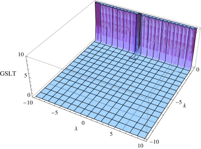
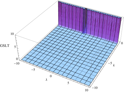
The higher powers of curvature can be made available for larger values of kπ‘˜k and one can examine the validity of GSLT. If one consider the dust case Ο‰=0πœ”0\omega=0, then the possible role of Ξ»πœ†\lambda and kπ‘˜k can be seen from graphical description as shown in Figure 1.
Refer to caption
Refer to caption
Figure 1: Evolution of GSLT for different values of parameters kπ‘˜k and Ξ»πœ†\lambda (a) for present epoch z=0𝑧0z=0 and (b) for z=βˆ’0.9𝑧0.9z=-0.9

In the second case, the GSLT for the f​(R,T)=R+2​f​(T)𝑓𝑅𝑇𝑅2𝑓𝑇f(R,T)=R+2f(T) model demands the following inequality to be fulfilled

Th​S^Λ™=HΛ™22​H4​G^β©Ύ0,w​h​e​r​eG^=G+2​f​(T)/8​π.formulae-sequencesubscriptπ‘‡β„ŽΛ™^𝑆superscript˙𝐻22superscript𝐻4^𝐺0π‘€β„Žπ‘’π‘Ÿπ‘’^𝐺𝐺2𝑓𝑇8πœ‹T_{h}\dot{\hat{S}}=\frac{\dot{H}^{2}}{2H^{4}\hat{G}}\geqslant 0,\quad where\quad\hat{G}=G+2f(T)/8{\pi}.

Here we consider the power law solution of the form f​(T)=a1​T+a2​Tk𝑓𝑇subscriptπ‘Ž1𝑇subscriptπ‘Ž2superscriptπ‘‡π‘˜f(T)=a_{1}T+a_{2}T^{k}, where a1subscriptπ‘Ž1a_{1} and a2subscriptπ‘Ž2a_{2} are parameters. Following [13] for the dust case, we set a1=1subscriptπ‘Ž11a_{1}=1 and a2=23βˆ’2​k​3kβˆ’1​k3βˆ’2​k4+2​ksubscriptπ‘Ž2superscript232π‘˜superscript3π‘˜1superscriptπ‘˜32π‘˜42π‘˜a_{2}=\frac{2^{3-2k}3^{k-1}k^{3-2k}}{4+2k}. Thus the above inequality takes the form

Th​S^Λ™=9​π​(4+2​k)k2​[(4+2​k)​(8​π​G+1)+23βˆ’2​k​3kβˆ’1​k4βˆ’2​k​Tkβˆ’1]β©Ύ0.subscriptπ‘‡β„ŽΛ™^𝑆9πœ‹42π‘˜superscriptπ‘˜2delimited-[]42π‘˜8πœ‹πΊ1superscript232π‘˜superscript3π‘˜1superscriptπ‘˜42π‘˜superscriptπ‘‡π‘˜10T_{h}\dot{\hat{S}}=\frac{9\pi(4+2k)}{k^{2}[(4+2k)(8\pi{G}+1)+2^{3-2k}3^{k-1}k^{4-2k}T^{k-1}]}\geqslant 0.

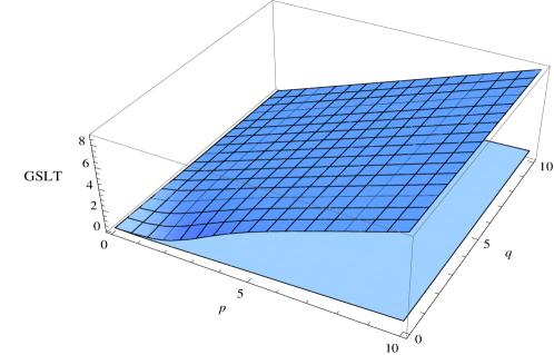
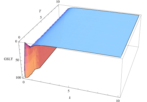
This shows that the GSLT holds for the f​(T)𝑓𝑇f(T) power law model and its validity is shown in Figure 2.
Refer to caption
Figure 2: Evolution of GSLT for case (ii) versus T𝑇T and kπ‘˜k.

3.2 f​(R,T)=f1​(R)+f2​(R)​f3​(T)𝑓𝑅𝑇subscript𝑓1𝑅subscript𝑓2𝑅subscript𝑓3𝑇f(R,T)=f_{1}(R)+f_{2}(R)f_{3}(T)

A more general f​(R,T)𝑓𝑅𝑇f(R,T) gravity model is of the form [12]

f​(R,T)=f1​(R)+f2​(R)​f3​(T),𝑓𝑅𝑇subscript𝑓1𝑅subscript𝑓2𝑅subscript𝑓3𝑇f(R,T)=f_{1}(R)+f_{2}(R)f_{3}(T), (25)

where fi​(i=1,2)subscript𝑓𝑖𝑖12f_{i}~{}(i=1,2) are functions of R𝑅R and f3subscript𝑓3f_{3} is function of T𝑇T. For a dust matter source, the field equation is obtained as

Rα​β​[f1​R+f2​R​f3]βˆ’12​gα​β​f1+(gΞ±β€‹Ξ²β€‹β–‘βˆ’βˆ‡Ξ±βˆ‡Ξ²)​[f1​R+f2​R​f3]subscript𝑅𝛼𝛽delimited-[]subscript𝑓1𝑅subscript𝑓2𝑅subscript𝑓312subscript𝑔𝛼𝛽subscript𝑓1subscript𝑔𝛼𝛽░subscriptβˆ‡π›Όsubscriptβˆ‡π›½delimited-[]subscript𝑓1𝑅subscript𝑓2𝑅subscript𝑓3\displaystyle R_{\alpha\beta}[f_{1R}+f_{2R}f_{3}]-\frac{1}{2}g_{\alpha\beta}f_{1}+(g_{\alpha\beta}{\Box}-{\nabla}_{\alpha}{\nabla}_{\beta})[f_{1R}+f_{2R}f_{3}] (26)
=\displaystyle= 8​π​G​Tα​β(m)+Tα​β(m)​f2​f3​T+12​gα​β​f2​f3.8πœ‹πΊsuperscriptsubscriptπ‘‡π›Όπ›½π‘šsuperscriptsubscriptπ‘‡π›Όπ›½π‘šsubscript𝑓2subscript𝑓3𝑇12subscript𝑔𝛼𝛽subscript𝑓2subscript𝑓3\displaystyle 8{\pi}GT_{\alpha\beta}^{(m)}+T_{\alpha\beta}^{(m)}f_{2}f_{3T}+\frac{1}{2}g_{\alpha\beta}f_{2}f_{3}.

An equivalent Einstein field equation can be obtained with GE​f​f=1f1​R+f2​R​f3​(G+f2​f3​T8​π)subscript𝐺𝐸𝑓𝑓1subscript𝑓1𝑅subscript𝑓2𝑅subscript𝑓3𝐺subscript𝑓2subscript𝑓3𝑇8πœ‹G_{Eff}=\frac{1}{f_{1R}+f_{2R}f_{3}}\left(G+\frac{f_{2}f_{3T}}{8\pi}\right), whereas

T^α​β(d​c)=1f1​R+f2​R​f3[12gα​β(f1+f2f3)βˆ’R(f1​R+f2​Rf3))+(βˆ‡Ξ±βˆ‡Ξ²\displaystyle\hat{T}_{\alpha\beta}^{(dc)}=\frac{1}{f_{1R}+f_{2R}f_{3}}\left[\frac{1}{2}g_{\alpha\beta}(f_{1}+f_{2}f_{3})-R(f_{1R}+f_{2R}f_{3}))+({\nabla}_{\alpha}{\nabla}_{\beta}\right. (27)
βˆ’\displaystyle- gα​β░)(f1​R+f2​Rf3)].\displaystyle\left.g_{\alpha\beta}{\Box})(f_{1R}+f_{2R}f_{3})\right].

In the following discussion, we define π’₯​(R,T)=f1​R​(R)+f2​R​(R)​f3​(T)π’₯𝑅𝑇subscript𝑓1𝑅𝑅subscript𝑓2𝑅𝑅subscript𝑓3𝑇\mathcal{J}(R,T)=f_{1R}(R)+f_{2R}(R)f_{3}(T).

For this f​(R,T)𝑓𝑅𝑇f(R,T) model, the field equation are identical to Eqs.(9)-(10), whereas

ρ^d​csubscript^πœŒπ‘‘π‘\displaystyle\hat{\rho}_{dc} =\displaystyle= 18​π​G​ℬ​[12​(R​π’₯βˆ’f1βˆ’f2​f3)βˆ’n​H​(R˙​π’₯R+T˙​π’₯T)],18πœ‹πΊβ„¬delimited-[]12𝑅π’₯subscript𝑓1subscript𝑓2subscript𝑓3𝑛𝐻˙𝑅subscriptπ’₯𝑅˙𝑇subscriptπ’₯𝑇\displaystyle\frac{1}{8{\pi}G\mathcal{B}}\left[\frac{1}{2}(R\mathcal{J}-f_{1}-f_{2}f_{3})-nH(\dot{R}\mathcal{J}_{R}+\dot{T}\mathcal{J}_{T})\right], (28)
p^d​csubscript^𝑝𝑑𝑐\displaystyle{\hat{p}}_{dc} =\displaystyle= 18​π​G​ℬ[βˆ’12(Rπ’₯βˆ’f1βˆ’f2f3)+(nβˆ’1)H(RΛ™π’₯R+TΛ™π’₯T)+RΒ¨π’₯R\displaystyle\frac{1}{8{\pi}G\mathcal{B}}\left[-\frac{1}{2}(R\mathcal{J}-f_{1}-f_{2}f_{3})+(n-1)H(\dot{R}\mathcal{J}_{R}+\dot{T}\mathcal{J}_{T})+\ddot{R}\mathcal{J}_{R}\right. (29)
+\displaystyle+ RΛ™2π’₯R​R+2RΛ™TΛ™π’₯R​T+TΒ¨π’₯T+TΛ™2π’₯T​T]\displaystyle\left.\dot{R}^{2}\mathcal{J}_{RR}+2\dot{R}\dot{T}\mathcal{J}_{RT}+\ddot{T}\mathcal{J}_{T}+\dot{T}^{2}\mathcal{J}_{TT}\right]

and ℬ​(R,T)=(1+f2​(R)​f3​T​(T)8​π​G)ℬ𝑅𝑇1subscript𝑓2𝑅subscript𝑓3𝑇𝑇8πœ‹πΊ\mathcal{B}(R,T)=\left(1+\frac{f_{2}(R)f_{3T}(T)}{8{\pi}G}\right) which includes contributions from both matter and geometry. The total energy exchange term for this model is given by

qt=n​(nβˆ’1)16​π​G​(H2+ka2)β€‹βˆ‚t(π’₯ℬ).subscriptπ‘žπ‘‘π‘›π‘›116πœ‹πΊsuperscript𝐻2π‘˜superscriptπ‘Ž2subscript𝑑π’₯ℬq_{t}=\frac{n(n-1)}{16{\pi}G}(H^{2}+\frac{k}{a^{2}})\partial_{t}\left(\frac{\mathcal{J}}{\mathcal{B}}\right). (30)

Now we analyze the validity of the FLT and GSLT for the above model.

3.2.1 First Law of Thermodynamics

The Wald entropy S^h=A/4​GE​f​fsubscript^π‘†β„Žπ΄4subscript𝐺𝐸𝑓𝑓\hat{S}_{h}=A/4G_{Eff} for function (25) becomes

S^h=n​Ω^n​r~Anβˆ’1​π’₯4​G​ℬ.subscript^π‘†β„Žπ‘›subscript^Ω𝑛superscriptsubscript~π‘Ÿπ΄π‘›1π’₯4𝐺ℬ\hat{S}_{h}=\frac{n\hat{\Omega}_{n}\tilde{r}_{A}^{n-1}\mathcal{J}}{4G\mathcal{B}}. (31)

In this case, FLT involves the energy flux δ​Q𝛿𝑄\delta{Q} and entropy production terms of the form [34]

δ​Q𝛿𝑄\displaystyle\delta{Q} =\displaystyle= βˆ’d​E^+n2​Ωn​r~Anβˆ’1​(ρt​o​tβˆ’pt​o​t)​d​r~A+n​(nβˆ’1)16​π​G​Ωn​r~Anβˆ’2​d​(π’₯ℬ)𝑑^𝐸𝑛2subscriptΩ𝑛superscriptsubscript~π‘Ÿπ΄π‘›1subscriptπœŒπ‘‘π‘œπ‘‘subscriptπ‘π‘‘π‘œπ‘‘π‘‘subscript~π‘Ÿπ΄π‘›π‘›116πœ‹πΊsubscriptΩ𝑛subscriptsuperscript~π‘Ÿπ‘›2𝐴𝑑π’₯ℬ\displaystyle-d\hat{E}+\frac{n}{2}\Omega_{n}\tilde{r}_{A}^{n-1}(\rho_{tot}-p_{tot})d\tilde{r}_{A}+\frac{n(n-1)}{16{\pi}G}\Omega_{n}\tilde{r}^{n-2}_{A}d\left(\frac{\mathcal{J}}{\mathcal{B}}\right) (32)
=\displaystyle= βˆ’d​E^+Wt​o​t​d​𝕍+𝕍​qt​o​t​d​t+Th​S^h​d​(π’₯ℬ).𝑑^𝐸subscriptπ‘Šπ‘‘π‘œπ‘‘π‘‘π•π•subscriptπ‘žπ‘‘π‘œπ‘‘π‘‘π‘‘subscriptπ‘‡β„Žsubscript^π‘†β„Žπ‘‘π’₯ℬ\displaystyle-d\hat{E}+W_{tot}d\mathbb{V}+\mathbb{V}q_{tot}dt+T_{h}\hat{S}_{h}d\left(\frac{\mathcal{J}}{\mathcal{B}}\right).
dȷ​S^hsubscript𝑑italic-Θ·subscript^π‘†β„Ž\displaystyle d_{\jmath}\hat{S}_{h} =\displaystyle= βˆ’1Th​𝕍​qt​o​t​d​tβˆ’Sh​d​(π’₯ℬ)1subscriptπ‘‡β„Žπ•subscriptπ‘žπ‘‘π‘œπ‘‘π‘‘π‘‘subscriptπ‘†β„Žπ‘‘π’₯ℬ\displaystyle-\frac{1}{T_{h}}\mathbb{V}q_{tot}dt-S_{h}d\left(\frac{\mathcal{J}}{\mathcal{B}}\right) (33)
=\displaystyle= βˆ’n​Ωn​(H2+ka2)nβˆ’12​((n+1)​H2+HΛ™+n​ka2)​d​(π’₯/ℬ)4​G​(2​H2+HΛ™+ka2).𝑛subscriptΩ𝑛superscriptsuperscript𝐻2π‘˜superscriptπ‘Ž2𝑛12𝑛1superscript𝐻2Λ™π»π‘›π‘˜superscriptπ‘Ž2𝑑π’₯ℬ4𝐺2superscript𝐻2Λ™π»π‘˜superscriptπ‘Ž2\displaystyle-\frac{n\Omega_{n}(H^{2}+\frac{k}{a^{2}})^{\frac{n-1}{2}}((n+1)H^{2}+\dot{H}+n\frac{k}{a^{2}})d(\mathcal{J}/\mathcal{B})}{4G(2H^{2}+\dot{H}+\frac{k}{a^{2}})}.

The f​(R,T)𝑓𝑅𝑇f(R,T) gravity model, f​(R,T)=f1​(R)+f2​(R)​f3​(T)𝑓𝑅𝑇subscript𝑓1𝑅subscript𝑓2𝑅subscript𝑓3𝑇f(R,T)=f_{1}(R)+f_{2}(R)f_{3}(T) involves the explicit non-minimal gravitational coupling between matter and curvature. Results obtained using this theory would be different from other models such as f​(R)𝑓𝑅f(R) theory. The coupling of matter and geometry reveals that the matter energy-momentum tensor is no longer conserved and there is an energy transfer between the two components. Due to this interaction, the energy exchange term qtsubscriptπ‘žπ‘‘q_{t} is found to be non-zero, so the entropy production term would be an additional term in this modified gravity. Hence, the FLT is established in more general f​(R,T)𝑓𝑅𝑇f(R,T) gravity and entropy production is induced in a non-equilibrium treatment of thermodynamics [21, 34]. In recent papers [33], Bamba et al. shown that the entropy production term can be incorporated by redefinition of the field equations. However, in this theory, such treatment is not useful as shown in [34].

3.2.2 Generalized Second Law of Thermodynamics

To develop the GSLT for the second model, we consider the Gibbs equation (18). The horizon entropy is determined from FLT. The necessary constraint for the validity of the GSLT is shown in Eq.(19). For the f​(R,T)𝑓𝑅𝑇f(R,T) model (25), we obtain

n​(nβˆ’1)​Ω^n16​π​H​G[2Hr~Λ™A[(bβˆ’1)+r~Λ™Ar~Anβˆ’4(2βˆ’b)](π’₯ℬ)+(1βˆ’b)Hr~A\displaystyle\frac{n(n-1)\hat{\Omega}_{n}}{16{\pi}HG}\left[2H\dot{\tilde{r}}_{A}\left[(b-1)+\dot{\tilde{r}}_{A}\tilde{r}_{A}^{n-4}(2-b)\right]\left(\frac{\mathcal{J}}{\mathcal{B}}\right)+(1-b)H\tilde{r}_{A}\right. (34)
Γ—\displaystyle\times βˆ‚t(π’₯ℬ)]β©Ύ0,wherer~Λ™A=βˆ’r~βˆ’3AH(HΛ™βˆ’ΞΊa2).\displaystyle\left.\partial_{t}\left(\frac{\mathcal{J}}{\mathcal{B}}\right)\right]\geqslant 0,\quad where\quad\quad\dot{\tilde{r}}_{A}=-\tilde{r}^{-3}_{A}H(\dot{H}-\frac{\kappa}{a^{2}}).

The effective gravitational coupling constant for this model is GE​f​f=G​ℬ/π’₯subscript𝐺𝐸𝑓𝑓𝐺ℬπ’₯G_{Eff}=G\mathcal{B}/\mathcal{J}. We can impose the condition ℬ/π’₯>0ℬπ’₯0\mathcal{B}/\mathcal{J}>0 to keep GE​f​f>0subscript𝐺𝐸𝑓𝑓0G_{Eff}>0. For the positive temperature condition (HΛ™βˆ’ka2)>βˆ’2​(H2+ka2)Λ™π»π‘˜superscriptπ‘Ž22superscript𝐻2π‘˜superscriptπ‘Ž2(\dot{H}-\frac{k}{a^{2}})>-2(H^{2}+\frac{k}{a^{2}}) with b<1𝑏1b<1, Eq.(34) is reduced to

n​(nβˆ’1)​Ω^n​(H2+ka2)βˆ’n2+116​π​G​ℬ​[4​H​π’₯+(1βˆ’b)β€‹β„¬β€‹βˆ‚t(π’₯ℬ)]β©Ύ0.𝑛𝑛1subscript^Ω𝑛superscriptsuperscript𝐻2π‘˜superscriptπ‘Ž2𝑛2116πœ‹πΊβ„¬delimited-[]4𝐻π’₯1𝑏ℬsubscript𝑑π’₯ℬ0\displaystyle\frac{n(n-1)\hat{\Omega}_{n}(H^{2}+\frac{k}{a^{2}})^{-\frac{n}{2}+1}}{16{\pi}G\mathcal{B}}\left[4H\mathcal{J}+(1-b){\mathcal{B}}\partial_{t}\left(\frac{\mathcal{J}}{\mathcal{B}}\right)\right]\geqslant 0. (35)

This shows that the GSLT is valid only if βˆ‚t(π’₯/ℬ)>0subscript𝑑π’₯ℬ0\partial_{t}(\mathcal{J}/\mathcal{B})>0. If the gravitational coupling constant is indeed a constant, the GSLT is always protected. If βˆ‚t(π’₯/ℬ)<0subscript𝑑π’₯ℬ0\partial_{t}(\mathcal{J}/\mathcal{B})<0, then the GSLT can hold only if βˆ£βˆ‚t(π’₯/ℬ)π’₯/β„¬βˆ£β©½4​H1βˆ’bdelimited-∣∣subscript𝑑π’₯ℬπ’₯ℬ4𝐻1𝑏\mid\frac{\partial_{t}(\mathcal{J}/\mathcal{B})}{\mathcal{J}/\mathcal{B}}\mid\leqslant\frac{4H}{1-b}. The GSLT in f​(R)𝑓𝑅f(R) theory can be retrieved for f3​(T)=0subscript𝑓3𝑇0f_{3}(T)=0. If Tt∼Th∼subscript𝑇𝑑subscriptπ‘‡β„ŽT_{t}\thicksim{T}_{h}, then the condition (35) becomes

n​(nβˆ’1)​Ω^n​(H2+ka2)βˆ’(n2+1)16​π​G​ℬ​[H​(HΛ™βˆ’ka2)2​π’₯]β©Ύ0.𝑛𝑛1subscript^Ω𝑛superscriptsuperscript𝐻2π‘˜superscriptπ‘Ž2𝑛2116πœ‹πΊβ„¬delimited-[]𝐻superscriptΛ™π»π‘˜superscriptπ‘Ž22π’₯0\displaystyle\frac{n(n-1)\hat{\Omega}_{n}(H^{2}+\frac{k}{a^{2}})^{-(\frac{n}{2}+1)}}{16{\pi}G\mathcal{B}}\left[H(\dot{H}-\frac{k}{a^{2}})^{2}\mathcal{J}\right]\geqslant 0.
Refer to caption
Figure 3: Evolution of GSLT for the model (36) with m=2π‘š2m=2. The curve with larger slope corresponds to z=βˆ’0.9𝑧0.9z=-0.9 while the other represents the present value (z=0𝑧0z=0).
Refer to caption
Refer to caption
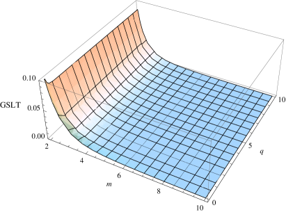
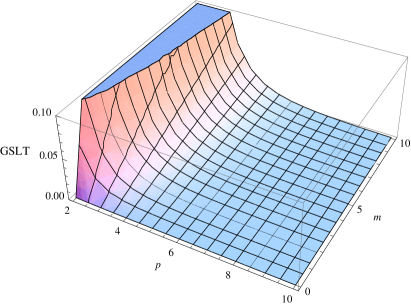
Figure 4: One can choose the specific value of one parameter and vary the others. In left panel, we choose p=1𝑝1p=1 and show the constraints on parameters mπ‘šm and qπ‘žq. The right panel represents the parametric values of mπ‘šm and p𝑝p for fixed q=1π‘ž1q=1.

We consider the f​(R,T)𝑓𝑅𝑇f(R,T) model (25) with f1​(R)=R,f2​(R)=Rpformulae-sequencesubscript𝑓1𝑅𝑅subscript𝑓2𝑅superscript𝑅𝑝f_{1}(R)=R,~{}f_{2}(R)=R^{p} and f3​(R)=Tq,(p,q>0)subscript𝑓3𝑅superscriptπ‘‡π‘žπ‘π‘ž0f_{3}(R)=T^{q},~{}(p,q>0) so that in 4-dimensional flat FRW metric, the GSLT becomes

Th​S^Λ™=HΛ™2​(1+p​Rpβˆ’1​Tq)2​H4​G​(1+Rp​Tq8​π​G)β©Ύ0.subscriptπ‘‡β„ŽΛ™^𝑆superscript˙𝐻21𝑝superscript𝑅𝑝1superscriptπ‘‡π‘ž2superscript𝐻4𝐺1superscript𝑅𝑝superscriptπ‘‡π‘ž8πœ‹πΊ0\displaystyle T_{h}\dot{\hat{S}}=\frac{\dot{H}^{2}(1+pR^{p-1}T^{q})}{2H^{4}G\left(1+\frac{R^{p}T^{q}}{8\pi{G}}\right)}\geqslant 0. (36)

For the power law case a​(t)=a0​tmπ‘Žπ‘‘subscriptπ‘Ž0superscriptπ‘‘π‘ša(t)=a_{0}t^{m} with ρ=ρ0​aβˆ’3𝜌subscript𝜌0superscriptπ‘Ž3\rho=\rho_{0}a^{-3}, this can be written as

Th​S^Λ™=8Ο€[1+p(6m(2mβˆ’1)tβˆ’2]pβˆ’1(ρ0tβˆ’3​m)q2​m2​[8​π​G+(6​m​(2​mβˆ’1)​tβˆ’2)pβˆ’1​(ρ0​tβˆ’3​m)q]β©Ύ0.\displaystyle T_{h}\dot{\hat{S}}=\frac{8\pi[1+p(6m(2m-1)t^{-2}]^{p-1}(\rho_{0}t^{-3m})^{q}}{2m^{2}[8\pi{G}+(6m(2m-1)t^{-2})^{p-1}(\rho_{0}t^{-3m})^{q}]}\geqslant 0. (37)

We have examined the validity of relation (37) and developed constraints on the parameters mπ‘šm, p𝑝p and qπ‘žq. The results are shown in Figures 3 and 4.

4 Conclusions

In this paper, the thermodynamics properties have been discussed in more general f​(R,T)𝑓𝑅𝑇f(R,T) theory. The non-equilibrium treatment of thermodynamics is addressed for two particular models of f​(R,T)𝑓𝑅𝑇f(R,T) gravity. In this modified theory, accelerated expansion may produce not just from scalar curvature part to the entire energy density of universe, but may include a matter component as well. The consequences of f​(R,T)𝑓𝑅𝑇f(R,T) theory may contribute to significant results when compared to other modified gravitational theories, applicable to various problems of contemporary interest such as accelerated cosmic expansion, gravitational collapse, dark matter and the detection of gravitational waves [40]. The detection of gravitational waves could be an excellent way to test general relativity and modified theories of gravity. Corda [40] has investigated the detection of gravitational waves in f​(R)𝑓𝑅f(R) theory and it would be appealing to explore this issue in f​(R,T)𝑓𝑅𝑇f(R,T) theory.

It is shown that representation of equilibrium thermodynamics is not executable in this theory [34]. Hence the non-equilibrium treatment of thermodynamics is employed to discuss the laws of thermodynamics. Here, we studied two particular models of f​(R,T)𝑓𝑅𝑇f(R,T) theory to show the consequences of explicit coupling of matter and geometry. The gravitational coupling between matter and higher derivatives terms of curvature describes a transfer of energy and momentum beyond that normally existing in curved spaces. This interaction leads to the entropy production term in this modified gravity. The FLT is formulated by employing the Wald’s entropy relation. We remark that an entropy production term is produced in this work but no such term in present in GR, Gauss-Bonnet [22], Lovelock [22] and braneworld [24] theories of gravity.

The validity of GSLT has also been investigated in this work. We have found that the GSLT holds with the conditions namely, attractive nature of gravity and temperature being positive. In fact, it is natural to assume the relation Tt=b​Thsubscript𝑇𝑑𝑏subscriptπ‘‡β„ŽT_{t}=bT_{h} and proportionality constant b𝑏b can be considered as unity, implying that the system is in thermal-equilibrium. Generally, the horizon temperature cannot match the temperature of all energy sources within the horizon, and the two mechanisms must experience interaction for some interval of time ahead of achieving the thermal-equilibrium. Moreover, the gravitational curvature-matter coupling in f​(R,T)𝑓𝑅𝑇f(R,T) theory may produce the unscripted flow of energy between the horizon and fluid. Also, the energy fluid of dark components does not permit the effective gravitational constant to be an approximate constant. In the limiting choice of thermal-equilibrium, we assume that Ttsubscript𝑇𝑑T_{t} is very close to Thsubscriptπ‘‡β„ŽT_{h}. We find that the GSLT is fulfilled in both phantom and quintessence regimes of the universe which seems to be consistent with refs.[41]. Furthermore, we have also developed constraints on some concrete f​(R,T)𝑓𝑅𝑇f(R,T) models corresponding to power law solution. It is significant to remark that the equilibrium treatment of thermodynamics in f​(R,T)𝑓𝑅𝑇f(R,T) theory would benefit from further study.

Acknowledgment

The authors would like to thank the Higher Education Commission, Islamabad, Pakistan for its financial support through the Indigenous Ph.D. 5000 Fellowship Program Batch-VII.

References

  • [1] S. Perlmutter et al.: Astrophys. J. 517, 565(1999).
  • [2] D. N. Spergel et al.: Astrophys. J. Suppl. 170, 377(2007).
  • [3] M. Tegmark et al.: Phys. Rev. D 69, 103501(2004).
  • [4] D. J. Eisentein et al.: Astrophys. J. 633, 560(2005).
  • [5] B. Jain, A. Taylor: Phys. Rev. Lett. 91, 141302(2003).
  • [6] M. Sharif, M. Zubair: Int. J. Mod. Phys. D 19, 1957(2010).
  • [7] M. Sharif, M. Zubair: Astrophys. Space Sci. 330, 399(2010); ibid. 339, 45(2012)
  • [8] Li, M., Li, X.-D., Wang, S. and Wang, Y.: Commun. Theor. Phys. 56, 525(2011).
  • [9] A. De Felice, S. Tsujikawa: Living Rev. Rel. 13, 3(2010).
  • [10] R. Ferraro, F. Fiorini: Phys. Rev. D 75, 084031(2007).
  • [11] G. R. Bengochea, R. Ferraro: Phys. Rev. D 79, 124019(2009).
  • [12] T. Harko, F. S. N. Lobo, S. Nojiri, S. D. Odintsov: Phys. Rev. D 84, 024020(2011).
  • [13] M. Sharif, and M. Zubair: J. Phys. Soc. Jpn. 81, 114005(2012); ibid. 82, 014002(2013).
  • [14] K. Bamba, S. Capozziello, S. Nojiri, S. D. Odintsov: Astrophys. Space Sci. 345, 155(2012).
  • [15] J. M. Bardeen, B. Carter, S. W. Hawking: Commun. Math. Phys. 31, 161(1973).
  • [16] S. W. Hawking: Commun. Math. Phys. 43, 199(1975).
  • [17] J. D. Bekenstein: Phys. Rev. D 7, 2333(1973).
  • [18] T. Jacobson: Phys. Rev. Lett. 75, 1260(1995).
  • [19] T. Padmanabhan: Phys. Rep. 406, 49(2005).
  • [20] R. G. Cai, S. P. Kim: JHEP 02, 050(2005).
  • [21] C. Eling, R. Guedens, T. Jacobson: Phys. Rev. Lett. 96, 121301(2006).
  • [22] M. Akbar, R. G. Cai: Phys. Rev. D 75, 084003(2007).
  • [23] S. A. Hayward: S. Mukohyama, M. Ashworth, Phys. Lett. A 256, 347(1999).
  • [24] A. Sheykhi, B. Wang, R. G. Cai: Phys. Rev. D 76, 023515(2007).
  • [25] M. Akbar, R. G. Cai: Phys. Lett. B 648, 243(2007).
  • [26] R. G. Cai, L. M. Cao: Phys. Rev. D 75 064008(2007).
  • [27] S.-F. Wu, B. Wang, G.-H. Yang, P.-M. Zhang: Class. Quantum Grav. 25, 235018(2008).
  • [28] Y. Gong, A. Wang: Phys. Rev. Lett. 99, 211301(2007).
  • [29] C. Eling: JHEP 11, 048(2008).
  • [30] E. Elizalde, P. J. Silva: Phys. Rev. D 78, 061501(2008).
  • [31] S.-F. Wu, X.-H. Ge, P.-M. Zhang, G.-H. Yang: Phys. Rev. D 81, 044034(2010).
  • [32] K. Bamba, C. Q. Geng: Phys. Lett. B 679, 282(2009).
  • [33] K. Bamba, C. Q. Geng: JCAP 06, 014(2010); ibid. 11, 008(2011).
  • [34] M. Sharif, M. Zubair: JCAP 03, 028(2012); ibid. 05, E01(2012).
  • [35] L. D. Landau, E. M. Lifshitz: The Classical Theory of Fileds (Butterworth-Heinemann, 2002).
  • [36] R. M. Wald: Phys. Rev. D 48, 3427(1993).
  • [37] R. Brustein, D. Gorbonos, M. Hadad: Phys. Rev. D 79, 044025(2009).
  • [38] C. W. Misner, D. H. Sharp: Phys. Rev. 136, B571(1964).
  • [39] G. Izquierdo, D. Pavon: Phys. Lett. B 633, 420(2006).
  • [40] C. Corda: Eur. Phys. J. C 65, 257(2010).
  • [41] S. Nojiri, S. D. Odintsov: Phys. Rev. D 72, 023003(2005).