11institutetext: G. K. Befekadu  (🖂) 22institutetext: Department of Electrical Engineering, University of Notre Dame, Notre Dame, IN 46556, USA.
Tel.: +1 574 631 6618
Fax: +1 574 631 4393
22email: gbefekadu1@nd.edu
33institutetext: P. J. Antsaklis 44institutetext: Department of Electrical Engineering, University of Notre Dame, Notre Dame, IN 46556, USA.
44email: antsaklis.1@nd.edu

On the risk-sensitive escape control for diffusion processes pertaining to an expanding construction of distributed control systems

Getachew K. Befekadu    Panos J. Antsaklis
(Received: September 21, 2014 / Accepted: date)
Abstract

In this paper, we consider an expanding construction of a distributed control system, which is obtained by adding a new subsystem one after the other, until all n𝑛n subsystems, where n2𝑛2n\geq 2, are included in the distributed control system. It is assumed that a small random perturbation enters only into the first subsystem and is then subsequently transmitted to the other subsystems. Moreover, for any {2,,n}2𝑛\ell\in\{2,\ldots,n\}, the distributed control system, compatible with the expanding construction, which is obtained from the first \ell subsystems, satisfies an appropriate Hörmander condition. As a result of this, the diffusion process is degenerate, i.e., the backward operator associated with it is a degenerate parabolic equation. Our main interest here is to prevent the diffusion process (that corresponds to a particular subsystem) from leaving a given bounded open domain. In particular, we consider a risk-sensitive version of the mean escape time criterion with respect to each of the subsystems. Using a variational representation, we characterize the risk-sensitive escape control for the diffusion process as the lower and upper values of an associated stochastic differential game. Finally, we comment on the implication of our results, where one is also interested in evaluating the performance of the risk-sensitive escape control, when there is some modeling error in the distributed control system.

Keywords:
Diffusion processes distributed control systems exit probabilities risk-sensitive escape control
journal:

1 Introduction

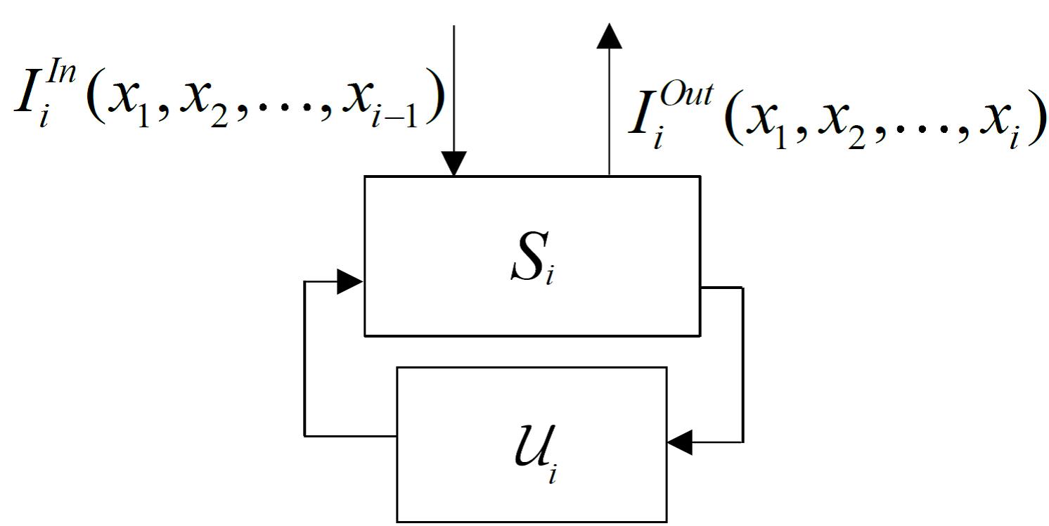
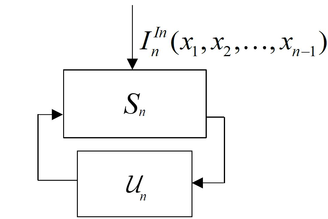
We consider the diffusion processes (x1(t),x2(t),,xn(t))superscript𝑥1𝑡superscript𝑥2𝑡superscript𝑥𝑛𝑡\bigl{(}x^{1}(t),x^{2}(t),\ldots,x^{n}(t)\bigr{)} pertaining to the following distributed control system, with small random perturbations (see Fig. 1b)111This work is, in some sense, a continuation of our previous paper BefAn14 .

dx1(t)=m1(x1(t),u1(t))dt+ϵσ(x1(t))dW(t)dx2(t)=m2(x1(t),x2(t),u2(t))dtdxn(t)=mn(x1(t),x2(t),,xn(t),un(t))dtx1(0)=x01,x2(0)=x02,,xn(0)=x0n,t0,n2}cases𝑑superscript𝑥1𝑡subscript𝑚1superscript𝑥1𝑡subscript𝑢1𝑡𝑑𝑡italic-ϵ𝜎superscript𝑥1𝑡𝑑𝑊𝑡𝑑superscript𝑥2𝑡subscript𝑚2superscript𝑥1𝑡superscript𝑥2𝑡subscript𝑢2𝑡𝑑𝑡𝑑superscript𝑥𝑛𝑡subscript𝑚𝑛superscript𝑥1𝑡superscript𝑥2𝑡superscript𝑥𝑛𝑡subscript𝑢𝑛𝑡𝑑𝑡formulae-sequencesuperscript𝑥10superscriptsubscript𝑥01formulae-sequencesuperscript𝑥20superscriptsubscript𝑥02formulae-sequencesuperscript𝑥𝑛0superscriptsubscript𝑥0𝑛formulae-sequence𝑡0𝑛2\displaystyle\left.\begin{array}[]{l}dx^{1}(t)=m_{1}\bigl{(}x^{1}(t),u_{1}(t)\bigr{)}dt+\sqrt{\epsilon}\sigma\bigl{(}x^{1}(t)\bigr{)}dW(t)\\ dx^{2}(t)=m_{2}\bigl{(}x^{1}(t),x^{2}(t),u_{2}(t)\bigr{)}dt\\ \quad\quad\quad~{}\vdots\\ dx^{n}(t)=m_{n}\bigl{(}x^{1}(t),x^{2}(t),\ldots,x^{n}(t),u_{n}(t)\bigr{)}dt\\ x^{1}(0)=x_{0}^{1},\,\,x^{2}(0)=x_{0}^{2},\,\,\ldots,\,\,x^{n}(0)=x_{0}^{n},\,\,t\geq 0,\,\,n\geq 2\end{array}\right\} (6)

where

  • -

    xi()superscript𝑥𝑖x^{i}(\cdot) is an dsuperscript𝑑\mathbb{R}^{d}-valued diffusion process that corresponds to the i𝑖ith-subsystem (with i{1,2,,n}𝑖12𝑛i\in\{1,2,\ldots,n\}),

  • -

    the functions mi:d×d××ditimes×𝒰id:subscript𝑚𝑖subscriptsuperscript𝑑superscript𝑑superscript𝑑𝑖timessubscript𝒰𝑖superscript𝑑m_{i}\colon\underbrace{\mathbb{R}^{d}\times\mathbb{R}^{d}\times\cdots\times\mathbb{R}^{d}}_{i-\rm{times}}\times\,\mathcal{U}_{i}\rightarrow\mathbb{R}^{d} are uniformly Lipschitz, with bounded first derivatives, ϵitalic-ϵ\epsilon is a small positive number (which is related to the random perturbation level in the system),

  • -

    σ:dd×m:𝜎superscript𝑑superscript𝑑𝑚\sigma\colon\mathbb{R}^{d}\rightarrow\mathbb{R}^{d\times m} is Lipschitz with the least eigenvalue of σ()σT()𝜎superscript𝜎𝑇\sigma(\cdot)\,\sigma^{T}(\cdot) uniformly bounded away from zero, i.e.,

    σ(x)σT(x)λId×d,xd,formulae-sequence𝜎𝑥superscript𝜎𝑇𝑥𝜆subscript𝐼𝑑𝑑for-all𝑥superscript𝑑\displaystyle\sigma(x)\,\sigma^{T}(x)\geq\lambda I_{d\times d},\quad\forall x\in\mathbb{R}^{d},

    for some λ>0𝜆0\lambda>0,

  • -

    W()𝑊W(\cdot) (with W(0)=0𝑊00W(0)=0) is a m𝑚m-dimensional standard Wiener process,

  • -

    ui()subscript𝑢𝑖u_{i}(\cdot) is a 𝒰isubscript𝒰𝑖\,\mathcal{U}_{i}-valued measurable control process to the i𝑖ith-subsystem, i.e., an admissible control from the measurable set  𝒰irisubscript𝒰𝑖superscriptsubscript𝑟𝑖\mathcal{U}_{i}\subset\mathbb{R}^{r_{i}}.

In this paper, we identify two admissible controls ui,u~i𝒰isubscript𝑢𝑖subscript~𝑢𝑖subscript𝒰𝑖u_{i},\,\tilde{u}_{i}\in\mathcal{U}_{i}, for i=1,2,n𝑖12𝑛i=1,2\ldots,n, being the same on [0,s]0𝑠[0,\,s] if Prob{ui(t)=u~i(t),t[0,s]}=1Probsubscript𝑢𝑖𝑡subscript~𝑢𝑖𝑡for-all𝑡0𝑠1\operatorname{Prob}\bigl{\{}u_{i}(t)=\tilde{u}_{i}(t),\,\forall t\in[0,\,s]\bigr{\}}=1. If ui𝒰isubscript𝑢𝑖subscript𝒰𝑖u_{i}\in\mathcal{U}_{i}, then, for every s[0,)𝑠0s\in[0,\,\infty), there exists a Borel measurable function γis:𝒞([0,T],m)𝒰i:superscriptsubscript𝛾𝑖𝑠𝒞0𝑇superscript𝑚subscript𝒰𝑖\gamma_{i}^{s}\colon\mathscr{C}\bigl{(}[0,\,T],\mathbb{R}^{m}\bigr{)}\rightarrow\mathcal{U}_{i} (with respect to some underlying Borel σ𝜎\sigma-algebra) such that

ui(t)=γis(t,W(r),0rt),t[0,s],formulae-sequencesubscript𝑢𝑖𝑡superscriptsubscript𝛾𝑖𝑠𝑡𝑊𝑟0𝑟𝑡𝑡0𝑠\displaystyle u_{i}(t)=\gamma_{i}^{s}\bigl{(}t,W(r),0\leq r\leq t\bigr{)},\quad t\in[0,\,s], (7)

with probability one (w.p.1).

The functions msubscript𝑚m_{\ell}, for {2,,n}2𝑛\ell\in\{2,\ldots,n\}, in Equation (6), with any progressively measurable control uisubscript𝑢𝑖u_{i}, depend only on (x1,x2,,x)superscript𝑥1superscript𝑥2superscript𝑥\bigl{(}x^{1},x^{2},\ldots,x^{\ell}\bigr{)}. Furthermore, we assume that the distributed control system, which is formed by the first \ell subsystems, satisfies an appropriate Hörmander condition, i.e., a hypoellipticity assumption on the diffusion processes (x1(t),x2(t),,x(t))superscript𝑥1𝑡superscript𝑥2𝑡superscript𝑥𝑡\bigl{(}x^{1}(t),\\ x^{2}(t),\cdots,x^{\ell}(t)\bigr{)} (e.g., see Hor67 or (Ell73, , Section 3)). Notice that the random perturbation has to pass through the second subsystem, the third subsystem, and so on to the \ellth-subsystem. Hence, such a distributed control system is described by an ×d𝑑\ell\times d dimensional diffusion process, which is degenerate in the sense that the backward operator associated with it is a degenerate parabolic equation.
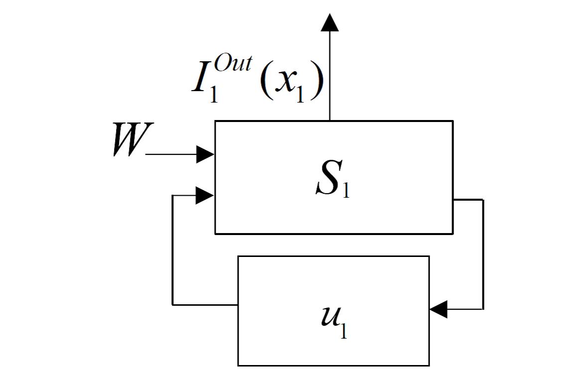
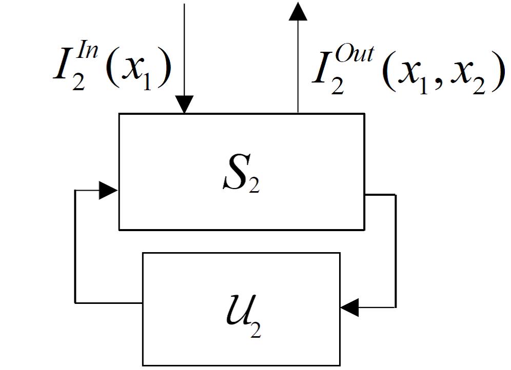
InterconnectionInterconnectionmissing-subexpressionmissing-subexpression\begin{array}[]{r@{\ }c@{\ }l}{\rm Interconnection}\end{array}
Refer to caption
(a)
Refer to caption
(b)
Refer to caption
(c)
Refer to caption
(d)
Figure 1: Distributed control systems with small random perturbations


whereS1:dx1(t)=m1(x1(t),u1(t))dt+ϵσ(x1(t))dW(t),Si:dxi(t)=mi(x1(t),x2(t),,xi(t),ui(t))dt,i=2,3,n,uj(t)=γjs(t,W(r),0rt),t[0,s],s0,j=1,2,n,IiIn(x1,x2,,xi1)andIiOut(x1,x2,,xi)are information for the expanding construction.missing-subexpressionmissing-subexpressionmissing-subexpressionwheremissing-subexpressionmissing-subexpressionmissing-subexpression:subscript𝑆1𝑑superscript𝑥1𝑡subscript𝑚1superscript𝑥1𝑡subscript𝑢1𝑡𝑑𝑡italic-ϵ𝜎superscript𝑥1𝑡𝑑𝑊𝑡missing-subexpressionmissing-subexpression:subscript𝑆𝑖formulae-sequence𝑑superscript𝑥𝑖𝑡subscript𝑚𝑖superscript𝑥1𝑡superscript𝑥2𝑡superscript𝑥𝑖𝑡subscript𝑢𝑖𝑡𝑑𝑡𝑖23𝑛missing-subexpressionmissing-subexpressionformulae-sequencesubscript𝑢𝑗𝑡superscriptsubscript𝛾𝑗𝑠𝑡𝑊𝑟0𝑟𝑡formulae-sequence𝑡0𝑠formulae-sequencefor-all𝑠0𝑗12𝑛missing-subexpressionmissing-subexpressionsuperscriptsubscript𝐼𝑖𝐼𝑛superscript𝑥1superscript𝑥2superscript𝑥𝑖1andsuperscriptsubscript𝐼𝑖𝑂𝑢𝑡superscript𝑥1superscript𝑥2superscript𝑥𝑖are information for the expanding construction.missing-subexpression\begin{array}[]{l@{\ }c@{\ }l}\\ \text{where}&\\ &S_{1}:\,\,dx^{1}(t)=m_{1}\bigl{(}x^{1}(t),u_{1}(t)\bigr{)}dt+\sqrt{\epsilon}\sigma\bigl{(}x^{1}(t)\bigr{)}dW(t),\\ &S_{i}:\,\,dx^{i}(t)=m_{i}\bigl{(}x^{1}(t),x^{2}(t),\ldots,x^{i}(t),u_{i}(t)\bigr{)}dt,~{}i=2,3,\ldots n,\\ &u_{j}(t)=\gamma_{j}^{s}\bigl{(}t,W(r),0\leq r\leq t\bigr{)},~{}t\in[0,\,s],~{}\forall s\geq 0,~{}j=1,2,\ldots n,\\ &I_{i}^{In}(x^{1},x^{2},\ldots,x^{i-1})~{}\text{and}~{}I_{i}^{Out}(x^{1},x^{2},\ldots,x^{i})~{}\text{are information for the expanding construction.}\end{array}

Remark 1

In general, the hypoellipticity is related to a strong accessibility property of controllable nonlinear systems that are driven by white noise (e.g., see SusJu72 concerning the controllability of nonlinear systems, which is closely related to StrVa72 and IchKu74 ). That is, the hypoellipticity assumption implies that the diffusion process x(t)superscript𝑥𝑡x^{\ell}(t) has a transition probability density p(t)((x1,,x),i=1dμi)p_{(t)}^{\ell}\bigl{(}(x^{1},\ldots,x^{\ell}),\otimes_{i=1}^{\ell}d\mu_{i}\bigr{)}, which is Csuperscript𝐶C^{\infty} on 2(d×)superscript2𝑑\mathbb{R}^{2(d\times\ell)}, with a strong Feller property.

Let Didsubscript𝐷𝑖superscript𝑑D_{i}\subset\mathbb{R}^{d}, for i=1,2,,n𝑖12𝑛i=1,2,\ldots,n, be bounded open domains with smooth boundaries (i.e., Disubscript𝐷𝑖\partial D_{i} is a manifold of class C2superscript𝐶2C^{2}). Moreover, let ΩsubscriptΩ\Omega_{\ell} be the open sets that are given by

Ω=D1×D2××D,{2,3,,n}.formulae-sequencesubscriptΩsubscript𝐷1subscript𝐷2subscript𝐷23𝑛\displaystyle\Omega_{\ell}=D_{1}\times D_{2}\times\cdots\times D_{\ell},\quad\ell\in\{2,3,\ldots,n\}.

Suppose that, for a fixed {2,3,,n}23𝑛\ell\in\{2,3,\ldots,n\}, the distributed control system, which is compatible with expanding construction, is formed by the first \ell subsystems (i.e., obtained by adding one after the other, until all \ellth subsystems are included). Furthermore, assume that the newly constructed distributed control system is composed with some admissible controls ui(t)𝒰isuperscriptsubscript𝑢𝑖𝑡subscript𝒰𝑖u_{i}^{\ast}(t)\in\mathcal{U}_{i}, t[0,)for-all𝑡0\forall t\in[0,\,\infty), for i=1,2,,1𝑖121i=1,2,\ldots,\ell-1. Let τϵ=τϵ(x1,x2,,x,u)superscriptsubscript𝜏italic-ϵsuperscriptsubscript𝜏italic-ϵsuperscript𝑥1superscript𝑥2superscript𝑥subscript𝑢\tau_{\ell}^{\epsilon}=\tau_{\ell}^{\epsilon}(x^{1},x^{2},\ldots,x^{\ell},u_{\ell}) be the exit-time for the diffusion process x(t)superscript𝑥𝑡x^{\ell}(t) (corresponding to the \ellth-subsystem), for a fixed ϵ>0italic-ϵ0\epsilon>0, with u𝒰subscript𝑢subscript𝒰u_{\ell}\in\mathcal{U}_{\ell}, from the given domain Dsubscript𝐷D_{\ell}, i.e.,

τϵ=inf{t>0|x(t)D},\displaystyle\tau_{\ell}^{\epsilon}=\inf\Bigl{\{}t>0\,\bigl{|}\,x^{\ell}(t)\notin D_{\ell}\Bigr{\}}, (8)

which depends on the behavior of the following (deterministic) distributed control system

dξ1(t)=m1(ξ1(t),u1(t))dtdξ2(t)=m2(ξ1(t),ξ2(t),u2(t))dtdξ1(t)=m1(ξ1(t),ξ2(t),,ξ1(t),u1(t))dtdξ(t)=m(ξ1(t),ξ2(t),,ξ(t),u(t))dt(ξ1(0),ξ2(0),,ξ(0))(x01,x02,,x0)Ω,t0}cases𝑑superscript𝜉1𝑡subscript𝑚1superscript𝜉1𝑡superscriptsubscript𝑢1𝑡𝑑𝑡𝑑superscript𝜉2𝑡subscript𝑚2superscript𝜉1𝑡superscript𝜉2𝑡superscriptsubscript𝑢2𝑡𝑑𝑡𝑑superscript𝜉1𝑡subscript𝑚1superscript𝜉1𝑡superscript𝜉2𝑡superscript𝜉1𝑡superscriptsubscript𝑢1𝑡𝑑𝑡𝑑superscript𝜉𝑡subscript𝑚superscript𝜉1𝑡superscript𝜉2𝑡superscript𝜉𝑡subscript𝑢𝑡𝑑𝑡formulae-sequencesuperscript𝜉10superscript𝜉20superscript𝜉0superscriptsubscript𝑥01superscriptsubscript𝑥02superscriptsubscript𝑥0subscriptΩ𝑡0\displaystyle\left.\begin{array}[]{l}d\xi^{1}(t)=m_{1}\bigl{(}\xi^{1}(t),u_{1}^{\ast}(t)\bigr{)}dt\\ d\xi^{2}(t)=m_{2}\bigl{(}\xi^{1}(t),\xi^{2}(t),u_{2}^{\ast}(t)\bigr{)}dt\\ \quad\quad\quad~{}\vdots\\ d\xi^{\ell-1}(t)=m_{\ell-1}\bigl{(}\xi^{1}(t),\xi^{2}(t),\ldots,\xi^{\ell-1}(t),u_{\ell-1}^{\ast}(t)\bigr{)}dt\\ d\xi^{\ell}(t)=m_{\ell}\bigl{(}\xi^{1}(t),\xi^{2}(t),\ldots,\xi^{\ell}(t),u_{\ell}(t)\bigr{)}dt\\ \bigl{(}\xi^{1}(0),\xi^{2}(0),\ldots,\xi^{\ell}(0)\bigr{)}\triangleq\bigl{(}x_{0}^{1},x_{0}^{2},\ldots,x_{0}^{\ell}\bigr{)}\in\Omega_{\ell},\,\,t\geq 0\end{array}\right\} (15)

In this paper, we specifically consider a risk-sensitive version of the mean escape time criterion with respect to the \ellth-subsystem, i.e.,

ϵlog𝔼x1,^ϵexp{1ϵθτϵ},italic-ϵsuperscriptsubscript𝔼subscript𝑥^1italic-ϵ1italic-ϵsubscript𝜃superscriptsubscript𝜏italic-ϵ\displaystyle-\epsilon\log\mathbb{E}_{x_{\widehat{1,\ell}}}^{\epsilon}\exp\biggl{\{}-\frac{1}{\epsilon}\theta_{\ell}\,\tau_{\ell}^{\epsilon}\biggr{\}}, (16)

where θsubscript𝜃\theta_{\ell}, for each {2,3,,n}23𝑛\ell\in\{2,3,\ldots,n\}, are positive design parameters and the expectation 𝔼x1,^ϵ{}superscriptsubscript𝔼subscript𝑥^1italic-ϵ\mathbb{E}_{x_{\widehat{1,\ell}}}^{\epsilon}\bigl{\{}\cdot\bigr{\}} is conditioned on the initial point (x01,x02,,x0)Ωsuperscriptsubscript𝑥01superscriptsubscript𝑥02superscriptsubscript𝑥0subscriptΩ\bigl{(}x_{0}^{1},x_{0}^{2},\ldots,x_{0}^{\ell}\bigr{)}\in\Omega_{\ell} as well as on the admissible controls (u1,u2,,u1,u)i=1𝒰isuperscriptsubscript𝑢1superscriptsubscript𝑢2superscriptsubscript𝑢1subscript𝑢superscriptsubscriptproduct𝑖1subscript𝒰𝑖\bigl{(}u_{1}^{\ast},u_{2}^{\ast},\ldots,u_{\ell-1}^{\ast},u_{\ell}\bigr{)}\in\prod\nolimits_{i=1}^{\ell}\mathcal{U}_{i}. Notice that τ1ϵsuperscriptsubscript𝜏1italic-ϵ\tau_{1}^{\epsilon} in the exit-time for the diffusion process x1(t)superscript𝑥1𝑡x^{1}(t) (which corresponds to the 111st-subsystem) from the domain D1subscript𝐷1D_{1} with respect to the admissible (optimal) control u1(t)𝒰1subscript𝑢1𝑡subscript𝒰1u_{1}(t)\in\mathcal{U}_{1}, t[0,)for-all𝑡0\forall t\in[0,\,\infty), with θ1>0subscript𝜃10\theta_{1}>0.222𝔼x1,^ϵ{}𝔼x1,x2,,x{}superscriptsubscript𝔼subscript𝑥^1italic-ϵsubscript𝔼superscript𝑥1superscript𝑥2superscript𝑥\mathbb{E}_{x_{\widehat{1,\ell}}}^{\epsilon}\bigl{\{}\cdot\bigr{\}}\triangleq\mathbb{E}_{x^{1},x^{2},\ldots,x^{\ell}}\bigl{\{}\cdot\bigr{\}}

Remark 2

Here we remark that the criterion in Equation (16) makes sense only if we have the following conditions

τ1ϵτ2ϵτϵ.superscriptsubscript𝜏1italic-ϵsuperscriptsubscript𝜏2italic-ϵsuperscriptsubscript𝜏italic-ϵ\displaystyle\tau_{1}^{\epsilon}\,\geq\,\tau_{2}^{\epsilon}\,\geq\,\cdots\,\geq\,\tau_{\ell}^{\epsilon}. (17)

Moreover, such conditions depend on the constituting subsystems, the admissible controls from the measurable sets i=1𝒰isuperscriptsubscriptproduct𝑖1subscript𝒰𝑖\prod_{i=1}^{\ell}\mathcal{U}_{i}, as well as on the given bounded open domains Disubscript𝐷𝑖D_{i}, for i=1,2,,𝑖12i=1,2,\ldots,\ell (see Section 3.2 for further discussion).

Then, the problem of risk-sensitive escape control (with respect to the \ellth-subsystem) will amount to obtaining a supremum value for V,θϵ=V,θϵ(x01,x02,,x0)superscriptsubscript𝑉subscript𝜃italic-ϵsuperscriptsubscript𝑉subscript𝜃italic-ϵsuperscriptsubscript𝑥01superscriptsubscript𝑥02superscriptsubscript𝑥0V_{\ell,\theta_{\ell}}^{\epsilon}=V_{\ell,\theta_{\ell}}^{\epsilon}\bigl{(}x_{0}^{1},x_{0}^{2},\ldots,x_{0}^{\ell}\bigr{)}, i.e.,

V,θϵsupu𝒰ϵlog𝔼x1,^ϵexp{1ϵθτϵ},superscriptsubscript𝑉subscript𝜃italic-ϵsubscriptsupremumsubscript𝑢subscript𝒰italic-ϵsuperscriptsubscript𝔼subscript𝑥^1italic-ϵ1italic-ϵsubscript𝜃superscriptsubscript𝜏italic-ϵ\displaystyle V_{\ell,\theta_{\ell}}^{\epsilon}\triangleq\sup_{u_{\ell}\in\mathcal{U}_{\ell}}-\epsilon\log\mathbb{E}_{x_{\widehat{1,\ell}}}^{\epsilon}\exp\biggl{\{}-\frac{1}{\epsilon}\theta_{\ell}\,\tau_{\ell}^{\epsilon}\biggr{\}}, (18)

with respect to some progressively measurable control u𝒰subscript𝑢subscript𝒰u_{\ell}\in\mathcal{U}_{\ell}, for each {2,3,,n}23𝑛\ell\in\{2,3,\ldots,n\}.

Notice that, for a fixed admissible control usubscript𝑢u_{\ell} from the measurable set  𝒰subscript𝒰\mathcal{U}_{\ell}, if we obtain a representation for Equation (16) as a minimal cost for an associated stochastic optimal control problem, then we will be able to obtain a representation for V,θϵsuperscriptsubscript𝑉subscript𝜃italic-ϵV_{\ell,\theta_{\ell}}^{\epsilon} as a value function for a stochastic differential game. This further allow us to link this progressively measurable control usubscript𝑢u_{\ell} in the original control problem with a strategy for the maximizing player of the associated stochastic differential game. Furthermore, such a connection between the risk-sensitive value function and a deterministic differential game can be made immediately, when the small random perturbation vanishes in the limit.

Before concluding this section, it is worth mentioning that some interesting studies on risk-sensitive control problem for dynamical systems with small random perturbations have been reported in literature (for example, see DupMc97 using PDE viscosity solution techniques; see BouDu01 using the probabilistic argumentation and the variational representation for degenerate diffusion processes; see also DaiMR96 , ElHam03 or FleMc95 for some connections between the risk-sensitive stochastic control and dynamic games).

An outline of the paper is as follows. In Section 2, we introduce a family of two-player differential games – where Player-111 will attempt to maximize the mean escape time criterion corresponding to each of the subsystems; while Player-222 will attempt to minimize it. In this section, we also provide some preliminary results that are useful for proving our main results. In Section 3, we present our main results – where we consider a risk-sensitive version of the mean escape time criterion with respect to each of the subsystems. Using the variational representation, we characterize the risk-sensitive escape control for the diffusion process as the lower and upper values of the associated stochastic differential game. Finally, we comment on the implication of our results, where one is also interested in evaluating the performance of the risk-sensitive escape control for the diffusion process, when there is some norm-bounded modeling error in the distributed control system.

2 Preliminary Results

2.1 A Differential Game Formalism

In this subsection, we consider a family of two-player differential games. For a fixed {2,3,,n}23𝑛\ell\in\{2,3,\ldots,n\}, at each time t[0,)𝑡0t\in[0,\,\infty), Player-111 picks a strategy u(t)subscript𝑢𝑡u_{\ell}(t) from the admissible control space 𝒰subscript𝒰\mathcal{U}_{\ell}, and Player-222 picks a control v(t)subscript𝑣𝑡v_{\ell}(t) from msuperscript𝑚\mathbb{R}^{m} in such a way that the functions tu(t)maps-to𝑡subscript𝑢𝑡t\mapsto u_{\ell}(t) and tv(t)maps-to𝑡subscript𝑣𝑡t\mapsto v_{\ell}(t) belong to the strategy sets

M={u:[0,)𝒰|uis progressively measurable}\displaystyle M_{\ell}=\biggl{\{}u_{\ell}\colon[0,\,\infty)\rightarrow\mathcal{U}_{\ell}\,\bigl{|}\,u_{\ell}\,\,\text{is progressively measurable}\biggr{\}} (19)

and

N={v:[0,)m|0T|v(t)|2dt<T<},\displaystyle N_{\ell}=\biggl{\{}v_{\ell}\colon[0,\,\infty)\rightarrow\mathbb{R}^{m}\,\biggl{|}\,\int_{0}^{T}\bigl{|}v_{\ell}(t)\bigr{|}^{2}dt<\infty\quad\forall T<\infty\biggr{\}}, (20)

respectively. Here, we also identify that Msubscript𝑀M_{\ell} and Nsubscript𝑁N_{\ell}, for any {2,3,,n}23𝑛\ell\in\{2,3,\ldots,n\}, as metric spaces under any metric which is equivalent to convergence in 2([0,T],ri)superscript20𝑇superscriptsubscript𝑟𝑖\mathscr{L}^{2}\bigl{(}[0,\,\ T],\mathbb{R}^{r_{i}}\bigr{)} and 2([0,T],m)superscript20𝑇superscript𝑚\mathscr{L}^{2}\bigl{(}[0,\,\ T],\mathbb{R}^{m}\bigr{)}.

Suppose that both players have played the game up to the (1)1(\ell-1)th-stage (see Footnote 4). Let ui(t)𝒰isuperscriptsubscript𝑢𝑖𝑡subscript𝒰𝑖u_{i}^{\ast}(t)\in\mathcal{U}_{i}, t[0,)for-all𝑡0\forall t\in[0,\,\infty), for i=1,2,,1𝑖121i=1,2,\ldots,\ell-1, be the admissible control strategies picked by the maximizing Player-111. Then, at the \ellth-stage, the dynamics of the game is given by the following differential equations

dx1(t)=m1(x1(t),u1(t))dt+σ(x1(t))v(t)dtdx2(t)=m2(x1(t),x2(t),u2(t))dtdx1(t)=m1(x1(t),x2(t),,x1(t),u1(t))dtdx(t)=m(x1(t),x2(t),,x(t),u(t))dt(x01,x02,,x0)Ω,t0}cases𝑑superscript𝑥1𝑡subscript𝑚1superscript𝑥1𝑡superscriptsubscript𝑢1𝑡𝑑𝑡𝜎superscript𝑥1𝑡subscript𝑣𝑡𝑑𝑡𝑑superscript𝑥2𝑡subscript𝑚2superscript𝑥1𝑡superscript𝑥2𝑡superscriptsubscript𝑢2𝑡𝑑𝑡𝑑superscript𝑥1𝑡subscript𝑚1superscript𝑥1𝑡superscript𝑥2𝑡superscript𝑥1𝑡superscriptsubscript𝑢1𝑡𝑑𝑡𝑑superscript𝑥𝑡subscript𝑚superscript𝑥1𝑡superscript𝑥2𝑡superscript𝑥𝑡subscript𝑢𝑡𝑑𝑡formulae-sequencesuperscriptsubscript𝑥01superscriptsubscript𝑥02superscriptsubscript𝑥0subscriptΩ𝑡0\displaystyle\left.\begin{array}[]{l}dx^{1}(t)=m_{1}\bigl{(}x^{1}(t),u_{1}^{\ast}(t)\bigr{)}dt+\sigma\bigl{(}x^{1}(t)\bigr{)}v_{\ell}(t)dt\\ dx^{2}(t)=m_{2}\bigl{(}x^{1}(t),x^{2}(t),u_{2}^{\ast}(t)\bigr{)}dt\\ \quad\quad\quad~{}\vdots\\ dx^{\ell-1}(t)=m_{\ell-1}\bigl{(}x^{1}(t),x^{2}(t),\ldots,x^{\ell-1}(t),u_{\ell-1}^{\ast}(t)\bigr{)}dt\\ dx^{\ell}(t)=m_{\ell}\bigl{(}x^{1}(t),x^{2}(t),\ldots,x^{\ell}(t),u_{\ell}(t)\bigr{)}dt\\ \quad\quad\quad\quad\quad\quad\quad\quad\quad\bigl{(}x_{0}^{1},x_{0}^{2},\ldots,x_{0}^{\ell}\bigr{)}\in\Omega_{\ell},\,\,t\geq 0\end{array}\right\} (27)

with an associated cost criterion

J(u,v)=120τ0|v(t)|2𝑑t+θτ0,subscript𝐽subscript𝑢subscript𝑣12superscriptsubscript0superscriptsubscript𝜏0superscriptsubscript𝑣𝑡2differential-d𝑡subscript𝜃superscriptsubscript𝜏0\displaystyle J_{\ell}\bigl{(}u_{\ell},v_{\ell}\bigr{)}=\frac{1}{2}\int_{0}^{\tau_{\ell}^{0}}\bigl{|}v_{\ell}(t)\bigr{|}^{2}dt+\theta_{\ell}\tau_{\ell}^{0}, (28)

where τ0inf{t>0|x(t)D}superscriptsubscript𝜏0infimumconditional-set𝑡0superscript𝑥𝑡subscript𝐷\tau_{\ell}^{0}\triangleq\inf\bigl{\{}t>0\,|\,x^{\ell}(t)\notin D_{\ell}\bigr{\}}. Note that the goal of Player-111 is to maximize Jsubscript𝐽J_{\ell} with respect to usubscript𝑢u_{\ell} and while that of Player-222 is to minimize it with respect to vsubscript𝑣v_{\ell}, for each {2,3,,n}23𝑛\ell\in\{2,3,\ldots,n\}. Here, we remark that Player-111 will attempt preventing the diffusion process x(t)superscript𝑥𝑡x^{\ell}(t) from leaving the given domain Dsubscript𝐷D_{\ell} (i.e., representing the exact control in risk-sensitive problem); while Player-222 will attempt forcing out the diffusion process from the domain (i.e., acting the role of the disturbance in the distributed control system).333We remark that the admissible control strategy usubscript𝑢u_{\ell} picked by Player-111 affects only the dynamics of the game, not directly the cost criterion.

Furthermore, a mapping α:NM:subscript𝛼subscript𝑁subscript𝑀\alpha_{\ell}\colon N_{\ell}\rightarrow M_{\ell} is said to be a strategy for the maximizing player if it is measurable and, for v,v^Nsubscript𝑣subscript^𝑣subscript𝑁v_{\ell},\,\hat{v}_{\ell}\in N_{\ell},

v(t)=v^(t),t[0,s]formulae-sequencesubscript𝑣𝑡subscript^𝑣𝑡for-all𝑡0𝑠\displaystyle v_{\ell}(t)=\hat{v}_{\ell}(t),\quad\forall t\in[0,\,s]

implies

α[v](t)=α[v^](t),t[0,s],formulae-sequencesubscript𝛼delimited-[]subscript𝑣𝑡subscript𝛼delimited-[]subscript^𝑣𝑡for-all𝑡0𝑠\displaystyle\alpha_{\ell}[v_{\ell}](t)=\alpha_{\ell}[\hat{v}_{\ell}](t),\quad\forall t\in[0,\,s],

almost everywhere, for every s[0,)𝑠0s\in[0,\,\infty).

Similarly, a mapping β:MN:subscript𝛽subscript𝑀subscript𝑁\beta_{\ell}\colon M_{\ell}\rightarrow N_{\ell} is a strategy for the minimizing player if it is measurable and, for u,u^Msubscript𝑢subscript^𝑢subscript𝑀u_{\ell},\,\hat{u}_{\ell}\in M_{\ell},

u(t)=u^(t),t[0,s]formulae-sequencesubscript𝑢𝑡subscript^𝑢𝑡for-all𝑡0𝑠\displaystyle u_{\ell}(t)=\hat{u}_{\ell}(t),\quad\forall t\in[0,\,s]

implies

β[u](t)=β[u^](t),t[0,s],formulae-sequencesubscript𝛽delimited-[]subscript𝑢𝑡subscript𝛽delimited-[]subscript^𝑢𝑡for-all𝑡0𝑠\displaystyle\beta_{\ell}[u_{\ell}](t)=\beta_{\ell}[\hat{u}_{\ell}](t),\quad\forall t\in[0,\,s],

almost everywhere, for every s[0,)𝑠0s\in[0,\,\infty).444Note that during each expanding construction (i.e., when a new subsystem is added to the existing distributed control system), we assume that both players play a differential game. For example, for =22\ell=2, the dynamics of the game is given by dx1(t)=m1(x1(t),u1(t))dt+σ(x1(t))v2(t)dtdx2(t)=m2(x1(t),x2(t),u2(t))dt(x01,x02)Ω2=D1×D2,t0,}cases𝑑superscript𝑥1𝑡subscript𝑚1superscript𝑥1𝑡superscriptsubscript𝑢1𝑡𝑑𝑡𝜎superscript𝑥1𝑡subscript𝑣2𝑡𝑑𝑡𝑑superscript𝑥2𝑡subscript𝑚2superscript𝑥1𝑡superscript𝑥2𝑡subscript𝑢2𝑡𝑑𝑡formulae-sequencesuperscriptsubscript𝑥01superscriptsubscript𝑥02subscriptΩ2subscript𝐷1subscript𝐷2𝑡0\displaystyle\left.\begin{array}[]{l}dx^{1}(t)=m_{1}\bigl{(}x^{1}(t),u_{1}^{\ast}(t)\bigr{)}dt+\sigma\bigl{(}x^{1}(t)\bigr{)}v_{2}(t)dt\\ dx^{2}(t)=m_{2}\bigl{(}x^{1}(t),x^{2}(t),u_{2}(t)\bigr{)}dt\\ \quad\quad\quad\quad\quad\bigl{(}x_{0}^{1},x_{0}^{2}\bigr{)}\in\Omega_{2}=D_{1}\times D_{2},\,\,t\geq 0,\end{array}\right\} with an associated cost criterion J2(u2,v2)=120τ20|v2(t)|2𝑑t+θ2τ20subscript𝐽2subscript𝑢2subscript𝑣212superscriptsubscript0superscriptsubscript𝜏20superscriptsubscript𝑣2𝑡2differential-d𝑡subscript𝜃2superscriptsubscript𝜏20\displaystyle J_{2}\bigl{(}u_{2},v_{2}\bigr{)}=\frac{1}{2}\int_{0}^{\tau_{2}^{0}}\bigl{|}v_{2}(t)\bigr{|}^{2}dt+\theta_{2}\tau_{2}^{0} and an exit-time τ20inf{t>0|x2(t)D2}superscriptsubscript𝜏20infimumconditional-set𝑡0superscript𝑥2𝑡subscript𝐷2\tau_{2}^{0}\triangleq\inf\bigl{\{}t>0\,|\,x^{2}(t)\notin D_{2}\bigr{\}} such that Player-111 optimally picks a strategy (in the sense of best-response correspondence) to the stagey of Player-222. Then, the game advances to the next stage, i.e., =33\ell=3, and continues until n𝑛n.

Let us denote the set of all maximizing strategies by ΓsubscriptΓ\Gamma_{\ell} and the set of all minimizing strategies by ΛsubscriptΛ\Lambda_{\ell}. Furthermore, let us define the lower and the upper values of the differential game at the \ellth-stage by

I(x01,x02,,x0)=infβΛsupuΓJ(u,v)superscriptsubscript𝐼superscriptsubscript𝑥01superscriptsubscript𝑥02superscriptsubscript𝑥0subscriptinfimumsubscript𝛽subscriptΛsubscriptsupremumsubscript𝑢subscriptΓsubscript𝐽subscript𝑢subscript𝑣\displaystyle I_{\ell}^{-}\bigl{(}x_{0}^{1},x_{0}^{2},\ldots,x_{0}^{\ell}\bigr{)}=\inf_{\beta_{\ell}\in\Lambda_{\ell}}\sup_{u_{\ell}\in\Gamma_{\ell}}J_{\ell}\bigl{(}u_{\ell},v_{\ell}\bigr{)} (29)

and

I+(x01,x02,,x0)=supuΓinfβΛJ(u,v),superscriptsubscript𝐼superscriptsubscript𝑥01superscriptsubscript𝑥02superscriptsubscript𝑥0subscriptsupremumsubscript𝑢subscriptΓsubscriptinfimumsubscript𝛽subscriptΛsubscript𝐽subscript𝑢subscript𝑣\displaystyle I_{\ell}^{+}\bigl{(}x_{0}^{1},x_{0}^{2},\ldots,x_{0}^{\ell}\bigr{)}=\sup_{u_{\ell}\in\Gamma_{\ell}}\inf_{\beta_{\ell}\in\Lambda_{\ell}}J_{\ell}\bigl{(}u_{\ell},v_{\ell}\bigr{)}, (30)

for each {2,3,,n}23𝑛{\ell}\in\{2,3,\ldots,n\}, respectively. Moreover, if

I(x01,x02,,x0)=I+(x01,x02,,x0),superscriptsubscript𝐼superscriptsubscript𝑥01superscriptsubscript𝑥02superscriptsubscript𝑥0superscriptsubscript𝐼superscriptsubscript𝑥01superscriptsubscript𝑥02superscriptsubscript𝑥0\displaystyle I_{\ell}^{-}\bigl{(}x_{0}^{1},x_{0}^{2},\ldots,x_{0}^{\ell}\bigr{)}=I_{\ell}^{+}\bigl{(}x_{0}^{1},x_{0}^{2},\ldots,x_{0}^{\ell}\bigr{)}, (31)

then the differential game has a value.

Remark 3

Note that the greatest payoff that Player-111 (i.e., the maximizing player) can force is called a lower value of the game and, similarly, the least value that Player-222 (i.e., the minimizing player) can force is termed an upper value of the game. In Section 3, we provide conditions under which these values coincide.

2.2 Additional Preliminary Results

In this subsection, we provide additional results that will be useful for proving our main results in Section 3.

Definition 1

We define 𝒱isubscript𝒱𝑖\mathscr{V}_{i} to be the set of all msuperscript𝑚\mathbb{R}^{m}-valued tsubscript𝑡\mathscr{F}_{t}-progressively measurable processes vi{vi(t),t[0,)}subscript𝑣𝑖subscript𝑣𝑖𝑡𝑡0v_{i}\triangleq\bigl{\{}v_{i}(t),\,t\in[0,\,\infty)\bigr{\}}, that satisfies

𝔼x1,^ϵ{0T|vi(t)|2𝑑t}<T<,formulae-sequencesuperscriptsubscript𝔼subscript𝑥^1italic-ϵsuperscriptsubscript0𝑇superscriptsubscript𝑣𝑖𝑡2differential-d𝑡for-all𝑇\displaystyle\mathbb{E}_{x_{\widehat{1,\ell}}}^{\epsilon}\biggl{\{}\int_{0}^{T}\bigl{|}v_{i}(t)\bigr{|}^{2}dt\biggr{\}}<\infty\quad\forall T<\infty,

for each i=1,2,,n𝑖12𝑛i=1,2,\ldots,n.

Lemma 1

[Variational representation formula (cf. (BouDu98, , Proposition 2.5 or Theorem 5.1))] For a fixed T<𝑇T<\infty, let f:𝒞([0,T],m):𝑓𝒞0𝑇superscript𝑚f\colon\mathscr{C}\bigl{(}[0,\,T],\mathbb{R}^{m}\bigr{)}\rightarrow\mathbb{R} be any Borel measurable bounded function. Then

log𝔼x1,^ϵexp{f(W)}=infv𝒱𝔼x1,^ϵ{120T|v(s)|2𝑑s+f(W+0v(s)𝑑s)},superscriptsubscript𝔼subscript𝑥^1italic-ϵ𝑓𝑊subscriptinfimumsubscript𝑣subscript𝒱superscriptsubscript𝔼subscript𝑥^1italic-ϵ12superscriptsubscript0𝑇superscriptsubscript𝑣𝑠2differential-d𝑠𝑓𝑊superscriptsubscript0subscript𝑣𝑠differential-d𝑠\displaystyle-\log\mathbb{E}_{x_{\widehat{1,\ell}}}^{\epsilon}\exp\biggl{\{}-f\bigl{(}W\bigr{)}\biggr{\}}=\inf_{v_{\ell}\in\mathscr{V}_{\ell}}\mathbb{E}_{x_{\widehat{1,\ell}}}^{\epsilon}\biggl{\{}\frac{1}{2}\int_{0}^{T}\bigl{|}v_{{\ell}}(s)\bigr{|}^{2}ds+f\biggl{(}W+\int_{0}^{\cdot}v_{{\ell}}(s)ds\biggr{)}\biggr{\}}, (32)

for any {2,3,,n}23𝑛{\ell}\in\{2,3,\ldots,n\}.

Lemma 2

For any v𝒱subscript𝑣subscript𝒱v_{\ell}\in\mathscr{V}_{\ell}, with {2,3,,n}23𝑛{\ell}\in\{2,3,\ldots,n\}, and T<𝑇T<\infty, let μvsuperscript𝜇subscript𝑣\mu^{v_{\ell}} be a measure induced on 𝒞([0,T],m)𝒞0𝑇superscript𝑚\mathscr{C}\bigl{(}[0,\,T],\mathbb{R}^{m}\bigr{)} by W+0v(t)𝑑t𝑊superscriptsubscript0subscript𝑣𝑡differential-d𝑡W+\int_{0}^{\cdot}v_{\ell}(t)dt under P𝑃P. Then, the relative entropy of μvsuperscript𝜇subscript𝑣\mu^{v_{\ell}} with respect to P𝑃P satisfies the following

(μvP)𝔼x1,^ϵ{0T|v(t)|2dt}.\displaystyle\mathcal{R}\bigl{(}\mu^{v_{\ell}}\bigl{\|}P\bigr{)}\leq\mathbb{E}_{x_{\widehat{1,\ell}}}^{\epsilon}\biggl{\{}\int_{0}^{T}\bigl{|}v_{\ell}(t)\bigr{|}^{2}dt\biggr{\}}. (33)

Let 𝒮𝒮\mathscr{S} a Polish space (i.e., a complete separable metric space), with a Borel σ𝜎\sigma-algebra, and let 𝒫(𝒮)𝒫𝒮\mathscr{P}(\mathscr{S}) be the set of measures defined on 𝒮𝒮\mathscr{S} that satisfies the usual hypotheses (e.g., see Kry80 ).

Lemma 3

[cf. (Bill68, , Theorem 2.1)] Consider a sequence of measures {μk,k}subscript𝜇𝑘𝑘\bigl{\{}\mu_{k},\,k\in\mathbb{N}\bigr{\}} in 𝒫(𝒮)𝒫𝒮\mathscr{P}(\mathscr{S}) satisfying

supk(μkP)<,\displaystyle\sup_{k\in\mathbb{N}}\mathcal{R}\bigl{(}\mu_{k}\bigl{\|}P\bigr{)}<\infty, (34)

where P𝒫(𝒮)𝑃𝒫𝒮P\in\mathscr{P}(\mathscr{S}). Let f:𝒮:𝑓𝒮f\colon\mathscr{S}\rightarrow\mathbb{R} be a Borel-measurable function. Then, the followings hold

  1. (i)

    if μksubscript𝜇𝑘\mu_{k} weakly converges to another measure μ𝜇\mu as k𝑘k\rightarrow\infty, then

    limk𝒮f𝑑μk=𝒮f𝑑μ,subscript𝑘subscript𝒮𝑓differential-dsubscript𝜇𝑘subscript𝒮𝑓differential-d𝜇\displaystyle\lim_{k\rightarrow\infty}\int_{\mathscr{S}}fd\mu_{k}=\int_{\mathscr{S}}fd\mu, (35)
  2. (ii)

    if {fk,k}subscript𝑓𝑘𝑘\bigl{\{}f_{k},\,k\in\mathbb{N}\bigr{\}} is a sequence of uniformly bounded functions that almost surely converges to f𝑓f, then

    limk𝒮fk𝑑μk=𝒮f𝑑μ.subscript𝑘subscript𝒮subscript𝑓𝑘differential-dsubscript𝜇𝑘subscript𝒮𝑓differential-d𝜇\displaystyle\lim_{k\rightarrow\infty}\int_{\mathscr{S}}f_{k}d\mu_{k}=\int_{\mathscr{S}}fd\mu. (36)

3 Main Results

3.1 Risk-Sensitive Escape Control Problem

In this subsection, we relate the lower and upper values of the associated differential game with the risk-sensitive escape control problem for the diffusion process. In particular, using the variational representation (e.g, see BouDu98 or DupMc97 ), we present our main results, i.e., Proposition 1 and Proposition 2.

For each fixed admissible control u𝒰subscript𝑢subscript𝒰u_{\ell}\in\mathcal{U}_{\ell}, the following proposition (which is a direct consequence of Lemma 1) characterizes the risk-sensitive escape control problem (cf. Equations (16) and (18)) with an associated stochastic differential game (cf. Equations (52) below).

Proposition 1

Suppose that, for a fixed {2,3,,n}23𝑛{\ell}\in\{2,3,\ldots,n\}, the admissible optimal controls ui(t)𝒰isuperscriptsubscript𝑢𝑖𝑡subscript𝒰𝑖u_{i}^{\ast}(t)\in\mathcal{U}_{i}, t[0,)for-all𝑡0\forall t\in[0,\,\infty), for i=1,2,,1𝑖121i=1,2,\ldots,\ell-1, are given. Consider any admissible control u𝒰subscript𝑢subscript𝒰u_{\ell}\in\mathcal{U}_{\ell}. Further, for every s[0,)𝑠0s\in[0,\,\infty), let γssuperscriptsubscript𝛾𝑠\gamma_{\ell}^{s} be a Borel measurable function such that u(t)=γs(t,W(r),0rt)subscript𝑢𝑡superscriptsubscript𝛾𝑠𝑡𝑊𝑟0𝑟𝑡u_{\ell}(t)=\gamma_{\ell}^{s}\bigl{(}t,W(r),0\leq r\leq t\bigr{)} for t[0,s]𝑡0𝑠t\in[0,\,s], w.p.1. Let the exit-time τϵsuperscriptsubscript𝜏italic-ϵ\tau_{\ell}^{\epsilon} be given by

τϵ=inf{t>0|x(t)D},\displaystyle\tau_{\ell}^{\epsilon}=\inf\bigl{\{}t>0\,\bigl{|}\,x^{\ell}(t)\notin D_{\ell}\bigr{\}},

which is associated with the following diffusion processes (x1,x2,,x)superscript𝑥1superscript𝑥2superscript𝑥\bigl{(}x^{1},x^{2},\ldots,x^{\ell}\bigr{)}, i.e.,

dx1(t)=m1(x1(t),u1(t))dt+ϵσ(x1(t))dW(t)dx2(t)=m2(x1(t),x2(t),u2(t))dtdx1(t)=m1(x1(t),x2(t),,x1(t),u1(t))dtdx(t)=m(x1(t),x2(t),,x(t),u(t))dt(x01,x02,,x0)Ω,t0}cases𝑑superscript𝑥1𝑡subscript𝑚1superscript𝑥1𝑡superscriptsubscript𝑢1𝑡𝑑𝑡italic-ϵ𝜎superscript𝑥1𝑡𝑑𝑊𝑡𝑑superscript𝑥2𝑡subscript𝑚2superscript𝑥1𝑡superscript𝑥2𝑡superscriptsubscript𝑢2𝑡𝑑𝑡𝑑superscript𝑥1𝑡subscript𝑚1superscript𝑥1𝑡superscript𝑥2𝑡superscript𝑥1𝑡superscriptsubscript𝑢1𝑡𝑑𝑡𝑑superscript𝑥𝑡subscript𝑚superscript𝑥1𝑡superscript𝑥2𝑡superscript𝑥𝑡subscript𝑢𝑡𝑑𝑡formulae-sequencesuperscriptsubscript𝑥01superscriptsubscript𝑥02superscriptsubscript𝑥0subscriptΩ𝑡0\displaystyle\left.\begin{array}[]{l}dx^{1}(t)=m_{1}\bigl{(}x^{1}(t),u_{1}^{\ast}(t)\bigr{)}dt+\sqrt{\epsilon}\sigma\bigl{(}x^{1}(t)\bigr{)}dW(t)\\ dx^{2}(t)=m_{2}\bigl{(}x^{1}(t),x^{2}(t),u_{2}^{\ast}(t)\bigr{)}dt\\ \quad\quad\quad~{}\vdots\\ dx^{\ell-1}(t)=m_{\ell-1}\bigl{(}x^{1}(t),x^{2}(t),\ldots,x^{\ell-1}(t),u_{\ell-1}^{\ast}(t)\bigr{)}dt\\ dx^{\ell}(t)=m_{\ell}\bigl{(}x^{1}(t),x^{2}(t),\ldots,x^{\ell}(t),u_{\ell}(t)\bigr{)}dt\\ \quad\quad\quad\quad\quad\quad\quad\quad\quad\bigl{(}x_{0}^{1},x_{0}^{2},\ldots,x_{0}^{\ell}\bigr{)}\in\Omega_{\ell},\,\,t\geq 0\end{array}\right\} (43)

Then, the following variational representation holds

ϵlog𝔼x1,^ϵexp{1ϵθτϵ}=infv𝒱𝔼x1,^ϵ{120τ~ϵ|v(s)|2𝑑s+θτ~ϵ},italic-ϵsuperscriptsubscript𝔼subscript𝑥^1italic-ϵ1italic-ϵsubscript𝜃superscriptsubscript𝜏italic-ϵsubscriptinfimumsubscript𝑣subscript𝒱superscriptsubscript𝔼subscript𝑥^1italic-ϵ12superscriptsubscript0superscriptsubscript~𝜏italic-ϵsuperscriptsubscript𝑣𝑠2differential-d𝑠subscript𝜃superscriptsubscript~𝜏italic-ϵ\displaystyle-\epsilon\log\mathbb{E}_{x_{\widehat{1,\ell}}}^{\epsilon}\exp\biggl{\{}-\frac{1}{\epsilon}\theta_{\ell}\,\tau_{\ell}^{\epsilon}\biggr{\}}=\inf_{v_{\ell}\in\mathscr{V}_{\ell}}\mathbb{E}_{x_{\widehat{1,\ell}}}^{\epsilon}\biggl{\{}\frac{1}{2}\int_{0}^{\tilde{\tau}_{\ell}^{\epsilon}}\bigl{|}v_{\ell}(s)\bigr{|}^{2}ds+\theta_{\ell}\tilde{\tau}_{\ell}^{\epsilon}\biggr{\}}, (44)

where the exit-time τ~ϵsuperscriptsubscript~𝜏italic-ϵ\tilde{\tau}_{\ell}^{\epsilon} is given by

τ~ϵ=inf{t>0|x~(t)D},\displaystyle\tilde{\tau}_{\ell}^{\epsilon}=\inf\Bigl{\{}t>0\,\bigl{|}\,\tilde{x}^{\ell}(t)\notin D_{\ell}\Bigr{\}}, (45)

which is associated with the following diffusion processes (x~1,x~2,,x~)superscript~𝑥1superscript~𝑥2superscript~𝑥\bigl{(}\tilde{x}^{1},\tilde{x}^{2},\ldots,\tilde{x}^{\ell}\bigr{)}, i.e.,

dx~1(t)=m1(x~1(t),u~1(t))dt+σ(x~1(t))v(t)dt+ϵσ(x~1(t))dW(t)dx~2(t)=m2(x~1(t),x~2(t),u~2(t))dtdx~1(t)=m1(x~1(t),x~2(t),,x~1(t),u~1(t))dtdx~(t)=m(x~1(t),x~2(t),,x~(t),u~(t))dt(x~1(0),x~2(0),,x~(0))(x01,x02,,x0)Ω,t0}cases𝑑superscript~𝑥1𝑡subscript𝑚1superscript~𝑥1𝑡superscriptsubscript~𝑢1𝑡𝑑𝑡𝜎superscript~𝑥1𝑡subscript𝑣𝑡𝑑𝑡italic-ϵ𝜎superscript~𝑥1𝑡𝑑𝑊𝑡𝑑superscript~𝑥2𝑡subscript𝑚2superscript~𝑥1𝑡superscript~𝑥2𝑡superscriptsubscript~𝑢2𝑡𝑑𝑡𝑑superscript~𝑥1𝑡subscript𝑚1superscript~𝑥1𝑡superscript~𝑥2𝑡superscript~𝑥1𝑡superscriptsubscript~𝑢1𝑡𝑑𝑡𝑑superscript~𝑥𝑡subscript𝑚superscript~𝑥1𝑡superscript~𝑥2𝑡superscript~𝑥𝑡subscript~𝑢𝑡𝑑𝑡formulae-sequencesuperscript~𝑥10superscript~𝑥20superscript~𝑥0superscriptsubscript𝑥01superscriptsubscript𝑥02superscriptsubscript𝑥0subscriptΩ𝑡0\displaystyle\left.\begin{array}[]{l}d\tilde{x}^{1}(t)=m_{1}\bigl{(}\tilde{x}^{1}(t),\tilde{u}_{1}^{\ast}(t)\bigr{)}dt+\sigma\bigl{(}\tilde{x}^{1}(t))v_{\ell}(t)dt+\sqrt{\epsilon}\sigma\bigl{(}\tilde{x}^{1}(t))dW(t)\\ d\tilde{x}^{2}(t)=m_{2}\bigl{(}\tilde{x}^{1}(t),\tilde{x}^{2}(t),\tilde{u}_{2}^{\ast}(t)\bigr{)}dt\\ \quad\quad\quad~{}\vdots\\ d\tilde{x}^{\ell-1}(t)=m_{\ell-1}\bigl{(}\tilde{x}^{1}(t),\tilde{x}^{2}(t),\ldots,\tilde{x}^{\ell-1}(t),\tilde{u}_{\ell-1}^{\ast}(t)\bigr{)}dt\\ d\tilde{x}^{\ell}(t)=m_{\ell}\bigl{(}\tilde{x}^{1}(t),\tilde{x}^{2}(t),\ldots,\tilde{x}^{\ell}(t),\tilde{u}_{\ell}(t)\bigr{)}dt\\ \bigl{(}\tilde{x}^{1}(0),\tilde{x}^{2}(0),\ldots,\tilde{x}^{\ell}(0)\bigr{)}\triangleq\bigl{(}x_{0}^{1},x_{0}^{2},\ldots,x_{0}^{\ell}\bigr{)}\in\Omega_{\ell},\,\,t\geq 0\end{array}\right\} (52)

Moreover, the admissible control u~subscript~𝑢\tilde{u}_{\ell} satisfies

u~(t)=γs(t,W(r)+1ϵ0rv(z)𝑑z,0rt),t[0,s],w.p.1,formulae-sequencesubscript~𝑢𝑡superscriptsubscript𝛾𝑠𝑡𝑊𝑟1italic-ϵsuperscriptsubscript0𝑟subscript𝑣𝑧differential-d𝑧0𝑟𝑡for-all𝑡0𝑠w.p.1\displaystyle\tilde{u}_{\ell}(t)=\gamma_{\ell}^{s}\biggl{(}t,W(r)+\frac{1}{\sqrt{\epsilon}}\int_{0}^{r}v_{\ell}(z)dz,0\leq r\leq t\biggr{)},\quad\forall t\in[0,\,s],\quad\text{w.p.1}, (53)

for any s[0,)𝑠0s\in[0,\,\infty).

The following proposition provides conditions under which the lower and upper values of the associated differential game (i.e., quantities in Equations (29) and (30)) will coincide.

Proposition 2

For a fixed {2,3,,n}23𝑛{\ell}\in\{2,3,\ldots,n\}, let I(x01,x02,,x0)superscriptsubscript𝐼superscriptsubscript𝑥01superscriptsubscript𝑥02superscriptsubscript𝑥0I_{\ell}^{-}\bigl{(}x_{0}^{1},x_{0}^{2},\ldots,x_{0}^{\ell}\bigr{)} and I+(x01,x02,,x0)superscriptsubscript𝐼superscriptsubscript𝑥01superscriptsubscript𝑥02superscriptsubscript𝑥0I_{\ell}^{+}\bigl{(}x_{0}^{1},x_{0}^{2},\ldots,x_{0}^{\ell}\bigr{)} be the lower and upper values of the associated differential game given in Equations (29) and (30). Suppose that ui(t)𝒰isuperscriptsubscript𝑢𝑖𝑡subscript𝒰𝑖u_{i}^{\ast}(t)\in\mathcal{U}_{i}, t[0,)for-all𝑡0\forall t\in[0,\,\infty), for i=1,2,,1𝑖121i=1,2,\ldots,\ell-1, are admissible optimal controls. For any u𝒰subscript𝑢subscript𝒰u_{\ell}\in\mathcal{U}_{\ell}, let (x1,x2,,x)superscript𝑥1superscript𝑥2superscript𝑥\bigl{(}x^{1},x^{2},\ldots,x^{\ell}\bigr{)} be the unique solution to Equation (43). Then,

  1. (i)

    the lower value of the game satisfies

    lim supϵ0supu𝒰ϵlog𝔼x1,^ϵexp{1ϵθτϵ}I(x01,x02,,x0),subscriptlimit-supremumitalic-ϵ0subscriptsupremumsubscript𝑢subscript𝒰italic-ϵsuperscriptsubscript𝔼subscript𝑥^1italic-ϵ1italic-ϵsubscript𝜃superscriptsubscript𝜏italic-ϵsuperscriptsubscript𝐼superscriptsubscript𝑥01superscriptsubscript𝑥02superscriptsubscript𝑥0\displaystyle\limsup_{\epsilon\rightarrow 0}\sup_{u_{\ell}\in\mathcal{U}_{\ell}}-\epsilon\log\mathbb{E}_{x_{\widehat{1,\ell}}}^{\epsilon}\exp\biggl{\{}-\frac{1}{\epsilon}\theta_{\ell}\,\tau_{\ell}^{\epsilon}\biggr{\}}\leq I_{\ell}^{-}\bigl{(}x_{0}^{1},x_{0}^{2},\ldots,x_{0}^{\ell}\bigr{)}, (54)
  2. (ii)

    for a given κ>0𝜅0\kappa>0, there exists a measurable function g:𝒞([0,T],m)M:subscript𝑔𝒞0𝑇superscript𝑚subscript𝑀g_{\ell}\colon\mathscr{C}\bigl{(}[0,\,T],\mathbb{R}^{m}\bigr{)}\rightarrow M_{\ell} such that the upper value of the game satisfies

    lim infϵ0supu𝒰ϵlog𝔼x1,^ϵexp{1ϵθτϵ}I+(x01,x02,,x0)κ,subscriptlimit-infimumitalic-ϵ0subscriptsupremumsubscript𝑢subscript𝒰italic-ϵsuperscriptsubscript𝔼subscript𝑥^1italic-ϵ1italic-ϵsubscript𝜃superscriptsubscript𝜏italic-ϵsuperscriptsubscript𝐼superscriptsubscript𝑥01superscriptsubscript𝑥02superscriptsubscript𝑥0𝜅\displaystyle\liminf_{\epsilon\rightarrow 0}\sup_{u_{\ell}\in\mathcal{U}_{\ell}}-\epsilon\log\mathbb{E}_{x_{\widehat{1,\ell}}}^{\epsilon}\exp\biggl{\{}-\frac{1}{\epsilon}\theta_{\ell}\,\tau_{\ell}^{\epsilon}\biggr{\}}\geq I_{\ell}^{+}\bigl{(}x_{0}^{1},x_{0}^{2},\ldots,x_{0}^{\ell}\bigr{)}-\kappa, (55)

    with u=g[ϵW]subscript𝑢subscript𝑔delimited-[]italic-ϵ𝑊u_{\ell}=g_{\ell}[\sqrt{\epsilon}W] (i.e., when the maximizing player picks such a strategy),

  3. (iii)

    if the lower and upper values of the game coincides, i.e.,

    I(x01,x02,,x0)=I+(x01,x02,,x0),superscriptsubscript𝐼superscriptsubscript𝑥01superscriptsubscript𝑥02superscriptsubscript𝑥0superscriptsubscript𝐼superscriptsubscript𝑥01superscriptsubscript𝑥02superscriptsubscript𝑥0\displaystyle I_{\ell}^{-}\bigl{(}x_{0}^{1},x_{0}^{2},\ldots,x_{0}^{\ell}\bigr{)}=I_{\ell}^{+}\bigl{(}x_{0}^{1},x_{0}^{2},\ldots,x_{0}^{\ell}\bigr{)}, (56)

    then the game has a value.

3.2 Remarks on the Robust Analysis Problem

In this subsection, we briefly remark on the implication of our main results – where one is also interested in evaluating the robust performance of the risk-sensitive escape control, when there is some norm-bounded modeling error in the distributed control system (see DupJaPe00 for related discussion, but in different context).

In what follows, we assume that that the statements in Propositions 1 and 2 are true. Suppose that, for a fixed {2,3,,n}23𝑛{\ell}\in\{2,3,\ldots,n\}, ui(t)𝒰isuperscriptsubscript𝑢𝑖𝑡subscript𝒰𝑖u_{i}^{\ast}(t)\in\mathcal{U}_{i}, t[0,)for-all𝑡0\forall t\in[0,\,\infty), for i=1,2,,𝑖12i=1,2,\ldots,\ell, are the admissible optimal control strategies picked by Player-111. Further, we consider the following distributed control system (which contains \ell subsystems)

dx^1(t)=m1(x^1(t),u1(t))dt+σ(x^1(t))v^(t)dtdx^2(t)=m2(x^1(t),u2(t),u^2(t))dtdx^(t)=m(x^1(t),x^2(t),,x^(t),u(t))dt(x^1(0),x^2(0),,x^(0))(x01,x02,,x0)Ω,t0}cases𝑑superscript^𝑥1𝑡subscript𝑚1superscript^𝑥1𝑡superscriptsubscript𝑢1𝑡𝑑𝑡𝜎superscript^𝑥1𝑡subscript^𝑣𝑡𝑑𝑡𝑑superscript^𝑥2𝑡subscript𝑚2superscript^𝑥1𝑡superscriptsubscript𝑢2𝑡subscript^𝑢2𝑡𝑑𝑡𝑑superscript^𝑥𝑡subscript𝑚superscript^𝑥1𝑡superscript^𝑥2𝑡superscript^𝑥𝑡superscriptsubscript𝑢𝑡𝑑𝑡formulae-sequencesuperscript^𝑥10superscript^𝑥20superscript^𝑥0superscriptsubscript𝑥01superscriptsubscript𝑥02superscriptsubscript𝑥0subscriptΩ𝑡0\displaystyle\left.\begin{array}[]{l}d\hat{x}^{1}(t)=m_{1}\bigl{(}\hat{x}^{1}(t),{u}_{1}^{\ast}(t)\bigr{)}dt+\sigma\bigl{(}\hat{x}^{1}(t))\hat{v}_{\ell}(t)dt\\ d\hat{x}^{2}(t)=m_{2}\bigl{(}\hat{x}^{1}(t),{u}_{2}^{\ast}(t),\hat{u}_{2}(t)\bigr{)}dt\\ \quad\quad\quad~{}\vdots\\ d\hat{x}^{\ell}(t)=m_{\ell}\bigl{(}\hat{x}^{1}(t),\hat{x}^{2}(t),\ldots,\hat{x}^{\ell}(t),{u}_{\ell}^{\ast}(t)\bigr{)}dt\\ \quad\bigl{(}\hat{x}^{1}(0),\hat{x}^{2}(0),\ldots,\hat{x}^{\ell}(0)\bigr{)}\triangleq\bigl{(}x_{0}^{1},x_{0}^{2},\ldots,x_{0}^{\ell}\bigr{)}\in\Omega_{\ell},\,\,t\geq 0\end{array}\right\} (62)

where v^(t)Nsubscript^𝑣𝑡subscript𝑁\hat{v}_{\ell}(t)\in N_{\ell}.

Define the value function V,θ0=V,θ0(x01,x02,,x0)superscriptsubscript𝑉subscript𝜃0superscriptsubscript𝑉subscript𝜃0superscriptsubscript𝑥01superscriptsubscript𝑥02superscriptsubscript𝑥0V_{\ell,\theta_{\ell}}^{0}=V_{\ell,\theta_{\ell}}^{0}\bigl{(}x_{0}^{1},x_{0}^{2},\ldots,x_{0}^{\ell}\bigr{)} as

V,θ0infv^N{120τ0|v^(t)|2𝑑t+θτ0},superscriptsubscript𝑉subscript𝜃0subscriptinfimumsubscript^𝑣subscript𝑁12superscriptsubscript0superscriptsubscript𝜏0superscriptsubscript^𝑣𝑡2differential-d𝑡subscript𝜃superscriptsubscript𝜏0\displaystyle V_{\ell,\theta_{\ell}}^{0}\triangleq\inf_{\hat{v}_{\ell}\in N_{\ell}}\biggl{\{}\frac{1}{2}\int_{0}^{\tau_{\ell}^{0}}\bigl{|}\hat{v}_{\ell}(t)\bigr{|}^{2}dt+\theta_{\ell}\tau_{\ell}^{0}\biggr{\}}, (63)

where τ0=inf{t>0|x(t)D}superscriptsubscript𝜏0infimumconditional-set𝑡0superscript𝑥𝑡subscript𝐷\tau_{\ell}^{0}=\inf\bigl{\{}t>0\,|\,x^{\ell}(t)\notin D_{\ell}\bigr{\}}, with θ>0subscript𝜃0\theta_{\ell}>0. Then, for any v^Nsubscript^𝑣subscript𝑁\hat{v}_{\ell}\in N_{\ell}, with v^<subscriptdelimited-∥∥subscript^𝑣\bigl{\|}\hat{v}_{\ell}\bigr{\|}_{\infty}<\infty, we have the following inequalities

V,θ0superscriptsubscript𝑉subscript𝜃0\displaystyle V_{\ell,\theta_{\ell}}^{0} 120τ0|v^(t)|2𝑑t+θτ0,absent12superscriptsubscript0superscriptsubscript𝜏0superscriptsubscript^𝑣𝑡2differential-d𝑡subscript𝜃superscriptsubscript𝜏0\displaystyle\leq\frac{1}{2}\int_{0}^{\tau_{\ell}^{0}}\bigl{|}\hat{v}_{\ell}(t)\bigr{|}^{2}dt+\theta_{\ell}\tau_{\ell}^{0},
τ02v^2+θτ0absentsuperscriptsubscript𝜏02superscriptsubscriptdelimited-∥∥subscript^𝑣2subscript𝜃superscriptsubscript𝜏0\displaystyle\leq\frac{\tau_{\ell}^{0}}{2}\bigl{\|}\hat{v}_{\ell}\bigr{\|}_{\infty}^{2}+\theta_{\ell}\tau_{\ell}^{0} (64)

and

τ0V,θ012v^2+θ.superscriptsubscript𝜏0superscriptsubscript𝑉subscript𝜃012superscriptsubscriptdelimited-∥∥subscript^𝑣2subscript𝜃\displaystyle\tau_{\ell}^{0}\geq\frac{V_{\ell,\theta_{\ell}}^{0}}{\frac{1}{2}\bigl{\|}\hat{v}_{\ell}\bigr{\|}_{\infty}^{2}+\theta_{\ell}}. (65)

Suppose that v^(t)Δm(t)subscript^𝑣𝑡Δsubscript𝑚𝑡\hat{v}_{\ell}(t)\triangleq\Delta m_{\ell}(t), where Δm(t)Δsubscript𝑚𝑡\Delta m_{\ell}(t) is interpreted as a modeling error in Equation (56). Further, assume that the value τ0superscriptsubscript𝜏0\tau_{\ell}^{0} is used as a qualitative measure on the performance of the distributed control system. For a given specification Lsubscript𝐿L_{\ell}, with τ0Lsuperscriptsubscript𝜏0subscript𝐿\tau_{\ell}^{0}\geq L_{\ell}, if there exists a design parameter θ>0superscriptsubscript𝜃0\theta_{\ell}^{\ast}>0 such that

V,θ0θ>L.superscriptsubscript𝑉superscriptsubscript𝜃0superscriptsubscript𝜃subscript𝐿\displaystyle\frac{V_{\ell,\theta_{\ell}^{\ast}}^{0}}{\theta_{\ell}^{\ast}}>L_{\ell}. (66)

Then, we obtain an upper bound on the norm of the modeling error, which guarantees the desired performance against all modeling errors satisfying such a norm bound. That is, if

Δm22[V,θ0Lθ],superscriptsubscriptdelimited-∥∥Δsubscript𝑚22delimited-[]superscriptsubscript𝑉superscriptsubscript𝜃0subscript𝐿superscriptsubscript𝜃\displaystyle\bigl{\|}\Delta m_{\ell}\bigr{\|}_{\infty}^{2}\leq 2\left[\frac{V_{\ell,\theta_{\ell}^{\ast}}^{0}}{L_{\ell}}-\theta_{\ell}^{\ast}\right], (67)

then we have

τ0V,θ012Δm2+θL.superscriptsubscript𝜏0superscriptsubscript𝑉superscriptsubscript𝜃012superscriptsubscriptdelimited-∥∥Δsubscript𝑚2superscriptsubscript𝜃subscript𝐿\displaystyle\tau_{\ell}^{0}\geq\frac{V_{\ell,\theta_{\ell}^{\ast}}^{0}}{\frac{1}{2}\bigl{\|}\Delta m_{\ell}\bigr{\|}_{\infty}^{2}+\theta_{\ell}^{\ast}}\geq L_{\ell}. (68)

Moreover, the above equation (together with Equation (17)) further implies the following

Vi,θi012Δmi2+θiVi+1,θi+1012Δmi+12+θi+1,superscriptsubscript𝑉𝑖superscriptsubscript𝜃𝑖012superscriptsubscriptdelimited-∥∥Δsubscript𝑚𝑖2superscriptsubscript𝜃𝑖superscriptsubscript𝑉𝑖1superscriptsubscript𝜃𝑖1012superscriptsubscriptdelimited-∥∥Δsubscript𝑚𝑖12superscriptsubscript𝜃𝑖1\displaystyle\frac{V_{i,\theta_{i}^{\ast}}^{0}}{\frac{1}{2}\bigl{\|}\Delta m_{i}\bigr{\|}_{\infty}^{2}+\theta_{i}^{\ast}}\geq\frac{V_{i+1,\theta_{i+1}^{\ast}}^{0}}{\frac{1}{2}\bigl{\|}\Delta m_{i+1}\bigr{\|}_{\infty}^{2}+\theta_{i+1}^{\ast}}, (69)

for i=1,2,,1𝑖121i=1,2,\ldots,\ell-1, with {2,3,,n}23𝑛\ell\in\{2,3,\ldots,n\}.

Remark 4

Note that, for each i=1,2,,n𝑖12𝑛i=1,2,\ldots,n, the norm on the modeling error is inversely proportional to the design specification Lisubscript𝐿𝑖L_{i}, and, therefore, the robustness of the distributed control system increases as the bound on the performance measure decreases.

References

  • (1) Befekadu GK, Antsaklis PJ (2014) On the minimum exit rate for a diffusion process pertaining to a chain of distributed control systems with random perturbations. arXiv:1408.6260 [math.CT]
  • (2) Billingsley P (1968) Convergence of probability measures. Wiley, New York
  • (3) Boué M, Dupuis P (1998) A variational representation for certain functionals of Brownian motion. Ann Probab 26:1641–1659
  • (4) Boué M, Dupuis P (2001) Risk-sensitive and robust escape control for degenerate diffusion processes. Math Contr Sign Sys 14:62–85
  • (5) Dai Pra P, Meneghini L, Runggaldier WJ (1996) Some connections between stochastic control and dynamic games. Math Contr Sig Sys 9:303–326
  • (6) Dupuis P, James MR, Petersen I (2000) Robust properties of risk-sensitive control. Math Contr Sig Sys 13:318–332
  • (7) Dupuis P, Kushner HJ (1989) Minimizing escape probabilities: a large deviations approach. SIAM J Control Optim 27:432–445
  • (8) Dupuis P, McEneaney WM (1997) Risk-sensitive and robust escape criteria. SIAM J Control Optim 35:2021–2049
  • (9) El-Karouia N, Hamadène S (2003) BSDEs and risk-sensitive control, zero-sum and nonzero-sum game problems of stochastic functional differential equations. Stochastic Processes Appl 107:145–169
  • (10) Elliott DL (1973) Diffusions on manifolds arising from controllable systems. in: Geometric methods in system theory, Mayne DQ, Brockett RW, eds. Reidel Publ. Co., Dordrecht, Holland, 285–294
  • (11) Fleming WH, McEneaney WM (1995) Risk sensitive control on an infinite time horizon. SIAM J Control Optim 33:1881–1915
  • (12) Hörmander L (1967) Hypoelliptic second order differential operators. Acta Math 119:147–171
  • (13) Ichihara K, Kunita H (1974) A classification of the second order degenerate elliptic operators and its probabilistic characterization. Z Wahrscheinlichkeitstheor Verw Geb 30:253–254
  • (14) Karatzas I, Shreve SE (1988) Brownian motion and stochastic calculus. Springer-Verlag, New York
  • (15) Krylov NV (1980) Controlled diffusion processes. Springer-Verlag, New York
  • (16) Stroock D, Varadhan SRS (1972) On degenerate elliptic-parabolic operators of second order and their associated diffusions. Comm Pure Appl Math 25:651–713
  • (17) Sussmann HJ, Jurdjevic V (1972) Controllability of nonlinear systems. J Diff Equ 12:95–116