The Lyman- forest as a cosmic thermometer
Abstract
We present a comprehensive analysis of high resolution hydrodynamic simulations in terms of Lyman- and Lyman- one dimensional flux power spectra ( and ). In particular, we focus on the behaviour that the flux auto-power spectra and cross-power spectra () display when the intergalactic medium (IGM) thermal history is changed in a range of values that bracket a reference model, while cosmological parameters are kept fixed to best fit the cosmic microwave background data. We present empirical fits that describe at the sub-percent level the dependence of the power spectra on the thermal parameters. At the largest scales, the power spectra show a constant bias between each other that is set by the parameters describing the IGM thermal state. The cross-power spectrum has an oscillatory pattern and crosses zero at a scale which depends on , the IGM temperature at the mean density, for reasonable values of the power-law index of the IGM temperature-density relation (). By performing a Fisher matrix analysis, we find that the power spectrum is more sensitive to the thermal history than alone, due to the fact that it probes denser regions than Lyman-Ẇhen we combine the power and cross spectra the constraints on can be improved by a factor , while the constraints on improve by a factor of . We address the role of signal-to-noise and resolution by mocking realistic observations and we conclude that the framework presented in this work can significantly improve the knowledge of the IGM thermal state, which will in turn guarantee better constraints on IGM-derived cosmological parameters.
1 Introduction
The last decade has witnessed an enormous progress in the cosmological investigation of the intergalactic medium (IGM) as probed by the Lyman- forest (see [1, 2] for reviews). In particular, the Lyman- forest is now a viable cosmological observable that can help in putting constraints on cosmological parameters and/or deviations from a standard scenario based on cold dark matter and a cosmological constant. Several statistics of the transmitted flux can be considered. For example, the one-dimensional (1D) Lyman- flux power spectrum [3, 4, 5, 6, 7, 8, 9], as derived from both high and low-resolution data, is the quantity that has been widely used in order to place constraints on the amplitude and slope of the linear matter power spectrum in a unique range of redshifts and scales [5, 10, 7]. This has in turn allowed to put tight limits on fundamental quantities like inflationary parameters, cold dark matter coldness and neutrino masses [11, 12], especially when these data are combined with large scale information like the cosmic microwave background and galaxy clustering. Basically, any physical effect, like for example modified gravity, happening at scales of comoving Mpc will impact dramatically on the Lyman- forest properties as probed by the 1D flux power. More recently, the very large number of quasar spectra of the SDSS-III/BOSS (Sloan Digital Sky Survey-III/Baryon Oscillation Spectroscopic Survey) collaboration using a state-of-the-art analysis, has allowed to discover Baryonic Acoustic Oscillations (BAOs) in the transmitted Lyman- flux at [13, 14]: this spectacular confirmation of the cosmological nature of the Lyman- forest was mainly made possible by exploiting the flux correlations in three dimensions out to large scales.
What is usually not fully appreciated is that final cosmologically relevant numbers are obtained by running a relatively sophisticated pipeline that marginalizes over the many nuisance and/or astrophysical parameters affecting the investigated IGM observable. The parameters describing the physics of the IGM are in principal many, since the physics is rich and affected by astrophysical properties of the surrounding galaxies (e.g. galactic feedback in the form of galactic winds or Active Galactic Nuclei or Blazar heating [15, 16, 17]), or by the presence of strong systems that are usually associated with dense environments which are difficult to model [18, 15], or reionization and complex radiative transfer effects impacting on the low density IGM [19].
However, there are more obvious parameters that are also constrained independently by different techniques: those governing the so-called “equation-of-state” of the IGM. This relation is often assumed to be adiabatic in form, connecting the temperature () to the baryon density :
| (1.1) |
where is critical density of the Universe at a given redshift and is the baryon density contrast. The parameters are and , governing the mean temperature of the IGM and the slope of the relation, respectively [20, 21]. Note that these parameters have been constrained in a series of works by using: line-fitting procedures [22, 23, 24, 25], wavelet analysis [26, 27, 28, 29], flux probability distribution function [30, 31], flux power spectrum [3, 32], and curvature of the transmitted flux [33, 34]. All these different methods provide constraints (at different redshifts and probing slightly different density regimes) with still relatively large error bars.
While degeneracies are intrinsically present in the Lyman- forest analysis, one can hope that with better constraints on the parameters of the IGM, the strength of the degeneracy can be lifted. To break up this degeneracy several studies have suggested to use either higher order statistics of the Lyman- forest (such as bispectrum, flux pdf, wavelet) (see e.g. [35]) or higher order neutral hydrogen transitions (such as Lyman- or Lyman- transitions), or to exploit the (possibly different) redshift dependence of cosmological and astrophysical effects by using a wider redshift range (e.g. like in BOSS as analyzed by [10]).
Using only Lyman- forest to determine the IGM parameters is difficult since the Lyman- cross section is large enough to produce saturated absorption fast. The Lyman- forest presents an opportunity to measure the same large-scale structure of Lyman- but with a different sensitivity to the optical depth of the photons travelling through the IGM. In other terms, Lyman- forest is an additional measurement of the IGM and large scale structure but with different bias parameters. However, since the bias relationship between the observed flux and the optical depth is highly nonlinear, the relationship between the and is not trivial.
So far the gain of using the Lyman- forest has been estimated using dark matter N-body simulations [36]. On the data side, a recent investigation of Lyman- flux power spectrum, and the cross spectrum using BOSS data has been presented in [37]. Even though these findings provide convincing indications that using the Lyman- forest statistics should alleviate the tensions between IGM parameters and cosmology, a more complete and precise assessment using hydrodynamical simulation is deemed necessary. In this respect, the present work is an improvement of the already existing analysis with the important new ingredient of probing also the cross-spectrum between Lyman- and Lyman-.
The paper is structured as follows: in Section 2 we describe the hydrodynamic simulations used; in Section 3 we discuss how we model the Lyman- absorption; Section 4 contains our results in terms of auto and cross spectra together with a quantitative analysis of their dependence on the thermal state; Section 5 presents the Fisher Matrix analysis of the power spectra; Section 6 summarizes our findings.
2 Hydrodynamic Simulations and Spectra Analysis
The grid of simulations used in the present analysis is performed by using the Tree-Particle Mesh (PM) Smoothed Particle Hydrodynamics (SPH) code GADGET-III [38]. Star formation is followed by using a simplified procedure (commonly denoted QUICKLY), employed for the first time in [7], which turns gas particles with overdensity larger than 1000 and temperature below K into stars. This procedure has been shown to provide sub-percent level accuracy in terms of Lyman- statistics when compared to the more refined effective model for the inter-stellar medium [7]. The cooling routines have been slightly modified in order to achieve a given thermal history at the desired redshift as done recently in [39], where the grid of thermal histories explored in the present work is also presented. Thereby, we do not make an a-posteriori scaling of the temperature density relation but our thermal histories have been obtained consistently within the SPH simulations. Our reference thermal history is tailored to match the recent curvature-based measurements of presented in [33].
The simulated cosmological periodic volume has a linear size of , gas particles and dark matter particles (the mass per gas particle is ). The cosmological parameters, kept fixed, have the following values: , , , , km/s/Mpc, which are in agreement both with WMAP-9yr and Planck [40, 41].
We consider the snapshots at one redshift () and for different thermal histories with colder or hotter IGM () and lower or higher , with respect the reference model. The different thermal histories are constructed by modifying the fiducial simulation He II photo-heating rate, , such that . The procedure is described in more detail in [42].
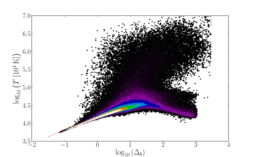
The values of and are measured from the scatter plot (Fig. 1) using only the points with low temperature (). Moreover, all the points that are too overdense () are discarded to take into account only the region of the space where the relation can be modeled with a simple adiabatic form (Eq. 1.1). Additionally, the points too underdense () are not used as well, because our simulations do not have enough resolution to properly model the density field in voids. The remaining points are used in a linear regression model to determine the parameters of the temperature-density relation (in a log-log plane).
The different simulations used are summarized in 1.
| Model | thermal history | |||
|---|---|---|---|---|
| L60 | REF+ | |||
| L30 | REF | |||
| L15 | REF | |||
| L15s | REF |
| Model | descr. | ||
|---|---|---|---|
| REF | Ref | ||
| COLD | Cold | ||
| HOT | Hot | ||
| LG | Low | ||
| HG | High | ||
| HHG | Hot + High | ||
| HLG | Hot + Low | ||
| CHG | Cold + High | ||
| CLG | Cold + Low |
We extract a number of randomly determined lines-of-sight (LOSs) through the simulation box at a given redshift and interpolate the gas properties (density, temperature and velocity) along them. This enables us to determine the optical depth () for each pixel, and in turn the observed flux (). The interpolation scheme adopted in this paper is described in more detail in [43]. The number of pixels along each LOS is chosen to be . The results are robust to this choice (up to a high value for the wavenumber of the recovered power spectrum, which is enough for the purposes of this paper). The number of LOSs is and we have tested that the numbers above are high enough for the statistical estimators to converge.
Once the optical depths due to both Lyman- and Lyman- absorption along all LOSs have been determined, we first re-scale the Lyman- optical depth so that the mean observed flux matches observations at a given redshift. In practice, we rely on the mean flux level measurement inferred from high-resolution spectra presented in [44] which is usually casted in the form of an effective optical depth: . The re-scaling procedure can be interpreted as scaling of the mean Ultraviolet (UV) background flux and we also re-scale optical depth for Lyman- absorption by the same amount. We are allowed this freedom because the relation between mean observed flux and mean UV flux is degenerate and the first is more stringently constrained by observations [45, 46]. We perform this step regardless of the thermal history used in the simulations, but we caution the reader that the mean observed flux depends also on and . The rescaling typically changes the optical depths by an amount which is of the order of %.
The optical depth skewers (in both Lyman- and Lyman-) are then converted into observed flux fluctuations. Those are transformed in the wave-vector () space using Fast Fourier transformation (FFT) techniques using the freely available FFTW library. In the end, the coefficients of the Fourier transform are squared and averaged over all the LOSs to get an estimate on the (auto) power spectrum. The cross power spectrum is obtained by multiplying coefficients of Lyman- flux with those from Lyman-. Since this analysis is only concerned with the recovering of the power spectra at a given redshift and does not model the redshift evolution along the LOS of optical depth, the recovered cross power spectrum will not have any imaginary part contribution, as suggested by [37].
To estimate the error-bars of power spectra we adopt the bootstrap technique. By using randomly determined weighted sum of the Fourier coefficient contribution from each LOS we average over the weights using bootstrap samples. We show that such a number of samples is enough to achieve converged results for the whole covariance matrix of the -bins of each of the power spectra. However, this technique lacks the ability to add covariance between the estimated power spectra, which is something that is not addressed in the present paper.
3 Modelling Lyman- absorption
To model the Lyman- forest absorption we adopt a standard framework which allows us to extract randomly selected skewers through the simulation box at a given redshift. For each pixel along each LOS we interpolate gas related physical quantities and sum over all the contributing gas particles that affect the result within the window function used, thereby relying on a Smoothed Particle Hydrodynamics (SPH) scheme to obtain physical quantities at each pixel. The formalism used is described in more detail in [43]. We consider both the full Voigt profile model of each absorption feature as well as correct for peculiar velocities of the gas along the line-of-sight. The same technique has been used multiple times in many different analysis investigating the Lyman- forest flux statistics like flux probability distribution function, flux power and bispectrum etc. (e.g. [7, 47, 30]).
However, in order to take Lyman- absorption into account as well, we extend the model above. We assume that the only difference between Lyman- and Lyman- absorption comes from different absorption cross sections (main effect) and different natural widths of Lorentz profiles of those two transitions (secondary effect). This implies that the Lyman- and Lyman- optical depths are related as:
| (3.1) |
where the function is a general function of optical depth describing all the physics due to fluctuating density field, gas properties and modelling of the line profiles. By changing the oscillator strength , rest-frame wavelength of the transition () and the natural width we can use the same formalism for Lyman- and for Lyman-.
The values of the atomic physics constants used in our calculations were (as extracted from VPFIT 111Version 10.0 by R.F. Carswell and J.K. Webb, http://www.ast.cam.ac.uk/rfc/vpfit.html: HI-Ly (Å, , ) and HI-Ly (Å, , ).
4 Results
In this section we present our main results. The power spectra obtained from the simulation at redshift are shown in Fig. 2. Although it is clear that on large scales () the three power spectra are in a regime of a constant bias with respect to each other, the small scales highlight the trends of non-linearity due to the transformation.
If the contribution of the different Lorentzian natural widths of the respective lines are neglected, then the relation between and is linear, whereas the relation between the observed fluxes and is not linear on small scales. The observed trend of and getting closer with higher is a result also obtained from N-body simulations using dark matter only [36] and can be interpreted as a result of the non linear nature of the transformation. On sufficiently small scales, the power spectra and grow in a very similar way indicating that both power spectra are tracing the same underlying line structure. Eventually, this behaviour breaks down at even smaller scales where the effect of different natural broadening of the lines comes into play.
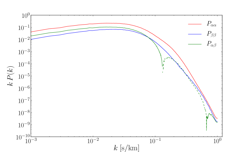
Another very interesting feature to notice is that at small scales (, corresponding to roughly ) the cross power spectrum () crosses zero. In fact, Fig. 3 shows that the cross power spectrum exhibits an oscillation pattern. The normalized cross power spectrum, as plotted in Fig. 3, measures the cross-correlation coefficient which is defined as: 222This is exactly true in the absence of the imaginary part of the cross power spectrum .
| (4.1) |
From the definition above, we see that the cross-correlation coefficient takes strictly positive values. However, in our estimate we choose to preserve the sign of the to stress the features of the oscillatory pattern. Since both and are positive in our measurements (by definition) the transformation of the plot in Fig. 3 to is easily achieved.
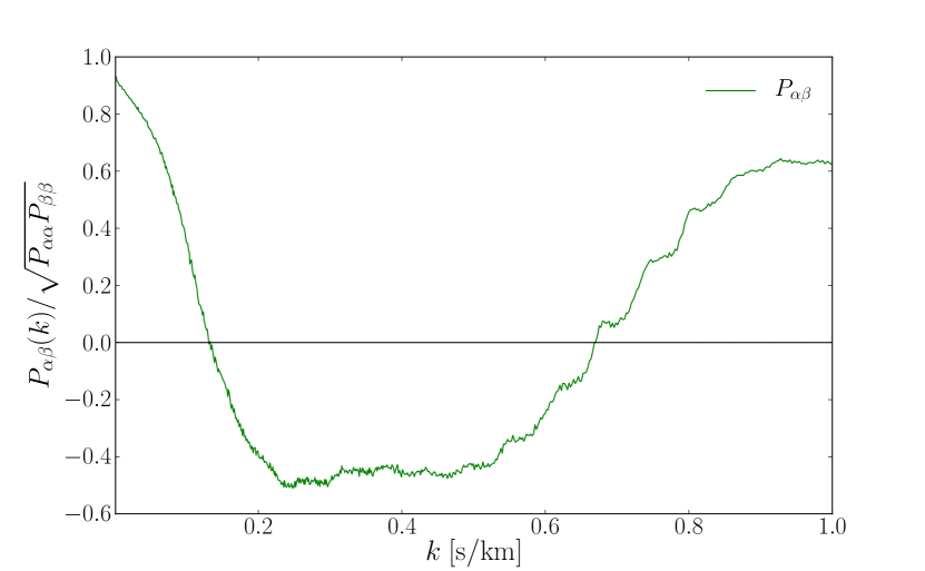
Using the hydrodynamic simulations we confirm the findings that the cross-correlation coefficient goes towards at large scales and falls off at smaller scales, as was measured in BOSS DR9 by [37]. However, we also note that on small scales the cross-correlation coefficient does not go to zero, but rather exhibits an oscillation.
While the details of the oscillations in vary among simulations with different thermal histories, the overall trend remains the same. Since we also note that the oscillation is only weakly damped, we conclude that its nature is due to the non-linearity of the transformation between the density field and the observed flux, rather than carrying physical meaning. However, we caution the reader that the results of this paper are not conclusive on the point of the nature of oscillatory pattern. Further investigation is required to confirm the interpretation given.
Another oscillatory pattern can be seen for in Fig. 3 albeit with a much smaller amplitude and scale, showing up at the smallest of scales () even in . However, this paper is focused on larger scales () and trends could be due to the cross correlation of individual lines that is not the subject of the present investigation.
4.1 The resolution and convergence tests
To test the stability and convergence due to simulation resolution on small scales we have performed additional flux power spectra analysis on two higher resolution simulations: box size with gas and dark matter particles (L30) and box size with the same number of particles (L15). The details of the simulations are summarized in table 1. The higher resolution simulations (L30 and L15) have the same cosmological parameters as used in the L60 simulation suite. However, only the reference (REF) thermal history was considered for the reasons that will be described shortly.
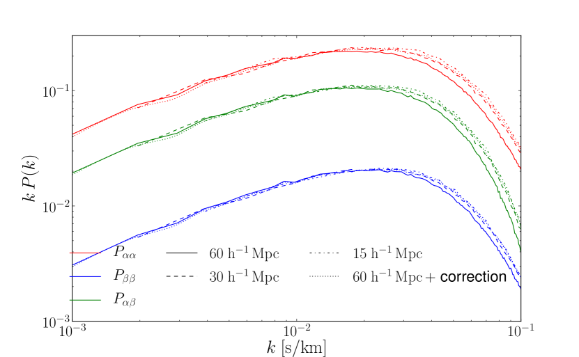
Figure 4 shows the result of changing the resolution of the entire simulation, by keeping the number of both gas and dark matter particles fixed and decreasing the size of the simulated box. As has been noted by other similar resolution tests ([48, 49, 50]) the effect of increasing resolution is the increase of power on small scales, while the large scales remain mostly intact. However, if the resolution would have been decreased further by increasing the size of the box beyond , having fixed the number of particles, an effect on large scales would be seen as well. It is also clear that the convergence of power is reached somewhere between the resolution of L30 and L15, since the curves do not differ from one another. Thus, we can assume that on small scales () the resolution of L15 is good enough to capture the physics of the Lyman- (and Lyman-) forest.
In principle one could correct for this effect using suit of 3 simulations: large box size (but lower resolution) one, and two small box size simulations. Of the two small box size simulations one would have the same number of particles as the large box size simulation (and thus higher resolution) and the other would have the same resolution as the original large box size simulation. Such a correction was first proposed in [48] and is described in more detail therein.
The result of the corrected flux power spectrum for the resolution is shown in Fig. 4 with dotted line. We have only corrected for large-scale normalization and intermediate scales, but not for the low scales where L60 does not sample the power correctly anymore, since our focus in this work is on larger scales. The correction works reasonably well.
It is believed that at first order this kind of correction is independent of the thermal history of the gas in simulations, thus only one (reference) thermal history case needs to be explored to calibrate the correction relations. This might not be entirely true at very high precision on small scales, but we have not explored this issue further.
However, since our final tests and results are obtained on the ratios of flux power spectra between different thermal history simulations and the reference one, any such (thermal history independent) correction for resolution would cancel out completely. This is one of the advantages in working with ratios and was one of the reasons we have chosen such an approach.
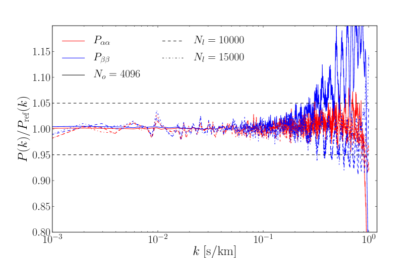
We tested the sensitivity of the power spectra to the changes of parameters of the analysis process, namely the number of LOSs (), over which the flux power spectrum is averaged and the number of pixel bins along each line of sight . Figure 5 shows that on larger scales () the power spectra have converged and the remaining differences are below a few percent level. At small scales, however, the differences grow significantly.
Increasing the resolution along each LOS allows to widen the range at which the power spectra can be measured. As it can be seen in Fig. 5, a larger number of pixel bins along the LOS leads to higher values of at the very small scales (), while remains largely unchanged. This indicates that at those scales and grow even further together than estimated from Fig. 2, further reassuring the point that on those scales the power spectrum traces correlations among individual lines and that the power spectra should be very similar in shape.
4.2 Auto power spectra dependence on the IGM thermal state
We now quantify the dependence of the power spectra , on the parameters of the equation of state (), governing the thermal history of the universe.
To address this issue we analyze the models of Table 1. All the power spectra retrieved from simulations show a general tendency: a change in the thermal history (either temperature or the adiabatic index) changes the scale of an exponential cut-off on the smaller scales, while modifications at the large scales are less pronounced. Of course, the cut-off is not exactly exponential and there are many features introduced in the slope. Also note that at least on small scales there is a visible degeneracy between increasing the temperature of the IGM and lowering the adiabatic index, with different power spectra being sensitive to this change in a different way.
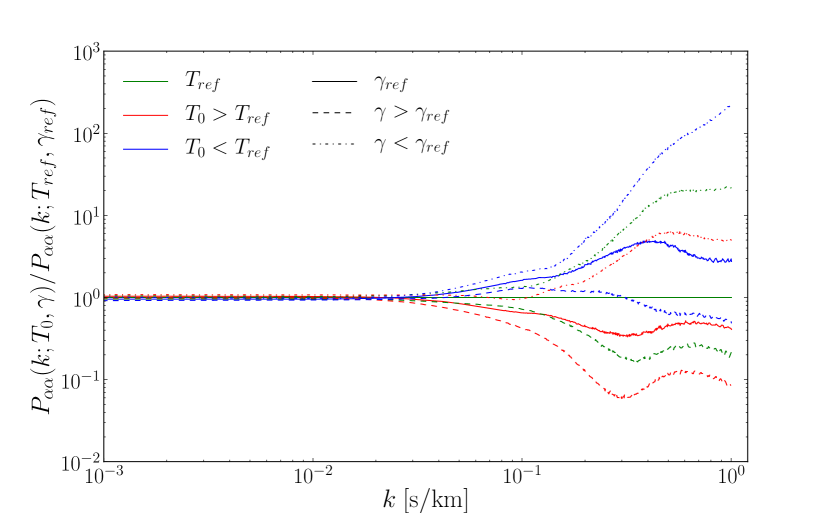
The Lyman- power spectrum, shown in Fig. 6, offers the general indications summed up in the previous paragraphs. While the (relative) changes due to different thermal histories are small on large scales (), they are much more pronounced on small scales. Different colours on the plot show different temperatures of the IGM (green for reference temperature of , blue for colder and red for hotter IGM) and different line styles represent different values of the adiabatic index (full line for reference value of , dashed line for higher values and dash-dotted for lower values of the adiabatic index). As noticed there is a slight degeneracy between varying or , separately, e.g. a hot IGM with adiabatic index closer to (red dash-dotted line) would produce similar results as a cold IGM with reference adiabatic index (blue line). However, both high temperature and high values of the adiabatic index determine a deficit of power on small scales (). The trends found for are similar to those found by [10, 32].
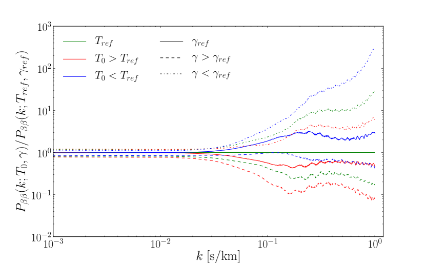
As with Lyman- power spectrum, similar features can be observed when looking at the estimate of the Lyman- power spectrum, shown in Fig. 8 (colours and line styles are the same as in Fig. 6). On small scales we can observe the tendency for both high temperature and high value of to lower the power spectrum, while cold IGM and low value of the adiabatic index increase the power on small scales, when compared to the reference model. However, there is a noticeable difference between Lyman- and Lyman- on large scales (): a regime where the difference between different values of parameters of the equation of state is more pronounced. In fact, there is a clear separation with the value of the adiabatic index: high values of decrease the power, while small values of increase the power on large scales. Whereas the results still remain mostly insensitive (at large scales) to the changes of IGM temperature. This result can be interpreted as follows: a small value of the Lyman- cross section results in a high sensitivity to large values of density of the IGM. Even when Lyman- would produce a near saturation for a high enough density (at a given parameters of equation of state), Lyman- would remain in the regime where the transformation between flux and optical depth remains mostly linear.
We can illustrate this point with a simple toy model. Let us assume that the estimate of the observed flux () is the following tracer of the underlying baryon density field fluctuations ():
| (4.2) |
with constants and . The amplitude constant plays a role of a product of cross section of the line observed and the average temperature of the IGM, thus . On the other hand, the power-law coefficient is related to the adiabatic index . The toy model uses only local optical depth, whereas a correct model should then be convolved with a (Voigt) line profile and corrected for redshift space distortions along the line of sight. However, for our purposes this simple toy model will suffice, since convolution will smear the effects described over large number of scales and redshift space distortions will introduce an additional cutoff scale in the power spectrum that is dependent mostly on cosmological parameters.
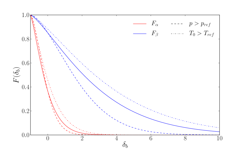
In the toy model described, the only difference between Lyman- and Lyman- flux estimation will be the value of . For any given the ratio of the values of the parameter between Lyman- and Lyman- will be the same and equal to the ratio of cross sections of the absorption lines. Fig. 7 shows the dependence of the observed flux on the underlying baryon density field (). For given reference values of the toy model parameters and , the plot shows that Lyman- flux covers a wider range of densities than the Lyman- model thus allowing to be more sensitive to the factor . We can also interpret this as if, for a given density level threshold, the Lyman- flux is largely insensitive to the changes in density, while for the same threshold Lyman- is still in a relatively mildly non-linear regime of sensitivity. The dashed line demonstrates that changes of the parameter in the toy model have stronger effects on the shape of the Lyman- flux dependence, suggesting that the model is sensitive to even the small changes of in Lyman- flux while not being sensitive in Lyman- flux. On the other hand, changing the value of will shift both flux dependencies in a similar fashion, indicating that both fluxes would be equally sensitive to the change in . Thus, using the simple arguments above, it is clear that Lyman- flux probes higher densities than Lyman- flux due to the fact that lower cross section allows for higher sensitivity in the same range of densities as are probed by Lyman- flux. This would explain why the observed Lyman- power spectrum (see Fig. 8) is more sensitive to the value of the adiabatic index .
Additionally, in Fig. 8 an oscillatory pattern can be seen on very small scales of and is very similar in nature than pattern noticed in . The results indicate that the oscillation pattern is more pronounced for hot gas and low adiabatic index. However, this paper is focused on the dependence of the power spectra on large scales () and we decide not to investigate further the nature of this oscillations.
4.3 The cross spectrum dependence on IGM thermal state
In addition to both the and power spectra we have also investigated the dependence of on the thermal history. While the general statements described so far hold for the cross power spectrum as well and will be more thoroughly discussed in the following, we would like to focus on some very peculiar aspects of the cross power spectrum.
Figure 9 shows the dependence of the normalized cross power spectrum for different combinations of the parameters . An important feature to notice is that the normalized is very insensitive to any change in the thermal history on large scales: this fact has the profound implications that it must depend on cosmological parameters only. Thus, the normalized could become a powerful tool to constrain cosmological models independently of the parameters of the IGM on large scales and should be thus considered in any future Lyman- forest focused on constraining cosmological parameters.
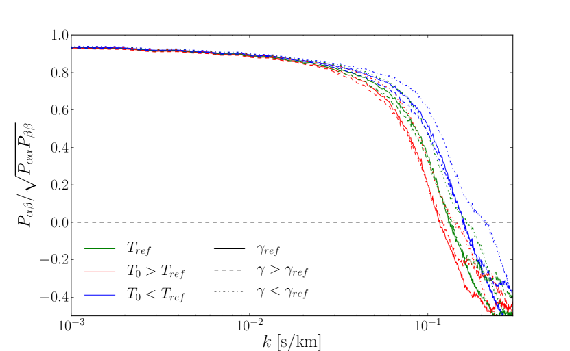
Another important feature in Fig. 9 is the zero-crossing of . We can see that for intermediate and high values of the adiabatic index the zero-crossing is determined only by the temperature of the IGM, while this conclusion is somewhat loosened for low values of the adiabatic index. Estimating the value of independently of the adiabatic index would be very important for understanding the properties of the IGM as well as constraining the parameter space and allowing for better estimates of the cosmological parameters. However, we caution the reader that the scales of zero-crossing ( are on the boundary of scales that are confidently retrieved from the current measurements.
Any future Lyman- surveys with high resolution and signal-to-noise ratio could use this unique feature of the to significantly improve current constraints on , since neither Lyman- nor Lyman- can constrain alone to high precision. High resolution would allow us to push to smaller scales and confidently measure the scales where the crossing occurs. We stress however that the high signal-to-noise ratio and a very precise understanding of the instruments noise is crucial to determine the zero-crossing. This is because without the precise knowledge of noise properties zero-crossing becomes crossing of an arbitrary threshold value of the power spectrum. However, Fig. 9 shows that is sensitive to and insensitive to only in a small range around the scales where the cross-power spectrum changes sign. This high sensitivity of the cross-spectrum to only would be weaker at other scales.
4.4 A closer look to the power spectra: quantitative dependence on IGM thermal state
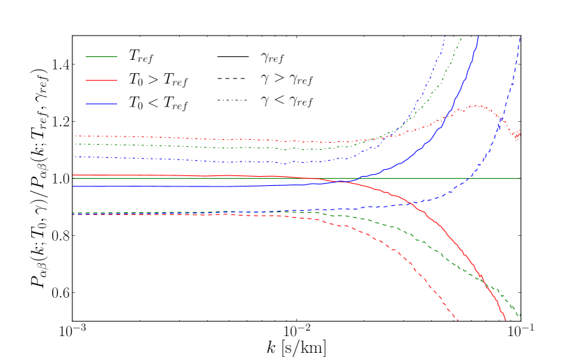
Here, we decide to have a closer look at the large scales. The scale dependence of the three power spectra in the range of is shown in the following figures (Fig. 10, 11 and 12). They are a zoom-ed in versions of the figures (Fig. 6, 8 and 9), focussing on the larger scales of the retrieved power spectra (). All three power spectra grow constant relative to the reference model, indicating that on large scales (), each of the power spectrum has the same shape, but a different amplitude, that varies with thermal history.
On the largest scales of , shown in Fig. 10, it is the colder gas that produces deficit of power, whereas on small scales colder gas produced an excess of power when compared to the reference model. This shows that the average temperature of the gas affects the flux power spectrum differently on different scales, and comes in with a strong scale dependence that also changes the sign (compared to the reference value). Comparing Fig. 6 and 10 for Lyman- flux power spectrum, it is possible to write down approximate scaling relations for the temperature and the adiabatic index.
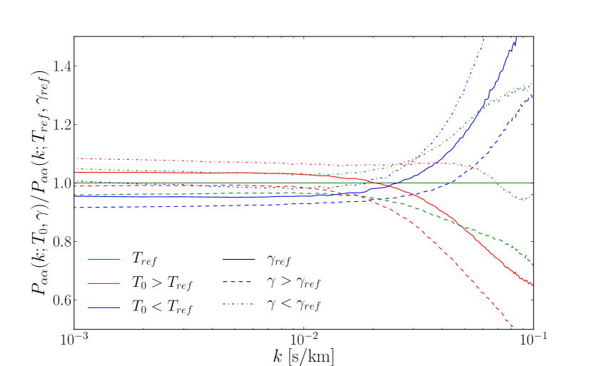
The can be thought of as a function of scale with additional parameters and . If one would expand into a Taylor series over the parameter space around some reference model, the linear contribution could be written as:
| (4.3) |
The above equation allows us to provide a mathematical context for unveiling the relation between power spectra and thermal parameters. Since the first partial derivatives over parameters depend only on scale and reference values (but not on the actual values of the parameters), one can easily interpret the scalings seen in Fig. 10. By keeping the adiabatic index fixed at the reference value, the only dependence will come from linear Taylor term in the temperature. As already discussed (Fig. 10), at large scales higher temperature produce excess of power while on smaller scales it is reverse. The pivot scale around where the behaviour changes is around . We can thus approximate the first derivative term with respect to temperature as:
| (4.4) |
where the first term, the power spectrum at the reference value, comes from the fact that the ratio of power spectra is plotted in Fig. 10. If the amplitude () of the temperature derivative term and the pivot scale () are chosen to best reproduce the simulations we get and . We caution the reader that these values were not produced in a fit of any sort, nor was the specific scale dependence chosen to best match the simulations. Both the parameter values and the function are just an illustration in this case. However, they work reasonably well in determining the general behaviour of the dependence of on and are very simple in form.
In a similar fashion to the first derivative with respect to temperature, we can also model the dependence. Fixing the temperature of the gas to the reference value, it is clear from Fig. 10 that changing the adiabatic index either only increases or only decreases power on all scales. Inspired by the result of Eq. 4.4, we can write the first derivative with respect to the adiabatic index as:
| (4.5) |
where the values of and are the same as in the temperature dependent term in Eq. 4.4.
From both the toy models and the results shown in Fig. 10 one can see that Lyman- flux power spectrum does not distinguish well between different models of thermal history, especially at large scales. The difference is at most and there is a strong degeneracy between the temperature and the adiabatic index.
Combining Eqns. 4.4 and 4.5 and rearranging the terms to collect those with the same power of , one can show that in the linear model the parameters combination is most sensitive to the quantity . This further supports the argument of the strong degeneracy between the two parameters.
On the other hand, the Lyman- flux power spectrum is much more sensitive to thermal history than Lyman-, as shown in Fig. 11. From the figure it is clear that is very sensitive to the change in adiabatic index on large scales, whereas there is no clear improvement in the change of compared to Lyman- flux power spectrum.
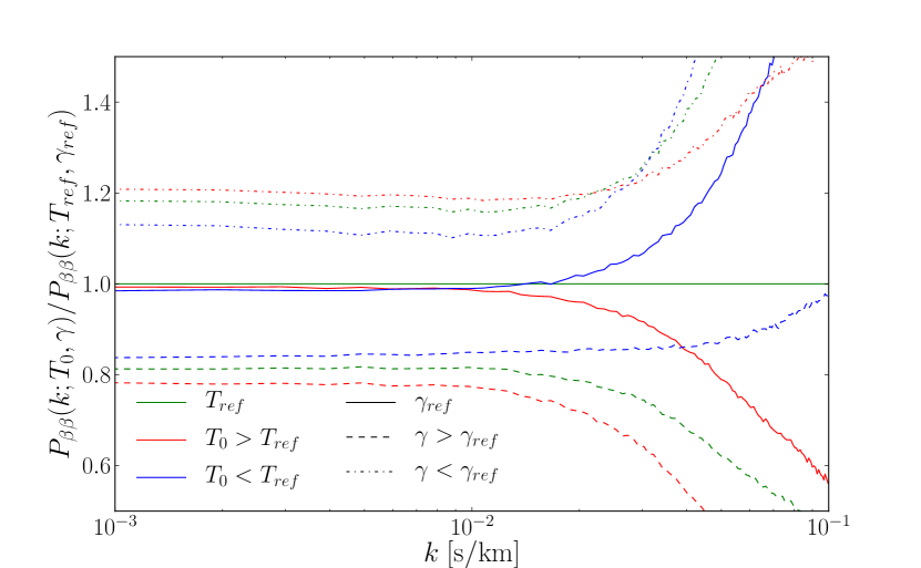
A Taylor expansion over the parameters of the equation of state can be made for as well. Similarly to Eqns. 4.4 and 4.5 we can write an approximate model, to underline the general behaviour observed in simulations as:
| (4.6) |
where the amplitude and pivot scale can be chosen to have the same values as the ones describing . Thus putting and will ensure that the approximation works reasonably well when it comes to predicting the general behaviour. However one can quickly see the limitations of the above equation. Firstly, it is very clear from Fig. 11 that the curves representing COLD and HOT model or LG and HG model are not symmetric around the reference model, thus a simple linear dependence will not be sufficient to capture this trend. Secondly, the above toy model (4.6) would indicate that on large scales there is no difference in models with different average temperature of the IGM. While this is roughly true for reference model, adding shows small albeit distinct separation thus suggesting that either the temperature term has a weak constant term in addition to the quadratic term in , or that there is a non-linear term linking and . In fact a cross term that goes as might be closest to the functional form observed in power spectrum. Another important feature to note in Eq. 4.6 is the high value of the constant term in dependence which tries to explain the observed strong separation of models with different adiabatic index.
The fact that Lyman- is more sensitive to the adiabatic index () was already pointed out and is most likely linked to the fact that the nonlinearity of the relation enhances the Lyman- ability to be sensitive to higher densities. If one would perform a parameter estimation analysis based on the simulation results, one would expect a strong constraints on the coming from Lyman- flux power spectrum.
Once again we stress that these equations (Eqns. 4.4, 4.5 and 4.6) are not a fit to the simulations but merely a toy model, showing the general trends of changing temperature and the adiabatic index that we see in simulations. These toy models should not be regarded as tools for parameter estimation studies.
The cross power spectrum shows similar behaviour on large scales as and . As in Fig. 12, the cross power is sensitive to on large scales, and is between and in the sensitivity regime, a non-symmetric dependence on the temperature. The is sensitive to the temperature at low values of adiabatic index, whereas at high values of , it is nearly completely independent of the temperature at large scales (). Note that in Fig. 12 we are plotting for different thermal histories divided by the reference model, unlike in Fig. 9 where we plotted a normalized cross power spectrum. While normalized offers a wide variety of possible tools to determine the cosmology or the physics of IGM, in the rest of this paper we focus on using the not normalized and its information on the large scales. As Fig. 12 might indicate, the constraints coming from on will be similar to those of , while nothing can be concluded about the constraints on the .
4.5 Adding signal-to-noise ratio and resolution effects
So far we have shown that all three power spectra have very interesting and potentially powerful features at both large and small scales that would help put tighter constraints on the equation of state parameters and thus allow for better estimation of the cosmological parameters.
However, the current instruments with medium or low resolution and reasonable signal-to-noise ratio would undoubtedly set a limit on the amount of information that could be retrieved. We proceed by estimating the highest -mode that current surveys would still be able to reproduce without being contaminated by either imperfect knowledge of the instrument resolution and/or noise.
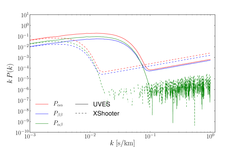
Fig. 13 shows the three power spectra (, and ) retrieved from post-processed skewers through simulation box. The thermal history model used was the reference one. The post-processing involved adding the specific noise model and convolving with resolution of real experiments. Each flux LOS has been convolved with a Gaussian profile of a given FWHM to mimic the effect of finite resolution of the spectrograph. Furthermore, a randomly generated Gaussian noise was added to the flux along each line of sight. The noise was divided into a flux independent part and a flux dependent part that is present in any higher resolution survey. The Fig. 13 shows power spectra (full line) retrieved from a high resolution spectrograph (such as UVES data as processed in [6]) with FWHM and noise model with flux dependent signal-to-noise ratio of and flux independent ratio of . The dashed line shows power spectra as they would have been retrieved from a medium resolution and signal-to-noise experiment such as X-Shooter [51]. The values chosen are conservative for that experiment with FWHM and .
As we can see from the Fig. 13, adding realistic noise properties to the flux from simulations and not accounting for it in the subsequent analysis of the flux makes it hard to observe small scale power. Moreover, the addition of resolution effects introduces a cut-off around the scales of . This is the scale where the zero-crossing of occurs as well as most non-linearities in the and . In a realistic experiment, both effects will be modeled and removed but this plot shows where the effects will take place if the properties of the noise or resolution are not known to a high precision or removed correctly. Thus, for any future surveys willing to measure the properties of the power spectra introduced in this paper it will be of the utmost importance to know and model the noise and resolution of the spectrograph.
In the case where the resolution is known and removed correctly the limiting factor is the noise of the data. The noise starts to become important around the scales of , and a careful modelling is required to reproduce the power spectrum at the small scales because the perturbations giving rise to power on those scales are much smaller than the noise power. Due to this limiting factor of real data sets and the fact that current experiments extend only to around the aforementioned scales we have decided to carefully model and examine only scales up to . Another important factor in this decision is also the fact that modelling at smaller scales is increasingly harder due to much more pronounced non-linearities and also feedback/astrophysical effects might come into play [10, 16].
4.6 Empirical fit to the power spectra
We have illustrated the general features of the power spectra dependence relative to some fixed reference model of thermal history in the previous sections. However, those were toy models barely illustrating the general parameter dependence and not proper fits to the simulations.
To investigate the parameter dependence of the power spectra we have adopted a full fitting function, following Eq. 4.3. The fitting function was based relatively to the reference thermal history model REF (see Table 1). The power spectrum as a function of the mode with arbitrary parameters is thus:
| (4.7) |
where the index runs over all the possible power spectra, i.e. . The fitting function as a function of was chosen to be a polynomial of order 3:
| (4.8) |
where the pivot scale was chosen to be and was fixed in the fitting procedure. All the coefficients for each of the power spectra are a linear combination of the thermal history parameters . This can be summarized as:
| (4.9) |
where is the average temperature of the gas in the units of . The terms of Eqns. 4.7, 4.8 and 4.9 can be rearranged into ones similar to those of a Taylor series expansion given in Eq. 4.3 to see that in the fitting function adopted in this paper we have extended the Taylor series expansion to second order in parameters of the temperature-density relation. The above prescription is based on the simple toy models where we have seen that expansion to linear order in and quadratic functions in describe the general behaviour well. However, this form was not motivated by any physical processes and there might be a better functional form able to more fully capture the non-linear behaviour of the power spectra.
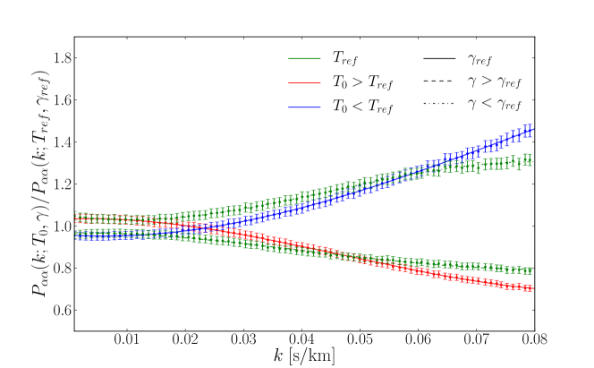
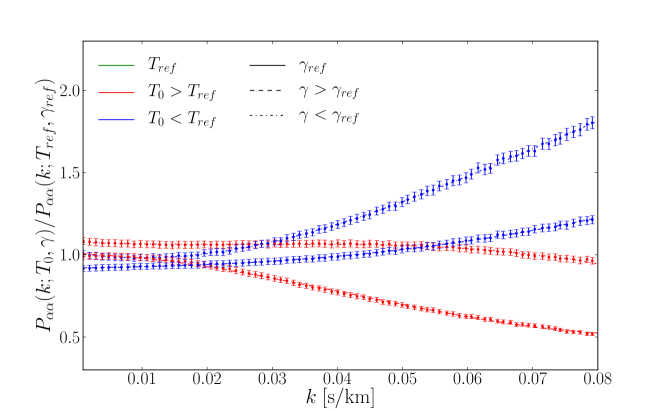
A relatively simple form of the fitting function with parameters for each power spectrum is enough to describe the relative changes to the power spectra due to the equation-of-state parameters. In this fit, all the other parameters a power spectrum might depend on, were fixed (such as cosmological parameters, etc.). The range of modes over which the fitting function works very well and where we have decided to fit for the exact values of the parameters is for .
While in principle we believe it is possible to use the same fitting function to extend to larger scales it is not possible to use it on smaller scales. The nonlinearities induced by both the nonlinear transformation between the flux and the density field, as well as non-trivial and highly-nonlinear dependence on the thermal history of the power spectrum on small scales render this approach impractical and incorrect on small scales. However, since most of the recent experiments measure power spectra reliably only up to it seems sufficient to use that range to show what an improvement an inclusion of the Lyman- power spectrum can bring to the estimation of the equation-of-state parameters.
Another possibility of an empirical fitting formula with a few more parameters was proposed by [48]. While this method is capable of fitting the power spectrum directly and is not aimed at capturing the ratios between different thermal histories it requires a good estimation of large scales to properly fix all of the model parameters. However in this work, we have adopted a new, simpler empirical fit, aimed only at describing the thermal history dependence of the flux power spectra.
Figure 14 shows the results of the fitting procedure for for all the different thermal histories. It is clear that the relatively simple fitting function is able to describe the changes of the power spectrum due to different thermal histories. The fit is performing well on large scales and starts to get worse on small scales, as expected since on small scales non-linearities dominate and are not captured in the fitting function. To account for the variability of the power spectrum, due to different thermal histories, a further study is necessary. Also the fit seems to perform better for different values of average gas temperature while changing produces largest discrepancies on small scales, especially when coupled with high gas temperatures.
The error bars shown in the Fig. 14 are estimated using bootstrap method on the extracted LOSs through the simulation box. Only diagonal elements of the bootstrap matrix were used in the chi-square estimation of the parameters. Inclusion of the correlations between the different -bins would only change the errors on the parameters slightly but would not change their mean value.
Overall, the estimated parameters given along with the reference thermal history model (REF) provides a very good description of the three power spectra (,,) in the wavenumber range of . The fitted numbers for the parameters are given in Appendix: The values of the fitted parameters.
5 Fisher matrix analysis
Using the empirical fit presented in the previous section we perform the Fisher matrix analysis on the parameters of the equation-of-state. The Fisher matrix analysis is widely used to forecast the precision of an experiment. In our case we will use the Fisher matrix to forecast the precision with which the equation of state parameters (,) would be extracted from the simulations using both Lyman- and Lyman- forests.
In this paper we assume simulations are our experiments in the sense that the former will predict real data observations of the flux power spectra. Our analysis makes two assumptions about bootstrap errors on the simulations: we do not take into account the full covariance matrix of the bootstrap sampling but only the diagonal elements (which we call bootstrap errors); and we further assume that the bootstrap errors on the simulations would trace errors on the flux power spectrum from the real data. At this stage we do not take into account the effects of real data noise and improper beam corrections because to properly account for those two effects an analysis should be run on a full mock data.
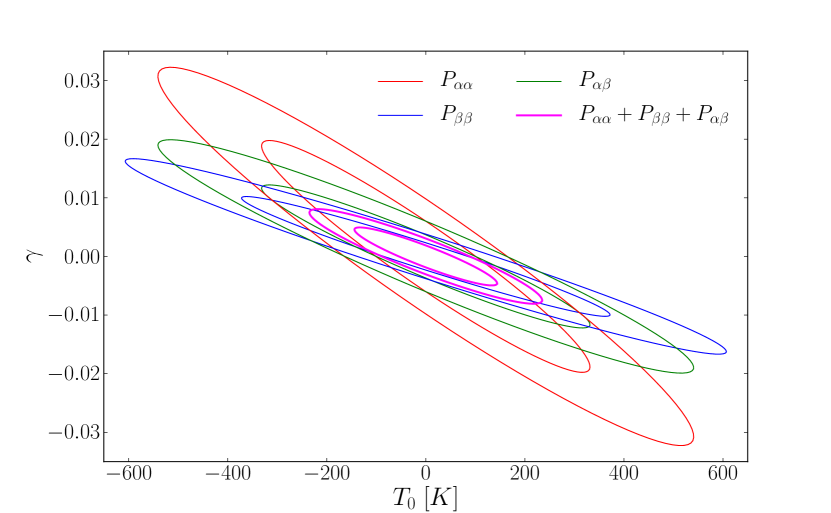
Figure 15 summarizes the main result of this paper and displays the 1 and 2 contours in the plane of the “equation-of-state” parameters and . The contours are centered around the reference mean value points (REF model). Different colours represent contours obtained from different power spectra or when combining all the power spectra. From Fig. 15 it is clear that there is big () improvement to the constraints on coming from Lyman- compared to the ones from Lyman- flux power spectrum. It is important to note is that the Lyman- flux power spectrum constraints the parameters space of equation of state in a different way than Lyman- flux power, and the figure is quantifying this. The constraints from the real part of the cross power spectrum are similar to those from Lyman- yet slightly less stringent. However, they add important independent information so when combining the information for all three flux power spectra the constraints on both and can be tightened considerably (by on ) compared to just using Lyman- flux power.
The Fig. 15 also shows very clearly the degeneracies between and as indicated in Sec. 4.4. The plot nicely shows that and are strongly (anti-)correlated in the case of the Lyman- power spectrum, while this degeneracy is slightly lifted in using Lyman- power spectrum.
Note that in this paper we have performed all the analysis assuming equal effective path length for both the Lyman- and Lyman- optical depth sight-lines. However, in any real data, the Lyman- forest path length would be roughly 20 the path length of Lyman- forest, which would result in roughly a factor of improvement in the errorbars on and from Lyman- alone.
6 Conclusions
The interest in measuring the IGM thermal state is twofold: on one side it is of primary importance to constrain the IGM thermal state in order to lower the impact that such nuisance parameters have in terms of cosmological derived parameters; on the other side, measuring the IGM thermal state can shed light on the IGM/galaxy interplay and on the overall evolution of baryons helping to understand aspects like feedback and Helium or Hydrogen reionization. Moving from Lyman- to Lyman- forest and relying on different flux statistics (e.g. flux probability distribution function, bispectrum, curvature of the transmitted flux, etc.) for both the transitions can be a very promising technique.
It has been first suggested in [36] that using Lyman- power spectrum one could improve the constraints on the IGM parameters (e.g. parameters of the relation). Also following the recent measurements of the Lyman- power spectrum [37] we have performed a more detailed study of Lyman- forest constraints on the IGM parameters.
Using a suite of high resolution hydrodynamic simulations, we have investigated how the Lyman- and Lyman- flux power spectra change in the presence of different thermal histories. We have also included the (real part of the) cross power spectrum in the calculations.
The main findings of this paper can be summarized as follows.
-
(i)
For a given thermal history all three power spectra , and show constant bias among each other on large scales (). If (and ) are biased tracers of (and thus of the underlying matter distribution) then the bias on large scales would depend only on the different sensitivity of the and to the IGM thermal parameters.
-
(ii)
The real part of the cross power spectrum displays a distinct oscillation pattern at small scales (). The oscillation pattern is such that crosses zero and becomes negative at a specific range of scales.
-
(iii)
The normalized cross power is insensitive to thermal history on large scales (). Furthermore, the crossing of zero is sensitive only to at high and intermediate values of . However, this specific property is only true on a small scale range around the (first) crossing of zero ().
-
(iv)
The dependence of on thermal history is much more pronounced than for . As explained in the paper we believe this is because the Lyman- absorption probes denser regions due to smaller optical depth of the Lyman- absorption cross-section. This is most simply seen in the fact that is very sensitive to different values , suggesting that the values of the overdensities probed are typically larger than the corresponding ones probed in .
-
(v)
Using the Fisher matrix formalism we show that the alone is more sensitive to than , putting times more stringent constraints on that IGM parameter. Combining the information from all three power spectra improves the estimation compared to using only even further to achieve times tighter constraints on the slope of the relation and times tighter constraints on the mean average temperature.
While in this paper we show that is more sensitive to thermal IGM parameters, particularly the slope of the temperature-density relation, our analysis has still to be intended as preliminary. For example, in our analysis we have fixed the cosmology to the cosmic microwave background values, so it is not clear by which amount the could improve the constraints on the cosmological parameters. This is of course of much interest and further analysis should be conducted to investigate the joint parameter space. Moreover, our empirical fit is parametrized only by parameters of the relation and thus does not take into account the damping due to Jeans filtering which is a more complicated (integrated) function of the thermal history of the universe. Finally, our assumption is that the relation can be described by a simple power-law relation and this can break down around HeliumII reionization (e.g. [52, 19]). It will be also important to test the full procedure on top of more refined mock quasar spectra that incorporate all the relevant instrumental effects in a similar way as it is presently done in the BOSS collaboration (see e.g. [53]).
An interesting point that we have not further investigated in this paper is the effect of the scatter in the relationship on the final result. Much like the flux power spectrum, temperature-density relation is another important analysis tool that can be used to characterize the physics of the IGM. In this work, however, we have only used the scatter plot in a regime where the power-law approximation is valid, and the scatter is small. The values of the parameters extracted in this way are then used as a parameterization of the flux power spectrum (for both Lyman- and Lyman-). One might worry that since Lyman- flux power spectrum is more sensitive to higher density regions, it would be more affected by the scatter in the relationship. However, the analysis presented in this paper does not aim at constraining the temperature-density relation, but only a possible parameterization of it. The results of the fitting functions and Fisher matrix analysis are in that sense completely independent of scatter. Nevertheless, one might construct a different approximation of the relationship, going beyond the simple power law approximation (e.g. stochastic or asymmetric scatter or density dependent scatter). In such a case one could parameterize the relation with more than just and and possibly, by using both Lyman- and Lyman- flux power spectrum, it might put some constraints of the scatter of the underlying IGM relation. The scatter would then act as an additional parameter (or parameters if the scatter model was complex) that could be used to expand the flux power spectrum around the reference model. It is definitely an interesting possibility that would allow us to probe even more complex approximations of the relation, using the Lyman- and Lyman- power spectrum.
Also we have not investigated the special properties of the cross power spectrum at relatively small scales. The offers a unique probe of the temperature of the IGM but the relation of the zero crossing needs to be investigated further, for example by varying cosmological parameters as well. More work is thus required to investigate the issues presented here and to fully exploit extremely promising potential of the Lyman- forest in measuring the properties of the IGM and in constraining cosmological parameters.
Acknowledgments
We thank Jamie Bolton for having provided the thermal histories routine used in the present paper and for useful discussions. MV is supported by the ERC Starting Grant “CosmoIGM” and by the IS PD51 INDARK INFN grant.
Appendix: The values of the fitted parameters
The parameter values obtained from a fit to power spectrum are:
| (A1) |
where the parameter errors quoted are the 1- errorbars. We can see that all parameters are estimated with relatively high significance. However, the temperature dependence of the parameter seems to be poorly estimated, indicating that the does not depend on the or that its dependence on does not change the final chi-square much.
With the same fitting function we also fitted for power spectrum, obtaining the following parameter values:
| (A2) |
where the errors quoted are again the 1- errors on the parameters. The parameters are also slightly correlated. However the errorbars are much smaller than the bootstrap errors on the power spectrum bins, and thus any estimation of the () parameters using the above empirical fit would be dominated by the errorbars on the power spectrum bins.
The same procedure as for and power spectra was also carried out for the cross power spectrum . The estimated parameter values are:
| (A3) |
where the errorbars are the 1- errors. In the parameter estimation for both and we can see that the temperature dependence of is not well constrained at all, giving further indication that in the region fitted by the empirical function (Eq. 4.8) the parameter in front of the linear -term does not depend on the temperature.
References
- [1] M. Rauch, The Lyman Alpha Forest in the Spectra of QSOs, ARAA 36 (1998) 267–316, [astro-ph/9806286].
- [2] A. A. Meiksin, The physics of the intergalactic medium, Reviews of Modern Physics 81 (Oct., 2009) 1405–1469, [arXiv:0711.3358].
- [3] P. McDonald, J. Miralda-Escudé, M. Rauch, W. L. W. Sargent, T. A. Barlow, R. Cen, and J. P. Ostriker, The Observed Probability Distribution Function, Power Spectrum, and Correlation Function of the Transmitted Flux in the Ly Forest, ApJ 543 (Nov., 2000) 1–23, [astro-ph/9911196].
- [4] M. Zaldarriaga, L. Hui, and M. Tegmark, Constraints from the Ly Forest Power Spectrum, ApJ 557 (Aug., 2001) 519–526, [astro-ph/0011559].
- [5] R. A. C. Croft, D. H. Weinberg, M. Bolte, S. Burles, L. Hernquist, N. Katz, D. Kirkman, and D. Tytler, Toward a Precise Measurement of Matter Clustering: Ly Forest Data at Redshifts 2-4, ApJ 581 (Dec., 2002) 20–52, [astro-ph/0012324].
- [6] T.-S. Kim, M. Viel, M. G. Haehnelt, R. F. Carswell, and S. Cristiani, The power spectrum of the flux distribution in the Lyman forest of a large sample of UVES QSO absorption spectra (LUQAS), MNRAS 347 (Jan., 2004) 355–366, [astro-ph/0308103].
- [7] M. Viel, M. G. Haehnelt, and V. Springel, Inferring the dark matter power spectrum from the Lyman forest in high-resolution QSO absorption spectra, MNRAS 354 (Nov., 2004) 684–694, [astro-ph/0404600].
- [8] P. McDonald, U. Seljak, S. Burles, D. J. Schlegel, D. H. Weinberg, R. Cen, D. Shih, J. Schaye, D. P. Schneider, N. A. Bahcall, J. W. Briggs, J. Brinkmann, R. J. Brunner, M. Fukugita, J. E. Gunn, Ž. Ivezić, S. Kent, R. H. Lupton, and D. E. Vanden Berk, The Ly Forest Power Spectrum from the Sloan Digital Sky Survey, ApJS 163 (Mar., 2006) 80–109, [astro-ph/0405013].
- [9] N. Palanque-Delabrouille, C. Yèche, A. Borde, J.-M. Le Goff, G. Rossi, M. Viel, É. Aubourg, S. Bailey, J. Bautista, M. Blomqvist, A. Bolton, J. S. Bolton, N. G. Busca, B. Carithers, R. A. C. Croft, K. S. Dawson, T. Delubac, A. Font-Ribera, S. Ho, D. Kirkby, K.-G. Lee, D. Margala, J. Miralda-Escudé, D. Muna, A. D. Myers, P. Noterdaeme, I. Pâris, P. Petitjean, M. M. Pieri, J. Rich, E. Rollinde, N. P. Ross, D. J. Schlegel, D. P. Schneider, A. Slosar, and D. H. Weinberg, The one-dimensional Ly forest power spectrum from BOSS, A&A 559 (Nov., 2013) A85, [arXiv:1306.5896].
- [10] P. McDonald, U. Seljak, R. Cen, D. Shih, D. H. Weinberg, S. Burles, D. P. Schneider, D. J. Schlegel, N. A. Bahcall, J. W. Briggs, J. Brinkmann, M. Fukugita, Ž. Ivezić, S. Kent, and D. E. Vanden Berk, The Linear Theory Power Spectrum from the Ly Forest in the Sloan Digital Sky Survey, ApJ 635 (Dec., 2005) 761–783, [astro-ph/0407377].
- [11] U. Seljak, A. Slosar, and P. McDonald, Cosmological parameters from combining the Lyman- forest with CMB, galaxy clustering and SN constraints, JCAP 10 (Oct., 2006) 14, [astro-ph/0604335].
- [12] M. Viel, J. Lesgourgues, M. G. Haehnelt, S. Matarrese, and A. Riotto, Constraining warm dark matter candidates including sterile neutrinos and light gravitinos with WMAP and the Lyman- forest, Phys. Rev. D 71 (Mar., 2005) 063534, [astro-ph/0501562].
- [13] N. G. Busca, T. Delubac, J. Rich, S. Bailey, A. Font-Ribera, D. Kirkby, J.-M. Le Goff, M. M. Pieri, A. Slosar, É. Aubourg, J. E. Bautista, D. Bizyaev, M. Blomqvist, A. S. Bolton, J. Bovy, H. Brewington, A. Borde, J. Brinkmann, B. Carithers, R. A. C. Croft, K. S. Dawson, G. Ebelke, D. J. Eisenstein, J.-C. Hamilton, S. Ho, D. W. Hogg, K. Honscheid, K.-G. Lee, B. Lundgren, E. Malanushenko, V. Malanushenko, D. Margala, C. Maraston, K. Mehta, J. Miralda-Escudé, A. D. Myers, R. C. Nichol, P. Noterdaeme, M. D. Olmstead, D. Oravetz, N. Palanque-Delabrouille, K. Pan, I. Pâris, W. J. Percival, P. Petitjean, N. A. Roe, E. Rollinde, N. P. Ross, G. Rossi, D. J. Schlegel, D. P. Schneider, A. Shelden, E. S. Sheldon, A. Simmons, S. Snedden, J. L. Tinker, M. Viel, B. A. Weaver, D. H. Weinberg, M. White, C. Yèche, and D. G. York, Baryon acoustic oscillations in the Ly forest of BOSS quasars, A&A 552 (Apr., 2013) A96, [arXiv:1211.2616].
- [14] A. Slosar, V. Iršič, D. Kirkby, S. Bailey, N. G. Busca, T. Delubac, J. Rich, É. Aubourg, J. E. Bautista, V. Bhardwaj, M. Blomqvist, A. S. Bolton, J. Bovy, J. Brownstein, B. Carithers, R. A. C. Croft, K. S. Dawson, A. Font-Ribera, J.-M. Le Goff, S. Ho, K. Honscheid, K.-G. Lee, D. Margala, P. McDonald, B. Medolin, J. Miralda-Escudé, A. D. Myers, R. C. Nichol, P. Noterdaeme, N. Palanque-Delabrouille, I. Pâris, P. Petitjean, M. M. Pieri, Y. Piškur, N. A. Roe, N. P. Ross, G. Rossi, D. J. Schlegel, D. P. Schneider, N. Suzuki, E. S. Sheldon, U. Seljak, M. Viel, D. H. Weinberg, and C. Yèche, Measurement of baryon acoustic oscillations in the Lyman- forest fluctuations in BOSS data release 9, JCAP 4 (Apr., 2013) 26, [arXiv:1301.3459].
- [15] P. McDonald, U. Seljak, R. Cen, P. Bode, and J. P. Ostriker, Physical effects on the Ly forest flux power spectrum: damping wings, ionizing radiation fluctuations and galactic winds, MNRAS 360 (July, 2005) 1471–1482, [astro-ph/0407378].
- [16] M. Viel, J. Schaye, and C. M. Booth, The impact of feedback from galaxy formation on the Lyman transmitted flux, MNRAS 429 (Feb., 2013) 1734–1746, [arXiv:1207.6567].
- [17] E. Puchwein, C. Pfrommer, V. Springel, A. E. Broderick, and P. Chang, The Lyman forest in a blazar-heated Universe, MNRAS 423 (June, 2012) 149–164, [arXiv:1107.3837].
- [18] M. Viel, M. G. Haehnelt, R. F. Carswell, and T.-S. Kim, The effect of (strong) discrete absorption systems on the Lyman forest flux power spectrum, MNRAS 349 (Apr., 2004) L33–L37, [astro-ph/0308078].
- [19] M. McQuinn, A. Lidz, M. Zaldarriaga, L. Hernquist, P. F. Hopkins, S. Dutta, and C.-A. Faucher-Giguère, He II Reionization and its Effect on the Intergalactic Medium, ApJ 694 (Apr., 2009) 842–866, [arXiv:0807.2799].
- [20] L. Hui and N. Y. Gnedin, Equation of state of the photoionized intergalactic medium, MNRAS 292 (Nov., 1997) 27, [astro-ph/9612232].
- [21] L. Hui and Z. Haiman, The Thermal Memory of Reionization History, ApJ 596 (Oct., 2003) 9–18, [astro-ph/0302439].
- [22] J. Schaye, T. Theuns, M. Rauch, G. Efstathiou, and W. L. W. Sargent, The thermal history of the intergalactic medium∗, MNRAS 318 (Nov., 2000) 817–826, [astro-ph/9912432].
- [23] M. Ricotti, N. Y. Gnedin, and J. M. Shull, The Evolution of the Effective Equation of State of the Intergalactic Medium, ApJ 534 (May, 2000) 41–56, [astro-ph/9906413].
- [24] G. C. Rudie, C. C. Steidel, and M. Pettini, The Temperature-Density Relation in the Intergalactic Medium at Redshift langzrang = 2.4, ApJL 757 (Oct., 2012) L30, [arXiv:1209.0005].
- [25] J. S. Bolton, G. D. Becker, M. G. Haehnelt, and M. Viel, A consistent determination of the temperature of the intergalactic medium at redshift z = 2.4, MNRAS 438 (Mar., 2014) 2499–2507, [arXiv:1308.4411].
- [26] T. Theuns and S. Zaroubi, A wavelet analysis of the spectra of quasi-stellar objects, MNRAS 317 (Oct., 2000) 989–995, [astro-ph/0002172].
- [27] T. Theuns, S. Zaroubi, T.-S. Kim, P. Tzanavaris, and R. F. Carswell, Temperature fluctuations in the intergalactic medium, MNRAS 332 (May, 2002) 367–382, [astro-ph/0110600].
- [28] A. Lidz, C.-A. Faucher-Giguère, A. Dall’Aglio, M. McQuinn, C. Fechner, M. Zaldarriaga, L. Hernquist, and S. Dutta, A Measurement of Small-scale Structure in the 2.2-4.2 Ly Forest, ApJ 718 (July, 2010) 199–230, [arXiv:0909.5210].
- [29] A. Garzilli, J. S. Bolton, T.-S. Kim, S. Leach, and M. Viel, The intergalactic medium thermal history at redshift z = 1.7-3.2 from the Ly forest: a comparison of measurements using wavelets and the flux distribution, MNRAS 424 (Aug., 2012) 1723–1736, [arXiv:1202.3577].
- [30] J. S. Bolton, M. Viel, T.-S. Kim, M. G. Haehnelt, and R. F. Carswell, Possible evidence for an inverted temperature-density relation in the intergalactic medium from the flux distribution of the Ly forest, MNRAS 386 (May, 2008) 1131–1144, [arXiv:0711.2064].
- [31] K.-G. Lee, J. P. Hennawi, D. N. Spergel, D. H. Weinberg, D. W. Hogg, M. Viel, J. S. Bolton, S. Bailey, M. M. Pieri, W. Carithers, D. J. Schlegel, B. Lundgren, N. Palanque-Delabrouille, N. Suzuki, D. P. Schneider, and C. Yeche, IGM Constraints from the SDSS-III/BOSS DR9 Ly-alpha Forest Flux Probability Distribution Function, ArXiv e-prints (May, 2014) [arXiv:1405.1072].
- [32] M. Viel and M. G. Haehnelt, Cosmological and astrophysical parameters from the Sloan Digital Sky Survey flux power spectrum and hydrodynamical simulations of the Lyman forest, MNRAS 365 (Jan., 2006) 231–244, [astro-ph/0508177].
- [33] G. D. Becker, J. S. Bolton, M. G. Haehnelt, and W. L. W. Sargent, Detection of extended He II reionization in the temperature evolution of the intergalactic medium, MNRAS 410 (Jan., 2011) 1096–1112, [arXiv:1008.2622].
- [34] E. Boera, M. T. Murphy, G. D. Becker, and J. S. Bolton, The thermal history of the intergalactic medium down to redshift z = 1.5: a new curvature measurement, MNRAS 441 (July, 2014) 1916–1933, [arXiv:1404.1083].
- [35] A. Lidz and M. Malloy, On Modeling and Measuring the Temperature of the z ~ 5 Intergalactic Medium, ApJ 788 (June, 2014) 175, [arXiv:1403.6350].
- [36] M. Dijkstra, A. Lidz, and L. Hui, Beyond Ly: Constraints and Consistency Tests from the Ly Forest, ApJ 605 (Apr., 2004) 7–13, [astro-ph/0305498].
- [37] V. Iršič, A. Slosar, S. Bailey, D. J. Eisenstein, A. Font-Ribera, J.-M. Le Goff, B. Lundgren, P. McDonald, R. O’Connell, N. Palanque-Delabrouille, P. Petitjean, J. Rich, G. Rossi, D. P. Schneider, E. S. Sheldon, and C. Yèche, Detection of Ly auto-correlations and Ly-Ly cross-correlations in BOSS Data Release 9, JCAP 9 (Sept., 2013) 16, [arXiv:1307.3403].
- [38] V. Springel, The cosmological simulation code GADGET-2, MNRAS 364 (2005) 1105–1134, [astro-ph/0505010].
- [39] M. Viel, G. D. Becker, J. S. Bolton, and M. G. Haehnelt, Warm dark matter as a solution to the small scale crisis: New constraints from high redshift Lyman- forest data, Phys. Rev. D 88 (Aug., 2013) 043502, [arXiv:1306.2314].
- [40] G. Hinshaw, D. Larson, E. Komatsu, D. N. Spergel, C. L. Bennett, J. Dunkley, M. R. Nolta, M. Halpern, R. S. Hill, N. Odegard, L. Page, K. M. Smith, J. L. Weiland, B. Gold, N. Jarosik, A. Kogut, M. Limon, S. S. Meyer, G. S. Tucker, E. Wollack, and E. L. Wright, Nine-year Wilkinson Microwave Anisotropy Probe (WMAP) Observations: Cosmological Parameter Results, ApJS 208 (Oct., 2013) 19, [arXiv:1212.5226].
- [41] Planck Collaboration, P. A. R. Ade, N. Aghanim, C. Armitage-Caplan, M. Arnaud, M. Ashdown, F. Atrio-Barandela, J. Aumont, C. Baccigalupi, A. J. Banday, and et al., Planck 2013 results. XVI. Cosmological parameters, ArXiv e-prints (Mar., 2013) [arXiv:1303.5076].
- [42] J. S. Bolton, M. Viel, T.-S. Kim, M. G. Haehnelt, and R. F. Carswell, Possible evidence for an inverted temperature-density relation in the intergalactic medium from the flux distribution of the Ly forest, MNRAS 386 (May, 2008) 1131–1144, [arXiv:0711.2064].
- [43] T. Theuns, A. Leonard, G. Efstathiou, F. R. Pearce, and P. A. Thomas, P^3M-SPH simulations of the Lyalpha forest, MNRAS 301 (Dec., 1998) 478–502, [astro-ph/9805119].
- [44] T.-S. Kim, J. S. Bolton, M. Viel, M. G. Haehnelt, and R. F. Carswell, An improved measurement of the flux distribution of the Ly forest in QSO absorption spectra: the effect of continuum fitting, metal contamination and noise properties, MNRAS 382 (Dec., 2007) 1657–1674, [arXiv:0711.1862].
- [45] M. S. Peeples, D. H. Weinberg, R. Davé, M. A. Fardal, and N. Katz, Pressure support versus thermal broadening in the Lyman forest - I. Effects of the equation of state on longitudinal structure, MNRAS 404 (May, 2010) 1281–1294, [arXiv:0910.0256].
- [46] M. S. Peeples, D. H. Weinberg, R. Davé, M. A. Fardal, and N. Katz, Pressure support versus thermal broadening in the Lyman forest - II. Effects of the equation of state on transverse structure, MNRAS 404 (May, 2010) 1295–1305, [arXiv:0910.0250].
- [47] M. Viel, S. Matarrese, A. Heavens, M. G. Haehnelt, T.-S. Kim, V. Springel, and L. Hernquist, The bispectrum of the Lyman forest at z~ 2-2.4 from a large sample of UVES QSO absorption spectra (LUQAS), MNRAS 347 (Jan., 2004) L26–L30, [astro-ph/0308151].
- [48] P. McDonald, Toward a Measurement of the Cosmological Geometry at z ~ 2: Predicting Ly Forest Correlation in Three Dimensions and the Potential of Future Data Sets, ApJ 585 (Mar., 2003) 34–51, [astro-ph/0108064].
- [49] Z. Lukić, C. Stark, P. Nugent, M. White, A. Meiksin, and A. Almgren, The Lyman-$alpha$ forest in optically-thin hydrodynamical simulations, ArXiv e-prints (June, 2014) [arXiv:1406.6361].
- [50] A. Borde, N. Palanque-Delabrouille, G. Rossi, M. Viel, J. S. Bolton, C. Yèche, J.-M. LeGoff, and J. Rich, New approach for precise computation of Lyman- forest power spectrum with hydrodynamical simulations, JCAP 7 (July, 2014) 5, [arXiv:1401.6472].
- [51] J. Vernet, H. Dekker, S. D’Odorico, L. Kaper, P. Kjaergaard, F. Hammer, S. Randich, F. Zerbi, P. J. Groot, J. Hjorth, I. Guinouard, R. Navarro, T. Adolfse, P. W. Albers, J.-P. Amans, J. J. Andersen, M. I. Andersen, P. Binetruy, P. Bristow, R. Castillo, F. Chemla, L. Christensen, P. Conconi, R. Conzelmann, J. Dam, V. de Caprio, A. de Ugarte Postigo, B. Delabre, P. di Marcantonio, M. Downing, E. Elswijk, G. Finger, G. Fischer, H. Flores, P. François, P. Goldoni, L. Guglielmi, R. Haigron, H. Hanenburg, I. Hendriks, M. Horrobin, D. Horville, N. C. Jessen, F. Kerber, L. Kern, M. Kiekebusch, P. Kleszcz, J. Klougart, J. Kragt, H. H. Larsen, J.-L. Lizon, C. Lucuix, V. Mainieri, R. Manuputy, C. Martayan, E. Mason, R. Mazzoleni, N. Michaelsen, A. Modigliani, S. Moehler, P. Møller, A. Norup Sørensen, P. Nørregaard, C. Péroux, F. Patat, E. Pena, J. Pragt, C. Reinero, F. Rigal, M. Riva, R. Roelfsema, F. Royer, G. Sacco, P. Santin, T. Schoenmaker, P. Spano, E. Sweers, R. Ter Horst, M. Tintori, N. Tromp, P. van Dael, H. van der Vliet, L. Venema, M. Vidali, J. Vinther, P. Vola, R. Winters, D. Wistisen, G. Wulterkens, and A. Zacchei, X-shooter, the new wide band intermediate resolution spectrograph at the ESO Very Large Telescope, A&A 536 (Dec., 2011) A105, [arXiv:1110.1944].
- [52] M. Compostella, S. Cantalupo, and C. Porciani, AGN-driven helium reionization and the incidence of extended HeIII regions at redshift , ArXiv e-prints (July, 2014) [arXiv:1407.1316].
- [53] A. Font-Ribera, P. McDonald, and J. Miralda-Escudé, Generating mock data sets for large-scale Lyman- forest correlation measurements, JCAP 1 (Jan., 2012) 1, [arXiv:1108.5606].