Windows into Geometric Events:
Data Structures for Time-Windowed
Querying of Temporal Point Sets

Abstract

We study geometric data structures for sets of point-based temporal events, answering time-windowed queries, i.e., given a contiguous time interval we answer common geometric queries about the point events with time stamps in this interval. The geometric queries we consider include queries based on the skyline, convex hull, and proximity relations of the point set. We provide space efficient data structures which answer queries in polylogarithmic time.

1 Introduction

Spatio-temporal data sets deal with geometric objects associated with events occurring at specific times and places (e.g., see [18, 32]). Thus, we consider an event in this context to be a triple, $(t,p,v)$, where $t$ is a time stamp of occurrence for this event, $p$ is a point in $\mathbf{R}^{d}$ describing the location of this event, and $v$ is a set of additional data values that may also be associated with this event. Exploring such spatio-temporal data sets is facilitated by data structures that support queries involving these spatial and temporal attributes.

In a time-windowed query [5], we are given an interval of time, $[t_{1},t_{2}]$, and a predicate, $\cal P$, and we are interested in the events matching $\cal P$ which have time stamps in the range $[t_{1},t_{2}]$. Formally, we preprocess a sequence of points $p_{k}$ in $\mathbf{R}^{d}$ for $0\leq k\leq n-1$ in order to answer queries on windows into this sequence of points, where a window is of the form $[p_{i},p_{j}]=\{p_{k}\mid i\leq k\leq j\}$. We require that the runtime of our queries depends only on the width of the window $w=j-i+1$, and not on $n$ the total number of temporal points. We assume there is a polynomial-sized set, $U$, of identifiable moments in time, based on a reasonable way of measuring time. E.g., each nanosecond from the birth of the sun until its projected death can be indexed using a 64-bit integer.

Previous data structure frameworks involving point data have taken various approaches with respect to time and location. Traditionally, this has been broken down into two approaches—a static approach, where one assumes that all the input points are given simultaneously at “time zero” and then queries are performed on this set, and a dynamic approach, where points are inserted and deleted over time and queries are performed with respect to the current set. Motivated by geo-tagging applications, we take an event-based approach, where point-based events appear at specific instances in time, so that, at any point in time, there is at most a single point that exists in our data set. Thus, it is only by considering time intervals that we get sets of points over which we can ask geometric queries.

Of course, if the queries are themselves axis-aligned range queries, then time-windowed queries can be answered simply by considering time as yet another dimension and storing the events in a $(d+1)$-dimensional range-searching data structure. This approach does not carry over, however, to convex hull queries, proximity queries, or skyline queries. There are previous data structure approaches that have nevertheless considered other variations with respect to time, updates, and queries. In batched dynamic querying, for instance, a set of queries is given in advance for a static set of points [14], and in off-line geometric querying, queries are performed in “the past” with respect to a pre-specified sequence of updates [2, 22]. In time-windowed querying, on the other hand, we don’t know the time windows or the queries being requested in those windows in advance, and we do not restrict ourselves to windows starting at “time zero.”

Likewise, time-windowed querying is not the same as the persistent data structure framework (e.g., see [13]), where a sequence of insertions and deletions is performed on a data structure in an online fashion, with that data structure adapted to allow for queries coming later that are done “in the past.” Time-windowed data structures allow for different “starting times” for such sequences of operations, whereas these previous persistent approaches start at “time zero.”

Our model is also different from previous work on geometric querying on concatenable structures for ordered decomposable problems (e.g., see [21, 25]). In this framework, a set of objects is given in some order, such as $x$-coordinates, and geometric queries are performed on this set, subject to splits and merges along one of these dimensions. However, it’s not clear how to apply these previous approaches to time-windowed queries, since their results depend on decomposing the data set based on the geometry of the points, whereas the time-windowed framework instead supports queries based on the time-stamps of the points, which are unrelated to their geometry.

Our approach is also related to but distinct from previous work on kinetic data structures (e.g., see [6]). In this framework, each point has a given trajectory that describes its movement over time, subject to trajectory updates and queries involving point configurations that would exist at given times based on the current set of trajectories. In the time-windowed framework, on the other hand, points exist only as events that occur at specific times; hence, they are not given with trajectories.

Chan [9] applies a query oriented approach to maintaining a dynamic convex hull. However, his structure is only suited to answering queries on the current set of data points, not on windows in time.

Perhaps the most closely related prior work for geometric data is that of Shi and JaJa [33], which also considers geometric queries on time-windows of temporal data. However, they only consider “conjunctive temporal range search” queries, which are fundamentally different than the types of queries we consider.

Time-windowed querying was also considered by Bannister et al. [5], for relational network data and queries based on graph-theoretic primitives. They give a number of efficient data structures for answering such queries, and we adapt some of their methods to the problem of computing skylines. However, their methods do not translate into efficient data structures for convex hulls or proximity queries.

1.1 Our Results

In this paper, we study data structures for geometric queries based on the skyline, proximity, and convex hull of points in the time-windowed query model. If the width of the query window is fixed, data structures supporting windowed queries can be built using existing persistent data structures. The difficulty here, however, is that the window must be fixed in advance, which is not typically useful for data exploration purposes. For this reason we place no a priori restrictions on the query windows.

We consider the problem of performing convex hull queries on points in $\mathbf{R}^{2}$ within a time window. Previously, the problem of reporting the convex hull of points within a two-dimensional query rectangle has been considered [25, 21], but such results do not extend to our time-windowed queries, of course. The method used here is based instead on hierarchical decomposition in time. We build a data structure of size $O(n\log n)$ in time $O(n\log n)$ from which we can answer time-windowed queries based on the convex hull of points in the window, in polylogarithmic time.

We also modify the decomposition tree used for convex hull queries to answer windowed proximity based queries. We develop data structures answering approximate nearest neighbor queries, using near-linear space and polylogarithmic query time. In addition, we develop data structures to construct proximity based graphs for a given window, e.g., Delaunay triangulation, minimum spanning tree, nearest neighbor graph and Gabriel graph, in near-linear space and linear time.

Finally, we consider the problem of reporting the skyline, and for colored points the problem of reporting the set of unique colors on the skyline. Computing the skyline of a data set is classically known as the maxima set problem [26] and is important in multi-criteria decision making [8, 15].We achieve these results by adapting the methods used by Bannister et al. [5]. Due to space constraints, details of this and other theorems and lemmas are given in the appendix.

Theorem 1.1.

A sequence of temporal points, $p_{i}$ for $0\leq i<n$, in $\mathbf{R}^{d}$ can be preprocessed into a data structure of size $O(n^{1+\epsilon})$ in $O(n^{1+\epsilon})$ time such that a query for the skyline of $[p_{i},p_{j}]$ can be reported in $O(k)$. Furthermore, if the points are colored then the distinct colors on the skyline can be reported in time $O(k)$.

2 Convex hull in $\mathbf{R}^{2}$

Like many computational geometry data structures, ours are based on a decomposition scheme. We preprocess a family of canonical subsets of events to achieve a balanced space/time tradeoff of log-linear space and polylogarithmic query time. Although our choice of canonical subsets is independent of the geometry of the points, this approach yields surprisingly natural query algorithms. We begin by presenting algorithms for convex hull queries that are still decomposable, even though the decomposition is over time, including gift-wrapping and linear programming queries. Then, through a novel combination of sophisticated techniques, we adapt our approach to support line stabbing queries.

In $\mathbf{R}^{2}$ computing the convex hull can be done by computing the upper hull and the symmetric problem of computing lower hull. So, when convenient we will only consider the computation of the upper hull.

2.1 Hierarchical Decomposition

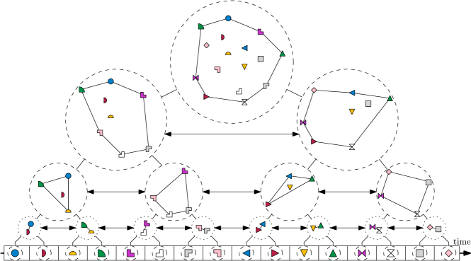
We build a balanced binary search tree $T$ over time with a unique leaf for each temporal point (see Fig. 9). To each node $v\in T$ we associate a canonical subset $C_{v}$. If $v$ is a leaf, then $C_{v}=\{e_{t}\}$ where $e_{t}$ is the temporal point corresponding to $v$, otherwise $C_{v}$ is the union of its children’s canonical subsets. We say that a node $v\in T$ covers the temporal-point $e$ if $e\in C_{v}$.

We will assume that $T$ has been augmented with level-links, pointers between consecutive nodes at the same depth, and an array $A$ of the leaves providing a mapping between temporal points and leaves. So, given any time window $[p_{i},p_{j}]$, we can find a set of $O(\log w)$ canonical sets which cover $[p_{i},p_{j}]$ in $O(\log w)$ time by working up in $T$ from the leaves at $A[i]$ and $A[j]$. Furthermore, at each node $v$, we store the convex hull of $C_{v}$ in clockwise order beginning with the maximum point lexicographically, and we store the index of the point with the minimal coordinates lexicographically, providing access to the entire, upper, and lower hulls.

It is well known that we can find the convex hull of a set of sorted points in linear time using the Graham scan algorithm [20]. Therefore, we construct the tree bottom up from the leaves. Each leaf contains a single point and no processing is required. For each internal node $v$, we merge the sorted lists from the left and right child into a single list for $C_{v}$ in $O(|C_{v}|)$ time. Then we construct the convex hull of $C_{v}$ also in linear time using Graham scan. Each point is stored in at most $O(\log n)$ nodes, and therefore the total space required for $T$ is $O(n\log n)$. We construct each internal node in time linear in the the number of leaves in its subtree, and thus the total time required to construct $T$ is $O(n\log n)$. We summarize this result in the following lemma.

Lemma 2.1.

We can build a decomposition tree $T$ over $n$ events in $O(n\log n)$ time using $O(n\log n)$ space such that given a time window $[p_{i},p_{j}]$, we can find $O(\log w)$ nodes of $T$ which cover $[p_{i},p_{j}]$ in $O(\log w)$ time.

Given a window $[p_{i},p_{j}]$ we call the $O(\log w)$ sub-hulls covering $[p_{i},p_{j}]$ as canonical sub-hulls, and we call the set of canonical sub-hulls the canonical cover of the window. For all the queries in this section, we assume the canonical decomposition has been precomputed.

2.2 Gift Wrapping

A classic algorithm for computing the convex hull is gift wrapping, also known as Jarvis’s March [23]. This technique starts at a point $p_{i}$ on the convex hull and through a comparison of the polar angles of the other points with respect to $p_{i}$ as the center, selects the point $p_{i+1}$, such that all other points are to the right of $p_{i+1}$. If this search is done linearly, the next point on the hull can be found in $O(n)$ time, and thus the entire hull can be computed in $O(nh)$ time. Given a point $q$ on the complete convex hull of a window, clockwise or counterclockwise Gift Wrapping queries, locating the clockwise or counterclockwise adjacent point on the hull, can be done more quickly using our hull decomposition.

Theorem 2.2.

Time-windowed gift wrapping queries on the convex hull of $[p_{i},p_{j}]$ can be answered in $O(\log^{2}w)$ time.

Corollary 1.

The convex hull of $[p_{i},p_{j}]$ can be computed in $O(h\log^{2}w)$.

This technique can be used to answer tangent queries as well, where a tangent query reports the two tangents of the hull passing through a query point $q$ or an exception if $q$ is in the hull.

Corollary 2.

Tangent queries on the convex hull of $[p_{i},p_{j}]$ can be answered in $O(\log^{2}w)$ time.

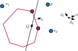
We answer a tangent query via an iterative search; we perform a binary search for the tangent in each sub-hull. Thus, at first it seems that our query time can easily be sped up by a logarithmic factor via standard fractional cascading techniques. However, the answer to a tangent query in one sub-hull may not give us enough information about the answer to a tangent query in another sub-hull. Recall that a convex hull partitions the plane into the region inside the hull, and a set of wedges outside the hull, where each wedge corresponds to the set of query points which will all return the same convex hull point as the answer to a tangent query (see Fig. 3). Note that by moving the query point, we can maintain the same answer to a tangent query on one sub-hull while dramatically changing the answer to the query on other sub-hulls. Thus, there is no clear strategy on how to preprocess the hulls in order to leverage fractional cascading and speed up iterative tangent queries for arbitrary query points.

Figure 1: Gift wrapping.

Figure 2: Tangent query example.

Figure 3: Fractional cascading.

2.3 Linear Programming

In a Linear Programming query, we are given a direction and would like to find a point on the complete convex hull furthest in the queried direction.

Theorem 2.3.

Time-windowed linear programming queries on the convex hull of $[p_{i},p_{j}]$ can be answered in $O(\log w)$ time.

Additionally, we can answer the Line Decision problem, determining if a line intersects the hull.

Corollary 3.

Line decision queries on the convex hull of $[p_{i},p_{j}]$ can be answered in $O(\log w)$ time.

2.4 Line Stabbing

For the Line Stabbing query, a query line, $Q$, is given and we seek the edges of the completed convex hull, if any, that intersect the line. Without loss of generality we will consider the problem of directed line stabbing, i.e., we impose a direction on the query line and return the intersected edge furthest in that direction. We observe that computing convex hull of all pairs of canonical sub-hulls is too inefficient; since they are not separated in space, they may require a linear number of bridge facets.

Figure 4: The point $p$ is extremal for $w$ which is between $u$ and $v$.

Figure 5: The solid region of the complete hull contains the points between the two vector.

Figure 6: The facet normal $n$ is queried and found to improve the right side bound.

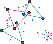
First, we need to define some additional terminology. In Figure 6, we have a few convex hulls and their facet normal vectors. The circular list $D$ consists of all of the normals in the sub-hulls sorted in clockwise order. The vector $w$ is between $u$ and $v$ because $w$ falls between them in the sorted order. The point $p$ is between the two vectors $u$ and $v$ on a convex hull because it is extremal for a vector between $u$ and $v$, namely $w$ or $v$ itself (see Fig. 6). Finally, $v$ and $w$ are adjacent vectors in $D$ if they are consecutive in the angular order.

Lemma 2.4.

If $Q$ intersects the complete hull, then in $O(\log^{2}w)$ time we can find adjacent normals $n_{1}$ and $n_{2}$ in $D$ such that the intersected facet is between $n_{1}$ and $n_{2}$.

Proof 2.5.

Let $d_{1}$ and $d_{2}$ be the left and right perpendicular directions of $Q$, respectively. Then set $\pi_{i}$ to be the extremal point on the complete hull in the direction $d_{i}$ for $i=1,2$. Then we iterate through the canonical cover, considering each canonical sub-hull. Within each sub-hull we iterate through its facet normal vectors $n$. If $n$ is between $d_{1}$ and $d_{2}$, we compute, $p$, the extremal point in the direction $n$. If $p$ is to the left of $Q$, then we set $\pi_{1}=p$ and $d_{1}=n$, otherwise we set $\pi_{2}=p$ and $d_{2}=n$ (see Fig. 6). After processing all of the facet normals in all of the canonical sub-hulls $d_{1}$ and $d_{2}$ will be adjacent vectors. Since we have maintained the invariant that the facet crossing $Q$ is between them, $d_{1}$ and $d_{2}$ are the desired normals. The running time of this algorithm is dominated by the $w$ extremal point queries, each taking time $O(\log w)$ time. However we can speed up the number of linear programming queries by using weighted median selection driven prune and search. To start the search for each convex hull compute the two normals closest to the perpendiculars of $Q$. The number of vectors between these two normals will be the weight for each list and the two normals will dictate the left and right ends of the lists. Then by choosing the weighted median of the medians, a single linear programming query can eliminate a quarter of the remaining weight. Calculating the weighted median takes $O(\log w)$ time and querying the median takes $O(\log w)$ time. Because the hull starts with less than or equal to $w$ total weight, it takes $O(\log w)$ queries to find the adjacent vectors. This gives a total runtime of $O(\log^{2}w)$.

Lemma 2.6.

For two edge normals, $u$ and $v$, that are adjacent in $D$, there are at most $3\log w$ points between $u$ and $v$ on the sub-hulls.

Theorem 2.7.

Time-windowed line stabbing queries on the convex hull of $[p_{i},p_{j}]$ can be answered in $O(\log^{2}w)$ time.

Proof 2.8.

To first establish if the line hits the convex hull we will run two extremal point queries in the directions perpendicular to the line, similar to how we solved the line decision problem. Then we use Lemma 2.4 to find adjacent vectors in $D$ surrounding the edge we seek, in $O(\log^{2}w)$ time. Now, Lemma 2.6 implies there are $O(\log w)$ points between these adjacent vectors on the canonical sub-hulls. So we have $O(\log^{2}w)$ pairs to check. Thus the above algorithm answers line stabbing queries in $O(\log^{2}w)$ time.

Vertical Line Stabbing queries are the special case of line stabbing where the query lines are oriented vertically. Membership queries are to given a point, $p$, decide if $p$ is on the edge of the completed convex hull. These can be contrasted with Containment queries which ask whether a point $p$ is contained by the completed convex hull.

Corollary 4.

Vertical line stabbing, membership, and containment queries on the convex hull of $[p_{i},p_{j}]$ can also be answered in $O(\log^{2}w)$ time.

3 Proximity queries

In this final section we will consider windowed queries based on their proximity. This includes approximate nearest neighbor queries and the construction of proximity graphs.

3.1 Preliminaries

The $Z$-order (or Morton order) is a linear ordering of the points in $\mathbf{R}^{2}$ introduced by Morton in 1962 [31]. This ordering can be described in many ways, but for our purposes it is best understood as the depth-first traversal order of points in a quadtree. We will denote this linear ordering by the symbol $\leq_{Z}$. Considering points in their $Z$-order is a dimension reduction technique that is often used for proximity based data structures  [19, 7].

Lemma 3.1.

Let $P$ be set of points stored in a quadtree, and $C$ a specific quadtree cell storing the points $z_{0},\ldots,z_{k}$ in $Z$-order. If $p$ is a point in $P$ with $z_{0}\leq_{Z}p\leq_{Z}z_{k}$, then $p$ is in $C$

3.2 Hierarchical decomposition

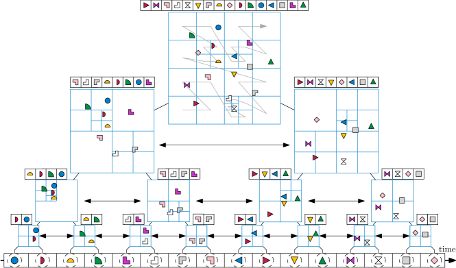
To support proximity queries, we will build a decomposition tree over time, as we did for convex hulls. As before, each node $v$ in the tree corresponds to a canonical subset $C_{v}$, consisting of the points associated with the leaves in its subtree. However, for proximity queries we will be storing the $Z$-order for each of the canonical subsets. This is equivalent to using $2$-dimensional range tree where the first coordinate is a point’s time and the second coordinate is its position in $Z$-order. We will use the standard fractional cascading techniques to speed up queries [12]. In addition to the $Z$-order, we augment each internal node $v$ with a skip-quadtree $Q_{u}$ built over the points in $C_{v}$. For each cell of the quadtree we store the first and last points in the cell according to their $Z$-order. The proof of the following lemma is given in the appendix.

Lemma 3.2.

Any query window of width $w$ can be covered by two canonical subsets $C_{1}$ and $C_{2}$ each of width less than $2w$. Moreover, we can find $C_{1}$ and $C_{2}$ in $O(\log w)$ time.

3.3 Approximate spherical range searching queries

In an approximate spherical range searching query a query point $q$ and radius $r$ are given, and all points whose distance to $q$ is less than or equal to $r$ must be returned and no points whose distance to $q$ is greater than $(1+\epsilon)r$ may be returned, where $\epsilon$ is a fixed constant. The points whose distance to $q$ is between $r$ and $(1+\epsilon)r$ may or may not be reported. Due to space constraints, the proof of the following theorem is given in the appendix.

Theorem 3.3.

Approximate time-windowed $d$-dimensional spherical range reporting queries can be performed in $O(\log w+k)$ time, for any fixed dimension $d\geq 2$.

In our definition of an approximate range query we are assuming regions are perfectly spherical. However, our results can be extended to more general regions using known techniques [16]. Note that in the special case where the query range is an axis aligned rectangle, we can answer an exact orthogonal range query in optimal time using known techniques. In the orthogonal range searching problem we are given a collection points in the plane and an axis aligned query rectangle from which we must report the set of points contained within the rectangle. Alstrup et al. [3] give a solution for orthogonal range searching in $\mathbf{R}^{3}$ using $O(n\log^{1+\epsilon}n)$ space and $O(\log n+k)$ query time. Simply by treating time as a spatial dimension, this allows us to answer windowed $2$-dimensional orthogonal range searching queries.

3.4 Approximate nearest neighbor queries

Given a set of points $P$ and query point $q$ an $\epsilon$-approximate nearest neighbor query asks for a point $p$ in $P$ whose distance to $q$ is at most $(1+\epsilon)r$ where $r$ is the distance to $q$’s nearest neighbor in $P$. The following lemma establishes a relationship between approximate nearest neighbor queries on multidimensional points and successor queries in the $Z$-order of those points. Recall that in the successor query problem we are given a set of points $A$ on the real line and a query point $q$ on the line, and we must report the smallest element in $A$ greater than $q$.

Lemma 3.4 (Liao, Lopez and Leutenegger [27]).

Let $P$ be a set of points in $R^{d}$. Define a constant $c=\sqrt{d}(4d+4)+1$. Suppose that we have $d+1$ shifted lists $P+v^{j}$ for $j=0,\ldots,d$ (the specific values of $v^{j}$ are given in [27]) , each one sorted according to its $Z$-order. We can find a query point $q$’s $c$-approximate nearest neighbor in $P$ by examining the $2(d+1)$ predecessors and successors of $q$ in the lists.

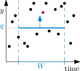
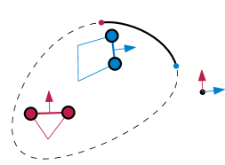
In the windowed model, a successor query corresponds to a two-dimensional geometric query, where the time of a point maps to its $x$ coordinate, and the value of the point maps to its $y$ coordinate. To find the successor of value $q$ in window $[t_{1},t_{2}]$, we slide a horizontal line segment $[(t_{1},q),(t_{2},q)]$ upward, and the first point we hit is the answer (see Fig. 8).

We can answer windowed successor queries in $O(n\log n)$ space and $O(\log w)$ time per query using a structure similar to a $2$-d range tree. We build a decomposition tree over the time of the points, where each internal node stores the points in its canonical set sorted by value. We answer a query by performing a successor query at each of the $O(\log w)$ nodes which together cover the window, and we speed up the iterative queries at the internal nodes using fractional cascading.

Now, we can leverage our windowed successor data structure to answer windowed approximate nearest neighbor queries. In each node of our decomposition tree we store $d+1$ copies of its canonical set, sorted according to the $d+1$ shifted versions of the $Z$-order from Lemma 3.4. Given a query point $q$ and window $W=[p_{i},p_{j}]$, we find the windowed successor and predecessor in each of the shifted $Z$-orders. By Lemma 3.4, one of the $2(d+1)$ points which is closest points is guaranteed to be a $c$-approximate nearest neighbor of $q$.

Now, we refine our answer to an $\epsilon$-nearest neighbor via a binary search over potential distances to the $\epsilon$-nearest neighbor. The refinement process requires $O(\log\frac{1}{\epsilon})=O(1)$ approximate spherical emptiness queries [4]. For this strategy to work in the windowed model, we must support windowed approximate spherical emptiness queries, which can be done with minor modifications to our windowed approximate range query structure. Namely, we report only the first point found, or empty if the range is empty. This means the entire binary search takes $O(\log w)$ time to complete. Thus, we have proven the following theorem.

Theorem 3.5.

Approximate time-windowed nearest neighbor queries in $\mathbf{R}^{d}$ can be performed in $O(\log w)$ time, for fixed $d\geq 2$.

3.5 Proximity graph constructions

Finally, we can use these methods to construct most interesting proximity graphs in linear time. As first step we use our $Z$-order decomposition tree to find a set of canonical subsets exactly covering our query window, taking $O(\log w)$ time. Then we merge their $Z$-orders into a $Z$-order for the points in the query window, taking $O(w)$ time. From the $Z$-order we compute the compressed quadtree from of the points in $O(w)$ time [10], and from the compressed quadtree we compute the well-separated pair decomposition also in linear $O(w)$ time [29]. With the well-separated pair decomposition the following can be constructed in $O(w)$ time: Delaunay triangulation, minimum spanning tree, nearest neighbor graph and Gabriel graph [29].

Appendix A Skyline

Figure 7: Stabbing inequality

In this section, we form a general method for answering queries for the set of maximal elements under a preordered relation and then specialize this method to the problem of computing the skyline . Previously the problem of computing the skyline for a fixed-width sliding window was considered by Lin et al. [28]. The fastest algorithms for skyline run in time $O(n\log^{d-3}n)$ in the worst case for points in $\mathbf{R}^{d}$ for fixed $d\geq 4$ [11], and the fastest output sensitive algorithms run in time $O(n\log^{d-2}k)$ for fixed $d\geq 3$ [24].

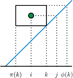
Given a set, $S,$ a binary relation, $<$, is said to be an (irreflexive) preorder if (1) for all $a\in S$, $a\not<a$ (irreflexive); (2) for all $a,b,c\in S$ if $a<b$ and $b<c$, then $a<c$ (transitive). An element, $x$, in a subset, $E$, of $S$ is said to be maximal in $E$ if there does not exist a $y\in E$ with $x<y$. Finally, given a sequence, $e_{i}$ for $0\leq i<n$, of elements from a preordered set $S$ we define for each element $e_{k}$ the function $\phi(k)$ to be the largest $j^{\prime}$ such that $e_{k}\not<e_{j}$ whenever $k\leq j\leq j^{\prime}$; and, $\pi(k)$ to be the smallest $i^{\prime}$ such that $e_{k}\not<e_{i}$ whenever $i^{\prime}\leq i\leq k$. An element $e_{k}$ is a maximal element of $[e_{i},e_{j}]$ precisely when $pi(k)\leq i$ and $j\leq\phi(k)$, yielding the following lemma illustrated in Fig. 7.

Lemma A.1.

An element $e_{k}$ is a maximal element of the set $[e_{i},e_{j}]$ if and only if $\pi(k)\leq i\leq k\leq j\leq\phi(k)$; equivalently, $e_{k}$ is a maximal element of the set $[e_{i},e_{j}]$ if and only if the point $(i,j)$ stabs the rectangle $[\pi(k),k]\times[k,\phi(k)]$.

In general, the method for computing $\phi$ is to initialize a data structure $C$. Then process the temporal-points in order. For each temporal-point $e_{k}$ we query $C$ to find and set $\phi[e]=k$ for all elements $e$ less than $e_{k}$. Then these points are removed from $C$ and $e_{k}$ is added to $C$. The computation of $\pi$ uses the same algorithm, but processes points in reverse order. With $\phi$ and $\pi$ computed, the problem is now reduced to the rectangle stabbing problem, for which we use existing data structures.

Lemma A.2 (Eppstein et al. [17] and Agarwal et al. [1]).

A set of $n$ rectangles whose endpoints lie on the grid $[0,n]\times[0,n]$ can be preprocessed into a data structure of size $O(n^{1+\epsilon})$ in $O(n^{1+\epsilon})$ time that can report the rectangles stabbed by a query point in $O(k)$ time and count them in $O(1)$ time, where $k$ is the number of rectangles reported. If the rectangles are colored, the set of distinct colors stabbed can be reported in time $O(k)$, where $k$ is the number of colors reported.

Lemma A.3.

A sequence of elements, $e_{i}$ for $0\leq i<n$, from a preordered set can be preprocessed into a data structure of size $O(n^{1+\epsilon})$ in time $O(n^{1+\epsilon})$ that can report the maximal elements in a window $[e_{i},e_{j}]$ in $O(k)$ time where $k$ is the number of reported elements, assuming that $\pi$ and $\phi$ can be computed in $O(n^{1+\epsilon})$ time.

The skyline of a set of points in $\mathbf{R}^{d}$ is defined to be the maximal elements in the set under the dominance relation where a point $p$ is said to be dominated by a point $p^{\prime}$ if $p[i]\leq p^{\prime}[i]$ for $0\leq i<d$ and $p\neq p^{\prime}$. So our general method applies, for computing the skyline. Mortensen presents a dynamic data structure for dominance queries in $\mathbf{R}^{d}$ that supports insertion and deletion of points in $O(\log^{d}n)$ time and reporting of all points dominated by a given query point in $O(\log^{d}n+k)$ time where $k$ is the number of reported points [30]. We can use this data structure to compute $\phi$ and $\pi$ for the dominance relation in $O(n\log^{d}n)$. So by Lemma A.3 we have following theorem.

Theorem A.4.

A sequence of temporal points, $p_{i}$ for $0\leq i<n$, in $\mathbf{R}^{d}$ can be preprocessed into a data structure of size $O(n^{1+\epsilon})$ in $O(n^{1+\epsilon})$ time such that a query for the skyline of $[p_{i},p_{j}]$ can be reported in $O(k)$ time. Furthermore, if the points are colored then the distinct colors on the skyline can be reported in $O(k)$ time.

Appendix B Omissions from Section 2

Proof B.1 (Theorem 2.2).

We first compute the canonical cover. Then for each of the canonical sub-hulls we perform a binary search over its points, locating the point $p$ such that the vector from $q$ to $p$ forms the maximal angle with the positive $x$-axis. Then, from these $O(\log w)$ points, we choose the point with maximal angle, completing our gift wrapping query (see Fig. 3). The total time is dominated by the $O(\log^{2}w)$ time for the binary searches. A counterclockwise gift wrapping query is answered in a similar manner.

Proof B.2 (Corollary 1).

To compute the full convex hull of $[p_{i},p_{j}]$, we begin by locating a point we know to be on the hull, e.g., the point with the lowest $x$-value, which can be done in $O(\log w)$. We then perform gift wrapping queries in $O(\log^{2}w)$ time per query until the whole hull is returned. Since we perform one query per point on the hull, we perform $h$ before returning to our starting point. Therefore we can compute the entirety of the hull in $O(h\log^{2}w)$ time.

Proof B.3 (Corollary 2).

We first perform a containment query (Corollary 4) in $O(\log^{2}w)$ time, returning an exception if the query point is contained in the hull. Now, given a point $q$ outside the convex hull we suppose that $q$ is on the hull, and performing a gift wrapping in clockwise and counterclockwise directions in $O(\log^{2}w)$ time. Producing the requested tangents.

Proof B.4 (Theorem 2.3).

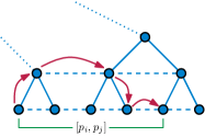
For this query it suffices to solve the problem for each of the canonical sub-hulls, and then return the solution that is furthest in the query direction. Since this is an iterative searching problem, we can use fractional cascading [12]. For our decomposition tree our catalog graph is of $O(1)$ degree, as each decomposition node connects to at most one ancestor, two children, and a left and right node via level-links (see Fig. 9). This allows us to construct a recursive relation between augmented catalogs, in which we share every sixteenth element and create sufficient bridge pointers to allow constant time subsequent searches, while still maintaining storage and preprocessing proportional to the size of the decomposition node. This cascading structure allows us to solve the query in $O(\log w)$ time. This query does not take $O(\log n)$ time because, beginning at the edge of our window, we can navigate through our fractional cascading structure without routing outside of the window space (see Fig. 3).

Proof B.5 (Corollary 3).

This query reduces to two extremal point queries in the directions perpendicular to the line. The two extremal points are separated by the query line if and only if the line intersects the convex hull.

Proof B.6 (Lemma 2.6).

Suppose there are four or more points in a sub-hull between the two edge normals. Then there are at least three edges in that sub-hull with normals between $u$ and $v$ one of which must be strictly between $u$ and $v$. However $u$ and $v$ were adjacent in the complete list of edge normals. This is a contradiction so there must be less than four points between $u$ and $v$ in each sub-hull. Because there are at most $\log w$ sub-hulls, the total number of points between $u$ and $v$ is $3\log w$.

Proof B.7 (Corollar 4).

Vertical line stabbing queries are solved by the above algorithm. Membership and containment queries can both be answered with line stabbing queries of lines passing through the query points. If the two edges found surround $p$ then we know it is contained in the convex hull and if $p$ is on either edge then we know it is a member of the hull.

Appendix C Omissions from Section 3

Proof C.1 (Lemma 3.2).

Let $W=[p_{i},p_{j}]$ be a window of width $w$. Set $C_{1}$ to be the largest canonical subset containing $p_{i}$ of width less than $2w$, and set $C_{2}$ to be the canonical subset adjacent to $C_{1}$ in level link list in the direction of increasing time. These sets can be found by following parent pointers for at most $O(\log w)$ levels. Finally since the widths of $C_{1}$ and $C_{2}$ are at least $w$ they cover $W$.

Proof C.2 (Theorem 3.3).

Let $W=[p_{i},p_{j}]$ be a window of width $w$. To perform a query with $W$ we first use Lemma 3.2 to find two canonical subsets $C_{u}$ and $C_{v}$ covering our query window, corresponding to nodes $u$ and $v$ in the decomposition tree, in $O(\log w)$ time. Then we search the quadtrees $Q_{u}$ and $Q_{v}$ to find their respective sets of inner cells (cells entirely contained in the approximate region) $\mathcal{I}_{u}$ and $\mathcal{I}_{v}$ each set of size $O(\epsilon^{1-d})$ where $d$ is the dimension. This can be done in $O(\log w+\epsilon^{1-d})=O(\log w)$ time [16].

Then for each of the inner cells $I\in\mathcal{I}_{u}\cup\mathcal{I}_{v}$ we perform a $2$-dimensional range reporting query with the rectangle $[p_{i},p_{j}]\times[z_{0},z_{1}]$, where $z_{0}$ and $z_{1}$ are the first and last point in $I$ in $Z$-order, and record the union of the points reported in $O(\log w+k)$ time where $k$ is output size. By a simple packing argument, the total number of inner cells is bounded by a function of the constants $\epsilon$ and $d$ [19]. Thus, the total time for the query is $O(\log w+k)$.

By construction we have that $W\subseteq C_{u}\cup C_{v}$, i.e. all points in the window $W$ are contained in leaves of either $T_{u}$ or $T_{v}$. Furthermore, the set of inner cells produced contain all geometric points in the approximate query range independent of their time stamp. The query rectangle at each inner cell guarantees that we return precisely the set of points contained in that cell which also have timestamps in the query window. Thus, returned points are exactly the set of points which are both temporally in the window $W$ and geometrically in the approximate range.

Appendix D Omitted Figures

Some figures which are not legible in the two column format are included on the following page.

Figure 8: Windowed successor query.

Figure 9: Decomposition tree of temporal points. Each temporal point has a corresponding geometric point with coordinates in $\mathbf{R}^{2}$. Each node stores the convex hull of the points in its subtree.

Figure 10: Decomposition tree over temporal points. Each temporal point has a corresponding geometric point with coordinates in $\mathbf{R}^{2}$. Each node stores the quadtree and z-order of the points in its subtree.

References

- [1] Agarwal, P.K., Govindarajan, S., Muthukrishnan, S.: Range Searching in Categorical Data: Colored Range Searching on Grid. In: ESA, LNCS, vol. 2461, pp. 17–28. Springer (2002)
- [2] Agarwal, P.K., Sharir, M.: Off-line dynamic maintenance of the width of a planar point set. Computational Geometry 1(2), 65–78 (1991)
- [3] Alstrup, S., Brodal, G.S., Rauhe, T.: New data structures for orthogonal range searching. In: FOCS. pp. 198–207 (2000)
- [4] Arya, S., Da Fonseca, G.D., Mount, D.M.: A unified approach to approximate proximity searching. In: ESA. pp. 374–385. Springer (2010)
- [5] Bannister, M.J., DuBois, C., Eppstein, D., Smyth, P.: Windows into relational events: Data structures for contiguous subsequences of edges. In: SODA. pp. 856–864 (2013)
- [6] Basch, J., Guibas, L.J., Hershberger, J.: Data Structures for Mobile Data. In: SODA. pp. 747–756 (1997)
- [7] Bern, M., Eppstein, D., Teng, S.H.: Parallel construction of quadtrees and quality triangulations. Int. J. Comp. Geom. & App. 09(06), 517–532 (1999)
- [8] Börzsönyi, S., Kossmann, D., Stocker, K.: The Skyline Operator. In: ICDE. pp. 421–430 (2001)
- [9] Chan, T.M.: Dynamic planar convex hull operations in near-logarithmaic amortized time. J. ACM 48(1), 1–12 (2001)
- [10] Chan, T.M.: Well-separated pair decomposition in linear time? Inf. Process. Lett. 107(5), 138 – 141 (2008)
- [11] Chan, T.M., Larsen, K.G., Patrascu, M.: Orthogonal range searching on the RAM, revisited. In: Symp. on Comp. Geom. pp. 1–10 (2011)
- [12] Chazelle, B., Guibas, L.J.: Fractional cascading: I. A data structuring technique; II. Applications. Algorithmica 1(1-4), 133–191 (1986)
- [13] Driscoll, J.R., Sarnak, N., Sleator, D.D., Tarjan, R.E.: Making data structures persistent. J. of Comp. and System Sci. 38(1), 86–124 (1989)
- [14] Edelsbrunner, H., Overmars, M.H.: Batched dynamic solutions to decomposable searching problems. J. Algorithms 6(4), 515–542 (1985)
- [15] Ehrgott, M., Gandibleux, X.: Multiple Criteria Optimization: State of the Art Annotated Bibliographic Surveys. Kluwer Academic Publishers (2002)
- [16] Eppstein, D., Goodrich, M.T., Sun, J.Z.: The skip quadtree: a simple dynamic data structure for multidimensional data. In: Symp. on Comp. Geom. pp. 296–305. SCG ’05, ACM (2005)
- [17] Eppstein, D., Muthukrishnan, S.: Internet packet filter management and rectangle geometry. In: SODA. pp. 827–835 (2001)
- [18] Erwig, M., Güting, R.H., Schneider, M., Vazirgiannis, M.: Abstract and discrete modeling of spatio-temporal data types. In: 6th ACM GIS. pp. 131–136 (1998)
- [19] Goodrich, M.T., Simons, J.A.: Fully Retroactive Approximate Range and Nearest Neighbor Searching. In: Algorithms and Computation, LNCS, vol. 7074, pp. 292–301. Springer (2011)
- [20] Graham, R.L.: An Efficient Algorithm for Determining the Convex Hull of a Finite Planar Set. Inf. Process. Lett. 1(4), 132–133 (1972)
- [21] Grossi, R., Italiano, G.F.: Efficient Splitting and Merging Algorithms for Order Decomposable Problems. Information and Computation 154(1), 1–33 (1999)
- [22] Hershberger, J., Suri, S.: Off-Line maintenance of planar configurations. J. Algorithms 21, 453–475 (1996)
- [23] Jarvis, R.A.: On the identification of the convex hull of a finite set of points in the plane. Inf. Process. Lett. 2, 18–21 (1973)
- [24] Kirkpatrick, D.G., Seidel, R.: Output-size sensitive algorithms for finding maximal vectors. In: Symp. on Comp. Geom. pp. 89–96 (1985)
- [25] van Kreveld, M.J., Overmars, M.H.: Concatenable Structures for Decomposable Problems. Information and Computation 110(1), 130–148 (1994)
- [26] Kung, H.T., Luccio, F., Preparata, F.P.: On Finding the Maxima of a Set of Vectors. J. ACM 22(4), 469–476 (October 1975)
- [27] Liao, S., Lopez, M., Leutenegger, S.: High dimensional similarity search with space filling curves. In: 17th Int. Conf. on Data Engineering. pp. 615–622 (2001)
- [28] Lin, X., Yuan, Y., Wang, W., Lu, H.: Stabbing the Sky: Efficient Skyline Computation over Sliding Windows. In: ICDE. pp. 502–513 (2005)
- [29] Löffler, M., Mulzer, W.: Triangulating the Square and Squaring the Triangle: Quadtrees and Delaunay Triangulations are Equivalent. SIAM J. Comput. 41(4), 941–974 (2012)
- [30] Mortensen, C.W.: Fully Dynamic Orthogonal Range Reporting on RAM. SIAM J. Comput. 35(6), 1494–1525 (2006)
- [31] Morton, G.M.: A computer Oriented Geodetic Data Base; and a New Technique in File Sequencing. Technical Report, IBM Ltd. (1966)
- [32] Roddick, J.F., Spiliopoulou, M.: A bibliography of temporal, spatial and spatio-temporal data mining research. SIGKDD Explor. Newsl. 1(1), 34–38 (1999)
- [33] Shi, Q., JaJa, J.: Techniques for indexing and querying temporal observations for a collection of objects. In: ISAAC. LNCS, vol. 3341, pp. 822–834. Springer (2004)