Drawing Graphs within Restricted Area

Abstract

We study the problem of selecting a maximum-weight subgraph of a given graph such that the subgraph can be drawn within a prescribed drawing area subject to given non-uniform vertex sizes. We develop and analyze heuristics both for the general (undirected) case and for the use case of (directed) calculation graphs which are used to analyze the typical mistakes that high school students make when transforming mathematical expressions in the process of calculating, for example, sums of fractions.

1 Introduction

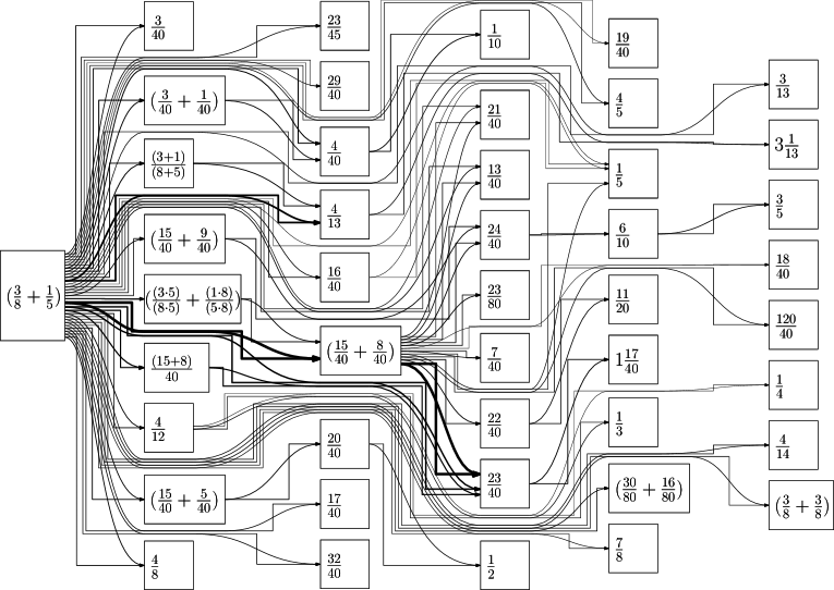
Our motivation for the problem that we study in this paper stems from so-called calculation graphs. Calculation graphs represent calculations starting from some initial task. They are used in studies [11] involving large numbers of high school students in order to analyze the students’ typical mistakes in elementary mathematics. Even for relatively simple tasks such as evaluating the term “$3\cdot(2+1/5)$”, the different transformations performed by a large number of subjects can result in calculation graphs with hundreds of vertices. With the help of drawings of calculation graphs, human experts should be able to analyze how students calculate and, especially, which mistakes they frequently make. As Hennecke [11] suggests, such drawings are only useful if they are not too large, that is, if they fit into a relatively small drawing area. Hence, well-readable drawings of important parts of the graphs must be generated in an automated fashion. Certainly, the drawn subgraph should represent as much information of the original calculation graph as possible. Therefore, we consider the graphs to be edge- and vertex-weighted; see Fig. 1 for an example.

Figure 1: Example of a calculation graph. Edge weights are indicated on the edges.

The weight of an edge is the number of students who applied the respective calculation step; the weight of a vertex is the number of students who had the given term as an intermediate result in their calculation. Since we want the labels of the vertices to be readable, we assume that their sizes are fixed. Hence, often only a small fraction of the graph will fit into the prescribed drawing area. Note that a user of such a drawing must be made aware that only a subgraph is shown.

Certainly, vertices and edges that occur only in a single student’s calculation can easily be dropped. For higher weights, however, this is not as easy. For instance, it could be possible that dropping a single vertex of medium weight allows us to include several other vertices in the drawing, each having almost the weight of the dropped vertex; the resulting drawing can therefore allow a better analysis. Hence, we develop a method for selecting the drawn subgraph based on the graph structure and not only on the weights.

Further Examples.

Apart from calculation graphs, there are also other scenarios in which most of the information of a large graph should be presented in a limited area to the user. A first example are social networks, which are usually very large. In this setting, both labels of the vertices and weight (e.g., given by the person’s activity in the network) occur. By drawing a heavy subgraph in a restricted area, a user can quickly get an overview over important actors in the network and the connections between them. Another example, that we will use in the main part of the paper, are coauthor networks, where the weights represent numbers of publications. Here, we want to find a drawing of a subgraph that represents as many of the publications as possible, i.e., we prefer to keep authors with many publications.

Related Work.

Surprisingly, the very natural problem of selecting a subgraph that can be drawn within a prescribed area seems to be new. Some work on related problems, however, is worth being mentioned. Rather than fixing the drawing area and maximizing the size of the subgraph that fits into this area, graph drawing research has focussed on drawing the whole input graph and minimizing the area needed for the drawing, which has also been the task in graph drawing contests [4]. This problem is known to be NP-hard for orthogonal drawings with given orthogonal representation (that is, fixed bends) [12]. In constrained graph layout [10, 7], the user can constrain the region into which a vertex must be placed. Dwyer et al. [6] presented the algorithm IPSep-CoLa that allows constraints demanding a vertical or horizontal separation of vertex labels. Especially, the constraints allowed in their algorithm make it possible to enforce that vertices are placed within a prescribed area. However, in contrast to our work, they do not consider dropping vertices. If the vertices do not fit into the area, their algorithm will not find a feasible drawing. The well-known algorithm of Fruchterman and Reingold [8] for force-directed graph drawing allows to specify a rectangular area within which the whole graph has to be drawn. However, in contrast to our work, the algorithm can easily achieve this since vertices are drawn as points without label and edges can be made arbitrarily short, which we do not allow.

Dwyer et al. [5] developed a method for interactive exploration of graphs based on constrained graph layout. In their method, they use a fast heuristic for the overview drawing; for the detailed view of a smaller part of the graph, however, they can afford to use a slower constrained graph layout algorithm that yields better results. Constraints are used in order to ensure consistency between the views and preserve the users’s mental map. Da Lozzo et al. [3] considered the problem of drawing graphs on the very small display of a smartphone. In contrast to the approach used in this paper, the did not try to represent the whole graph on the display, but rather decided to provide only a local view around a focus vertex; their approach then offers interactive ways of navigating through the graph and exploring the graph based on the local view.

Our contribution.

While calculation graphs have quite specific characteristics and drawing requirements (see Section 3), the problem of graph drawing under area restrictions is also of interest for general, undirected graphs. For both cases, we present heuristics and evaluate them experimentally.

For the general case, we use the force-directed approach, reusing forces defined by Fruchterman and Reingold [8] and by Bertault [1]. We add extra phases in which the graph is pressed together; from time to time we remove vertices or edges from the graph if this is needed for further compaction. We use the desired edge length as parameter both for the usual iterations and our extra phases. In our tests, this proved to be effective for parametrizing the density of the output drawing. Furthermore, we experimentally improved the way of avoiding vertex-edge intersections and we developed a postprocessing that routes some of the edges as curves.

For calculation graphs, we chose the well-known Sugiyama framework [15] as basis for our algorithm since we want calculation paths to be readable from left to right. We add a method that successively removes the least important vertices and edges until the drawing fits into the given area. We also consider the weight of edges for crossing minimization so that important edges have few crossings. In our tests, it turned out that removing the lightest vertices as a preprocessing often improved the weight of the final subgraph. Furthermore, routing the edges as curves gave very nice results, also compared to the original orthogonal drawing style for calculation graphs.

2 General Graphs

We first present an algorithm for drawing arbitrary graphs. The input of our problem consists of an unweighted graph $G=(V,E)$ with a weight function $w\colon V\cup E\to\mathbb{R}^{+}$. For each vertex $v\in V$, we are given a geometric object $\ell(v)$ that will represent the vertex in the drawing. Vertices can be represented by different shapes, e.g., rectangles, disks, or ellipses. We will focus on rectangular vertices which are well-suited for text labels of vertices. We will denote the height and the width of $\ell(v)$ by $h_{v}$ and $w_{v}$, respectively.

In addition to the graph input, we are given an axis-parallel rectangle of height $H$ and width $W$, the drawing area. The task is to find a subgraph $G^{\prime}=(V^{\prime},E^{\prime})$ of $G$ with a nice drawing of $G^{\prime}$ within the given drawing area.

The hard constraints for the drawing are clear: Each vertex $v\in V^{\prime}$ must be represented by $\ell(v)$, the vertices must not overlap, and each edge must connect its incident vertices. However, it needs to be clarified, what a nice drawing is. In our setting with a restricted drawing area, putting vertices close together can allow us to have more vertices—and thus more weight—in the final drawing. Certainly, a drawing with vertices that are very close is not nice; the same holds for very short edges. We will discuss these criteria and more later in detail.

By a straightforward reduction from Subset Sum, where we use height 1 for all vertices and the drawing area, we can easily observe that maximizing the weight of the subgraph that can be drawn in a prescribed area is NP-hard.

2.1 Our Algorithm

Our approach makes heavy use of the force-directed framework; in this class of graph drawing algorithms, the drawing is incrementally improved, starting with an arbitrary layout. Each improvement step is done by letting forces, defined using physical analogies, move the vertices.

In contrast to usual force-directed algorithms, we have to take both the dimensions of vertices and of the prescribed drawing area into account. Therefore, we add two important ingredients: We try to fit the drawing into a frame of decreasing size, and we remove vertices or edges from the graph in order to make the graph smaller so that the current drawing can fit into the current frame. While, as a first idea, fitting the drawing into the given area could be steered by a force pulling all vertices towards the center of the drawing region, this idea has some drawbacks. Therefore, we will introduce a more advanced approach. Similarly, removing vertices could simply be done by removing the lightest vertex in each step. However, this would take neither the structure of the graph nor the current drawing into account. Hence, we introduce a measure for the stress of vertices in the current situation; we will always remove the vertex with the highest stress value. Algorithm 1 in Appendix 0.A.1 outlines the basic structure of our algorithm. In the following paragraphs, we will detail out the individual steps.

Forces.

We first define the forces used in our algorithm.

• We reuse existing forces from the algorithm of Fruchterman and Reingold [8]; that is, for any pair $u,v\in V$ of vertices, there is a force $F_{\mathrm{r}}\left(u,v\right)=l_{\mathrm{unit}}^{2}/(d\left(u,v\right))\cdot\overrightarrow{uv}$ on $v$ that repels $v$ from $u$, where $\overrightarrow{uv}$ is the unit vector pointing from $u$ towards $v$. If the vertices are adjacent, that is, if $uv\in E$, there is an additional force $F_{\mathrm{a}}(u,v)=(d(u,v))^{2}/l_{\mathrm{unit}}\cdot\overrightarrow{vu}$ that attracts $v$ towards $u$. Both forces use a factor $l_{\mathrm{unit}}$ which describes the desired unit edge length. Since the desired edge length heavily influences the density of the drawing, and, hence, the number and weight of vertices and edges that can be placed within the given drawing area, the choice of $l_{\mathrm{unit}}$ is crucial for the results. While we allow the parameter to be set freely, we stress that the value must be chosen carefully, taking the sizes of vertices into account, so that one gets nice output drawings.

• Due to the high density of the input graphs and the given sizes of vertices, it may easily occur that vertices are intersected by nonincident edges, which reduces the readability significantly. As a first step to overcome this problem, we use a force that has been introduced by Bertault in his PrEd algorithm [1]: If an edge $\left\{u,w\right\}$ intersects a vertex $v$ in its inner region, that is, close to the center of $v$, then we let a force $F_{\mathrm{e}}\left(v,\left\{u,w\right\}\right)={\left(l_{\mathrm{unit}}-d\left(v,i_{v}\right)\right)}^{2}\cdot\overrightarrow{i_{v}v}$ repel $v$ from $\left\{u,w\right\}$, where the point $i_{v}$ is the orthogonal projection of $v$ onto the straight-line segment $\overline{uw}$. Note that this does not guarantee that intersections between vertices and edges are avoided. However, such intersections become less likely; in Sec. 2.2, we will see how their number can be further reduced by routing edges as curves.

• For making the drawing more compact, we introduce a force $F_{\mathrm{g}}(v)=d\left(v,p_{\mathrm{c}}\right)\cdot\overrightarrow{vp_{\mathrm{c}}}$ that attracts each vertex $v$ to the center $p_{\mathrm{c}}$ of the drawing area. In our experiments it turned out that activating this force in later steps of the algorithm reduces the time for finding a final drawing, but also the quality of the output. Therefore, as a default, the force is only active when computing the very first equilibrium layout.

Handling the Frame.

The forces described above yield a functional force-directed algorithm which can be applied for getting an initial layout. Once we have an initial drawing, we initialize the frame $F$ as the bounding box of the drawing. Our algorithm iteratively reduces the size of the frame until it matches the prescribed drawing area.

In each step, we first uniformly reduce the height and the width of $F$ by a small amount. It may happen that some vertices (partially) lie outside of the resulting new frame $F^{\prime}$. If this is the case for a vertex $v$, we just place it at the closest position that lies completely within $F^{\prime}$. This operation can result in intersections of vertices. Therefore, we compute a new equilibrium state which hopefully solves the intersections.

In all force-directed iterations in which there is a frame, we will always ensure that no vertex leaves the frame. This is done by cutting off the resulting movement vectors; Fruchterman and Reingold [8] did the same for ensuring that no vertex leaves the drawing area in their algorithm—with the difference that they did not shrink the frame but rather started with a very compressed drawing since in their setting vertices are points that can be arbitrarily close.

If there are intersections after computing a new equilibrium layout, we have a clear indication that the graph is still too large for the current frame and, hence, for the desired drawing area. In this case, and also in some more cases, we will remove vertices or edges as described in the next section.

Removing Vertices and Edges.

Our indicator for the necessity of the removal of vertices or edges is, roughly speaking, the density of the drawing. If there are too many vertices in the graph for the current frame, then vertices will come very close. Therefore, we decide to remove a vertex or an edge if the minimum edge length is less than a value $l_{\mathrm{adj}}$ or if the minimum distance between two nonadjacent vertices is less than a value $l_{\mathrm{nadj}}$. Note that this includes the case of two intersecting vertices.

Deciding what should be removed is more difficult. Since we want to keep as much weight as possible, the natural idea is to remove the lightest vertex. However, this is often not the best choice—even if it is unambiguous. A more advanced criterion should take also the degree of a vertex into account. The higher the number of neighbors of a vertex is, the more information on the graph is lost by removing the vertex.

Stress Calculation.

However, we can still do better: So far, we have not taken the current drawing into account, although it can give us valuable information about the density of vertices in the vicinity of the vertex that should be removed. Thus, we suggest doing so by considering the forces in the last equilibrium layout. Even if the total movement vector of a vertex has length zero, this may actually result from strong forces that try to move the vertex to different directions, e.g., if the vertex is “trapped” between many other vertices around it.

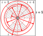
These considerations lead us to a measure that we call the pressure of a vertex. Intuitively, the pressure is the maximum strength of forces in roughly opposite directions that act on a vertex. For formalizing this, we subdivide all force vectors applied on the vertex $v$ into eight octants. For each octant, we sum up the force vector. For $i=0,\ldots,7$ let $l_{i}$ be the length of the resulting force vector for octant $i$. Now, we first build the pressure $p_{i}$ for octant $i$ by comparing $l_{i}$ with the force vectors in the three opposite directions, i.e., with $l_{i+3}$, $l_{i+4}$, and $l_{i+5}$ ($\mathrm{mod}~{}8$); see Fig. 2. The pressure then is the maximum over the pairwise minima, i.e., $p_{i}=\max\left\{\min\left\{p_{i},p_{i+3}\right\},\min\left\{p_{i},p_{i+4}\right\},\min\left\{p_{i},p_{i+5}\right\}\right\}$. The total pressure on $v$ is $p(v)=\max\left\{p_{0},\ldots,p_{7}\right\}$.

Figure 2: Pressure computation for one of the octants.

Now, we must integrate the weight $w(v)$ and the degree $\deg(v)$—indicators of the vertex’s resistance against pressure—with the pressure in order to get the stress $s(v)$. We do so by setting $s(v)=p(v)/(w(v)\cdot(\deg(v)+c_{\deg}))$. Here, $c_{\deg}$ is a small positive constant that ensures that we do not get problems for isolated vertices and that steers our preference for keeping isolated vertices in the drawing. With this definition of the stress, we can always choose the vertex with the highest stress for removal.

Boundary Vertices.

There is a special case for vertices close to the boundary of the frame. We never move a vertex over the boundary although, in many cases, vertices are repelled in this direction by the inner vertices. This phenomenon is a cause of pressure on a vertex that is, so far, not covered by our definition. We therefore introduce a new “virtual” force that mimics the resistance against movements that push the vertex out of the frame. This force repels the vertex perpendicularly to the inside of the frame, away from the closest point $p_{\mathrm{f}}$ of the frame’s boundary. More precisely, the virtual force is $F_{\mathrm{f}}(v)=\overrightarrow{p_{\mathrm{f}}v}\cdot l_{\mathrm{unit}}^{2}/d(v,p_{\mathrm{f}})$. We stress that $F_{\mathrm{f}}$ is only taken into account for the stress computation and not actually applied.

Edges.

In some cases, one may try to remove only an edge instead of a whole vertex; the hope is that after removing the edge, the graph becomes more flexible so that the available space can be used better. As an indicator for such a situation, we use the average edge length in the current drawing. If this length is larger than $l_{\mathrm{unit}}\cdot c_{\mathrm{len}}$, with a factor $c_{\mathrm{len}}>0$, we decide for removing an edge instead of a vertex. The intuition is that, on average, the edges are not very short, which means that by removing one of these longer edges we could allow more flexibility to the placement of vertices.

In order to determine which edge will be removed, we, again, use a definition of stress. To this end, we take both the weight $w(e)$ and the weights of the edges crossing $e$ into account. Let $E^{\prime}$ be the set of these edges. Then, we set $s(e)=\sum_{e^{\prime}\in E^{\prime}}w(e^{\prime})\cdot|E^{\prime}|/w(e)$ to be the stress of $e$, and we remove the edge with the highest stress value.

2.2 Extensions

We developed and implemented two extensions that can help improve the runtime of the algorithm and the quality of the resulting drawings, respectively.

Preprocessing.

In many input instances, there is a large number of vertices with very small weight, for which it is very unlikely to occur in the final drawing. To speed up the algorithm, we can remove all vertices that are lighter than a threshold value $w^{\star}$. Our choice of $w^{\star}$ is based on guessing a bound on the maximum number of vertices in the final drawing and depends on the height $H$ and the weight $W$ of the drawing area, the minimum height $h_{\min}$ and the minimum width $w_{\min}$ of a vertex as well as on the desired edge length $l_{\mathrm{unit}}$ and a factor $c_{\mathrm{pre}}>0$. We will make sure that we keep at least $(H\cdot W)/\left((l_{\mathrm{unit}}c_{\mathrm{pre}}+h_{\min})\cdot(l_{\mathrm{unit}}c_{\mathrm{pre}}+w_{\min})\right)$ vertices in the graph.

Postprocessing: Bézier Curves.

In Sec. 2.1, we explained the force that aims at avoiding intersections between vertices and nonincident edges. However, we cannot guarantee that we do not have such intersections. For the final drawing, we can do two things about this: (i) Intersections of an edge with the outer region of a vertex are relatively easy to distinguish from incidences and can, therefore, be tolerated. (ii) We can remove more edges if necessary.

Here, we present a third possibility: If we allow edges to be curves rather than only straight-line segments, we can avoid more intersections. In their ImPrEd algorithm [14], an improvement to the work of Bertault [1], Simonetto et al. allowed edges to be drawn as polylines of different complexity, where bends were introduced and removed during the algorithm, based on the current drawing. However, this approach made the algorithm much slower; also, polylines with sharp bends are not easy to follow. Therefore, we use a postprocessing in which edges are routed as Bézier curves around intersected nonadjacent vertices. We do this by representing edge $e=\left\{u,w\right\}$ by a quadratic Bézier curve, i.e., a parametric curve with a control point $p_{e}$ in addition to the endpoints.

The computation of the curve is done as a postprocessing in the very last step of the algorithm. It is realized as an additional force-directed algorithm in which only the control point is moved, starting at the position in the middle between $u$ and $w$. Each vertex $v$ that is not far away from $e$ causes a repelling force on $p_{e}$; see Fig. 3(a). This force is parametrized by the width $w_{v}$ and the height $h_{v}$ of $v$ as well as by the point $p_{v}^{\prime}$ of $v$ that is closest to $e$ and the point $p_{e}^{\prime}$ of $e$ that is closes to $v$. The repelling force is defined as $F_{\mathrm{rb}}(e,v)=\overrightarrow{p_{v}^{\prime}p_{e}^{\prime}}\cdot(w_{v}^{2}+h_{v}^{2})/d(p_{v}^{\prime},p_{e}^{\prime})$.

(a) Repelling forces

(b) Attracting forces; $v_{3}$ is too far away for an attraction.

Figure 3: Repelling and attracting forces for Bézier curves.

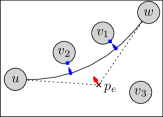
In order to avoid that the edge is curved too much, we also have an attracting force for vertices that have been (almost) intersected by $e$. If $v$ is such a vertex, then the attracting force $F_{\mathrm{ab}}(e,v)=\overrightarrow{p_{e}^{\prime}p_{v}^{\prime}}\cdot d(p_{v}^{\prime},p_{e}^{\prime})^{2}/\sqrt{w_{v}^{2}+h_{v}^{2}}$ is applied to $p_{e}$; see Fig. 3(b).

2.3 Experiments and Evaluation

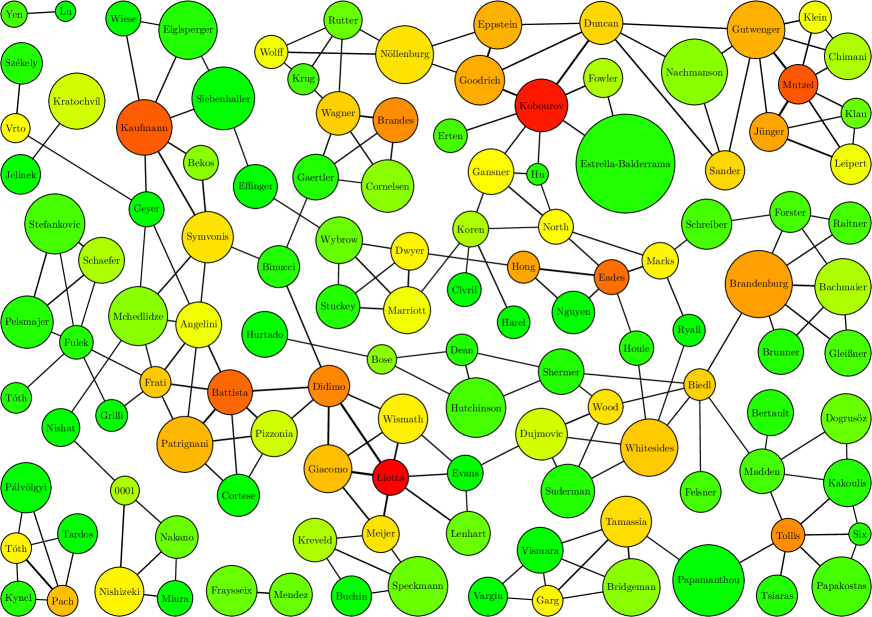
We implemented our heuristic in Java, using the graph library JUNG. Our experiments were performed on a Core i5-2500K CPU with 8 GB of RAM. For the force-directed part of the algorithm, we also used a cooling factor that slows down the movement of vertices over the iterations in order to accelerate the computation of an equilibrium. We configured our algorithm such that there are always 25 steps of shrinking the frame around the current drawing. As input data, we primarily used (subgraphs of) the graph drawing collaboration graph from 1994 till 2012; in total, the graph has 950 vertices and 2559 edges. The weight of each vertex is the number of publications of the respective author and the weight of an edge connecting two authors is the number of their joint publications. We focused on a drawing area of $29.7cm\times 21cm$ (DIN A4) where the size of vertices was determined by the author’s name (in 10pt font). For the complete publication graph, the runtimes were about 2 minutes, depending on the parameters.

The main results of our tests are the following.

• The preprocessing step described in Sec. 2.2 pays off; depending on the parameter $c_{\mathrm{pre}}$, we may save runtime and get better results. In our tests, $c_{\mathrm{pre}}=0.7$ seemed a good choice; see Table 1 in Appendix 0.A.1.

• For testing whether something has to be removed, we set $l_{\mathrm{adj}}=0.1l_{\mathrm{unit}}$ and $l_{\mathrm{nadj}}=0.15l_{\mathrm{unit}}$. For the parameter $c_{\mathrm{len}}$ that determines whether an edge or a vertex will be removed, $c_{\mathrm{len}}=0.9$ gave a good compromise between the vertex and the edge weight in the final drawing; see also Table 2 in Appendix 0.A.1.

• We tested the effect of not always activating the force that repels vertices from edges; instead, we first computed an equilibrium without the force and then another one with it, so that we have more flexibility for vertices to cross edges. In our tests, this proved to have a significant impact on the total weight of edges in the final drawing, yielding an increase of almost 80%; see Table 3 in Appendix 0.A.1.

• The following way of computing the total force vector $F$ for a vertex based on putting weights to the single forces showed the best results: $F=0.01F_{\mathrm{r}}+0.01F_{\mathrm{a}}+0.005F_{\mathrm{g}}+0.0075F_{\mathrm{e}}+0.01F_{\mathrm{f}}$. Note that not all forces are active at the same time.

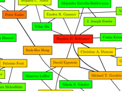
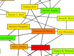
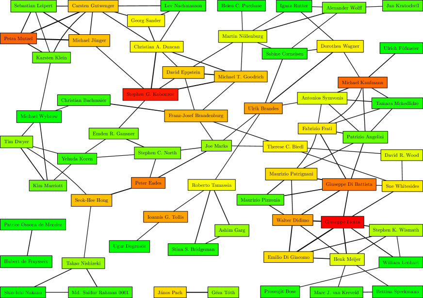
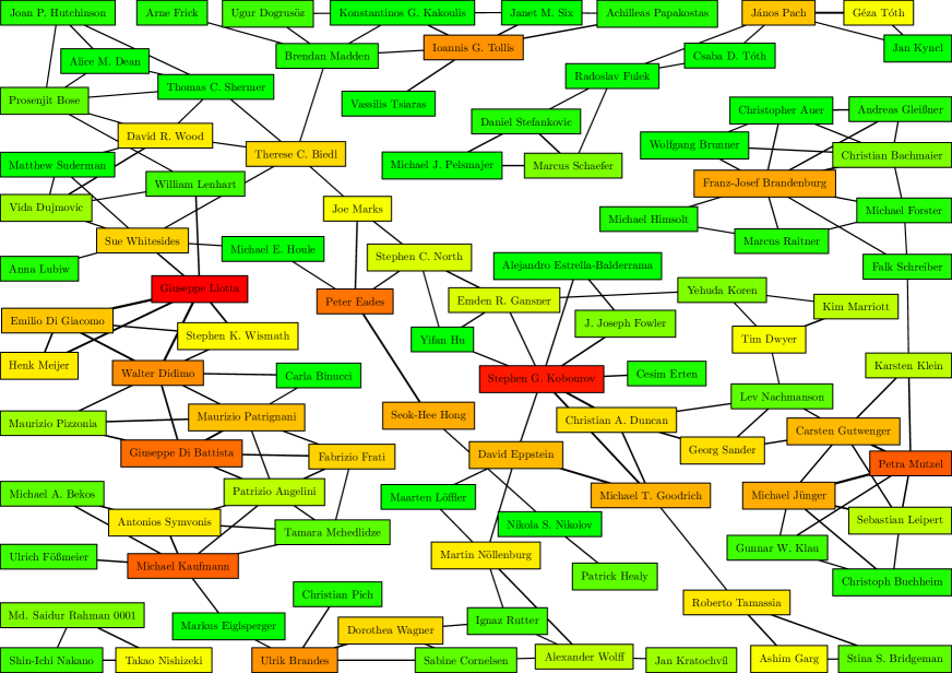
A central parameter used in our algorithm is $l_{\mathrm{unit}}$, describing the desired edge length. Figure 4 shows output examples that demonstrate that higher values lead to drawings that are less dense. Full outputs are attached in Appendix 0.A.2.

(a) Part of an output with $l_{\mathrm{unit}}=2$cm.

(b) Part of an output with $l_{\mathrm{unit}}=3$cm.

Figure 4: Output examples with different choices for $l_{\mathrm{unit}}$.

3 Calculation Graphs

We now consider the initial problem of drawing calculation graphs in prescribed area. In our terminology, most of the input stays the same compared to general graphs, except that now our edges are directed since they represent calculation steps. Additionally, we are given a start vertex $s\in V$ that represents the task given to the students. Hence, $s$ must be present in the output drawing and, furthermore, we insist that in the subgraph that is finally drawn, each vertex can be reached from $s$. To further improve the readability of the steps, we want as many edges as possible pointing from left to right. As a drawing convention for the edges, we will use the orthogonal drawing style with edges leaving vertices horizontally; we try to minimize the numbers of crossings and of bends and to optimize the gaps between edges and vertices. The hardness proof for general graphs can easily be adjusted. Hence, the problem remains NP-hard.

3.1 Our Algorithm

Due to the required readability from left to right, our approach is based on the Sugiyama framework [15] for hierarchical graph drawing. This framework consists of several steps that we will adjust to our problem. Our adjustments are optimized for our drawing style and especially for the task of removing vertices or edges from the graph, if necessary. We first briefly review the steps of the Sugiyama framework before going into detail and describing our adjustments.

In the first step, the graph is made acyclic by reverting some of the edges. Next, the vertices are assigned to layers from left to right. Then, based on the layer assignment, the number of edge crossings is minimized; this step results in relative orders of the vertices of each layer. Eventually, the final coordinates of vertices are computed and the edges are routed.

Breaking the Cycles.

In the later steps of the Sugiyama framework, it is assumed that all edges are directed from left to right, i.e., the graph must be acyclic. To ensure this, we have to revert some edges. If we want to revert the smallest number of edges, we have to solve the NP-hard Feedback Set problem. We can either use existing heuristics, or even afford finding an optimum solution with the help of an MIP solver, which in our tests worked quite fast; this allows us also to minimize the weight of the reverted edges rather than their number.

Layer Assignment.

Several approaches for the layer assignment in the Sugiyama framework exist, depending on the objective, e.g., of minimizing the number of layers or the number of vertices in a layer. Often, the number of layers is minimized subject to a prescribed maximum height of each layer. However, we will not use the height of our drawing area as the maximum height of a layer, although, at first, this may seem a good idea: If we do so, we would most probably have to remove many layers of vertices completely from the graph in later steps, which, subsequently, can also cause the removal of vertices of layers that are not removed, making these layers automatically smaller. Instead, we will set $n_{\mathrm{max}}=\lceil|V|/k\rceil$, where $k$ is the length of the longest path in the graph, so that we can hope for roughly equal numbers of vertices per layer. We mainly used the heuristic of Coffman and Graham [2] with the minor adjustment that preferably the leftmost layers have more vertices; we also tested Graham’s list scheduling algorithm [9] and an assignment with the minimum number of layers.

Vertex Removal.

After the layer assignment, the configuration usually does not fit into the drawing area. We now remove vertices until all vertices can be placed in the drawing area. We first remove vertices from each layer, so that the height of the layer is small enough. Afterwards, we remove whole layers until the width requirement is fulfilled. We first remove single vertices because this step can significantly influence the total weight of layers and, therefore, the choice of layers that will be deleted. The removal from the layers is done from left to right since the removal of a vertex from a layer can cause other vertices right of it to also be removed, if they become unreachable from $s$.

When removing from a layer, we should prefer light vertices. However, we must also take the heights of vertices into account: Removing a high vertex may save as much space as removing several lighter vertices whose weight sums up to a larger value. Hence, we measure the importance of a vertex $v$ as $i(v)=w(v)/h_{v}$ and remove as many vertices of lowest importance as necessary so that the layer fits into the drawing area. We also tried other importance measures by taking the possible decrease of the width of the layer or the decrease of its area into account when removing a vertex. However, these measures did not perform better than the simpler height-based measure.

Once all layers have a feasible height, we will remove complete layers so that we are within the allowed total width. Note that we must always keep gaps between adjacent layers so that the edges can be drawn. The removal of layers is also done from left to right. We do this based on the importance of a layer $L$, which we define as $i(L)=\sum_{v\in L}w(v)/\operatorname{width}(L)$, where the width of $L$ is determined by its widest vertex.

Crossing Minimization.

For the crossing minimization, we use the methods commonly used in the Sugiyama framework, which are based on considering only (parts of) edges between adjacent layers, but do so multiple times. For the adjacent exchange heuristic, we also considered the version where the weight of crossing edges is minimized. This heuristic just performs swaps of adjacent vertices in a layer—if this reduces the number (or weight) of crossings. Hence, weights can easily be integrated.

Edge Removal.

Even after crossing minimization, there could still be too many crossings for the drawing to be well readable, if the graph is dense. Hence, we add a step in which edges are removed, if necessary. To this end, we introduce a measure for the importance of an edge $e$: If $E^{\prime}(e)$ is the set of edges that cross $e$, then the importance of $e$ is $i(e)=w(e)/(\sum_{e^{\prime}\in E^{\prime}(e)}w(e^{\prime}))$. The result is that edges without a crossing are considered most important and will never be removed. Furthermore, an edge that crosses heavy edges—which are more valuable to us—will more likely be removed.

Gaps in Layers.

At this point, we know the orders of vertices in layers, where a layer also includes edges that are routed through several layers. We improve the readability by using different gaps between the objects in a layer: Two edges will be drawn closer together than two vertices, and edges that stay parallel when going to the next layer can be drawn even closer. While the different sizes of gaps make the drawings nicer, the consequence is also that only now we know the precise height each a layer. This can, in some cases, make it necessary to remove another vertex of a layer, which, again, is done based on the importance measure.

Coordinate Assignment.

For the final adjustment of the vertex positions, we still have some flexibility if the vertices (and edges) in the layer do not consume the total available height. We can use this flexibility and try to minimize the number of edge bends. Therefore, we integrated a part of the heuristic of Sander [13]. However, due to the height constraint, we usually cannot save too many bends.

Edge Routing.

Finally, only the edges need to be drawn. There are several subproblems that we will only briefly review:

• We have to distribute the ports of the edges at the incident vertices or use a single port shared by all edges.

• We indicate the weight of edges by drawing them with different width. Since there are only few edges that are very heavy, it makes sense to not use a linear dependency between width and height but, e.g., a logarithmic dependency, or a dependency to the cube root (which gave the nicest results for our drawings).

• We have to distribute the vertical segments of the edges between consecutive layers. We want to do this such that both overlaps between segments and unnecessary (double) crossings are avoided. We first find a relative order of the segments from left to right for each pair of adjacent layers as follows: For any pair of edges between the layers that do not have to cross, there is at most one order with an unnecessary crossing. Using these orders, we build a directed graph of vertical segments. A topological sorting of this graph yields an order of the segments that avoids all unnecessary crossings.

  Once a relative order of the vertical segments is found, we can assign the final coordinates. Several small improvements are possible that locally optimize the spacing between the edge segments and we have put a lot of effort into implementing some of them. The most valuable optimization was the use of a force-directed algorithm with repelling forces between adjacent vertical segments that optimizes the distances between the segments.

3.2 Extensions

Preprocessing.

Similar to our algorithm for general graphs, we use a preprocessing step in which very light vertices and edges are removed in order to speed up the later steps.

Reinsertion of Removed Vertices.

After crossing minimization, when the order of vertices is fixed, it is possible that we could safely reinsert some of the removed vertices so that the available area is used in a better way. We prefer the vertices with the highest importance as defined before and insert them in the leftmost available layer. Note that after reinserting vertices, we may have to reorder some of layers for crossing minimization.

Bézier Curves.

While we try to avoid bends of the orthogonal edges, there still can be longer edges that have several bends, making them hard to follow. We suggest drawing the edges as smooth curves instead. To this end, we represent each edge segment between two adjacent layers as a cubic Bézier curve. As a simple version, this can be done by making the two bends of the orthogonal edge the two middle control points of the curve; this yields already quite nice results. We can further improve the drawings by adjusting the force-directed algorithm for the vertical segments (i.e., the control points): First, we can allow horizontal segments to overlap since they are not actual segments any more. Second, we can add a tendency to put the segments close to the middle between the layers in order to avoid sharp bends. We can, however, not place all vertical segments in the middle; doing so could result in unnecessary crossings of the respective curves.

Weight Transfer.

Suppose we delete a vertex $v$ such that the edges $(u,v)$ and $(v,w)$ for vertices $u$ and $w$ exist. If both edges are heavy, it is possible that many students reached $w$ from $u$ with $v$ as an intermediate step. Hence, after the removal, an edge $(u,w)$ becomes more valuable to us because this edge can also partially represent the steps described above. We can model this by creating edge $(u,w)$—if it did not exist—and increasing its weight by $\min\left\{w(u,v),w(v,w)\right\}$ for the remainder of the algorithm. Similar weight transfers make sense also in more complicated situations.

3.3 Experiments and Evaluation

Also the algorithm for calculation graphs was implemented in Java. We used real-world data generated in user studies, with graphs of 107 and more vertices. The largest graph had 1031 vertices and 1549 edges. As for general graphs, we mainly used the A4 paper size as the prescribed drawing area. The tests were performed on a 3 GHz CPU with 4 GB RAM. Our main results are as follows.

• A preprocessing that removes the lightest vertices often improves the output, i.e., the drawn subgraph is heavier; see Table 4 in Appendix 0.B.1.

• In our tests, there was no significant influence of the choice of the layering algorithm on the final weight of the drawn subgraph, especially when the postprocessing for vertex reinsertion was used.

• The adjacent exchange heuristic for crossing minimization and taking the weight of crossing edges into account reduces the weight of crossing edges significantly (factor $>2$) and causes only few additional crossings; see Table 5 in Appendix 0.B.1.

• The runtime requirement for the largest graph with 1031 vertices was 3 to 4 seconds, depending on the set parameters; the largest part of the time was spent on the force-directed adjustment of segments in the edge routing step and on writing the output file (about 2 seconds).

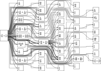
Figure 5 shows an output example using Bézier curves, which, in our opinion, is the nicer and more interesting style compared to the version with orthogonal edges. Full examples can be found in Appendix 0.B.2.

Figure 5: An output example with edges drawn as Bézier curves (scaled down).

4 Conclusion

We have introduced the problem of drawing a heavy subgraph in a prescribed area. Both for general graphs without further constraints and for the special application of calculation graphs, we have developed and tested heuristics which yield quite nice results.

Acknowledgement.

We would like to thank Martin Hennecke for introducing the problem of drawing calculation graphs to us and for providing input data.

Appendix 0.A General Graphs

0.A.1 Pseudocode and Tables

1 compute equilibrium layout;

2 initialize frame $F$ as bounding box around the drawing;

3 while frame $F$ too large do

4       shrink $F$ by constant value;

5       push vertices that are (partially) outside of the frame into $F$;

6       compute new equilibrium layout respecting the boundary of $F$;

7       while min. edge length $<l_{\mathrm{adj}}$ or min. distance of nonadjacent vertices $<l_{\mathrm{nadj}}$ do

8             if average edge length $\leq l_{\mathrm{unit}}\cdot c_{\mathrm{len}}$ then

9                   remove vertex $v$ with maximum stress $s(v)$

10            else

11                   remove edge $e$ with maximum stress $s(e)$

12            

13      compute new equilibrium layout respecting the boundary of $F$;

14      

Algorithm 1 Algorithm for general graphs

$c_{\mathrm{pre}}$	vertices		edges		runtime (s)
	weight	change	weight	change	runtime	change
0.8	659.4	—	716.4	—	111.7	—
0.75	670.4	+ 1.7 %	756.4	+ 5.6 %	135.8	+ 21.6 %
0.7	675.4	+ 2.4 %	769.6	+ 7.4 %	163.2	+ 46.1 %
0.65	668.6	+ 1.4 %	768.0	+ 7.2 %	242.1	+ 116.7 %
0.6	667.8	+ 1.3 %	745.2	+ 4.0 %	708.7	+ 534.5 %

Table 1: Effect of the factor $c_{\mathrm{pre}}$ on runtime and quality of the results for the complete publication graph.

$f_{\text{precision}}$	vertices		edges		runtime (s)
	weight	change	weight	change	runtime	change
0.7	687.7	0	719.0	0	144.4	0
0.8	664.1	– 3.4 %	741.2	+ 3.1 %	149.0	+ 3.2 %
0.9	673.5	– 2.1 %	742.6	+ 3.3 %	127.6	– 11.6 %
1.0	660.7	– 3.9 %	739.6	+ 2.9 %	139.1	– 3.7 %
1.1	628.5	– 8.6 %	705.0	– 1.9 %	133.7	– 7.4 %

Table 2: Effect of the choice of the parameter $c_{\mathrm{len}}$ on runtime and quality of the results for the complete publication graph.

	vertices		edges		runtime (s)
	weight	change	weight	change	runtime	change
1 x equilibrium	663.1	0	412.4	0	107.1	0
2 x equilibrium	666.7	+ 0.5 %	739.6	+ 79.3 %	124.9	+ 16.6 %

Table 3: Improvement in terms of the total edge weight by computing the equilibrium layout always twice, first without and then with the repelling force between vertices and edges.

0.A.2 Output Examples

In our examples, vertex weights are indicated using colors from red (heavy) to green (light).

Figure 6: Example for the complete publication graph with $l_{\mathrm{unit}}=3.0\text{ cm}$; vertices contained in drawing: 6.6 %; vertex weight contained in drawing: 42.1 %; edges contained in drawing: 4.9 %; edge weight contained in drawing: 17.0 %

Figure 7: Example for the complete publication graph with $l_{\mathrm{unit}}=2.0\text{ cm}$; vertices contained in drawing: 10.1 %; vertex weight contained in drawing: 49.4 %; edges contained in drawing: 6.9 %; edge weight contained in drawing: 21.2 %

Figure 8: Same drawing as shown in Fig. 6, but some edges are transformed into quadratic Bézier curves.

Figure 9: Example for the complete publication graph (only last part of the name) with $l_{\mathrm{unit}}=2.0\text{ cm}$; vertices contained in drawing: 12.8 %; vertex weight contained in drawing: 54.2 %; edges contained in drawing: 8.6 %; edge weight contained in drawing: 24.0 %

Appendix 0.B Calculation Graphs

0.B.1 Tables

	vertex weight		edge weight
number of vertices	threshold	improvement	threshold	improvement
107	7	4.49 %	8	7.15 %
143	2	0.45 %	2	0.57 %
170	7	9.21 %	8	14.80 %
203	2	2.24 %	2	3.20 %
331	4	3.32 %	4	6.17 %
358	4	1.92 %	4	3.12 %
406	14	7.12 %	14	11.33 %
530	7	6.49 %	7	11.26 %
563	7	9.32 %	8	16.60 %
663	8	4.96 %	8	9.33 %
755	9	6.76 %	7	9.50 %
775	8	5.02 %	8	7.87 %
799	10	10.35 %	10	17.28 %
1031	11	6.79 %	10	8.64 %

Table 4: Improvement in the vertex and edge weight when activating the preprocessing that removes vertices and edges whose weight is below the given threshold. The table shows results for input graphs of different size.

	vertex weight	edge weight	crossings	weight of crossings
adjacent exchange heuristic	6841.25	6447.48	14.41	3041.54
adjacent exchange with weights	6843.14	6459.70	15.10	1219.68
median heuristic	6845.78	6463.01	13.65	3114.88

Table 5: Comparison of the heuristics for crossing minimization. Resulting values are averages.

0.B.2 Output Examples

Here, we have included some output drawings of calculation graphs, showing different drawing styles for the edges. In Fig. 10, we have orthogonal edges, but only a single port per vertex shared by all outgoing edges. In Fig. 11, the edges are also drawn orthogonally, but now each edge has its own port. Finally, Fig. 11 shows edges that are drawn as Bézier curves. The input graph contained 358 vertices, of which 38 are still contained in Fig. 10, i.e., only 10.6 %. However, these vertices represent 91.1 % of the total vertex weight.

Figure 10: Orthogonal edges with a single port per vertex.

Figure 11: Orthogonal edges with an own port for each outgoing edge.

Figure 12: Edges drawing as Bézier curves; except for the edge style, the drawing is the same as in Fig. 11.

Figure 13: Output drawing for a graph with 203 vertices; contained vertices: 22.1 %; contained vertex weight: 95,2 %; contained edges: 22.0 %; contained edge weight: 94,0 %

Figure 14: Output drawing for a graph with 331 vertices; contained vertices: 13,9 %; contained vertex weight: 92,9 %; contained edges: 11,4 %; contained edge weight: 89,6 %

Figure 15: Output drawing for a graph with 775 vertices; contained vertices: 5,8 %; contained vertex weight: 80,6 %; contained edges: 4,6 %; contained edge weight: 75,0 %

Figure 16: Output drawing for a graph with 799 vertices; contained vertices: 5,4 %; contained vertex weight: 81,7 %; contained edges: 5,3 %; contained edge weight: 78,7 %

Figure 17: Output drawing for a graph with 1031 vertices; contained vertices: 4,7 %; contained vertex weight: 75,9 %; contained edges: 4,1 %; contained edge weight: 74,1 %

Figure 18: Output drawing for a graph with 1031 vertices; no crossings are allowed; contained vertices: 4,3 %; contained vertex weight: 76,6 %; contained edges: 3,9 %; contained edge weight: 70,2 %

References

- [1] Bertault, F.: A force-directed algorithm that preserves edge crossing properties. Inf. Proc. Letters 74(1–2), 7–13 (2000)
- [2] Coffman, E.G., Graham, R.L.: Optimal scheduling for two-processor systems. Acta Informatica 1(3), 200–213 (1972)
- [3] Da Lozzo, G., Di Battista, G., Ingrassia, F.: Drawing graphs on a smartphone. J. Graph Algorithms Appl. 16(1), 109–126 (2012)
- [4] Duncan, C., Gutwenger, C., Nachmanson, L., Sander, G.: Graph drawing contest report. In: Didimo, W., Patrignani, M. (eds.) Proc. 20th Int. Symp. Graph Drawing (GD’12), LNCS, vol. 7704, pp. 575–579. Springer, Heidelberg (2013)
- [5] Dwyer, T., Marriott, K., Schreiber, F., Stuckey, P., Woodward, M., Wybrow, M.: Exploration of networks using overview+detail with constraint-based cooperative layout. IEEE Trans. Vis. Comput. Graph. 14(6), 1293–1300 (2008)
- [6] Dwyer, T., Koren, Y., Marriott, K.: IPSep-CoLa: An incremental procedure for separation constraint layout of graphs. IEEE Trans. Vis. Comput. Graph. 12(5), 821–828 (2006)
- [7] Dwyer, T., Marriott, K., Wybrow, M.: Topology preserving constrained graph layout. In: Tollis, I.G., Patrignani, M. (eds.) Proc. 16th Int. Symp. Graph Drawing (GD’08), LNCS, vol. 5417, pp. 230–241. Springer, Heidelberg (2009)
- [8] Fruchterman, T.M.J., Reingold, E.M.: Graph drawing by force-directed placement. Software: Practice and Experience 21(11), 1129–1164 (1991)
- [9] Graham, R.L.: Bounds for certain multiprocessing anomalies. The Bell System Technical Journal 45(9), 1563–1581 (1966)
- [10] He, W., Marriott, K.: Constrained graph layout. Constraints 3(4), 289–314 (1998)
- [11] Hennecke, M.: Rechengraphen. mathematica didactica 1, 68–96 (2007)
- [12] Patrignani, M.: On the complexity of orthogonal compaction. Computational Geometry 19(1), 47–67 (2001)
- [13] Sander, G.: A fast heuristic for hierarchical manhattan layout. In: Brandenburg, F.J. (ed.) Proc. Symp. Graph Drawing (GD ’95), LNCS, vol. 1027, pp. 447–458. Springer, Heidelberg (1996)
- [14] Simonetto, P., Archambault, D., Auber, D., Bourqui, R.: ImPrEd: An improved force-directed algorithm that prevents nodes from crossing edges. Computer Graphics Forum 30(3), 1071–1080 (2011)
- [15] Sugiyama, K., Tagawa, S., Toda, M.: Methods for visual understanding of hierarchical system structures. IEEE Transactions on Systems, Man and Cybernetics 11(2), 109–125 (1981)