Google matrix analysis of directed networks

Abstract

In the past decade modern societies have developed enormous communication and social networks. Their classification and information retrieval processing has become a formidable task for the society. Due to the rapid growth of the World Wide Web, and social and communication networks, new mathematical methods have been invented to characterize the properties of these networks in a more detailed and precise way. Various search engines use extensively such methods. It is highly important to develop new tools to classify and rank massive amount of network information in a way that is adapted to internal network structures and characteristics. This review describes the Google matrix analysis of directed complex networks demonstrating its efficiency using various examples including World Wide Web, Wikipedia, software architectures, world trade, social and citation networks, brain neural networks, DNA sequences and Ulam networks. The analytical and numerical matrix methods used in this analysis originate from the fields of Markov chains, quantum chaos and Random Matrix theory.

“The Library exists ab aeterno.”
Jorge Luis Borges The Library of Babel

I Introduction

In the past ten years, modern societies have developed enormous communication and social networks. The World Wide Web (WWW) alone has about 50 billion indexed web pages, so that their classification and information retrieval processing becomes a formidable task. Various search engines have been developed by private companies such as Google, Yahoo! and others which are extensively used by Internet users. In addition, social networks (Facebook, LiveJournal, Twitter, etc) have gained huge popularity in the last few years. In addition, use of social networks has spread beyond their initial purpose, making them important for political or social events.

To handle such massive databases, fundamental mathematical tools and algorithms related to centrality measures and network matrix properties are actively being developed. Indeed, the PageRank algorithm, which was initially at the basis of the development of the Google search engine Brin and Page (1998); Langville and Meyer (2006), is directly linked to the mathematical properties of Markov chains Markov (1906) and Perron-Frobenius operators Brin and Stuck (2002); Langville and Meyer (2006). Due to its mathematical foundation, this algorithm determines a ranking order of nodes that can be applied to various types of directed networks. However, the recent rapid development of WWW and communication networks requires the creation of new tools and algorithms to characterize the properties of these networks on a more detailed and precise level. For example, such networks contain weakly coupled or secret communities which may correspond to very small values of the PageRank and are hard to detect. It is therefore highly important to have new methods to classify and rank hige amounts of network information in a way adapted to internal network structures and characteristics.

This review describes matrix tools and algorithms which facilitate classification and information retrieval from large networks recently created by human activity. The Google matrix, formed by links of the network has, is typically huge (a few tens of billions of webpages). Thus, the analysis of its spectral properties including complex eigenvalues and eigenvectors represents a challenge for analytical and numerical methods. It is rather surprising, but the class of such matrices, which belong to the class of Markov chains and Perron-Frobenius operators, has been essentially overlooked in physics. Indeed, physical problems typically belong to the class of Hermitian or unitary matrices. Their properties have been actively studied in the frame of Random Matrix Theory (RMT) Akemann et al. (2011); Guhr et al. (1998); Mehta (2004) and quantum chaos Haake (2010). The analytical and numerical tools developed in these research fields have paved the way for understanding many universal and peculiar features of such matrices in the limit of large matrix size corresponding to many-body quantum systems Guhr et al. (1998), quantum computers Shepelyansky (2001) and a semiclassical limit of large quantum numbers in the regime of quantum chaos Haake (2010). In contrast to the Hermitian problem, the Google matrices of directed networks have complex eigenvalues. The only physical systems where similar matrices had been studied analytically and numerically correspond to models of quantum chaotic scattering whose spectrum is known to have such unusual properties as the fractal Weyl law Gaspard (2014); Sjöstrand (1990); Nonnenmacher and Zworski (2007); Shepelyansky (2008); Zworski (1999).

Figure 1: (Color online) Google matrix of the network Wikipedia English articles for Aug 2009 in the basis of PageRank index $K$ (and $K^{\prime}$). Matrix $G_{KK^{\prime}}$ corresponds to $x$ (and $y$) axis with $1\leq K,K^{\prime}\leq 200$ on panel (a), and with $1\leq K,K^{\prime}\leq N$ on panel (b); all nodes are ordered by PageRank index $K$ of matrix $G$ and thus we have two matrix indexes $K,K^{\prime}$ for matrix elements in this basis. Panel (a) shows the first $200\times 200$ matrix elements of $G$ matrix (see Sec. III). Panel (b) shows density of all matrix elements coarse-grained on $500\times 500$ cells where its elements, $G_{K,K^{\prime}}$, are written in the PageRank basis $K(i)$ with indexes $i\rightarrow K(i)$ (in $x$-axis) and $j\rightarrow K^{\prime}(j)$ (in a usual matrix representation with $K=K^{\prime}=1$ on the top-left corner). Color shows the density of matrix elements changing from black for minimum value ($(1-\alpha)/N$) to white for maximum value via green (gray) and yellow (light gray); here the damping factor is $\alpha=0.85$ After Ermann et al. (2012a).

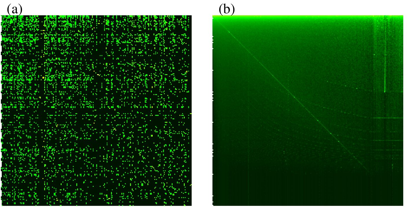
In this review we present an extensive analysis of a variety of Google matrices emerging from real networks in various sciences including WWW of UK universities, Wikipedia, Physical Review citation network, Linux Kernel network, world trade network from the UN COMTRADE database, brain neural networks, networks of DNA sequences and many others. As an example, the Google matrix of the Wikipedia network of English articles (2009) is shown in Fig. 1. We demonstrate that the analysis of the spectrum and eigenstates of a Google matrix of a given network provides a detailed understanding about the information flow and ranking. We also show that such types of matrices naturally appear for Ulam networks of dynamical maps Frahm and Shepelyansky (2012b); Shepelyansky and Zhirov (2010a) in the framework of the Ulam method Ulam (1960).

Currently, Wikipedia, a free online encyclopaedia, stores more and more information and has become the largest database of human knowledge. In this respect it is similar to the Library of Babel, described by Jorge Luis Borges Borges (1962). The understanding of hidden relations between various areas of knowledge on the basis of Wikipedia can be improved with the help of Google matrix analysis of directed hyperlink networks of Wikipedia articles as described in this review.

The specific tools of RMT and quantum chaos, combined with the efficient numerical methods for large matrix diagonalization like the Arnoldi method Stewart (2001), allow to analyze the spectral properties of such large matrices as the entire Twitter network of 41 millions users Frahm and Shepelyansky (2012b). In 1998 Brin and Page pointed out that “despite the importance of large-scale search engines on the web, very little academic research has been done on them” Brin and Page (1998). The Google matrix of a directed network, like the Library of Babel of Borges Borges (1962), contains all the information about a network. The PageRank eigenvector of this matrix finds a broad range of applications being at the mathematical foundations of the Google search engine Brin and Page (1998); Langville and Meyer (2006). We show below that the spectrum of this matrix and its other eigenvectors also provide interesting information about network communities and the formation of PageRank vector. We hope that this review yields a solid scientific basis of matrix methods for efficient analysis of directed networks emerging in various sciences. The described methods will find broad interdisciplinary applications in mathematics, physics and computer science with the cross-fertilization of different research fields. Our aim is to combine the analytic tools and numerical analysis of concrete directed networks to gain a better understanding of the properties of these complex systems.

An interested reader can find a general introduction about complex networks (see also Sec. II) in well established papers, reviews and books Watts and Strogatz (1998), Albert and Barabási (2002); Caldarelli (2003); Newman (2003), Dorogovtsev et al. (2008); Castellano et al. (2009), Dorogovtsev (2010); Fortunato (2010); Newman (2010). Descriptions of Markov chains and Perron-Frobenius operators are given in Brin and Page (1998); Brin and Stuck (2002); Gantmacher (2000); Langville and Meyer (2006), while the properties of Random Matrix Theory (RMT) and quantum chaos are described in Akemann et al. (2011); Haake (2010); Guhr et al. (1998); Mehta (2004).

The data sets for the main part of the networks considered here are available at FETNADINE database (2014) from Quantware group.

II Scale-free properties of directed networks

The distributions of the number of ingoing or outgoing links per node for directed networks with $N$ nodes and $N_{\ell}$ links are well known as indegree and outdegree distributions in the community of computer science Caldarelli (2003); Donato et al. (2004); Pandurangan et al. (2005). A network is described by an adjacency matrix $A_{ij}$ of size $N\times N$ with $A_{ij}=1$ when there is a link from a node $j$ to a node $i$ in the network, i. e. “$j$ points to $i$”, and $A_{ij}=0$ otherwise. Real networks are often characterized by power law distributions for the number of ingoing and outgoing links per node $w_{\rm in,out}(k)\propto 1/k^{\mu_{\rm in,out}}$ with typical exponents $\mu_{\rm in}\approx 2.1$ and $\mu_{\rm out}\approx 2.7$ for the WWW. For example, for the Wikipedia network of Fig. 1 one finds $\mu_{\rm in}=2.09\pm 0.04$, $\mu_{\rm out}=2.76\pm 0.06$ as shown in Fig. 2 Zhirov et al. (2010).

Figure 2: (Color online) Distribution $w_{\rm in,out}(k)$ of number of ingoing (a) and outgoing (b) links $k$ for $N=3282257$ Wikipedia English articles (Aug 2009) of Fig. 1 with total number of links $N_{\ell}=71012307$. The straight dashed fit line shows the slope with $\mu_{\rm in}=2.09\pm 0.04$ (a) and $\mu_{\rm out}=2.76\pm 0.06$ (b). After Zhirov et al. (2010).

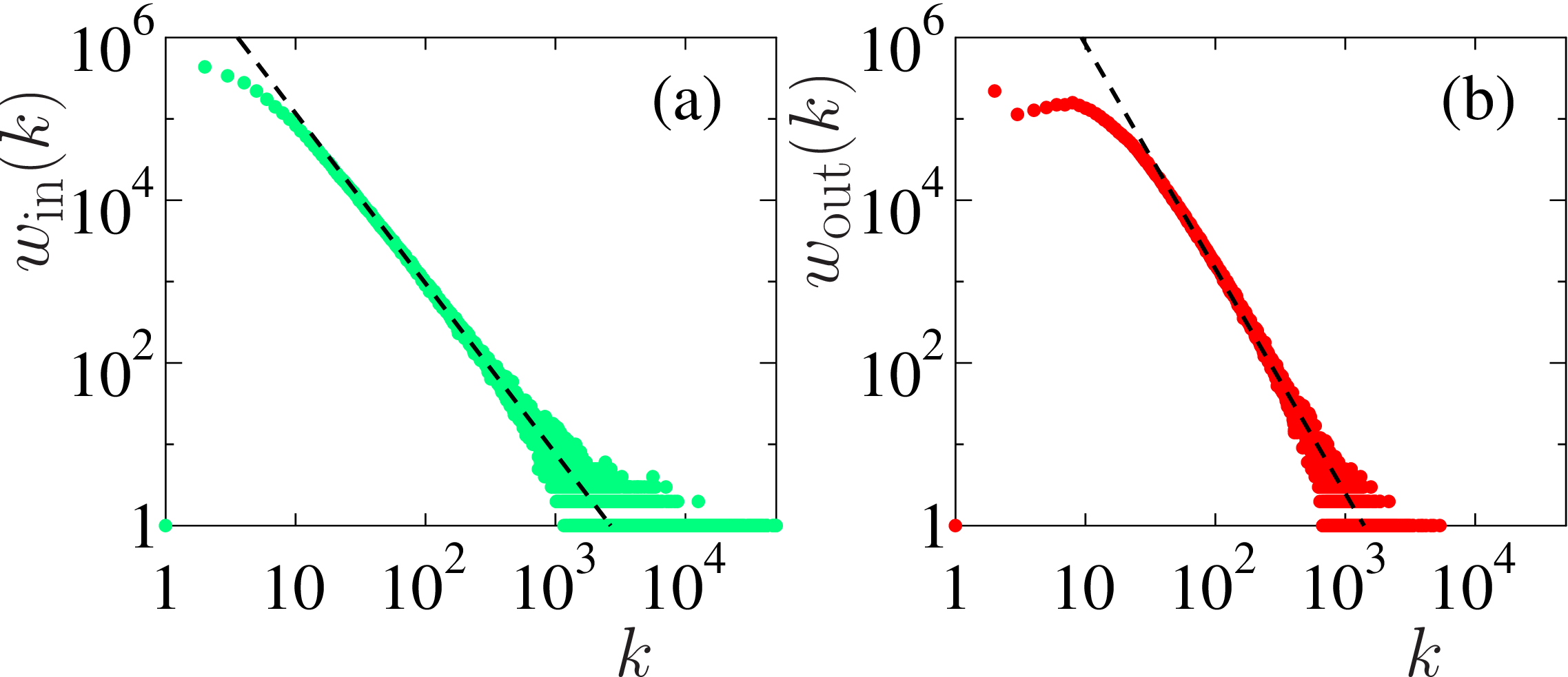
Statistical preferential attachment models were initially developed for undirected networks Albert and Barabási (2000). Their generalization to directed networks Giraud et al. (2009) generates a power law distribution for ingoing links with $\mu_{\rm in}\approx 2$ but the distribution of outgoing links is closer to an exponential decay. We will see below that these models are not able to reproduce the spectral properties of $G$ in real networks.

The most recent studies of WWW, crawled by the Common Crawl Foundation in 2012 Meusel et al. (2014) for $N\approx 3.5\times 10^{9}$ nodes and $N_{\ell}\approx 1.29\times 10^{11}$ links, provide the exponents $\mu_{\rm in}\approx 2.24$, $\mu_{\rm out}\approx 2.77$, even if the authors stress that these distributions describe probabilities at the tails which capture only about one percent of nodes. Thus, at present the existing statistical models of networks capture only in an approximate manner the real situation in large networks even if certain models are able to generate a power law decay of PageRank probability.

III Construction of Google matrix and its properties

III.1 Construction rules

The matrix $S_{ij}$ of Markov transitions Markov (1906) is constructed from the adjacency matrix $A_{ij}\rightarrow S_{ij}$ by normalizing elements of each column so that their sum is equal to unity ($\sum_{i}S_{ij}=1$) and replacing columns with only zero elements (dangling nodes) by $1/N$. Such matrices with columns sum normalized to unity and $S_{ij}\geq 0$ belong to the class of Perron-Frobenius operators with a possibly degenerate unit eigenvalue $\lambda=1$ and other eigenvalues obeying $|\lambda|\leq 1$ (see Sec. III.2). Then the Google matrix of the network is introduced as: Brin and Page (1998)

$$G_{ij}=\alpha S_{ij}+(1-\alpha)/N\;\;.$$ (1)

The damping factor $\alpha$ in the WWW context describes the probability $(1-\alpha)$ to jump to any node for a random surfer. At a given node a random surfer follows the available direction of links making a random choice between them with probability proportional to the weight of links. For WWW the Google search engine uses $\alpha\approx 0.85$ Langville and Meyer (2006). For $0\leq\alpha\leq 1$ the matrix $G$ also belongs to the class of Perron-Frobenius operators as $S$ and with its columns sum normalized. However, for $\alpha<1$ its largest eigenvalue $\lambda=1$ is not degenerate and the other eigenvalues lie inside a smaller circle of radius $\alpha$, i.e. $|\lambda|\leq\alpha$ Brin and Stuck (2002); Langville and Meyer (2006).

Figure 3: (Color online) (a) Example of simple network with directed links between 5 nodes. (b) Distribution of 5 nodes from (a) on the PageRank-CheiRank plane $(K,K^{*})$, where the size of node is proportional to PageRank probability $P(K)$ and color of node is proportional to CheiRank probability $P^{*}(K^{*})$, with maximum at red/gray and minimum at blue/black; the location of nodes of panel (a) on $(K_{i},{K_{i}}^{*})$ plane is: $(2,4)$, $(1,3)$, $(3,1)$, $(4,2)$, $(5,5)$ for original nodes $i=1,2,3,4,5$ respectively; PageRank and CheiRank vectors are computed from the Google matrices $G$ and $G^{*}$ shown in Fig. 4 at a damping factor $\alpha=0.85$.

The right eigenvector at $\lambda=1$, which is called the PageRank, has real nonnegative elements $P(i)$ and gives the stationary probability $P(i)$ to find a random surfer at site $i$. The PageRank can be efficiently determined by the power iteration method which consists of repeatedly multiplying $G$ to an iteration vector which is initially chosen as a given random or uniform initial vector. Developing the initial vector in a basis of eigenvectors of $G$ one finds that the other eigenvector coefficients decay as $\sim\lambda^{n}$ and only the PageRank component, with $\lambda=1$, survives in the limit $n\to\infty$. The finite gap $1-\alpha\approx 0.15$ between the largest eigenvalue and other eigenvalues ensures, after several tens of iterations, the fast exponential convergence of the method also called the “PageRank algorithm”. A multiplication of $G$ to a vector requires only $O(N_{\ell})$ multiplications due to the links and the additional contributions due to dangling nodes and damping factor can be efficiently performed with $O(N)$ operations. Since often the average number of links per node is of the order of a few tens for WWW and many other networks one has effectively $N_{\ell}$ and $N$ of the same order of magnitude. At $\alpha=1$ the matrix $G$ coincides with the matrix $S$ and we will see below in Sec. VIII that for this case the largest eigenvalue $\lambda=1$ is usually highly degenerate due to many invariant subspaces which define many independent Perron-Frobenius operators with at least one eigenvalue $\lambda=1$ for each of them.

Once the PageRank is found, e.g. at $\alpha=0.85$, all nodes can be sorted by decreasing probabilities $P(i)$. The node rank is then given by the index $K(i)$ which reflects the relevance of the node $i$. The top PageRank nodes, with largest probabilities, are located at small values of $K(i)=1,2,...$.

It is known that on average the PageRank probability is proportional to the number of ingoing links Langville and Meyer (2006); Litvak et al. (2008), characterizing how popular or known a given node is. Assuming that the PageRank probability decays algebraically as $P_{i}\sim 1/K_{i}^{\beta}$ we obtain that the number of nodes $N_{P}$ with PageRank probability $P$ scales as $N_{P}\sim 1/P^{\mu_{\rm in}}$ with $\mu_{\rm in}=1+1/\beta$ so that $\beta\approx 0.9$ for $\mu_{\rm in}\approx 2.1$ being in a agreement with the numerical data for WWW Donato et al. (2004); Pandurangan et al. (2005); Meusel et al. (2014) and Wikipedia network Zhirov et al. (2010). More recent mathematical studies on the relation between PageRank probability decay and ingoing links are reported in Jelenkovic and Olvera-Cravioto (2013); Chen et al. (2014). At the same time the proportionality relation between PageRank probability and ingoing links assumes certain statistical properties of networks and works only on average. We note that there are examples of Ulam networks generated by dynamical maps where such proportionality is not working (see Ermann and Shepelyansky (2010a) and Sec. VI.5).

In addition to a given directed network with adjacency matrix $A$ it is useful to analyze an inverse network where links are inverted and whose adjacency matrix $A^{*}$ is the transpose of $A$, i.e. $A^{*}_{ij}=A_{ji}$. The matrices $S^{*}$ and the Google matrix $G^{*}$ of the inverse network are then constructed in the same way from $A^{*}$ as described above and according to the relation (1) using the same value of $\alpha$ as for the $G$ matrix. The right eigenvector of $G^{*}$ at eigenvalue $\lambda=1$ is called CheiRank giving a complementary rank index $K^{*}(i)$ of network nodes Chepelianskii (2010); Zhirov et al. (2010); Ermann et al. (2012a). The CheiRank probability $P^{*}(K^{*})$ is proportional to the number of outgoing links highlighting node communicativity (see e.g. Ermann et al. (2012a); Zhirov et al. (2010)). In analogy with the PageRank we obtain that $P^{*}\sim 1/{{K^{*}}^{\beta}}$ with $\beta=1/(\mu_{\rm out}-1)\approx 0.6$ for typical $\mu_{\rm out}\approx 2.7$. The statistical properties of distribution of nodes on the PageRank-CheiRank plane are described in Ermann et al. (2012a) for various directed networks. We will discuss them below.

Figure 4: (a) Adjacency matrix $A$ of network of Fig. 3(a) with indexes used there, (b) adjacency matrix $A^{*}$ for the network with inverted links; matrices $S$ (c) and $S^{*}$ (d) corresponding to the matrices $A$, $A^{*}$; the Google matrices $G$ (e) and $G^{*}$ (f) corresponding to matrices $S$ and $S^{*}$ for $\alpha=0.85$ (only 3 digits of matrix elements are shown).

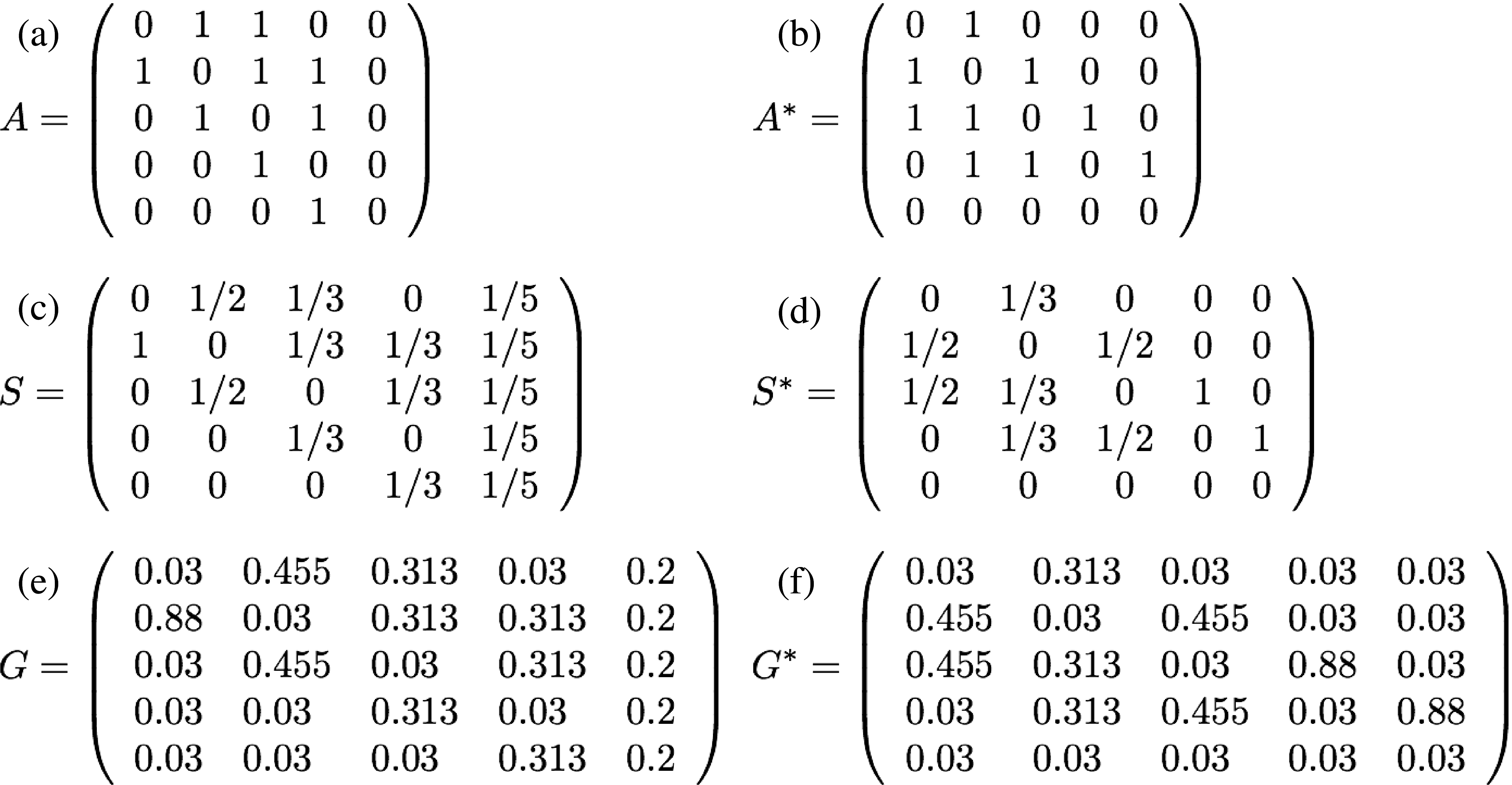
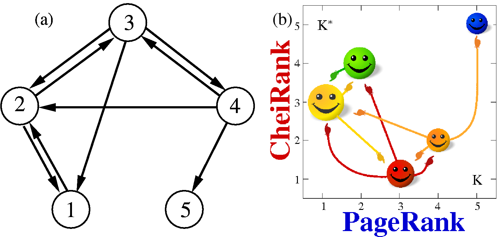
For an illustration we consider an example of a simple network of five nodes shown in Fig. 3(a). The corresponding adjacency matrices $A$, $A^{*}$ are shown in Fig. 4 for the indexes given in Fig. 3(a). The matrices of Markov transitions $S$, $S^{*}$ and Google matrices are computed as described above and from Eq. (1). The distribution of nodes on $(K,K^{*})$ plane is shown in Fig. 3(b). After permutations the matrix $G$ can be rewritten in the basis of PageRank index $K$ as it is done in Fig. 1.

III.2 Markov chains and Perron-Frobenius operators

Matrices with real non-negative elements and column sums normalized to unity belong to the class of Markov chains Markov (1906) and Perron-Frobenius operators Brin and Stuck (2002); Gantmacher (2000); Langville and Meyer (2006), which have been used in a mathematical analysis of dynamical systems and theory of matrices. A numerical analysis of finite size approximants of such operators is closely linked with the Ulam method Ulam (1960) which naturally generates such matrices for dynamical maps Ermann and Shepelyansky (2010a, b); Shepelyansky and Zhirov (2010a). The Ulam method generates Ulam networks whose properties are discussed in Sec.VI.

Matrices $G$ of this type have at least (one) unit eigenvalue $\lambda=1$ since the vector $e^{T}=(1,\,\ldots,\,1)$ is obviously a left eigenvector for this eigenvalue. Furthermore one verifies easily that for any vector $v$ the inequality $\|G\,v\|_{1}\leq\|v\|_{1}$ holds where the norm is the standard 1-norm. From this inequality one obtains immediately that all eigenvalues $\lambda$ of $G$ lie in a circle of radius unity: $|\lambda|\leq 1$. For the Google matrix $G$ as given in (1) one can furthermore show for $\alpha<1$ that the unity eigenvalue is not degenerate and the other eigenvalues obey even $|\lambda|\leq\alpha$ Langville and Meyer (2006). These and other mathematical results about properties of matrices of such type can be found at Gantmacher (2000); Langville and Meyer (2006).

It should be pointed out that due to the asymmetry of links on directed networks such matrices have in general a complex eigenvalue spectrum and sometimes they are not even diagonalizable, i.e. there may also be generalized eigenvectors associated to non-trivial Jordan blocks. Matrices of this type rarely appear in physical problems which are usually characterized by Hermitian or unitary matrices with real eigenvalues or located on the unitary circle. The universal spectral properties of such hermitian or unitary matrices are well described by RMT Akemann et al. (2011); Haake (2010); Guhr et al. (1998). In contrast to this non-trivial complex spectra appear in physical systems only in problems of quantum chaotic scattering and systems with absorption. In such cases it may happen that the number of states $N_{\gamma}$, with finite values $0<\lambda_{\rm min}\leq|\lambda|\leq 1$ ($\gamma=-2\ln|\lambda|$), can grow algebraically $N_{\gamma}\propto N^{\nu}$ with increasing matrix size $N$, with an exponent $\nu<1$ corresponding to a fractal Weyl law proposed first in mathematics Sjöstrand (1990). Therefore most of eigenvalues drop to $\lambda=0$ with $N\to\infty$. We discuss this unusual property in Sec.V.

III.3 Invariant subspaces

For typical networks the set of nodes can be decomposed in invariant subspace nodes and fully connected core space nodes leading to a block structure of the matrix $S$ in (1) which can be represented as Frahm et al. (2011):

$$S=\left(\begin{array}[]{cc}S_{ss}&S_{sc}\\ 0&S_{cc}\\ \end{array}\right)\;.$$ (2)

The core space block $S_{cc}$ contains the links between core space nodes and the coupling block $S_{sc}$ may contain links from certain core space nodes to certain invariant subspace nodes. By construction there are no links from nodes of invariant subspaces to the nodes of core space. Thus the subspace-subspace block $S_{ss}$ is actually composed of many diagonal blocks for many invariant subspaces whose number can generally be rather large. Each of these blocks corresponds to a column sum normalized matrix with positive elements of the same type as $G$ and has therefore at least one unit eigenvalue. This leads to a high degeneracy $N_{1}$ of the eigenvalue $\lambda=1$ of $S$, for example $N_{1}\sim 10^{3}$ as for the case of UK universities (see Sec. VIII).

In order to obtain the invariant subspaces, we determine iteratively for each node the set of nodes that can be reached by a chain of non-zero matrix elements of $S$. If this set contains all nodes (or at least a macroscopic fraction) of the network, the initial node belongs to the core space $V_{c}$. Otherwise, the limit set defines a subspace which is invariant with respect to applications of the matrix $S$. At a second step all subspaces with common members are merged resulting in a sequence of disjoint subspaces $V_{j}$ of dimension $d_{j}$ and which are invariant by applications of $S$. This scheme, which can be efficiently implemented in a computer program, provides a subdivision over $N_{c}$ core space nodes (70-80% of $N$ for UK university networks) and $N_{s}=N-N_{c}$ subspace nodes belonging to at least one of the invariant subspaces $V_{j}$. This procedure generates the block triangular structure (2). One may note that since a dangling node is connected by construction to all other nodes it belongs obviously to the core space as well as all nodes which are linked (directly or indirectly) to a dangling node. As a consequence the invariant subspaces do not contain dangling nodes nor nodes linked to dangling nodes.

The detailed algorithm for an efficient computation of the invariant subspaces is described in Frahm et al. (2011). As a result the total number of all subspace nodes $N_{s}$, the number of independent subspaces $N_{d}$, the maximal subspace dimension $d_{\rm max}$ etc. can be determined. The statistical properties for the distribution of subspace dimensions are discussed in Sec. VIII for UK universities and Wikipedia networks. Furthermore it is possible to determine numerically with a very low effort the eigenvalues of $S$ associated to each subspace by separate diagonalization of the corresponding diagonal blocks in the matrix $S_{ss}$. For this, either exact diagonalization or, in rare cases of quite large subspaces, the Arnoldi method (see the next subsection) can be used.

After the subspace eigenvalues are determined one can apply the Arnoldi method to the projected core space matrix block $S_{cc}$ to determine the leading core space eigenvalues. In this way one obtains accurate eigenvalues because the Arnoldi method does not need to compute the numerically very problematic highly degenerate unit eigenvalues of $S$ since the latter are already obtained from the separate and cheap subspace diagonalization. Actually the alternative and naive application of the Arnoldi method on the full matrix $S$, without computing the subspaces first, does not provide the correct number $N_{1}$ of degenerate unit eigenvalues and also the obtained clustered eigenvalues, close to unity, are not very accurate. Similar problems hold for the full matrix $G$ (with damping factor $\alpha<1$) since here only the first eigenvector, the PageRank, can be determined accurately but there are still many degenerate (or clustered) eigenvalues at (or close to) $\lambda=\alpha$.

Since the columns sums of $S_{cc}$ are less than unity, due to non-zero matrix elements in the block $S_{sc}$, the leading core space eigenvalue of $S_{cc}$ is also below unity $|\lambda_{1}^{(\rm core)}|<1$ even though in certain cases the gap to unity may be very small (see Sec. VIII).

We consider concrete examples of such decompositions in Sec. VIII and show in this review spectra with subspace and core space eigenvalues of matrices $S$ for several network examples. The mathematical results for properties of the matrix $S$ are discussed in Serra-Capizzano (2005).

III.4 Arnoldi method for numerical diagonalization

The most adapted numerical method to determine the largest eigenvalues of large sparse matrices is the Arnoldi method Arnoldi (1951); Frahm and Shepelyansky (2010); Golub and Greif (2006); Stewart (2001). Indeed, usually the matrix $S$ in Eq. (1) is very sparse with only a few tens of links per node $\zeta=N_{\ell}/N\sim 10$. Thus, a multiplication of a vector by $G$ or $S$ is numerically cheap. The Arnoldi method is similar in spirit to the Lanzcos method, but is adapted to non-Hermitian or non-symmetric matrices. Its main idea is to determine recursively an orthonormal set of vectors $\xi_{0},\,\ldots\,\xi_{n_{\rm A}-1}$, which define a Krylov space, by orthogonalizing $S\xi_{k}$ on the previous vectors $\xi_{0},\,\ldots\xi_{k}$ by the Gram-Schmidt procedure to obtain $\xi_{k+1}$ and where $\xi_{0}$ is some normalized initial vector. The dimension $n_{\rm A}$ of the Krylov space (in the following called the Arnoldi-dimension) should be “modest” but not too small. During the Gram-Schmidt procedure one obtains furthermore the explicit expression: $S\xi_{k}=\sum_{j=0}^{k+1}h_{jk}\,\xi_{j}$ with matrix elements $h_{jk}$, of the Arnoldi representation matrix of $S$ on the Krylov space, given by the scalar products or inverse normalization constants calculated during the orthogonalization. In order to obtain a closed representation matrix one needs to replace the last coupling element $h_{n_{\rm A},n_{\rm A}-1}\to 0$ which introduces a mathematical approximation. The eigenvalues of the $n_{\rm A}\times n_{\rm A}$ matrix $h$ are called the Ritz eigenvalues and represent often very accurate approximations of the exact eigenvalues of $S$, at least for a considerable fraction of the Ritz eigenvalues with largest modulus.

In certain particular cases, when $\xi_{0}$ belongs to an $S$ invariant subspace of small dimension $d$, the element $h_{d,d-1}$ vanishes automatically (if $d\leq n_{\rm A}$ and assuming that numerical rounding errors are not important) and the Arnoldi iteration stops at $k=d$ and provides $d$ exact eigenvalues of $S$ for the invariant subspace. One can mention that there are more sophisticated variants of the Arnoldi method Stewart (2001) where one applies (implicit) modifications on the initial vector $\xi_{0}$ in order to force this vector to be in some small dimensional invariant subspace which results in such a vanishing coupling matrix element. These variants known as (implicitly) restarted Arnoldi methods allow to concentrate on certain regions on the complex plane to determine a few but very accurate eigenvalues in these regions. However, for the cases of Google matrices, where one is typically interested in the largest eigenvalues close to the unit circle, only the basic variant described above was used but choosing larger values of $n_{\rm A}$ as would have been possible with the restarted variants. The initial vector was typically chosen to be random or as the vector with unit entries.

Concerning the numerical resources the Arnoldi method requires $\zeta N$ double precision registers to store the non-zero matrix elements of $S$, $n_{\rm A}N$ registers to store the vectors $\xi_{k}$ and const.$\times n_{\rm A}^{2}$ registers to store $h$ (and various copies of $h$). The computational time scales as $\zeta\,n_{\rm A}\,N_{d}$ for the computation of $S\,\xi_{k}$, with $N_{d}\,n_{\rm A}^{2}$ for the Gram-Schmidt orthogonalization procedure (which is typically dominant) and with const.$\times n_{\rm A}^{3}$ for the diagonalization of $h$.

The details of the Arnoldi method are described in Refs. given above. This method has problems with degenerate or strongly clustered eigenvalues and therefore for typical examples of Google matrices it is applied to the core space block $S_{cc}$ where the effects of the invariant subspaces, being responsible for most of the degeneracies, are exactly taken out according to the discussion of the previous subsection. In typical examples it is possible to find about $n_{\rm A}\approx 640$ eigenvalues with largest $|\lambda|$ for the entire Twitter network with $N\approx 4.1\times 10^{7}$ (see Sec. X) and about $n_{\rm A}\approx 6000$ eigenvalues for Wikipedia networks with $N\approx 3.2\times 10^{6}$ (see Sec. IX). For the two university networks of Cambridge and Oxford 2006 with $N\approx 2\times 10^{5}$ it is possible to compute $n_{\rm A}\approx 20000$ eigenvalues (see Sec. VIII). For the case of the Citation network of Physical Review (see Sec. XII) with $N\approx 4.6\times 10^{5}$ it is even possible and necessary to use high precision computations (with up to 768 binary digits) to determine accurately the Arnoldi matrix $h$ with $n_{\rm A}\approx 2000$ Frahm et al. (2014b).

III.5 General properties of eigenvalues and eigenstates

According to the Perron-Frobenius theorem all eigenvalues $\lambda_{i}$ of $G$ are distributed inside the unitary circle $|\lambda|\leq 1$. It can be shown that at $\alpha<1$ there is only one eigenvalue $\lambda_{0}=1$ and all other $|\lambda_{i}|\leq\alpha$ having a simple dependence on $\alpha$: $\lambda_{i}\rightarrow\alpha\lambda_{i}$ (see e.g. Langville and Meyer (2006)). The right eigenvectors $\psi_{i}(j)$ are defined by the equation

$$\sum_{j^{\prime}}G_{jj^{\prime}}\psi_{i}(j^{\prime})=\lambda_{i}\psi_{i}(j)\;.$$ (3)

Only the PageRank vector is affected by $\alpha$ while other eigenstates are independent of $\alpha$ due to their orthogonality to the left unit eigenvector at $\lambda=1$. Left eigenvectors are orthonormal to right eigenvectors Langville and Meyer (2006).

It is useful to characterize the eigenvectors by their Inverse Participation Ratio (IPR) $\xi_{i}=(\sum_{j}|\psi_{i}(j)|^{2})^{2}/\sum_{j}|\psi_{i}(j)|^{4}$ which gives an effective number of nodes populated by an eigenvector $\psi_{i}$. This characteristics is broadly used for description of localized or delocalized eigenstates of electrons in a disordered potential with Anderson transition (see e.g. Guhr et al. (1998); Evers and Mirlin (2008)). We discuss the specific properties of eigenvectors in next Secs.

Figure 5: (Color online) Dependence of probabilities of PageRank $P$ (red/gray curve) and CheiRank $P^{*}$ (blue/black curve) vectors on the corresponding rank indexes $K$ and $K^{*}$ for networks of Wikipedia Aug 2009 (top curves) and University of Cambridge (bottom curves, moved down by a factor $100$). The straight dashed lines show the power law fits for PageRank and CheiRank with the slopes $\beta=0.92;0.58$ respectively, corresponding to $\beta=1/(\mu_{\rm in,out}-1)$ for Wikipedia (see Fig. 2), and $\beta=0.75,0.61$ for Cambridge. After Zhirov et al. (2010) and Frahm et al. (2011).

IV CheiRank versus PageRank

It is established that ranking of network nodes based on PageRank order works reliably not only for WWW but also for other directed networks. As an example it is possible to quote the citation network of Physical Review Radicchi et al. (2009); Redner (1998, 2005), Wikipedia network Aragón et al. (2012); Eom and Shepelyansky (2013a); Zhirov et al. (2010); Skiena and Ward (2014) and even the network of world commercial trade Ermann and Shepelyansky (2011b). Here we describe the main properties of PageRank and CheiRank probabilities using a few real networks. More detailed presentation for concrete networks follows in next Secs.

IV.1 Probability decay of PageRank and CheiRank

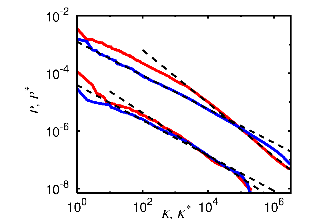
Wikipedia is a useful example of a scale-free network. An article quotes other Wikipedia articles that generates a network of directed links. For Wikipedia of English articles dated by Aug 2009 we have $N=3282257$, $N_{\ell}=71012307$ (Zhirov et al. (2010)). The dependencies of PageRank $P(K)$ and CheiRank $P^{*}(K^{*})$ probabilities on indexes $K$ and $K^{*}$ are shown in Fig. 5. In a large range the decay can be satisfactory described by an algebraic law with an exponent $\beta$. The obtained $\beta$ values are in a reasonable agreement with the expected relation $\beta=1/(\mu_{\rm in,out}-1)$ with the exponents of distribution of links given above. However, the decay is algebraic only on a tail, showing certain nonlinear variations well visible for $P^{*}(K^{*})$ at large values of $P^{*}$.

Similar data for network of University of Cambridge (2006) with $N=212710$, $N_{\ell}=2015265$ Frahm et al. (2011) are shown in the same Fig. 5. Here, the exponents $\beta$ have different values with approximately the same statistical accuracy of $\beta$.

Thus we come to the same conclusion as Meusel et al. (2014): the probability decay of PageRank and CheiRank is only approximately algebraic, the relation between exponents $\beta$ and $\mu$ also works only approximately.

IV.2 Correlator between PageRank and CheiRank

Each network node $i$ has both PageRank $K(i)$ and CheiRank $K(i)^{*}$ indexes so that it is interesting to know what is a correlation between the corresponding vectors of PageRank and CheiRank. It is convenient to characterized this by a correlator introduced in Chepelianskii (2010)

$$\kappa=N\sum^{N}_{i=1}P(K(i))P^{*}(K^{*}(i))-1\;\;.$$ (4)

Figure 6: (Color online) Correlator $\kappa$ as a function of the number of nodes $N$ for different networks: Wikipedia networks, Phys Rev network, 17 UK universities, 10 versions of Kernel Linux Kernel PCN, Escherichia Coli and Yeast Transcription Gene networks, Brain Model Network, C.elegans neural network and Business Process Management Network. After Ermann et al. (2012a) with additional data from Abel and Shepelyansky (2011), Eom and Shepelyansky (2013a), Kandiah and Shepelyansky (2014a), Frahm et al. (2014b).

Figure 7: (Color online) Density distribution of network nodes $W(K,K^{*})=dN_{i}/dKdK^{*}$ shown on the plane of PageRank and CheiRank indexes in logscale $(\log_{N}K,\log_{N}K^{*})$ for all $1\leq K,K^{*}\leq N$, density is computed over equidistant grid in plane $(\log_{N}K,\log_{N}K^{*})$ with $100\times 100$ cells; color shows average value of $W$ in each cell, the normalization condition is $\sum_{K,K^{*}}W(K,K^{*})=1$. Density $W(K,K^{*})$ is shown by color with blue (dark gray) for minimum in (a),(b) and white (a) and yellow (white) (b) for maximum (black for zero). Panel (a): data for Wikipedia Aug (2009), $N=3282257$, green/red (light gray/dark gray) points show top 100 persons from PageRank/CheiRank, yellow (white) pluses show top 100 persons from Hart (1992); after Zhirov et al. (2010). Panel (b): Density distribution $W(K,K^{*})=dN_{i}/dKdK^{*}$ for Linux Kernel V2.4 network with $N=85757$, after Ermann et al. (2012a).

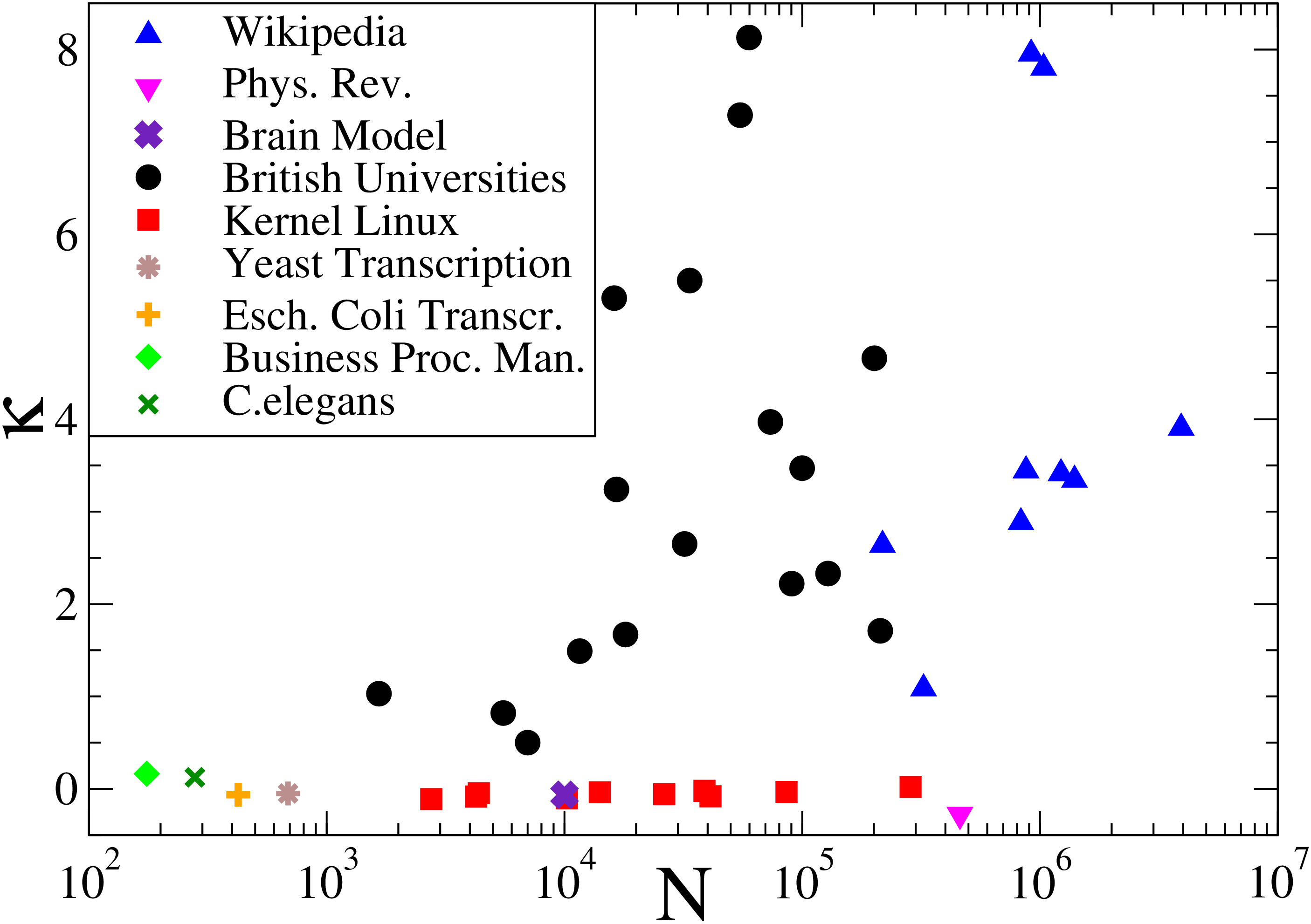
Even if all the networks from Fig. 6 have similar algebraic decay of PageRank probability with $K$ and similar $\beta\sim 1$ exponents we see that the correlations between PageRank and CheiRank vectors are drastically different in these networks. Thus the networks of UK universities and 9 different language editions of Wikipedia have the correlator $\kappa\sim 1-8$ while all other networks have $\kappa\sim 0$. This means that there are significant differences hidden in the network architecture which are no visible from PageRank analysis. We will discuss the possible origins of such a difference for the above networks in next Secs.

IV.3 PageRank-CheiRank plane

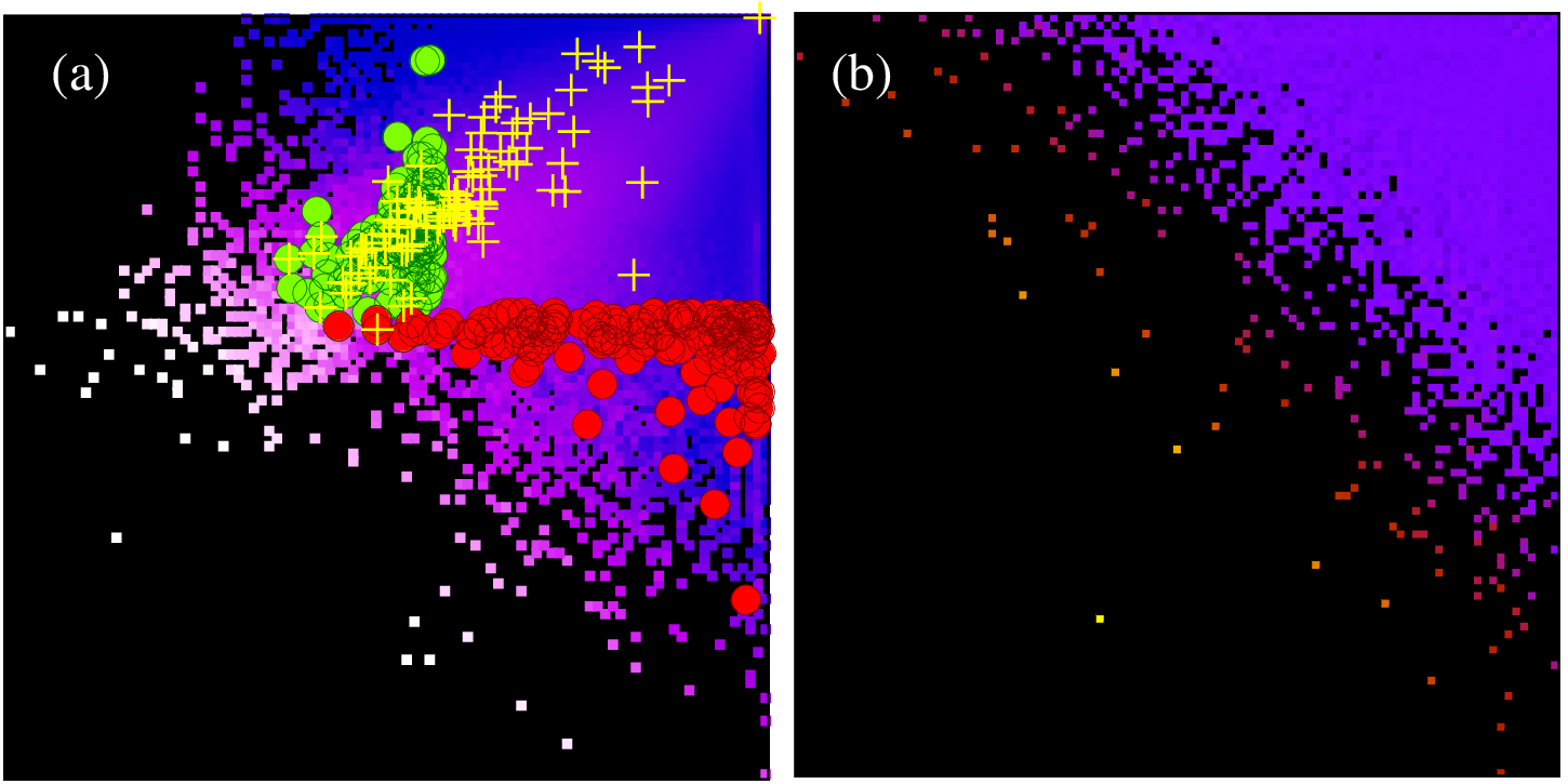
A more detailed characterization of correlations between PageRank and CheiRank vectors can be obtained from a distribution of network nodes on the two-dimensional plane (2D) of indexes $(K,K^{*})$. Two examples for Wikipedia and Linux networks are shown in Fig. 7. A qualitative difference between two networks is obvious. For Wikipedia we have a maximum of density along the line $\ln K^{*}\approx 5+(\ln K)/3$ that results from a strong correlation between PageRank and CheiRank with $\kappa=4.08$. In contrast to that for the Linux network V2.4 we have a homogeneous density distribution of nodes along lines $\ln K^{*}=\ln K+const$ corresponding to uncorrelated probabilities $P(K)$ and $P^{*}(K^{*})$ and even slightly negative value of $\kappa=-0.034$. We note that if for Wikipedia we generate nodes with independent probabilities distributions $P$ and $P^{*}$, obtained from this network at the corresponding value of $N$, then we obtain a homogeneous node distribution in $(K,K^{*})$ plane (in $(\log K,\log K^{*})$ plane it takes a triangular form, see Fig.4 at Zhirov et al. (2010)).

In Fig. 7(a) we also show the distribution of top 100 persons from PageRank and CheiRank compared with the top 100 persons from Hart (1992). There is a significant overlap between PageRank and Hart ranking of persons while CheiRank generates mainly another listing of people. We discuss the Wikipedia ranking of historical figures in Sec. IX.

IV.4 2DRank

PageRank and CheiRank indexes $K_{i}{K_{i}}^{*}$ order all network nodes according to a monotonous decrease of corresponding probabilities $P(K_{i})$ and $P^{*}({K_{i}}^{*})$. While top $K$ nodes are most popular or known in the network, top $K^{*}$ nodes are most communicative nodes with many outgoing links. It is useful to consider an additional ranking $K_{2}$, called 2DRank, which combines properties of both ranks $K$ and $K^{*}$ Zhirov et al. (2010).

The ranking list $K_{2}(i)$ is constructed by increasing $K\rightarrow K+1$ and increasing 2DRank index $K_{2}(i)$ by one if a new entry is present in the list of first $K^{*}<K$ entries of CheiRank, then the one unit step is done in $K^{*}$ and $K_{2}$ is increased by one if the new entry is present in the list of first $K<K^{*}$ entries of CheiRank. More formally, 2DRank $K_{2}(i)$ gives the ordering of the sequence of sites, that   appear inside   the squares   $\left[1,1;\;K=k,K^{\ast}=k;\;\-...\right]$ when one runs progressively from $k=1$ to $N$. In fact, at each step $k\rightarrow k+1$ there are tree possibilities: (i) no new sites on two edges of square, (ii) only one site is on these two edges and it is added in the listing of $K_{2}(i)$ and (iii) two sites are on the edges and both are added in the listing $K_{2}(i)$, first with $K>K^{\ast}$ and second with $K<K^{\ast}$. For (iii) the choice of order of addition in the list $K_{2}(i)$ affects only some pairs of neighboring sites and does not change the main structure of ordering. An illustration example of 2DRank algorithm is given in Fig.7 at Zhirov et al. (2010). For Wikipedia 2DRanking of persons is discussed in Sec. IX.

IV.5 Historical notes on spectral ranking

Starting from the work of Markov Markov (1906) many scientists contributed to the development of spectral ranking of Markov chains. Research of Perron (1907) and Frobenius (1912) led to the Perron-Frobenius theorem for square matrices with positive entries (see e.g. Brin and Stuck (2002)). The detailed historical description of spectral ranking research is reviewed by Franceschet (2011) and Vigna (2013). As described there, the important steps have been done by researchers in psychology, sociology and mathematics including J.R.Seeley (1949), T.-H.Wei (1952), L.Katz (1953), C.H.Hubbell (1965) (see Refs. in the above publications by Franceschet (2011); Vigna (2013)). In the WWW context, the Google matrix in the form (1), with regularization of dangling nodes and damping factor $\alpha$, was introduced by Brin and Page (1998).

A PageRank vector of a Google matrix $G^{*}$ with inverted directions of links has been considered by Fogaras (2003) and Hrisitidis et al. (2008), but no systematic statistical analysis of 2DRanking was presented there. An important step was done by Chepelianskii (2010) who analyzed $\lambda=1$ eigenvectors of $G$ for directed network and of $G^{*}$ for network with inverted links. The comparative analysis of Linux Kernel network and WWW of University of Cambridge demonstrated a significant differences in correlator $\kappa$ values on these networks and different functions of top nodes in $K$ and $K^{*}$. The term CheiRank was coined in Zhirov et al. (2010) to have a clear distinction between eigenvectors of $G$ and $G^{*}$. We note that top PageRank and CheiRank nodes have certain similarities with authorities and hubs appearing in the HITS algorithm Kleinberg (1999). However, the HITS is query dependent while the rank probabilities $P(K_{i})$ and $P^{*}({K_{i}}^{*})$ classify all nodes of the network.

V Complex spectrum and fractal Weyl law

The Weyl law Weyl (1912) gives a fundamental link between the properties of quantum eigenvalues in closed Hamiltonian systems, the Planck constant $\hbar$ and the classical phase space volume. The number of states in this case is determined by the phase volume of a system with dimension $d$. The case of Hermitian operators is now well understood both on mathematical and physical grounds Dimassi and Sjöstrand (1999); Landau and Lifshitz (1989). Surprisingly, only recently it has been realized that the case of nonunitary operators describing open systems in the semiclassical limit has a number of new interesting properties and the concept of the fractal Weyl law Sjöstrand (1990); Zworski (1999) has been introduced to describe the dependence of number of resonant Gamow eigenvalues Gamow (1928) on $\hbar$.

The Gamow eigenstates find important applications for decay of radioactive nuclei, quantum chemistry reactions, chaotic scattering and microlasers with chaotic resonators, open quantum maps (see Gaspard (1998, 2014); Shepelyansky (2008) and Refs. therein). The spectrum of corresponding operators has a complex spectrum $\lambda$. The spread width $\gamma=-2\ln|\lambda|$ of eigenvalues $\lambda$ determines the life time of a corresponding eigenstate. The understanding of the spectral properties of related operators in the semiclassical limit represents an important challenge.

According to the fractal Weyl law Sjöstrand (1990); Lu et al. (2003) the number of Gamow eigenvalues $N_{\gamma}$, which have escape rates $\gamma$ in a finite band width $0\leq\gamma\leq\gamma_{b}$, scales as

$$N_{\gamma}\propto\hbar^{-d/2}\propto N^{d/2}$$ (5)

where $d$ is a fractal dimension of a classical strange repeller formed by classical orbits nonescaping in future and past times. In the context of eigenvalues $\lambda$ of the Google matrix we have $\gamma=-2\ln|\lambda|$. By numerical simulations it has been shown that the law (5) works for a scattering problem in 3-disk system Lu et al. (2003) and quantum chaos maps with absorption when the fractal dimension $d$ is changed in a broad range $0<d<2$ Shepelyansky (2008); Ermann and Shepelyansky (2010b).

The fractal Weyl law (5) of open systems with a fractal dimension $d<2$ leads to a striking consequence: only a relatively small fraction of eigenvalues $\mu_{W}\sim N_{\gamma}/N\propto\hbar^{(2-d)/2}\propto N^{(d-2)/2}\ll 1$ has finite values of $|\lambda|$ while almost all eigenstates of the matrix operator of size $N\propto 1/\hbar$ have $\lambda\rightarrow 0$. The eigenstates with finite $|\lambda|>0$ are related to the classical fractal sets of orbits non-escaping neither in the future neither in the past. A fractal structure of these quantum fractal eigenstates has been investigated in Shepelyansky (2008). There it was conjectured that the eigenstates of a Google matrix with finite $|\lambda|>0$ will select interesting specific communities of a network. We will see below that the fractal Weyl law can indeed be observed in certain directed networks and in particular we show in the next section that it naturally appears for Perron-Frobenius operators of dynamical systems and Ulam networks.

It is interesting to note that nontrivial complex spectra also naturally appear in systems of quantum chaos in presence of a contact with a measurement device Bruzda et al. (2010). The properties of complex spectra of small size orthostochastic (unistochastic) matrices are analyzed in Zyczkowski et al. (2003). In such matrices the elements can be presented in a form $S_{ij}=O^{2}_{ij}$ ($S_{ij}=|U_{ij}|^{2}$) where $O$ is an orthogonal matrix ( $U$ is a unitary matrix). We will see certain similarities of their spectra with the spectra of directed networks discussed in Sec. VIII.

Recent mathematical results for the fractal Weyl law are presented in Nonnenmacher and Zworski (2007); Nonnenmacher et al. (2014).

Figure 8: Illustration of operation of the Ulam method: the phase space $(x,y)$ is divided in $N=N_{x}\times N_{y}$ cells, $N_{c}$ trajectories start from cell $j$ and the number of trajectories $N_{ij}$ arrived to a cell $i$ from a cell $j$ is collected after a map iteration. Then the matrix of Markov transitions is defined as $S_{ij}=N_{ij}/N_{c}$, by construction $\sum_{i=1}^{N}S_{ij}=1$.

VI Ulam networks

By construction the Google matrix belongs to the class of Perron-Frobenius operators which naturally appear in ergodic theory Cornfeldet al. (1982) and dynamical systems with Hamiltonian or dissipative dynamics Brin and Stuck (2002). In 1960 Ulam Ulam (1960) proposed a method, now known as the Ulam method, for a construction of finite size approximants for the Perron-Frobenius operators of dynamical maps. The method is based on discretization of the phase space and construction of a Markov chain based on probability transitions between such discrete cells given by the dynamics. Using as an example a simple chaotic map Ulam made a conjecture that the finite size approximation converges to the continuous limit when the cell size goes to zero. Indeed, it has been proven that for hyperbolic maps in one and higher dimensions the Ulam method converges to the spectrum of continuous system Li (1976); Blank et al. (2002). The probability flows in dynamical systems have rich and nontrivial features of general importance, like simple and strange attractors with localized and delocalized dynamics governed by simple dynamical rules Lichtenberg and Lieberman (1992). Such objects are generic for nonlinear dissipative dynamics and hence can have relevance for actual WWW structure. The analysis of Ulam networks, generated by the Ulam method, allows to obtain a better intuition about the spectral properties of Google matrix. The term Ulam networks was introduced in Shepelyansky and Zhirov (2010a).

VI.1 Ulam method for dynamical maps

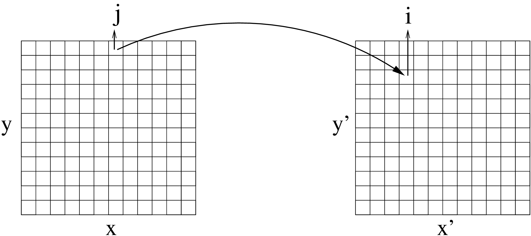
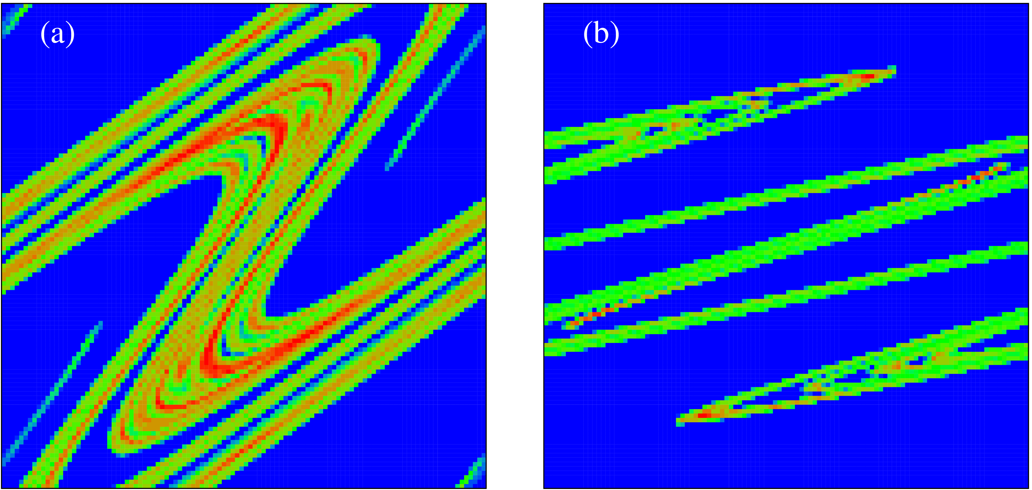
In Fig. 8 we show how the Ulam method works. The phase space of a dynamical map is divided in equal cells and a number of trajectories $N_{c}$ is propagated by a map iteration. Thus a number of trajectories $N_{ij}$ arrived from cell $j$ to cell $i$ is determined. Then the matrix of Markov transition is defined as $S_{ij}=N_{ij}/N_{c}$. By construction this matrix belongs to the class of Perron-Frobenius operators which includes the Google matrix.

The physical meaning of the coarse grain description by a finite number of cells is that it introduces in the system a noise of cell size amplitude. Due to that an exact time reversibility of dynamical equations of chaotic maps is destroyed due to exponential instability of chaotic dynamics. This time reversibility breaking is illustrated by an example of the Arnold cat map by Ermann and Shepelyansky (2012b). For the Arnold cat map on a long torus it is shown that the spectrum of the Ulam approximate of the Perron-Frobenius (UPFO) is composed of a large group of complex eigenvalues with $\gamma\sim 2h\approx 2$, and real eigenvalues with $|1-\lambda|\ll 1$ corresponding to a statistical relaxation to the ergodic state at $\lambda=1$ described by the Fokker-Planck equation (here $h$ is the Kolmogorov-Sinai entropy of the map being here equal to the Lyapunov exponent, see e.g. Chirikov (1979)).

For fully chaotic maps the finite cell size, corresponding to added noise, does not significantly affect the dynamics and the discrete UPFO converges to the limiting case of continuous Perron-Frobenius operator Li (1976); Blank et al. (2002). The Ulam method finds useful applications in studies of dynamics of molecular systems and coherent structures in dynamical flows Froyland and Padberg (2009). Additional Refs. can be found in Frahm and Shepelyansky (2010).

VI.2 Chirikov standard map

However, for symplectic maps with a divided phase space, a noise present in the Ulam method significantly affects the original dynamics leading to a destruction of islands of stable motion and Kolmogorov-Arnold-Moser (KAM) curves. A famous example of such a map is the Chirikov standard map which describes the dynamics of many physical systems Chirikov (1979); Chirikov and Shepelyansky (2008):

$${\bar{y}}=\eta y+\frac{K_{s}}{2\pi}\sin(2\pi x)\;,\;\;{\bar{x}}=x+{\bar{y}}\;\;({\rm mod}\;1)\;.$$ (6)

Here bars mark the variables after one map iteration and we consider the dynamics to be periodic on a torus so that $0\leq x\leq 1$, $-1/2\leq y\leq 1/2$; $K_{s}$ is a dimensionless parameter of chaos. At $\eta=1$ we have area-preserving symplectic map, considered in this SubSec., for $0<\eta<1$ we have a dissipative dynamics analyzed in next SubSec.

Figure 9: (Color online) Complex spectrum of eigenvalues $\lambda_{j}$, shown by red/gray dots, for the UPFO of two variants of the Chirikov standard map (6); the unit circle $|\lambda|=1$ is shown by a green (light gray) curve, the unit eigenvalue at $\lambda=1$ is shown as larger red/gray dot. Panel (a) corresponds to the Chirikov standard map at dissipation $\eta=0.3$ and $K_{s}=7$; the phase space is covered by $110\times 110$ cells and the UPFO is constructed by many trajectories with random initial conditions generating transitions from one cell into another (after Ermann and Shepelyansky (2010b)). Panel (b) corresponds to the Chirikov standard map without dissipation at $K_{s}=0.971635406$ with an UPFO constructed from a single trajectory of length $10^{12}$ in the chaotic domain and $280\times 280/2$ cells to cover the phase space (after Frahm and Shepelyansky (2010)).

Figure 10: (Color online) Density plots of absolute values of the eigenvectors of the UPFO obtained by the generalized Ulam method with a single trajectory of $10^{12}$ iterations of the Chirikov standard map at $K_{s}=0.971635406$. The phase space is shown in the area $0\leq x\leq 1$, $0\leq y\leq 1/2$; the UPFO is obtained from $M\times M/2$ cells placed in this area. Panels represent: (a) eigenvector $\psi_{0}$ with eigenvalue $\lambda_{0}=1$; (b) eigenvector $\psi_{2}$ with real eigenvalue $\lambda_{2}=0.99878108$; (c) eigenvector $\psi_{6}$ with complex eigenvalue $\lambda_{6}=-0.49699831+i\,0.86089756\approx|\lambda_{6}|\,e^{i\,2\pi/3}$; (d) eigenvector $\psi_{13}$ with complex eigenvalue $\lambda_{13}=0.30580631+i\,0.94120900\approx|\lambda_{13}|\,e^{i\,2\pi/5}$. Panel (a) corresponds to $M=25$ while (b), (c) and (d) have $M=800$. Color is proportional to amplitude with blue (black) for zero and red (gray) for maximal value. After Frahm and Shepelyansky (2010).

Since the finite cell size generates noise and destroys the KAM curves in the map (6) at $\eta=1$, one should use the generalized Ulam method Frahm and Shepelyansky (2010), where the transition probabilities $N_{ij}/N_{c}$ are collected along one chaotic trajectory. In this construction a trajectory visits only those cells which belong to one connected chaotic component. Therefore the noise induced by the discretization of the phase space does not lead to a destruction of invariant curves, in contrast to the original Ulam method Ulam (1960), which uses all cells in the available phase space. Since a trajectory is generated by a continuous map it cannot penetrate inside the stability islands and on a physical level of rigor one can expect that, due to ergodicity of dynamics on one connected chaotic component, the UPFO constructed in such a way should converge to the Perron-Frobenius operator of the continuous map on a given subspace of chaotic component. The numerical confirmations of this convergence are presented in Frahm and Shepelyansky (2010).

We consider the map (6) at $K_{s}=0.971635406$ when the golden KAM curve is critical. Due to the symmetry of the map with respect to $x\to 1-x$ and $y\to-y$ we can use only the upper part of the phase space with $y\geq 0$ dividing it in $M\times M/2$ cells. At that $K_{s}$ we find that the number of cells visited by the trajectory in this half square scales as $N_{d}\approx C_{d}M^{2}/2$ with $C_{d}\approx 0.42$. This means that the chaotic component contains about $40\%$ of the total area which is in good agreement with the known result of Chirikov (1979).

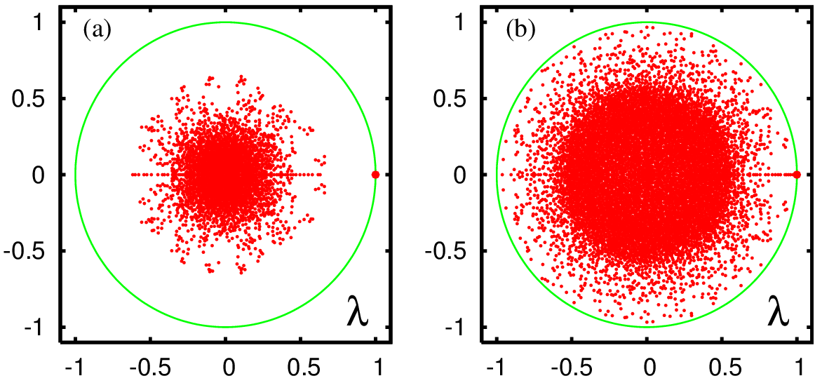
The spectrum of the UPFO matrix $S$ for the phase space division by $280\times 208/2$ cells is shown in Fig. 9(b). In a first approximation the spectrum $\lambda$ of $S$ is more or less homogeneously distributed in the polar angle $\varphi$ defined as $\lambda_{j}=|\lambda_{j}|\exp(i\varphi_{j})$. With the increase of matrix size $N_{d}$ the two-dimensional density of states $\rho(\lambda)$ converges to a limiting distribution Frahm and Shepelyansky (2010). With the help of the Arnoldi method it is possible to compute a few thousands of eigenvalues with largest absolute values $|\lambda|$ for maximal $M=1600$ with the total matrix size $N=N_{d}\approx 5.3\times 10^{5}$.

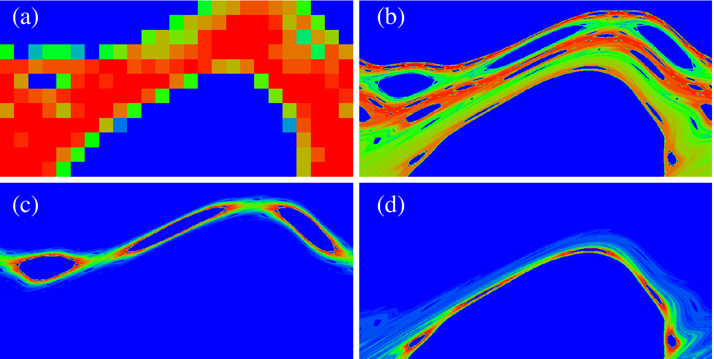
The eigenstate at $\lambda=1$ is homogeneously distributed over the chaotic component at $M=25$ (Fig. 10) and higher $M$ values Frahm and Shepelyansky (2010). This results from the ergodicity of motion and the fact that for symplectic maps the measure is proportional to the phase space area Chirikov (1979); Cornfeldet al. (1982). Examples of other right eigenvalues of $S$ at real and complex eigenvalues $\lambda$ with $|\lambda|<1$ are also shown in Fig. 10. For $\lambda_{2}$ the eigenstate corresponds to some diffusive mode with two nodal lines, while other two eigenstates are localized around certain resonant structures in phase space. This shows that eigenstates of the matrix $G$ (and $S$) are related to specific communities of a network.

With the increase of number of cells $M^{2}/2$ there are eigenvalues which become more and more close to the unit eigenvalue. This is shown to be related to an algebraic statistics of Poincaré recurrences and long time sticking of trajectories in a vicinity of critical KAM curves. At the same time for symplectic maps the measure is proportional to area so that we have dimension $d=2$ and hence we have a usual Weyl law with $N_{\gamma}\propto N$. More details can be found at Frahm and Shepelyansky (2010, 2013).

Figure 11: (Color online) Phase space representation of eigenstates of the UFPO $S$ for $N=110\times 110$ cells (color is proportional to absolute value $|\psi_{i}|$ with red/gray for maximum and blue/black for zero). Panel (a) shows an eigenstate with maximum eigenvalue $\lambda_{1}=0.756$ of the UFPO of map (6) with absorption at $K_{s}=7$, $a=2$, $\eta=1$, the space region is ($-aK_{s}/4\pi\leq y\leq aK_{s}/4\pi$, $0\leq x\leq 1$), the fractal dimension of the strange repeller set nonescaping in future is $d_{e}=1+d/2=1.769$. Panel (b) shows an eigenstate at $\lambda=1$ of the UFPO of map (6) without absorption at $K_{s}=7$, $\eta=0.3$, the shown space region is ($-1/\pi\leq y\leq 1/\pi$, $0\leq x\leq 1$) and the fractal dimension of the strange attractor is $d=1.532$. After Ermann and Shepelyansky (2010b).

VI.3 Dynamical maps with strange attractors

The fractal Weyl law (5) has initially been proposed for quantum systems with chaotic scattering. However, it is natural to assume that it should also work for Perron-Frobenius operators of dynamical systems. Indeed, the mathematical results for the Selberg zeta function indicated that the law (5) should remain valid for the UFPO (see Refs. at Nonnenmacher et al. (2014)). A detailed test of this conjecture Ermann and Shepelyansky (2010b) has been performed for the map (6) with dissipation at $0<\eta<1$, when at large $K_{s}$ the dynamics converges to a strange attractor in the range $-2<y<2$, and for the nondissipative case $\eta=1$ with absorption where all orbits leaving the interval $-aK_{s}/4\pi\leq y\leq aK_{s}/4\pi$ are absorbed after one iteration (in both cases there is no modulus in $y$).

An example of the spectrum of UPFO for the model with dissipation is shown in Fig. 9(a). We see that now, in contrast to the symplectic case of Fig. 9(b), the spectrum has a significant gap which separates the eigenvalue $\lambda=1$ from the other eigenvalues with $|\lambda|<0.7$. For the case with absorption the spectrum has a similar structure but now with $|\lambda|<1$ for the leading eigenvalue $\lambda$ since the total number of initial trajectories decreases with the number of map iterations due to absorption implying that for this case $\sum_{i}S_{ij}<1$ with $S$ being the UPFO.

It is established that the distribution of density of states $dW/d\gamma$ (or $dW/d|\lambda|$) converges to a fixed distribution in the limit of large $N$ or cell size going to zero Ermann and Shepelyansky (2010b) (see Fig.4 there). This demonstrates the validity of the Ulam conjecture for considered systems.

Examples of two eigenstates of the UFPO for these two models are shown in Fig. 11. The fractal structure of eigenstates is well visible. For the dissipative case without absorption we have eigenstates localized on the strange attractor. For the case with absorption eigenstates are located on a strange repeller corresponding to an invariant set of nonescaping orbits. The fractal dimension $d$ of these classical invariant sets can be computed by the usual box-counting method for dynamical systems. It is important to note that for the case with absorption it is more natural to measure the dimension $d_{e}$ of the set of orbits nonescaping in future. Due to the time reversal symmetry of the continuous map the dimension of the set of orbits nonescaping in the past is also $d_{e}$. Thus the phase space dimension $2$ is composed of $2=d_{e}+d_{e}-d$ and $d_{e}=1+d/2$ where $d$ is the dimension of the invariant set of orbits nonescaping neither in the future neither in the past. For the case with dissipation without absorption all orbits drop on a strange attractor and we have the dimension of invariant set $d_{e}=d$.

VI.4 Fractal Weyl law for Perron-Frobenius operators

Figure 12: (Color online) Panel (a) shows the dependence of the integrated number of states $N_{\gamma}$ with decay rates $0\leq\gamma\leq\gamma_{b}=16$ on the size $N$ of the UFPO matrix $S$ for the map (6) at $K_{s}=7$. The fits of numerical data, shown by dashed straight lines, give $\nu=0.590,d_{e}=1+d/2=1.643$ (at $a=1$); $\nu=0.772,d_{e}=1+d/2=1.769$ (at $a=2$); $\nu=0.716,d=1.532$ (at $\eta=0.3$); $\nu=0.827,d=1.723$ (at $\eta=0.6$). Panel (b) shows the fractal Weyl exponent $\nu$ as a function of fractal dimension $d$ of the invariant fractal set for the map (6) with a strange attractor $(\eta<1)$ at $K_{s}=15$ (green/gray crosses), $K_{s}=12$ (red/gray squares), $K_{s}=10$ (orange/gray stars), $K_{s}=7$ blue/black triangles; for a strange repeller $(\eta=1)$ at $K_{s}=7$ (black points) and for a strange attractor for the Hénon map at standard parameters $a=1.2;1.4$, $b=0.3$ (green diamonds). The straight dashed line shows the fractal Weyl law dependence $\nu=d/2$. After Ermann and Shepelyansky (2010b).

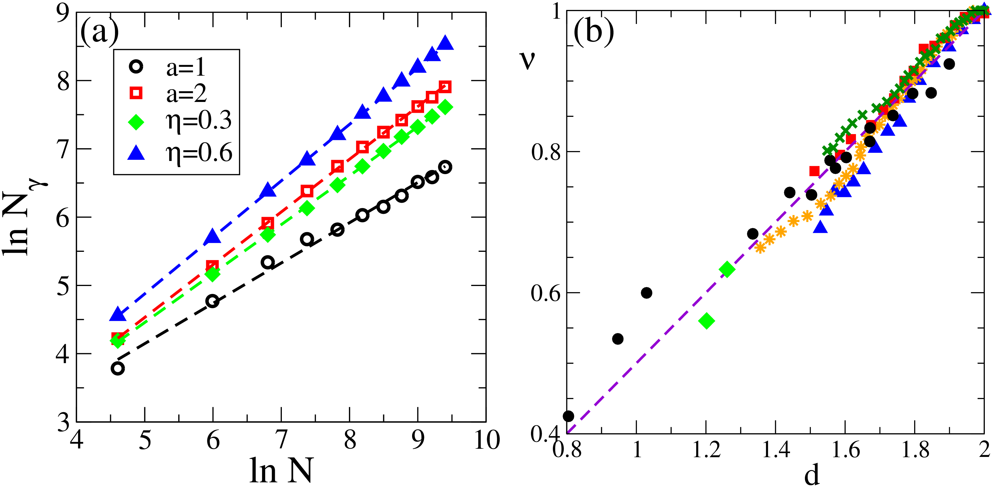
The direct verification of the validity of the fractal Weyl law (5) is presented in Fig. 12. The number of eigenvalues $N_{\gamma}$ in a range with $0\leq\gamma\leq\gamma_{b}$ ($\gamma=-2\ln|\lambda|$) is numerically computed as a function of matrix size $N$. The fit of the dependence $N_{\gamma}(N)$, as shown in Fig. 12(a), allows to determine the exponent $\nu$ in the relation $N_{\gamma}\propto N^{\nu}$. The dependence of $\nu$ on the fractal dimension $d$, computed from the invariant fractal set by the box-counted method, is shown in Fig. 12(b). The numerical data are in good agreement with the theoretical fractal Weyl law dependence $\nu=d/2$. This law works for a variety of parameters for the system (6) with absorption and dissipation, and also for a strange attractor in the Hénon map (${\bar{x}}=y+1-ax^{2},{\bar{y}}=bx$). We attribute certain deviations, visible in Fig. 12 especially for $K_{s}=7$, to the fact that at $K_{s}=7$ there is a small island of stability at $\eta=1$, which can produce certain influence on the dynamics.

The physical origin of the law (5) can be understood in a simple way: the number of states $N_{\gamma}$ with finite values of $\gamma$ is proportional to the number of cells $N_{f}\propto N^{d/2}$ on the fractal set of strange attractor. Indeed, the results for the overlap measure show that the eigenstates $N_{\gamma}$ have a strong overlap with the steady state while the states with $\lambda\rightarrow 0$ have very small overlap. Thus almost all $N$ states have eigenvalues $\lambda\rightarrow 0$ and only a small fraction of states on a strange attractor/repeller $N_{\gamma}\propto N_{f}\propto N^{d/2}\ll N$ has finite values of $\lambda$. We also checked that the participation ratio $\xi$ of the eigenstate at $\lambda=1$, grows as $\xi\sim N_{f}\propto N^{d/2}$ in agreement with the fractal Weyl law Ermann and Shepelyansky (2010b).

VI.5 Intermittency maps

The properties of the Google matrix generated by one-dimensional intermittency maps are analyzed in Ermann and Shepelyansky (2010a). It is found that for such Ulam networks there are many eigenstates with eigenvalues $|\lambda|$ being very close to unity. The PageRank of such networks at $\alpha=1$ is characterized by a power law decay with an exponent determined by the parameters of the map. It is interesting to note that usually for WWW the PageRank probability is proportional to a number of ingoing links distribution (see e.g. Litvak et al. (2008)). For the case of intermittency maps the decay of PageRank is independent of number of ingoing links. In addition, for $\alpha$ close to unity a decay of the PageRank has an exponent $\beta\approx 1$ but at smaller values $\alpha\leq 0.9$ the PageRank becomes completely delocalized. It is shown that the delocalization depends on the intermittency exponent of the map. This indicates that a rather dangerous phenomenon of PageRank delocalization can appear for certain directed networks. At the same time the one-dimensional intermittency map still generates a relatively simple structure of links with a typical number of links per node being close to unity. Such a case is probably not very typical for real networks. Therefore it is useful to analyze richer Ulam networks with a larger number of links per node.

VI.6 Chirikov typical map

With this aim we consider the Ulam networks generated by the Chirikov typical map with dissipation studied by Shepelyansky and Zhirov (2010a). The map introduced, by Chirikov in 1969 for description of continuous chaotic flows, has the form:

$$y_{t+1}=\eta y_{t}+k_{s}\sin(x_{t}+\theta_{t})\;,\;\;x_{t+1}=x_{t}+y_{t+1}\;.$$ (7)

Here the dynamical variables $x,y$ are taken at integer moments of time $t$. Also $x$ has a meaning of phase variable and $y$ is a conjugated momentum or action. The phases $\theta_{t}=\theta_{t+T}$ are $T$ random phases periodically repeated along time $t$. We stress that their $T$ values are chosen and fixed once and they are not changed during the dynamical evolution of $x,y$. We consider the map in the region of Fig. 13 ($0\leq x<2\pi,-\pi\leq y<\pi$) with the $2\pi$-periodic boundary conditions. The parameter $0<\eta<1$ gives a global dissipation. The properties of the symplectic map at $\eta=1$ have been studied in detail in Frahm and Shepelyansky (2009). The dynamics is globally chaotic for $k_{s}>k_{c}\approx 2.5/T^{3/2}$ and the Kolmogorov-Sinai entropy is $h\approx 0.29{k_{s}}^{2/3}$ (more details about the Kolmogorov-Sinai entropy can be found in Brin and Stuck (2002); Chirikov (1979); Cornfeldet al. (1982)). A bifurcation diagram at $\eta<1$ shows a series of transitions between fixed points, simple and strange attractors. Here we present results for $T=10$, $k_{s}=0.22$, $\eta=0.99$ and a specific random set of $\theta_{t}$ given in Shepelyansky and Zhirov (2010a).

Figure 13: (Color online) PageRank probability $P_{j}$ for the Google matrix generated by the Chirikov typical map at $T=10$, $k_{s}=0.22$, $\eta=0.99$ with $\alpha=1$ (a), $\alpha=0.95$ (b), and $\alpha=0.85$ (c). The probability $P_{j}$ is shown in the phase space region $0\leq x<2\pi;-\pi\leq y<\pi$ which is divided in $N=3.6\cdot 10^{5}$ cells; $P_{j}$ is zero for blue/black and maximal for red/gray. After Shepelyansky and Zhirov (2010a).

Due to exponential instability of motion one cell in the Ulam method gives transitions approximately to $k_{\rm cl}\approx\exp(hT)$ other cells. According to this relation a large number of cells $k_{\rm cl}$ can be coupled at large $T$ and $h$. For parameters of Fig. 13 one finds an approximate power law distribution of ingoing and outgoing links in the corresponding Ulam network with the exponents $\mu_{\rm in}\approx\mu_{\rm out}\approx 1.9$. The variation of the PageRank vector with the damping factor $\alpha$ is shown in Fig. 13 on the phase plane $(x,y)$. For $\alpha=1$ the PageRank is concentrated in a vicinity of a simple attractor composed of several fixed points on the phase plane. Thus the dynamical attractors are the most popular nodes from the network view point. With a decrease of $\alpha$ down to $0.95,0.85$ values we find a stronger and stronger delocalization of PageRank over the whole phase space.

The delocalization with a decrease of $\alpha$ is also well seen in Fig. 14 where we show $P_{j}$ dependence on PageRank index $j$ with a monotonic decreasing probability $P_{j}$. At $\alpha=1$ we have an exponential decay of $P_{j}$ with $j$ that corresponds to a Boltzmann type distribution where a noise produced by a finite cell size in the Ulam method is compensated by dissipation. For $\alpha=0.95$ the random jumps of a network surfer, induced by the term $(1-\alpha)/N$ in (1), produce an approximate power law decay of $P_{j}\propto 1/j^{\beta}$ with $\beta\approx 0.48$. For $\alpha=0.85$ the PageRank probability is flat and completely delocalized over the whole phase space.

Figure 14: (Color online) Dependence of PageRank probability $P_{j}$ on PageRank index $j$ for number of cells in the UFPO being $N=10^{4}$, $9\times 10^{4}$, $3.6\times 10^{5}$ and $1.44\times 10^{6}$ (larger $N$ have more dark and more long curves in (b), (c); in (a) this order of $N$ is for curves from bottom to top (curves for $N=3.6\times 10^{5}$ and $1.44\times 10^{6}$ practically coincide in this panel; for online version we note that the above order of $N$ values corresponds to red, magenta, green, blue curves respectively). Dashed line in (a) shows an exponential Boltzmann decay (see text, line is shifted in $j$ for clarity). The dashed straight line in (b) shows the fit $P_{j}\sim 1/j^{\beta}$ with $\beta=0.48$. Other parameters, including the values of $\alpha$, and panel order are as in Fig. 13. After Shepelyansky and Zhirov (2010a).

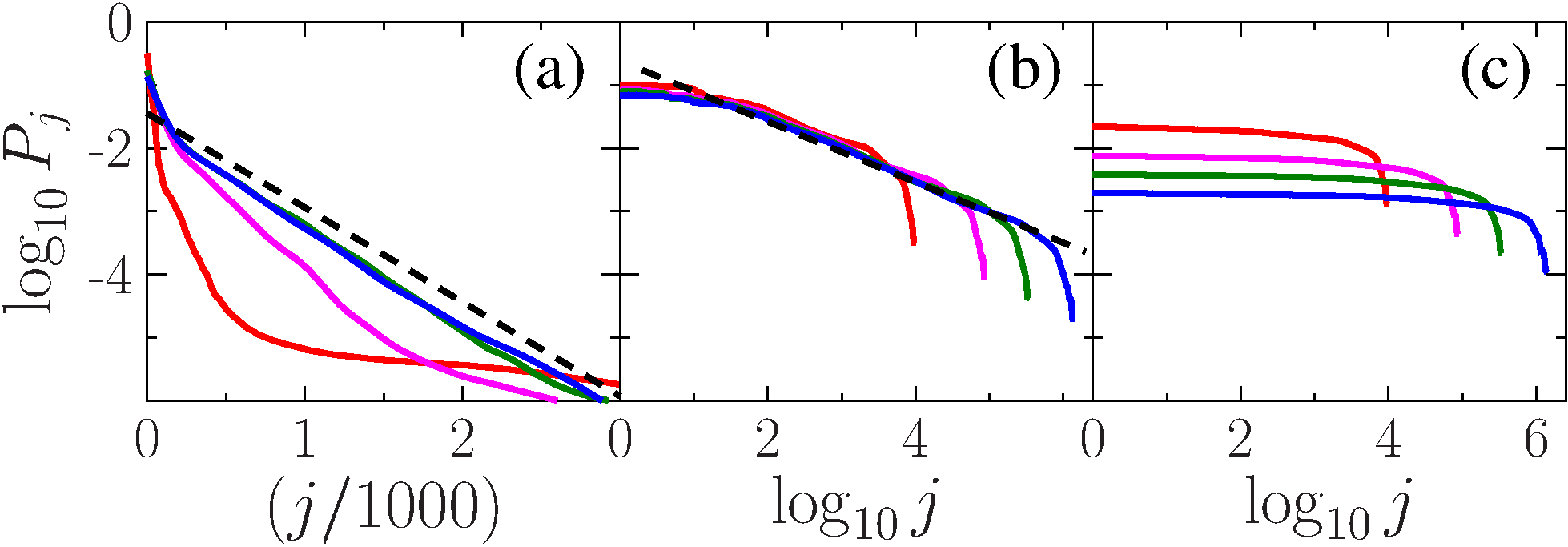
The analysis of the spectrum of $S$ for the map (7) for the parameters of Fig. 14 shows the existence of eigenvalues being very close to $\lambda=1$, however, there is no exact degeneracy as it is the case for UK universities which we will discuss below. The spectrum is characterized by the fractal Weyl law with the exponent $\nu\approx 0.85$. For eigenstates with $|\lambda|<1$ the values of IPR $\xi$ are less than $300$ for a matrix size $N\approx 1.4\times 10^{4}$ showing that eigenstates are localized. However, for the PageRank the computations can be done with larger matrix sizes reaching a maximal value of $N=6.4\times 10^{5}$. The dependence of $\xi$ on $\alpha$ shows that a delocalization transition of PageRank vector takes place for $\alpha<\alpha_{c}\approx 0.95$. Indeed, at $\alpha=0.98$ we have $\xi\approx 30$ while at $\alpha\approx 0.8$ the IPR value of PageRank becomes comparable with the whole system size $\xi\approx 5\times 10^{5}\sim N=6.4\times 10^{5}$ (see Fig.9 at Shepelyansky and Zhirov (2010a)).

The example of Ulam networks considered here shows that a dangerous phenomenon of PageRank delocalization can take place under certain conditions. This delocalization may represent a serious danger for efficiency of search engines since for a delocalized flat PageRank the ranking of nodes becomes very sensitive to small perturbations and fluctuations.

VII Linux Kernel networks

Modern software codes represent now complex large scale structures and analysis and optimization of their architecture become a challenge. An interesting approach to this problem, based on a directed network construction, has been proposed by Chepelianskii (2010). Here we present results obtained for such networks.

VII.1 Ranking of software architecture

Following Chepelianskii (2010) we consider the Procedure Call Networks (PCN) for open source programs with emphasis on the code of Linux Kernel Linux (2010) written in the C programming language Kernighan and Ritchie (1978). In this language the code is structured as a sequence of procedures calling each other. Due to that feature the organization of a code can be naturally represented as a PCN, where each node represents a procedure and each directed link corresponds to a procedure call. For the Linux source code such a directed network is built by its lexical scanning with the identification of all the defined procedures. For each of them a list keeps track of the procedures calls inside their definition.

An example of the obtained network for a toy code with two procedures start_kernel and printk is shown in Fig. 15. The in/out-degrees of this model, noted as $k$ and ${\bar{k}}$, are shown in Fig. 15. These numbers correspond to the number of out/in-going calls for each procedure. The obtained in/out-degree probability distributions $P_{\rm\,in}(k)$, $P_{\rm\,out}({\bar{k}})$ are shown Fig. 15 for different Linux Kernel releases. These distributions are well described by power law dependencies $P_{\rm\,in}(k)\propto 1/k^{\mu_{\rm in}}$ and $P_{\rm\,out}({\bar{k}})\propto 1/{\bar{k}}^{\mu_{\rm out}}$ with $\mu_{\rm in}=2.0\pm 0.02$, and $\mu_{\rm out}=3.0\pm 0.1$. These values of exponents are close to those found for the WWW Donato et al. (2004); Pandurangan et al. (2005). If only calls to distinct functions are counted in the outdegree distribution then the exponent drops to $\mu_{\rm out}\approx 5$ whereas $\mu_{\rm in}$ remains unchanged. It is important that the distributions for the different kernel releases remain stable even if the network size increases from $N=2751$ for version V1.0 to $N=285509$ for the latest version V2.6.32 taken into account in this study. This confirms the free-scale structure of software architecture of Linux Kernel network.

The probability distributions of PageRank and CheiRank vectors are also well described by power laws with exponents $\beta_{\rm in}\approx 1$ and $\beta_{\rm out}\approx 0.5$ being in good agreement with the usual relation $\beta=1/(\mu-1)$ (see Fig.2 in Chepelianskii (2010)). For V2.6.32 the top three procedures of PageRank at $\alpha=0.85$ are printk, memset, kfree with probabilities $0.024,0.012,0.011$ respectively, while at the top of CheiRank we have start_kernel, btrfs_ioctl, menu_finalize with respectively $0.000280,0.000255,0.000250$. These procedures perform rather different tasks with printk reporting messages and start_kernel initializing the Kernel and managing the repartition of tasks. This gives an idea that both PageRank and CheiRank order can be useful to highlight en different aspects of directed and inverted flows on our network. Of course, in the context of WWW ingoing links related to PageRank are less vulnerable as compared to outgoing links related to CheiRank, which can be modified by a user rather easily. However, in other type of networks both directions of links appear in a natural manner and thus both vectors of PageRank and CheiRank play an important and useful role.

Figure 15: (Color online) The diagram in the center represents the PCN of a toy kernel with two procedures written in C-programming language. The data on panels (a) and (b) show outdegree and indegree probability distributions $P_{\rm\,out}({\bar{k}})$ and $P_{\rm\,in}(k)$ respectively. The colors correspond to different Kernel releases. The most recent version 2.6.32, with $N=285509$ and an average $3.18$ calls per procedure, is represented in red/gray. Older versions (2.4.37.6, 2.2.26, 2.0.40, 1.2.12, 1.0) with $N$ respectively equal to (85756, 38766, 14079, 4358, 2751) follow the same behavior. The dashed curve in (a) shows the outdegree probability distribution if only calls to distinct destination procedures are kept. After Chepelianskii (2010).

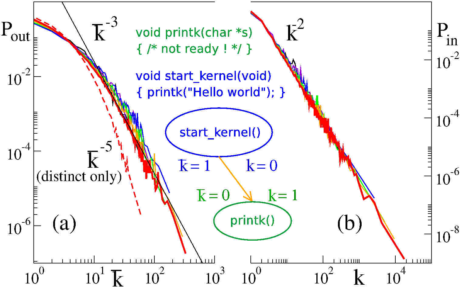
For the Linux Kernel network the correlator $\kappa$ (4) between PageRank and CheiRank vectors is close to zero (see Fig. 6). This confirms the independence of two vectors. The density distribution of nodes of the Linux Kernel network, shown in Fig. 7(b), has a homogeneous distribution along $\ln K+\ln K^{*}=const$ lines demonstrating once more absence of correlations between $P(K_{i})$ and $P^{*}({K_{i}}^{*})$. Indeed, such homogeneous distributions appear if nodes are generated randomly with factorized probabilities $P_{i}{P_{i}}^{*}$ Chepelianskii (2010); Zhirov et al. (2010). Such a situation seems to be rather generic for software architecture. Indeed, other open software codes also have a small values of correlator, e.g. OpenSource software including Gimp 2.6.8 has $\kappa=-0.068$ at $N=17540$ and X Windows server R7.1-1.1.0 has $\kappa=-0.027$ at $N=14887$. In contrast to these software codes the Wikipedia networks have large values of $\kappa$ and inhomogeneous distributions in $(K,K^{*})$ plane (see Figs. 6,7).

The physical reasons for absence of correlations between $P(K)$ and $P^{*}(K^{*})$ have been explained in Chepelianskii (2010) on the basis of the concept of “separation of concerns” in software architecture Dijkstra (1982). It is argued that a good code should decrease the number of procedures that have high values of both PageRank and CheiRank since such procedures will play a critical role in error propagation since they are both popular and highly communicative at the same time. For example in the Linux Kernel, do_fork, that creates new processes, belongs to this class. Such critical procedures may introduce subtle errors because they entangle otherwise independent segments of code. The above observations suggest that the independence between popular procedures, which have high $P(K_{i})$ and fulfill important but well defined tasks, and communicative procedures, which have high $P^{*}({K_{i}}^{*})$ and organize and assign tasks in the code, is an important ingredient of well structured software.

VII.2 Fractal dimension of Linux Kernel Networks

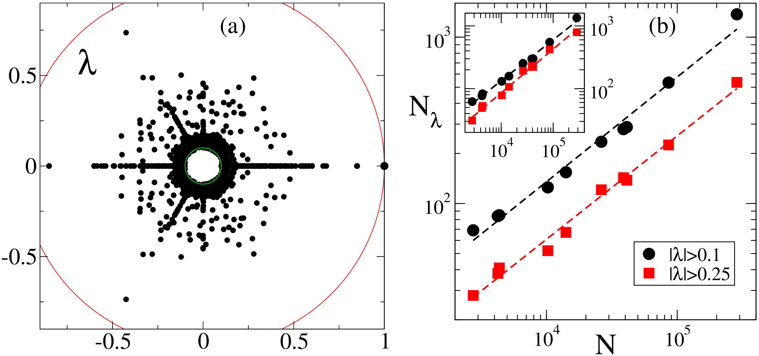
The spectral properties the Linux Kernel network are analyzed in Ermann et al. (2011a). At large $N$ the spectrum is obtained with the help of Arnoldi method from ARPACK library. This allows to find eigenvalues with $|\lambda|>0.1$ for the maximal $N$ at V2.6.32. An example of complex spectrum $\lambda$ of $G$ is shown in Fig. 16(a). There are clearly visible lines at real axis and polar angles $\varphi=\pi/2,2\pi/3,4\pi/3,3\pi/2$. The later are related to certain cycles in procedure calls, e.g. an eigenstate at $\lambda_{i}=0.85\exp(i2\pi/3)$ is located only on 6 nodes. The spectrum of $G^{*}$ has a similar structure.

The network size $N$ grows with the version number of Linux Kernel corresponding to its evolution in time. We determine the total number of states $N_{\lambda}$ with $0.1<|\lambda|\leq 1$ and $0.25<|\lambda|\leq 1$. The dependence of $N_{\lambda}$ on $N$, shown in Fig. 16(b), clearly demonstrates the validity of the fractal Weyl law with the exponent $\nu\approx 0.63$ for $G$ (we find $\nu^{*}\approx 0.65$ for $G^{*}$). We take the values of $\nu$ for $\lambda=0.1$ where the number of eigenvalues $N_{\lambda}$ gives a better statistics. Within statistical errors the value of $\nu$ is not sensitive to the cutoff value at small $\lambda$. The matrix $G^{*}$ has slightly higher values of $\nu$. These results show that the PCN of Linux Kernel has a fractal dimension $d=2\nu\approx 1.26$ for $G$ and $d=2\nu\approx 1.3$ for $G^{*}$.

Figure 16: (Color online) Panel (a) shows distribution of eigenvalues $\lambda$ in the complex plane for the Google matrix $G$ of the Linux Kernel version $2.6.32$ with $N=285509$ and $\alpha=0.85$; the solid curves represent the unit circle and the lowest limit of computed eigenvalues. Panel (b) shows dependence of the integrated number of eigenvalues $N_{\lambda}$ with $|\lambda|>0.25$ (red/gray squares) and $|\lambda|>0.1$ (black circles) as a function of the total number of processes $N$ for versions of Linux Kernels. The values of $N$ correspond (in increasing order) to Linux Kernel versions $1.0$, $1.1$, $1.2$, $1.3$, $2.0$, $2.1$, $2.2$, $2.3$, $2.4$ and $2.6$. The power law $N_{\lambda}\propto N^{\nu}$ has fitted values $\nu_{|\lambda|>0.25}=0.622\pm 0.010$ and $\nu_{|\lambda|>0.1}=0.630\pm 0.015$. Inset shows data for the Google matrix $G^{*}$ with inverse link directions, the corresponding exponents are $\nu^{*}_{|\lambda|>0.25}=0.696\pm 0.010$ and $\nu^{*}_{|\lambda|>0.1}=0.652\pm 0.007$. After Ermann et al. (2011a).

To check that the fractal dimension of the PCN indeed has this value the dimension of the network is computed by another direct method known as the cluster growing method (see e.g. Song et al. (2005)). In this method the average mass or number of nodes $\langle M_{c}\rangle$ is computed as a function of the network distance $l$ counted from an initial seed node with further averaging over all seed nodes. For a dimension $d$ the mass $\langle M_{c}\rangle$ should grow as $\langle M_{c}\rangle\propto l^{d}$ that allows to determine the value of $d$ for a given network. It should be noted that the above method should be generalized for the case of directed networks. For that the network distance $l$ is computed following only outgoing links. The average of $\langle M_{c}(l)\rangle$ is done over all nodes. Due to global averaging the method gives the same result for the matrix with inverted link direction (indeed, the total number of outgoing links is equal to the number of ingoing links). However, as established in Ermann et al. (2011a), the fractal dimension obtained by this generalized method is very different from the case of converted undirected network, when each directed link is replaced by an undirected one. The average dimension obtained with this method for PCN is $d=1.4$ even if a certain 20% increase of $d$ appears for the latest Linux versions V2.6. We attribute this deviation for the version V2.6 to the well known fact that significant rearrangements in the Linux Kernel have been done after version V2.4 Linux (2010).

Thus in view of the above restrictions we consider that there is a rather good agreement of the fractal dimension obtained from the fractal Weyl law with $d\approx 1.3$ and the value obtained with the cluster growing method which gives an average $d\approx 1.4$. The fact that $d$ is approximately the same for all versions up to V2.4 means that the Linux Kernel is characterized by a self-similar fractal growth in time. The closeness of $d$ to unity signifies that procedure calls are almost linearly ordered that corresponds to a good code organization. Of course, the fractal Weyl law gives the dimension $d$ obtained during time evolution of the network. This dimension is not necessary the same as for a given version of the network of fixed size. However, one can expect that the growth goes in a self-similar way Dorogovtsev et al. (2008) and that the static dimension is close to the dimension value emerging during the time evolution. This can be viewed as a some kind of ergodicity conjecture. Our data show that this conjecture works with a good accuracy up to the Linux Kernel V.2.6.

Thus the results obtained in Ermann et al. (2011a) and described here confirm the validity of the fractal Weyl law for the Linux Kernel network with the exponent $\nu\approx 0.65$ and the fractal dimension $d\approx 1.3$. It is important to note that the fractal Weyl exponent $\nu$ is not sensitive to the exponent $\beta$ characterizing the decay of the PageRank. Indeed, the exponent $\beta$ remains practically the same for the WWW Donato et al. (2004) and the PCN of Linux Kernel Chepelianskii (2010) while the values of fractal dimension are different with $d\approx 4$ for WWW and $d\approx 1.3$ for PCN (see Ermann et al. (2011a) and Refs. therein).

The analysis of the eigenstates of $G$ and $G^{*}$ shows that their IPR values remain small ($\xi<70$) compared to the matrix size $N\approx 2.8\times 10^{5}$ showing that they are well localized on certain selected nodes.

VIII WWW networks of UK universities

The WWW networks of certain UK universities for years between 2002 and 2006 are publicly available at UK universities (2011). Due to their modest size, these networks are well suitable for a detail study of PageRank, CheiRank, complex eigenvalue spectra and eigenvectors Frahm et al. (2011).

VIII.1 Cambridge and Oxford University networks

We start our analysis of WWW university networks from those of Cambridge and Oxford 2006. For example, in Fig. 5 we show the dependence of PageRank (CheiRank) probabilities $P(P^{*})$ on rank index $K$ ($K^{*}$) for the WWW of Cambridge 2006 at $\alpha=0.85$. The decay is satisfactory described by a power law with the exponent $\beta=0.75$ ($\beta=0.61$).

The complex eigenvalue spectrum and the invariant subspace structure (see section III.3) have been studied in great detail for the cases of Cambridge 2006 and Oxford 2006. For Cambridge 2006 (Oxford 2006) the network size is $N=212710$ ($200823$) and the number of links is $N_{\ell}=2015265$ ($1831542$). There are $n_{\rm inv}=1543(1889)$ invariant subspaces, with maximal dimension $d_{\rm max}=4656(1545)$, together they contain $N_{s}=48239$ ($30579$) subspace nodes leading to 3508 (3275) eigenvalues (of the matrix $S$) with $|\lambda_{j}|=1$ of which $n_{1}=1832(2360)$ are at $\lambda_{j}=1$ (about 1% of $N$). The last number $n_{1}$ is larger than the number of invariant subspaces $n_{\rm inv}$ since each of the subspaces has at least one unit eigenvalue because each subspace is described by a full representation matrix of the Perron-Frobenius type. To determine the complex eigenvalue spectrum one can apply exact diagonalization on each subspace and the Arnoldi method on the remaining core space.

Figure 17: (Color online) Panels (a) and (b) show the complex eigenvalue spectrum $\lambda$ of matrix $S$ for the University of Cambridge 2006 and Oxford 2006 respectively. The spectrum $\lambda$ of matrix $S^{*}$ for Cambridge 2006 and Oxford 2006 are shown in panels (c) and (d). Eigenvalues $\lambda$ of the core space are shown by red/gray points, eigenvalues of isolated subspaces are shown by blue/black points and the green/gray curve (when shown) is the unit circle. Panels (e) and (f) show the fraction $j/N$ of eigenvalues with $|\lambda|>|\lambda_{j}|$ for the core space eigenvalues (red/gray bottom curve) and all eigenvalues (blue/black top curve) from top row data for Cambridge 2006 and Oxford 2006. After Frahm et al. (2011).

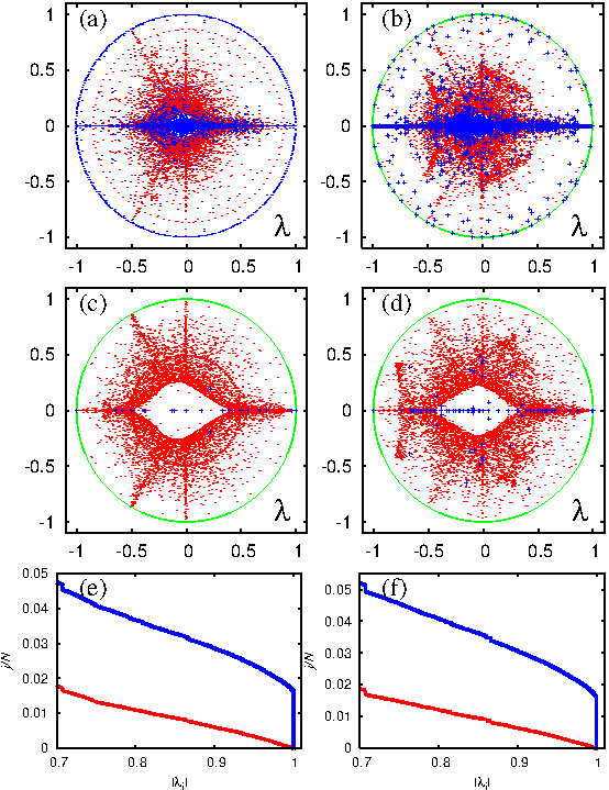
The spectra of all subspace eigenvalues and $n_{A}=20000$ core space eigenvalues of the matrices $S$ and $S^{*}$ are shown in Fig. 17. Even if the decay of PageRank and CheiRank probabilities with rank index is rather similar for both universities (see Fig.1 in Frahm et al. (2011)) the spectra of two networks are very different. Thus the spectrum contains much more detailed information about the network features compared to the rank vectors.

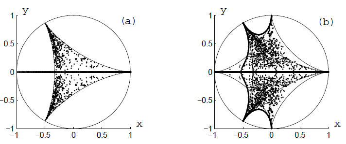
At the same time the spectra of two universities have certain similar features. Indeed, one can identify cross and triple-star structures. These structures are very similar to those seen in the spectra of random orthostochastic matrices of small size $N=3,4$ shown in Fig. 18 from Zyczkowski et al. (2003) (spectra of unistochastic matrices have a similar structure). The spectrum borders, determined analytically in Zyczkowski et al. (2003) for these $N$ values, are also shown. The similarity is more visible for the spectrum of $S^{*}$ case ((c) and (d) of Fig. 17). We attribute this to a larger randomness in outgoing links which have more fluctuations compared to ingoing links, as discussed in Eom et al. (2013b). The similarity of spectra of Fig. 17 with those of random matrices in Fig. 18 indicates that there are dominant triple and quadruple structures of nodes present in the University networks which are relatively weakly connected to other nodes.

Figure 18: Spectra $\lambda$ of 800 random orthostochastic matrices of size $N=3$ (a) and $N=4$ (b) ($Re\lambda=x,Im\lambda=y$). Thin lines denote 3- and 4-hypocycloids, while the thick lines represent the 3-4 interpolation arc. After Zyczkowski et al. (2003).

The core space submatrix $S_{cc}$ of Eq. (2) does not obey to the column sum normalization due to non-vanishing elements in the block $S_{sc}$ which allow for a small but finite escape probability from core space to subspace nodes. Therefore the maximum eigenvalue of the core space (of the matrix $S_{cc}$) is below unity. For Cambridge 2006 (Oxford 2006) it is given by $\lambda^{\rm(core)}_{1}=0.999874353718$ (0.999982435081) with a quite clear gap $1-\lambda^{\rm(core)}_{1}\sim 10^{-4}$ ($\sim 10^{-5}$).

VIII.2 Universal emergence of PageRank

For $\alpha=1$ the leading eigenvalue $\lambda=1$ is highly degenerate due to the subspace structure. This degeneracy is lifted for $\alpha<1$ with a unique eigenvector, the PageRank, for the leading eigenvalue. The question arises how the PageRank emerges if $1-\alpha\ll 1$. Following Frahm et al. (2011), an answer is obtained from a formal matrix expression:

$$P=(1-\alpha)\,(I-\alpha S)^{-1}\,e/N,$$ (8)

where the vector $e$ has unit entries on each node and $I$ is the unit matrix. Then, assuming that $S$ is diagonalizable (with no nontrivial Jordan blocks) we can use the expansion:

$$P=\sum_{\lambda_{j}=1}c_{j}\,\psi_{j}+\sum_{\lambda_{j}\neq 1}\frac{1-\alpha}{(1-\alpha)+\alpha(1-\lambda_{j})}\,c_{j}\,\psi_{j}\ .$$ (9)

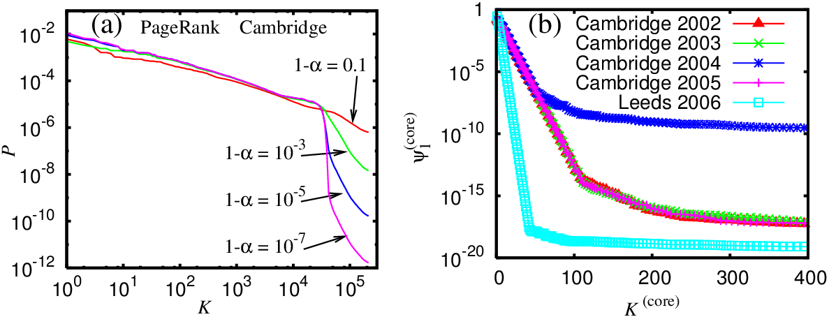
where $\psi_{j}$ are the eigenvectors of $S$ and $c_{j}$ coefficients determined by the expansion $e/N=\sum_{j}c_{j}\psi_{j}$. Thus Eq. (9) indicates that in the limit $\alpha\to 1$ the PageRank converges to a particular linear combination of the eigenvectors with $\lambda_{j}=1$, which are all localized in one of the subspaces. For a finite but very small value of $1-\alpha\ll 1-\lambda_{1}^{\rm(core)}$ the corrections for the contributions of the core space nodes are $\sim(1-\alpha)/(1-\lambda_{1}^{\rm(core)})$. This behavior is indeed confirmed by Fig. 19 (a) showing the evolution of the PageRank for different values of $1-\alpha$ for the case of Cambridge 2006 and using a particular method, based on an alternate combination of the power iteration method and the Arnoldi method Frahm et al. (2011), to determine numerically the PageRank for very small values of $1-\alpha\sim 10^{-8}$.

However, for certain of the university networks the core space gap $1-\lambda_{1}^{\rm(core)}$ is particularly small, for example $1-\lambda_{1}^{\rm(core)}\sim 10^{-17}$, such that in standard double precision arithmetic the Arnoldi method, applied on the matrix $S_{cc}$, does not allow to determine this small gap. For these particular cases it is possible to determine rather accurately the core space gap and the corresponding eigenvector by another numerical approach called “projected power method” Frahm et al. (2011). These eigenvectors, shown in Fig. 19 (b), are strongly localized on a modest number of nodes $\sim 10^{2}$ and with very small but non-vanishing values on the other nodes. Technically these vectors extend to the whole core space but practically they define small quasi-subspaces (in the core space domain) where the escape probability is extremely small Frahm et al. (2011) and in the range $1-\alpha\sim 10^{-8}$ they still contribute to the PageRank according to Eq. (9).

Figure 19: (Color online) (a) PageRank $P(K)$ of Cambridge 2006 for $1-\alpha=0.1,\,10^{-3},\,10^{-5},\,10^{-7}$. (b) First core space eigenvector $\psi_{1}^{\rm(core)}$ versus its rank index $K^{\rm(core)}$ for the UK university networks with a small core space gap $1-\lambda_{1}^{\rm(core)}<10^{-8}$. After Frahm et al. (2011).

Figure 20: (Color online) (a) Fraction of invariant subspaces $F$ with dimensions larger than $d$ as a function of the rescaled variable $x=d/\langle d\rangle$. Upper curves correspond to Cambridge (green/gray) and Oxford (blue/black) for years 2002 to 2006 and middle curves (shifted down by a factor of 10) correspond to the university networks of Glasgow, Cambridge, Oxford, Edinburgh, UCL, Manchester, Leeds, Bristol and Birkbeck for year 2006 with $\langle d\rangle$ between 14 and 31. Lower curve (shifted down by a factor of 100) corresponds to the matrix $S^{*}$ of Wikipedia with $\langle d\rangle=4$. The thick black line is $F(x)=(1+2x)^{-1.5}$. (b) Rescaled PageRank $P\,N_{s}$ versus rescaled rank index $K/N_{s}$ for $1-\alpha=10^{-8}$ and $3974\leq N_{s}\leq 48239$ for the same university networks as in (a) (upper and middle curves, the latter shifted down and left by a factor of 10). The lower curve (shifted down and left by a factor of 100) shows the rescaled CheiRank of Wikipedia $P^{*}\,N_{s}$ versus $K^{*}/N_{s}$ with $N_{s}=21198$. The thick black line corresponds to a power law with exponent $-2/3$. After Frahm et al. (2011).

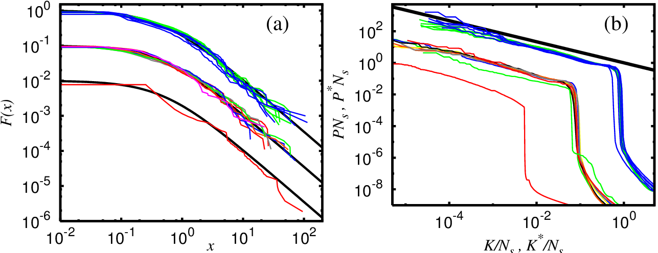
In Fig. 20(b) we show that for several of the university networks the PageRank at $1-\alpha=10^{-8}$ has actually a universal form when using the rescaled variables $P\,N_{s}$ versus $K/N_{s}$ with a power law behavior close to $P\propto K^{-2/3}$ for $K/N_{s}<1$. The rescaled data of Fig. 20 (a) show that the fraction of subspaces with dimensions larger than $d$ is well described by the power law $F(x)\approx(1+2x)^{-1.5}$ with the dimensionless variable $x=d/\langle d\rangle$ where $\langle d\rangle$ is an average subspace dimension computed for WWW of a given university. The tables of all considered UK universities with the parameters of their WWW are given in Frahm et al. (2011). We note that the CheiRank of $S^{*}$ of Wikipedia 2009 also approximately follows the above universal distributions. However, for $S$ matrix of Wikipedia the number of subspaces is small and statistical analysis cannot be performed for this case.

The origin of the universal distribution $F(x)$ still remains a puzzle. Possible links with a percolation on directed networks (see e.g. Dorogovtsev et al. (2008)) are still to be elucidated. It also remains unclear how stable this distribution really is. It works well for UK university networks 2002-2006. However, for the Twitter network Frahm and Shepelyansky (2012b) such a distribution becomes rather approximate. Also for the network of Cambridge in 2011, analyzed in Ermann et al. (2012a, 2013b) with $N\approx 8.9\times 10^{5}$, $N_{\ell}\approx 1.5\times 10^{7}$, the number of subspaces is significantly reduced and a statistical analysis of their size distribution becomes not relevant. It is possible that an increase of number of links per node $N_{\ell}/N$ from a typical value of $10$ for UK universities to $35$ for Twitter affects this distribution. For Cambridge 2011 the network entered in a regime when many links are generated by robots that apparently leads to a change of its statistical properties.

VIII.3 Two-dimensional ranking for University networks

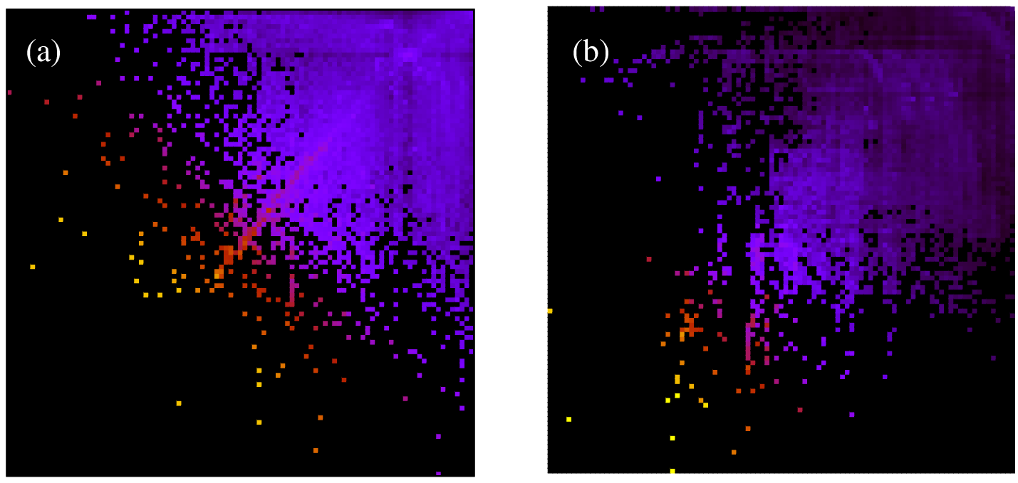
Two-dimensional ranking of network nodes provides a new characterization of directed networks. Here we consider a density distribution of nodes (see Sec. IV.3) in the PageRank-CheiRank plane for examples of two WWW networks of Cambridge 2006 and ENS Paris 2011 shown in Fig. 21 from Ermann et al. (2012a).

The density distribution for Cambridge 2006 clearly shows that nodes with high PageRank have low CheiRank that corresponds to zero density at low $K$, $K^{*}$ values. At large $K$, $K^{*}$ values there is a maximum line of density which is located not very far from the diagonal $K\approx K^{*}$. The presence of correlations between $P(K_{i})$ and $P^{*}({K_{i}}^{*})$ leads to a probability distribution with one main maximum along a diagonal at $\ln K+\ln K^{*}=const$. This is similar to the properties of the density distribution for the Wikipedia network shown in Fig. 7(a).

The 2DRanking might give new possibilities for information retrieval from large databases which are growing rapidly with time. Indeed, for example the size of the Cambridge network increased by a factor 4 from 2006 to 2011. At present, web robots start automatically to generate new web pages. These features can be responsible for the appearance of gaps in the density distribution in $(K,K^{*})$ plane at large $K,K^{*}\sim N$ values visible for large scale university networks such as ENS Paris in 2011 (see Fig. 21). Such an automatic generation of links can change the scale-free properties of networks. Indeed, for ENS Paris a large step in the PageRank distribution appears Ermann et al. (2012a) possibly indicating a delocalization transition tendency of the PageRank that can destroy the efficiency of information retrieval from the WWW.

Figure 21: (Color online) Density distribution $W(K,K^{*})=dN_{i}/dKdK^{*}$ for networks of Universities in the plane of PageRank $K$ and CheiRank $K^{*}$ indexes in log-scale $(\log_{N}K,\log_{N}K^{*})$. The density is shown for $100\times 100$ equidistant grid in $\log_{N}K,\log_{N}K^{*}\in[0,1]$, the density is averaged over all nodes inside each cell of the grid, the normalization condition is $\sum_{K,K^{*}}W(K,K^{*})=1$. Color varies from black for zero to yellow/gray for maximum density value $W_{M}$ with a saturation value of $W_{s}^{1/4}=0.5W_{M}^{1/4}$ so that the same color is fixed for $0.5W_{M}^{1/4}\leq W^{1/4}\leq W_{M}^{1/4}$ to show in a better way low densities. The panels show networks of University of Cambridge 2006 with $N=212710$ (a) and ENS Paris 2011 for crawling level 7 with $N=1820015$ (b). After Ermann et al. (2012a).

IX Wikipedia networks

The free online encyclopedia Wikipedia is a huge repository of human knowledge. Its size is growing permanently accumulating huge amount of information and becoming a modern version of Library of Babel, described by Jorge Luis Borges Borges (1962). The hyperlink citations between Wikipedia articles provides an important example of directed networks evolving in time for many different languages. In particular, the English edition of August 2009 has been studied in detail Zhirov et al. (2010); Ermann et al. (2012a, 2013b). The effects of time evolution Eom et al. (2013b) and entanglement of cultures in multilingual Wikipedia editions have been investigated in Aragón et al. (2012); Eom and Shepelyansky (2013a); Eom et al. (2014).

IX.1 Two-dimensional ranking of Wikipedia articles

The statistical distribution of links in Wikipedia networks has been found to follow a power law with the exponents $\mu_{\rm in},\mu_{\rm out}$ (see e.g. Zlatic et al. (2006); Capocci et al. (2006); Muchnik et al. (2007); Zhirov et al. (2010)). The probabilities of PageRank and CheiRank are shown in Fig. 5. They are satisfactory described by a power law decay with exponents $\beta_{PR,CR}=1/(\mu_{\rm in,out}-1)$ Zhirov et al. (2010).

The density distribution of articles over PageRank-CheiRank plane $(\log_{N}K,\log_{N}K^{*})$ is shown in Fig. 7(a) for English Wikipedia Aug 2009. We stress that the density is very different from those generated by the product of independent probabilities of $P$ and $P^{*}$ given in Fig. 5. In the latter case we obtain a density homogeneous along lines $\ln K^{*}=-\ln K+const$ being rather similar to the distribution for Linux network also shown in Fig. 7. This result is in good agreement with a fact that the correlator $\kappa$ between PageRank and CheiRank vectors is rather large for Wikipedia $\kappa=4.08$ while it is close to zero for Linux network $\kappa\approx-0.05$.

The difference between PageRank and CheiRank is clearly seen from the names of articles with highest ranks (ranks of all articles are given in Zhirov et al. (2010)). At the top of PageRank we have 1. United States, 2. United Kingdom, 3. France while for CheiRank we find 1. Portal:Contents/Outline of knowledge/Geography and places, 2. List of state leaders by year, 3. Portal:Contents/Index/Geography and places. Clearly PageRank selects first articles on a broadly known subject with a large number of ingoing links while CheiRank selects first highly communicative articles with many outgoing links. The 2DRank combines these two characteristics of information flow on directed network. At the top of 2DRank $K_{2}$ we find 1. India, 2. Singapore, 3. Pakistan. Thus, these articles are most known/popular and most communicative at the same time.

The top 100 articles in $K,K_{2},K^{*}$ are determined for several categories including countries, universities, people, physicists. It is shown in Zhirov et al. (2010) that PageRank recovers about 80% of top 100 countries from SJR data base SJR (2007), about 75% of top 100 universities of Shanghai university ranking Shanghai ranking (2010), and, among physicists, about 50% of top 100 Nobel winners in physics. This overlap is lower for 2DRank and even lower for CheiRank. However, as we will see below in more detail, 2DRank and CheiRank highlight other properties being complementary to PageRank.

Let us give an example of top three physicists among those of 754 registered in Wikipedia in 2010: 1. Aristotle, 2. Albert Einstein, 3. Isaac Newton from PageRank; 1. Albert Einstein, 2. Nikola Tesla, 3. Benjamin Franklin from 2DRank; 1. Hubert Reeves, 2. Shen Kuo, 3. Stephen Hawking from CheiRank. It is clear that PageRank gives most known, 2DRank gives most known and active in other areas, CheiRank gives those who are known and contribute to popularization of science. Indeed, e.g. Hubert Reeves and Stephen Hawking are very well known for their popularization of physics that increases their communicative power and place them at the top of CheiRank. Shen Kuo obtained recognized results in an enormous variety of fields of science that leads to the second top position in CheiRank even if his activity was about thousand years ago.

According to Wikipedia ranking the top universities are 1. Harvard University, 2. University of Oxford, 3. University of Cambridge in PageRank; 1. Columbia University, 2. University of Florida, 3. Florida State University in 2DRank and CheiRank. CheiRank and 2DRank highlight connectivity degree of universities that leads to appearance of significant number of arts, religious and military specialized colleges (12% and 13% respectively for CheiRank and 2DRank) while PageRank has only 1% of them. CheiRank and 2DRank introduce also a larger number of relatively small universities who are keeping links to their alumni in a significantly better way that gives an increase of their ranks. It is established Eom et al. (2013b) that top $10$ PageRank universities from English Wikipedia in years $2003,2005,2007,2009,2011$ recover correspondingly $9,9,8,7,7$ from top 10 of Shanghai ranking (2010).

The time evolution of probability distributions of PageRank, CheiRank and two-dimensional ranking is analyzed in Eom et al. (2013b) showing that they become stabilized for the period 2007-2011.

On the basis of these results we can conclude that the above algorithms provide correct and important ranking of huge information and knowledge accumulated at Wikipedia. It is interesting that even Dow-Jones companies are ranked via Wikipedia networks in a good manner Zhirov et al. (2010). We discuss ranking of top people of Wikipedia a bit later.

IX.2 Spectral properties of Wikipedia network

The complex spectrum of eigenvalues of $G$ for English Wikipedia network of Aug 2009 is shown in Fig. 22. As for university networks, the spectrum also has some invariant subspaces resulting in degeneracies of the leading eigenvalue $\lambda=1$ of $S$ (or $S^{*}$). However, due to the stronger connectivity of the Wikipedia network these subspaces are significantly smaller compared to university networks Ermann et al. (2013b); Eom et al. (2013b). For example of Aug 2009 edition in Fig. 22 there are $255$ invariant subspaces (of the matrix $S$) covering $515$ nodes with $255$ unit eigenvalues $\lambda_{j}=1$ and $381$ eigenvalues on the complex unit circle with $|\lambda_{j}|=1$. For the matrix $S^{*}$ of Wikipedia there are $5355$ invariant subspaces with $21198$ nodes, $5365$ unit eigenvalues and 8968 eigenvalues on the unit circle Ermann et al. (2013b). The complex spectra of all subspace eigenvalues and the first $n_{A}=6000$ core space eigenvalues of $S$ and $S^{*}$ are shown in Fig. 22. As in the university cases, in the spectrum we can identify cross and triple-star structures similar to those of orthostochastic matrices shown in Fig. 18. However, for Wikipedia (especially for $S$) the largest complex eigenvalues outside the real axis are more far away from the unit circle. For $S$ of Wikipedia the two largest core space eigenvalues are $\lambda^{\rm(core)}_{1}=0.999987$ and $\lambda^{\rm(core)}_{2}=0.977237$ indicating that the core space gap $|1-\lambda^{\rm(core)}_{1}|\sim 10^{-5}$ is much smaller than the secondary gap $|\lambda^{\rm(core)}_{1}-\lambda^{\rm(core)}_{2}|\sim 10^{-2}$. As a consequence the PageRank of Wikipedia (at $\alpha=0.85$) is strongly influenced by the leading core space eigenvector and actually both vectors select the same 5 top nodes.

The time evolution of spectra of $G$ and $G^{*}$ for English Wikipedia is studied in Eom et al. (2013b). It is shown that the spectral structure remains stable for years 2007 - 2011.

Figure 22: (Color online) Complex eigenvalue spectra $\lambda$ of $S$ (a) and $S^{*}$ (b) for English Wikipedia of Aug 2009 with $N=3282257$ articles and $N_{\ell}=71012307$ links. Red/gray dots are core space eigenvalues, blue/black dots are subspace eigenvalues and the full green/gray curve shows the unit circle. The core space eigenvalues are computed by the projected Arnoldi method with Arnoldi dimension $n_{A}=6000$. After Eom et al. (2013b).

Figure 23: (Color online) Complex eigenvalue spectrum of the matrices $S$ for English Wikipedia Aug 2009. Highlighted eigenvalues represent different communities of Wikipedia and are labeled by the most repeated and important words following word counting of first 1000 nodes. Panel (a) shows complex plane for positive imaginary part of eigenvalues, while panels (b) and (c) zoom in the negative and positive real parts. After Ermann et al. (2013b).

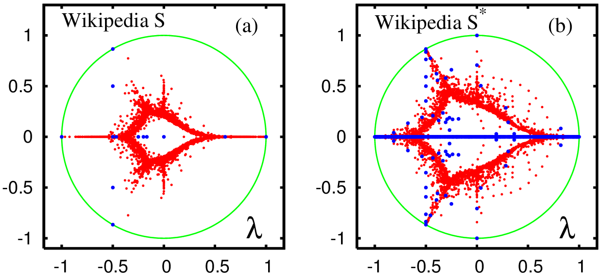
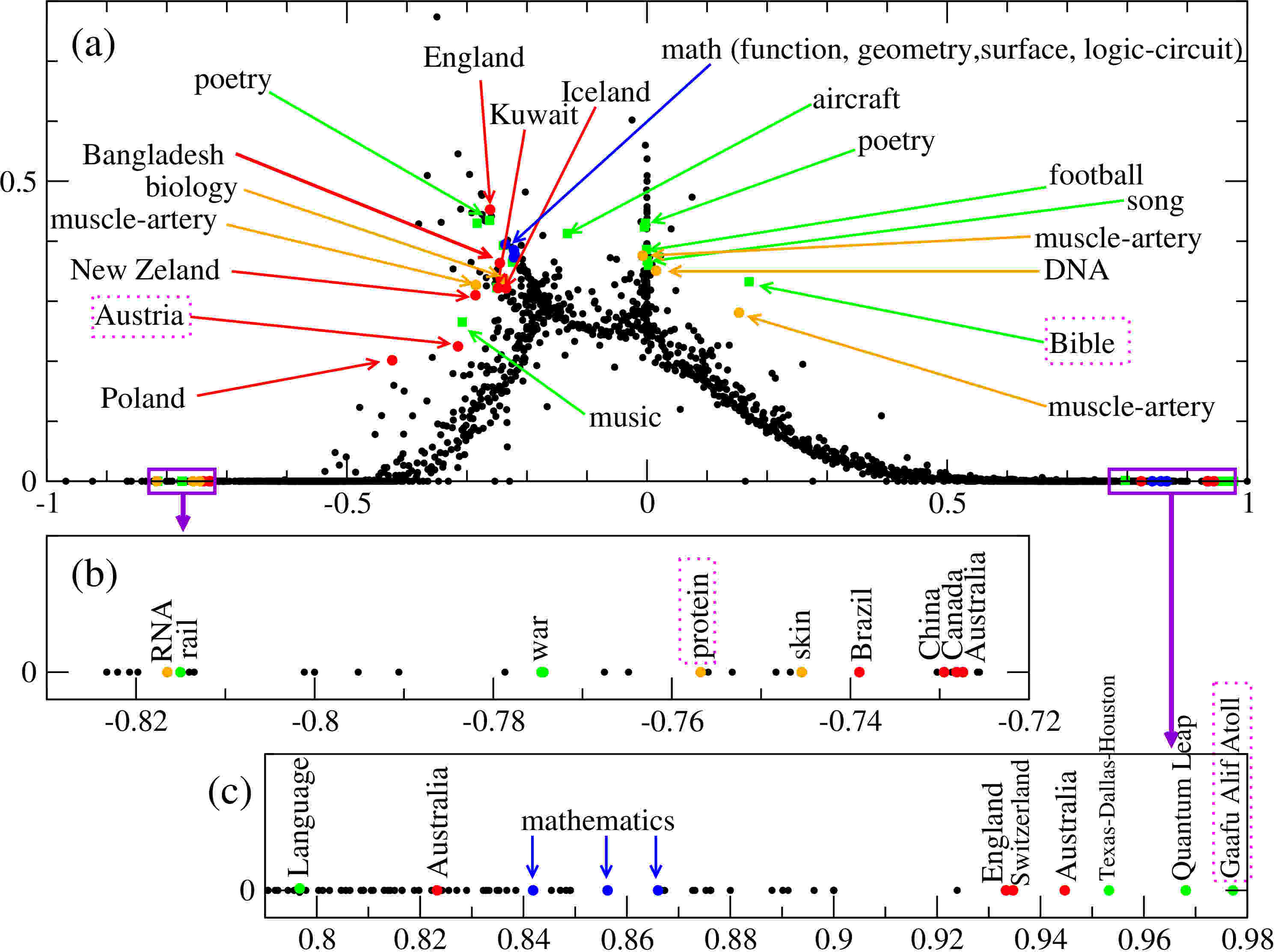
IX.3 Communities and eigenstates of Google matrix

The properties of eigenstates of Gogle matrix of Wikipedia Aug 2009 are analyzed in Ermann et al. (2013b). The global idea is that the eigenstates with large values of $|\lambda|$ select certain specific communities. If $|\lambda|$ is close to unity then a relaxation of probability from such nodes is rather slow and we can expect that such eigenstates highlight some new interesting information even if these nodes are located on a tail of PageRank. The important advantage of the Wikipedia network is that its nodes are Wikipedia articles with a relatively clear meaning allowing to understand the origins of appearance of certain nodes in one community.

The localization properties of eigenvectors $\psi_{i}$ of the Google matrix can be analyzed with the help of IPR $\xi$ (see Sec. III.5). Another possibility is to fit a decay of an eigenstate amplitude by a power law $|\psi_{i}(K_{i})|\sim\,K_{i}^{b}$ where $K_{i}$ is the index ordering $|\psi_{i}(j)|$ by monotonically decreasing amplitude (similar to $P(K)$ for PageRank). The exponents $b$ on the tails of $|\psi_{i}(j)|$ are found to be typically in the range $-2<b<-1$ Ermann et al. (2013b). At the same time the eigenvectors with large complex eigenvalues or real eigenvalues close to $\pm 1$ are quite well localized on $\xi_{i}\approx 10^{2}-10^{3}$ nodes that is much smaller than the whole network size $N\approx 3\times 10^{6}$.

To understand the meaning of other eigenstates in the core space we order selected eigenstates by their decreasing value $|\psi_{i}(j)|$ and apply word frequency analysis for the first $1000$ articles with $K_{i}\leq 1000$. The mostly frequent word of a given eigenvector is used to label the eigenvector name. These labels with corresponding eigenvalues are shown in Fig. 23. There are four main categories for the selected eigenvectors belonging to countries (red/gray), biology and medicine (orange/very light gray), mathematics (blue/black) and others (green/light gray). The category of others contains rather diverse articles about poetry, Bible, football, music, American TV series (e.g. Quantum Leap), small geographical places (e.g. Gaafru Alif Atoll). Clearly these eigenstates select certain specific communities which are relatively weakly coupled with the main bulk part of Wikipedia that generates relatively large modulus of $|\lambda_{i}|$.

For example, for the article Gaafu Alif Atoll the eigenvector is mainly localized on names of small atolls forming Gaafu Alif Atoll. Clearly this case represents well localized community of articles mainly linked between themselves that gives slow relaxation rate of this eigenmode with $\lambda=0.9772$ being rather close to unity. Another eigenvector has a complex eigenvalue with $|\lambda|=0.3733$ and the top article Portal:Bible. Another two articles are Portal:Bible/Featured chapter/archives, Portal:Bible/Featured article. These top $3$ articles have very close values of $|\psi_{i}(j)|$ that seems to be the reason why we have $\varphi=\arg(\lambda_{i})=0.3496\pi$ being very close to $\pi/3$. Examples of other eigenvectors are discussed in Ermann et al. (2013b) in detail.

The analysis performed in Ermann et al. (2013b) for Wikipedia Aug 2009 shows that the eigenvectors of the Google matrix of Wikipedia clearly identify certain communities which are relatively weakly connected with the Wikipedia core when the modulus of corresponding eigenvalue is close to unity. For moderate values of $|\lambda|$ we still have well defined communities which are however have stronger links with some popular articles (e.g. countries) that leads to a more rapid decay of such eigenmodes. Thus the eigenvectors highlight interesting features of communities and network structure. However, a priori, it is not evident what is a correspondence between the numerically obtained eigenvectors and the specific community features in which someone has a specific interest. In fact, practically each eigenvector with a moderate value $|\lambda|\sim 0.5$ selects a certain community and there are many of them. So it remains difficult to target and select from eigenvalues $\lambda$ a specific community one is interested.

The spectra and eigenstates of other networks like WWW of Cambridge 2011, Le Monde, BBC and PCN of Python are discussed in Ermann et al. (2013b). It is found that IPR values of eigenstates with large $|\lambda|$ are well localized with $\xi\ll N$. The spectra of each network have significant differences from one another.

IX.4 Top people of Wikipedia

There is always a significant public interest to know who are most significant historical figures, or persons, of humanity. The Hart list of the top 100 people who, according to him, most influenced human history, is available at Hart (1992). Hart “ranked these 100 persons in order of importance: that is, according to the total amount of influence that each of them had on human history and on the everyday lives of other human beings” Hart (1992). Of course, a human ranking can be always objected arguing that an investigator has its own preferences. Also investigators from different cultures can have different view points on a same historical figure. Thus it is important to perform ranking of historical figures on purely mathematical and statistical grounds which exclude any cultural and personal preferences of investigators.

A detailed two-dimensional ranking of persons of English Wikipedia Aug 2009 has been done in Zhirov et al. (2010). Earlier studies had been done in a non-systematic way without any comparison with established top $100$ lists (see these Refs. in Zhirov et al. (2010); Wikipedia Top 100 (2014)). Also at those times Wikipedia did not yet entered in its stabilized phase of development.

The top people of Wikipedia Aug 2009 are found to be 1. Napoleon I of France, 2. George W. Bush, 3. Elizabeth II of the United Kingdom for PageRank; 1.Michael Jackson, 2. Frank Lloyd Wright, 3. David Bowie for 2DRank; 1. Kasey S. Pipes, 2. Roger Calmel, 3. Yury G. Chernavsky for CheiRank Zhirov et al. (2010). For the PageRank list of $100$ the overlap with the Hart list is at 35% (PageRank), 10% (2DRank) and almost zero for CheiRank. This is attributed to a very broad distribution of historical figures on 2D plane, as shown in Fig. 7, and a large variety of human activities. These activities are classified by $5$ main categories: politics, religion, arts, science, sport. For the top $100$ PageRank persons we have the following distribution over these categories: $58$, $10$, $17$, $15$, $0$ respectively. Clearly PageRank overestimates the significance of politicians which list is dominated by USA presidents not always much known to a broad public. For 2DRank we find respectively $24$, $5$, $62$, $7$, $2$. Thus this rank highlights artistic sides of human activity. For CheiRank we have $15$, $1$, $52$, $16$, $16$ so that the dominant contribution comes from arts, science and sport. The interesting property of this rank is that it selects many composers, singers, writers, actors. As an interesting feature of CheiRank we note that among scientists it selects those who are not so much known to a broad public but who discovered new objects, e.g. George Lyell who discovered many Australian butterflies or Nikolai Chernykh who discovered many asteroids. CheiRank also selects persons active in several categories of human activity.

For English Wikipedia Aug 2009 the distribution of top 100 PageRank, CheiRank and Hart’s persons on PageRank-CheiRank plane is shown in Fig. 7 (a).

The distribution of Hart’s top $100$ persons on $(K,K^{*})$ plane for English Wikipedia in years 2003, 2005, 2007, Aug 2009, Dec 2009, 2011 is found to be stable for the period 2007-2011 even if certain persons change their ranks Eom et al. (2013b). The distribution of top $100$ persons of Wikipedia Aug 2009 remains stable and compact for PageRank and 2DRank for the period 2007-2011 while for CheiRank the fluctuations of positions are large. This is due to the fact that outgoing links are easily modified and fluctuating.

The time evolution of distribution of top persons over fields of human activity is established in Eom et al. (2013b). PageRank persons are dominated by politicians whose percentage increases with time, while the percent of arts decreases. For 2DRank the arts are dominant but their percentage decreases with time. We also see the appearance of sport which is absent in PageRank. The mechanism of the qualitative ranking differences between two ranks is related to the fact that 2DRank takes into account via CheiRank a contribution of outgoing links. Due to that singers, actors, sportsmen improve their CheiRank and 2DRrank positions since articles about them contain various music albums, movies and sport competitions with many outgoing links. Due to that the component of arts gets higher positions in 2DRank in contrast to dominance of politics in PageRank.

The interest to ranking of people via Wikipedia network is growing, as shows the recent study of English edition Skiena and Ward (2014).

IX.5 Multilingual Wikipedia editions

The English edition allows to obtain ranking of historical people but as we saw the PageRank list is dominated by USA presidents that probably does not correspond to the global world view point. Hence, it is important to study multilingual Wikipedia editions which have now $287$ languages and represent broader cultural views of the world.

One of the first cross-cultural study was done for $15$ largest language editions constructing a network of links between set of articles of people biographies for each edition. However, the number of nodes and links in such a biographical network is significantly smaller compared to the whole network of Wikipedia articles and thus the fluctuations become rather large. For example, from the biographical network of the Russian edition one finds as the top person Napoleon III (and even not Napoleon I) Aragón et al. (2012), who has a rather low importance for Russia.

Another approach was used in Eom and Shepelyansky (2013a) ranking top 30 persons by PageRank, 2DRank and CheiRank algorithms for all articles of each of 9 editions and attributing each person to her/his native language. The selected editions are English (EN), French (FR), German (DE), Italian (IT), Spanish (ES), Dutch (NL), Russian (RU), Hungarian (HU) and Korean (KO). The aim here is to understand how different cultures evaluate a person? Is an important person in one culture is also important in the other culture? It is found that local heroes are dominant but also global heroes exist and create an effective network representing entanglement of cultures.

The top article of PageRank is usually USA or the name of country of a given language (FR, RU, KO). For NL we have at the top beetle, species, France. The top articles of CheiRank are various listings.

The distributions of articles density and top 30 persons for each rank algorithm are shown in Fig. 24 for four editions EN, FR, DE, RU. We see that in global the distributions have a similar shape that can be attributed to a fact that all editions describe the same world. However, local features of distributions are different corresponding to different cultural views on the same world (other 5 editions are shown in Fig.2 in Eom and Shepelyansky (2013a)). The top 30 persons for each edition are selected manually that represents a weak point of this study.

From the lists of top persons, the ”fields” of activity are identified for each top 30 rank persons in which he/she is active on. The six activity fields are: politics, art, science, religion, sport and etc (here “etc” includes all other activities). As shown in Fig. 25, for PageRank, politics is dominant and science is secondarily dominant. The only exception is Dutch where science is the almost dominant activity field (politics has the same number of points). In case of 2DRank in Fig. 25, art becomes dominant and politics is secondarily dominant. In case of CheiRank, art and sport are dominant fields (see Fig.3 in Eom and Shepelyansky (2013a)). Thus for example, in CheiRank top 30 list we find astronomers who discovered a lot of asteroids, e.g. Karl Wilhelm Reinmuth (4th position in RU and 7th in DE), who was a prolific discoverer of about 400 of them. As a result, his article contains a long listing of asteroids discovered by him and giving him a high CheiRank. The distributions of persons over activity fields are shown in Fig. 25 for 9 languages editions (marked by standard two letters used by Wikipedia).

Figure 24: (Color online) Density of Wikipedia articles in the PageRank-CheiRank plane $(K,K^{*})$ for four different language Wikipedia editions. The red (gray) points are top PageRank articles of persons, the green (light gray) squares are top 2DRank articles of persons and the cyan (dark gray) triangles are top CheiRank articles of persons. Wikipedia language editions are English EN (a), French FR (b), German DE (c), and Russian RU (d). Color bars show natural logarithm of density, changing from minimal nonzero density (dark) to maximal one (white), zero density is shown by black. After Eom and Shepelyansky (2013a).

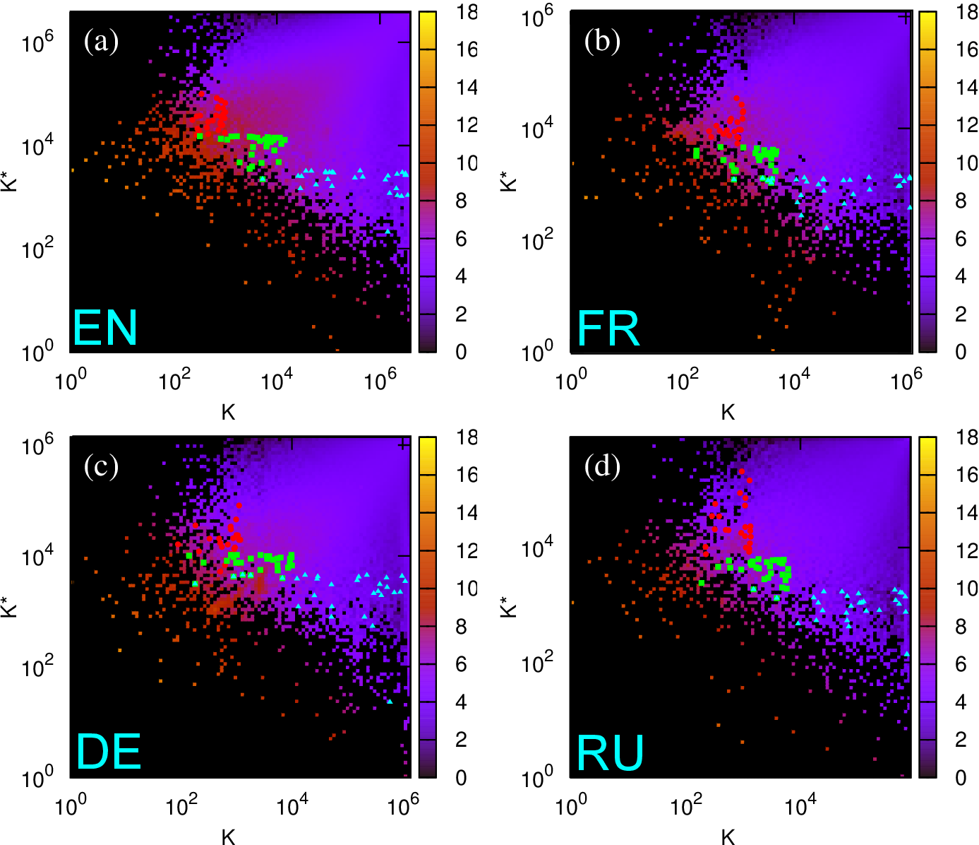
The change of activity priority for different ranks is due to the different balance between incoming and outgoing links there. Usually the politicians are well known for a broad public, hence, the articles about politicians are pointed by many articles. However, the articles about politicians are not very communicative since they rarely point to other articles. In contrast, articles about persons in other fields like science, art and sport are more communicative because of listings of insects, planets, asteroids they discovered, or listings of song albums or sport competitions they gain.

On the basis of this approach one obtains local ranks of each of 30 persons $1\leq K_{P,E,A}\leq 30$ for each edition $E$ and algorithm $A$. Then an average ranking score of a person $P$ is determined as $\Theta_{P,A}=\sum_{E}(31-K_{P,E,A})$ for each algorithm. This method determines the global historical figures. The top global persons are 1.Napoleon, 2.Jesus, 3.Carl Linnaeus for PageRank; 1.Micheal Jackson , 2.Adolf Hitler, 3.Julius Caesar for 2DRank. For CheiRank the lists of different editions have rather low overlap and such an averaging is not efficient. The first positions reproduce top persons from English edition discussed in Sec. IX.4, however, the next ones are different.

Figure 25: (Color online) Distribution of top 30 persons over activity fields for PageRank $(a)$ and 2DRank $(b)$ for each of 9 Wikipedia editions. The color bar shows the values in percent. After Eom and Shepelyansky (2013a).

Figure 26: Number of appearances of historical figures of a given country, obtained from 24 lists of top 100 persons of PageRank (a) and 2DRank (b), shown on the world map. Color changes from zero (white) to maximum (black), it corresponds to average number of person appearances per country. After Eom et al. (2014).

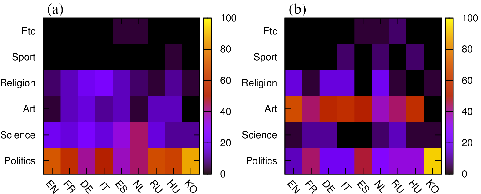
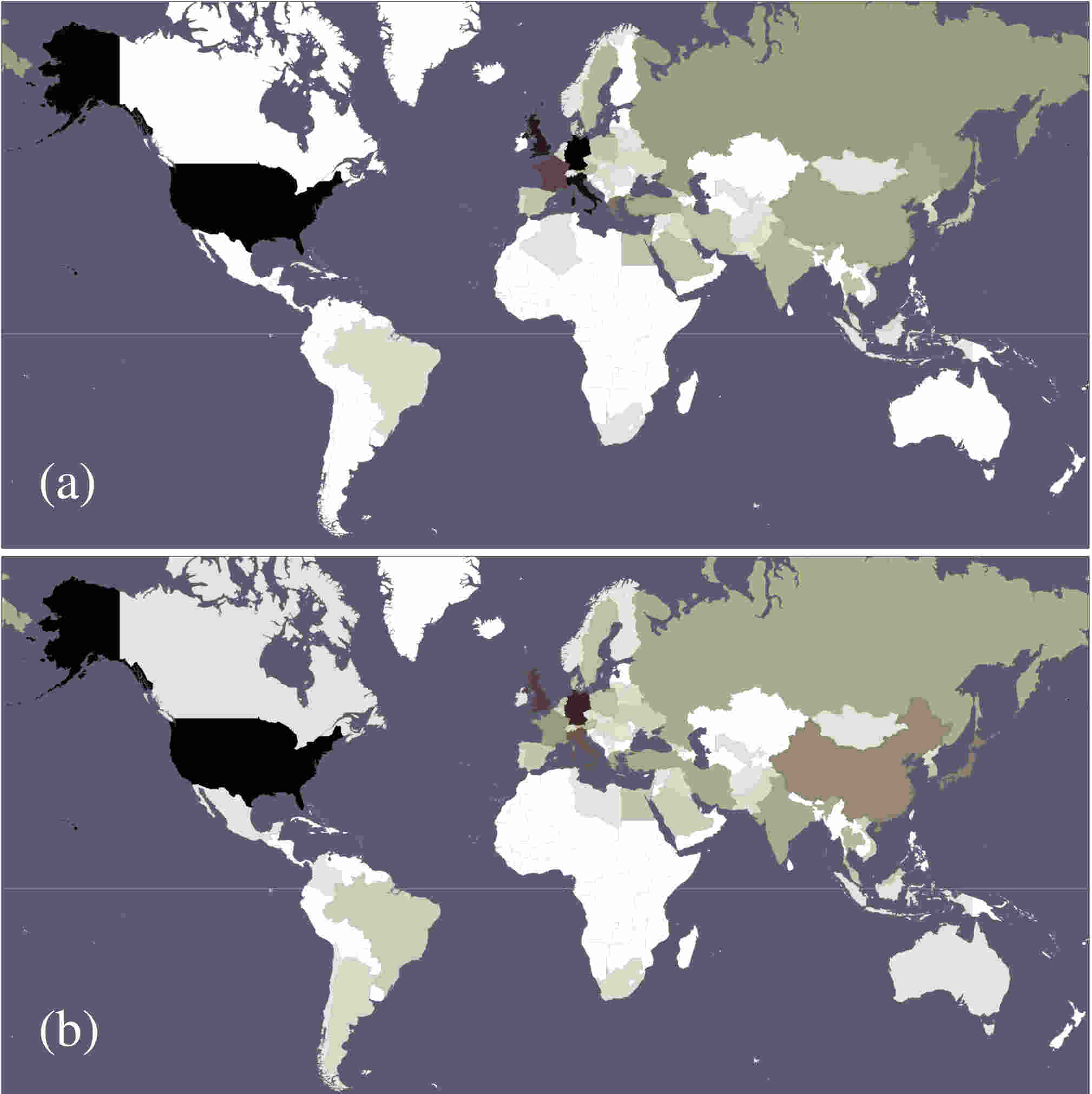
Since each person is attributed to her/his native language it is also possible for each edition to obtain top local heroes who have native language of the edition. For example, we find for PageRank for EN George W. Bush, Barack Obama, Elizabeth II; for FR Napoleon, Louis XIV of France, Charles de Gaulle; for DE Adolf Hitler, Martin Luther, Immanuel Kant; for RU Peter the Great, Joseph Stalin, Alexander Pushkin. For 2DRank we have for EN Frank Sinatra, Paul McCartney, Michael Jackson; for FR Francois Mitterrand, Jacques Chirac, Honore de Balzac; for DE Adolf Hitler, Otto von Bismarck, Ludwig van Beethoven; for RU Dmitri Mendeleev, Peter the Great, Yaroslav the Wise. These ranking results are rather reasonable for each language. Results for other editions and CheiRank are given in Eom and Shepelyansky (2013a).

A weak point of above study is a manual selection of persons and a not very large number of editions. A significant improvement has been reached in a recent study Eom et al. (2014) where 24 editions have been analyzed. These 24 languages cover 59 percent of world population, and these 24 editions covers 68 percent of the total number of Wikipedia articles in all 287 available languages. Also the selection of people from the rank list of each edition is now done in an automatic computerized way. For that a list of about 1.1 million biographical articles about people with their English names is generated. From this list of persons, with their biographical article title in the English Wikipedia, the corresponding titles in other language editions are determined using the inter-language links provided by Wikipedia.

Using the corresponding articles, identified by the inter-languages links in different language editions, the top 100 persons are obtained from the rankings of all Wikipedia articles of each edition. A birth place, birth date, and gender of each top 100 ranked person are identified, based on DBpedia or a manual inspection of the corresponding Wikipedia biographical article, when for the considered person no DBpedia data were available. In this way 24 lists of top 100 persons for each edition are obtained in PageRank with 1045 unique names and in 2DRank with 1616 unique names. Each of the 100 historical figures is attributed to a birth place at the country level, to a birth date in year, to a gender, and to a cultural language group. The birth place is assigned according to the current country borders. The cultural group of historical figures is assigned by the most spoken language of their birth place at the current country level. The considered editions are: English EN, Dutch NL, German DE, French FR, Spanish, ES, Italian IT, Potuguese PT, Greek, EL, Danish DA, Swedish SV, Polish PL, Hungarian HU, Russian RU, Hebrew HE, Turkish TR, Arabic AR, Persian FA, Hindi HI, Malaysian MS, Thai TH, Vietnamese VI, Chinese ZH, Korean KO, Japanese JA (dated by February 2013). The size of network changes from maximal value $N=4212493$ for EN to minimal one $N=78953$ for TH.

All persons are ranked by their average rank score $\Theta_{P,A}=\sum_{E}(101-K_{P,E,A})$ with $1\leq K_{P,E,A}\leq 100$ similar to the study of 9 editions described above. For PageRank the top global historical figures are Carl Linnaeus, Jesus, Aristotle and for 2DRank we obtain Adolf Hitler, Michael Jackson, Madonna (entertainer). Thus the averaging over 24 editions modifies the top ranking. The list of top 100 PageRank global persons has overlap of 43 persons with the Hart list Hart (1992). Thus the averaging over 24 editions gives a significant improvement compared to 35 persons overlap for the case of English edition only Zhirov et al. (2010). For comparison we note that the top 100 list of historical figures has been also determined recently by Pantheon MIT project (2014) having overlap of 42 persons with the Hart list. This Pantheon MIT list is established on the basis of number of editions and number of clicks on an article of a given person without using rank algorithms discussed here. The overlap between top 100 PageRank list and top 100 Pantheon list is 44 percent. More data are available in Eom et al. (2014).

The fact that Carl Linnaeus is the top historical figure of Wikipedia PageRank list came out as a surprise for media and broad public (see Wikipedia Top 100 (2014)). This ranking is due to the fact that Carl Linnaeus created a classification of world species including, animals, insects, herbs, trees etc. Thus all articles of these species point to the article Carl Linnaeus in various languages. As a result Carl Linnaeus appears on almost top positions in all 24 languages. Hence, even if a politician, like Barak Obama, takes the second position in his country language EN (Napoleon is at the first position in EN) he is usually placed at low ranking in other language editions. As a result Carl Linnaeus takes the first global PageRank position.

The number of appearances of historical persons in 24 lists of top 100 for each edition can be distributed over present world countries according to the birth place of each person. This geographical distribution is shown in Fig. 26 for PageRank and 2DRank. In PageRank the top countries are DE, USA, IT and in 2DRank US, DE, UK. The appearance of many UK and US singers improves the positions of English speaking countries in 2DRank.

Figure 27: (Color online) Birth date distributions over $35$ centuries of top historical figures from each Wikipedia edition marked by two letters standard notation of Wikipedia. Panels: (a) column normalized birth date distributions of PageRank historical figures; (b) same as (a) for 2DRank historical figures. After Eom et al. (2014).

The distributions of the top PageRank and 2DRank historical figures over 24 Wikipedia editions for each century are shown in Fig. 27. Each person is attributed to a century according to the birth date covering the range of $35$ centuries from BC 15th to AD 20th centuries. For each century the number of persons for each century is normalized to unity to see more clearly relative contribution of each language for each century.

The Greek edition has more historical figures in BC 5th century because of Greek philosophers. Also most of western-southern European language editions, including English, Dutch, German, French, Spanish, Italian, Portuguese, and Greek, have more top historical figures because they have Augustine the Hippo and Justinian I in common. The Persian (FA) and the Arabic (AR) Wikipedia have more historical figures comparing to other language editions (in particular European language editions) from the 6th to the 12th century that is due to Islamic leaders and scholars. The data of Fig. 27 clearly show well pronounced patterns, corresponding to strong interactions between cultures: from BC 5th century to AD 15th century for JA, KO, ZH, VI; from AD 6th century to AD 12th century for FA, AR; and a common birth pattern in EN,EL,PT,IT,ES,DE,NL (Western European languages) from BC 5th century to AD 6th century. A detailed analysis shows that even in BC 20th century each edition has a significant fraction of persons of its own language so that even with on going globalization there is a significant dominance of local historical figures for certain cultures. More data on the above points and gender distributions are available in Eom et al. (2014).

IX.6 Networks and entanglement of cultures

We now know how a person of a given language is ranked by editions of other languages. Therefore, if a top person from a language edition $A$ appears in another edition $B$, we can consider this as a ’cultural’ influence from culture $A$ to $B$. This generates entanglement in a network of cultures. Here we associate a language edition with its corresponding culture considering that a language is a first element of culture, even if a culture is not reduced only to a language. In Eom and Shepelyansky (2013a) a person is attributed to a given language, or culture, according to her/his native language fixed via corresponding Wikipedia article. In Eom et al. (2014) the attribution to a culture is done via a birth place of a person, each language is considered as a proxy for a cultural group and a person is assigned to one of these cultural groups based on the most spoken language of her/his birth place at the country level. If a person does not belong to any of studied editions then he/she is attributed to an additional cultural group world WR.

After such an attributions of all persons the two networks of cultures are constructed based on the top PageRank historical figures and top 2DRank historical figures respectively. Each culture (i.e. language) is represented as a node of the network, and the weight of a directed link from culture $A$ to culture $B$ is given by the number of historical figures belonging to culture $B$ (e.g. French) appearing in the list of top 100 historical figures for a given culture $A$ (e.g. English).

For example, according to Eom et al. (2014), there are 5 French historical figures among the top 100 PageRank historical figures of the English Wikipedia, so we can assign weight 5 to the link from English to French. Thus, Fig. 28(a) and Fig. 28(b) represent the constructed networks of cultures defined by appearances of the top PageRank historical figures and top 2DRank historical figures, respectively.

In total we have two networks with 25 nodes which include our 24 editions and an additional node WR for all other world cultures. Persons of a given culture are not taken into account in the rank list of language edition of this culture. Then following the standard rules (1) the Google matrix of network of cultures is constructed by normalization of sum of all elements in each column to unity. The matrix $G_{KK^{\prime}}$, written in the PageRank indexes $K,K^{\prime}$ is shown in Fig. 29 for persons from PageRank $(a)$ and 2DRank $(b)$ lists. The matrix $G^{*}$ is constructed in the same way as $G$ for the network with inverted directions of links.

Figure 28: (Color online) Network of cultures, obtained from 24 Wikipedia languages and the remaining world (WR), considering (a) top 100 PageRank historical figures and (b) top 100 2DRank historical figures. The link width and darkness are proportional to a number of foreign historical figures quoted in top 100 of a given culture, the link direction goes from a given culture to cultures of quoted foreign historical figures, quotations inside cultures are not considered. The size of nodes is proportional to their PageRank. After Eom et al. (2014).

Figure 29: (Color online) Google matrix of network of cultures shown in Fig 28 (a) and (b) respectively. The matrix elements $G_{ij}$ are shown by color with damping factor $\alpha=0.85$. After Eom et al. (2014).

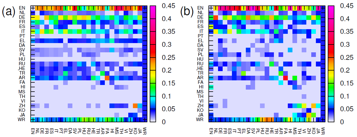
From the obtained matrix $G$ and $G^{*}$ we determine PageRank and CheiRank vectors and then the PageRank-CheiRank plane $(K,K^{*})$, shown in Fig. 30, for networks of cultures from Fig. 28. Here $K$ indicates the ranking of a given culture ordered by how many of its own top historical figures appear in other Wikipedia editions, and $K^{*}$ indicates the ranking of a given culture according to how many of the top historical figures in the considered culture are from other cultures. It is important to note that for 24 editions the world node WR appears on positions $K=3$ or $K=4$, for panels $(a),(b)$ in Fig. 30, signifying that the 24 editions capture the main part of historical figures born in these cultures. We note that for 9 editions in Eom and Shepelyansky (2013a) the node WR was at the top position for PageRank so that a significant fraction of historical figures was attributed to other cultures.

Figure 30: (Color online) PageRank-CheiRank plane of cultures with corresponding indexes $K$ and $K^{*}$ obtained from the network of cultures based on (a) top 100 PageRank historical figures, (b) top 100 2DRank historical figures. After Eom et al. (2014).

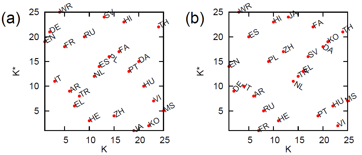
From the data of Fig. 30 we obtain at the top positions of $K$ cultures EN, DE, IT showing that other cultures strongly point to them. However, we can argue that for cultures it is also important to have strong communicative property and hence it is important to have 2DRank of cultures at top positions. On the top 2DRank position we have Greek, Turkish and Arabic (for PageRank persons) in Fig. 30(a) and French, Russian and Arabic (for 2DRank persons) in Fig. 30(b). This demonstrates the important historical influence of these cultures both via importance (incoming links) and communicative (outgoing links) properties present in a balanced manner.

Thus the described research across Wikipedia language editions suggests a rigorous mathematical way, based on Markov chains and Google matrix, for recognition of important historical figures and analysis of interactions of cultures at different historical periods and in different world regions. Such an approach recovers 43 percent of persons from the well established Hart historical study Hart (1992), that demonstrates the reliability of this method. We think that a further extension of this approach to a larger number of Wikipedia editions will provide a more detailed and balanced analysis of interactions of world cultures.

X Google matrix of social networks

Social networks like Facebook, LiveJournal, Twitter, Vkontakte start to play a more and more important role in modern society. The Twitter network is a directed one and here we consider its spectral properties following mainly the analysis reported in Frahm and Shepelyansky (2012b).

X.1 Twitter network

Twitter is a rapidly growing online directed social network. For July 2009 a data set of this entire network is available with $N=41652230$ nodes and $N_{\ell}=1468365182$ links (for data sets see Refs. in Frahm and Shepelyansky (2012b)). For this case the spectrum and eigenstate properties of the corresponding Google matrix have been analyzed in detail using the Arnoldi method and standard PageRank and CheiRank computations Frahm and Shepelyansky (2012b). For the Twitter network the average number of links per node $\zeta=N_{\ell}/N\approx 35$ and the general inter-connectivity between top PageRank nodes are considerably larger than for other networks such as Wikipedia (Sec. IX) or UK universities (Sec. VIII) as can be seen in Figs. 31 and 32.

Figure 31: (Color online) Panel (a): Google matrix of Twitter, matrix elements of $G$ are shown in the basis of PageRank index $K$ of matrix $G_{KK^{\prime}}$. Here, $x$ (and $y$) axis show $K$ (and $K^{{}^{\prime}}$) with the range $1\leq K,K^{\prime}\leq 200$. Panel (b) shows the density of nodes $W(K,K^{*})$ of Twitter on PageRank-CheiRank plane $(K,K^{*})$, averaged over $100\times 100$ logarithmically equidistant grids for $0\leq\ln K,\ln K^{*}\leq\ln N$ with the normalization condition $\sum_{K,K^{*}}W(K,K^{*})=1$. The $x$-axis corresponds to $\ln K$ and the $y$-axis to $\ln K^{*}$. In both panels color varies from blue/black at minimal value to red/gray at maximal value; here $\alpha=0.85$. After Frahm and Shepelyansky (2012b).

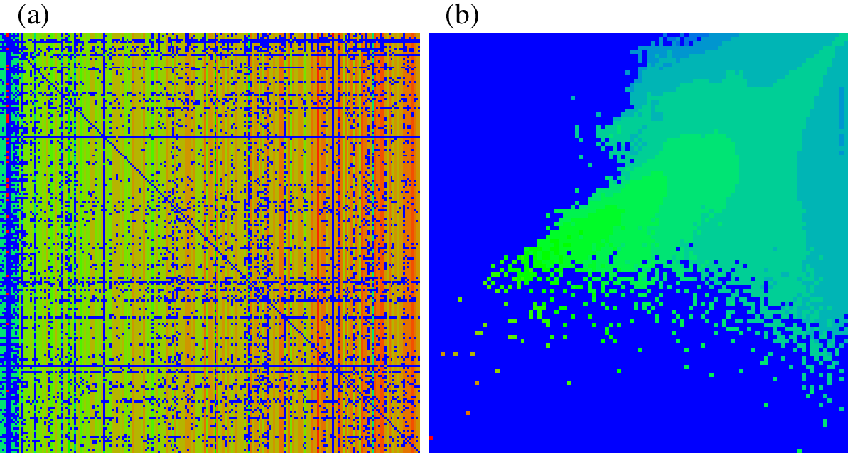
The decay of PageRank probability can be approximately described by an algebraic decay with the exponent $\beta\approx 0.54$ while for CheiRank we have a larger value $\beta\approx 0.86$ Frahm and Shepelyansky (2012b) that is opposite to the usual situation. The image of top matrix elements of $G_{KK^{\prime}}$ with $1\leq K,K;\leq 200$ is shown in Fig. 31. The density distribution of nodes on $(K,K^{*})$ plane is also shown there. It is somewhat similar to those of Wikipedia case in Fig. 24, may be with a larger density concentration along the line $K\approx K^{*}$.

However, the most striking feature of $G$ matrix elements is a very strong inteconnectivity between top PageRank nodes. Thus for Twitter the top $K\leq 1000$ elements fill about 70% of the matrix and about 20% for size $K\leq 10^{4}$ . For Wikipedia the filling factor is smaller by a factor $10-20$. In particular the number $N_{G}$ of links between $K$ top PageRank nodes behaves for $K\leq 10^{3}$ as $N_{G}\sim K^{1.993}$ while for Wikipedia $N_{G}\sim K^{1.469}$. The exponent for $N_{G}$, being close to 2 for Twitter, indicates that for the top PageRank nodes the Google matrix is macroscopically filled with a fraction $0.6-0.8$ of non-vanishing matrix elements (see also Figs. 31 and 32) and the very well connected top PageRank nodes can be considered as the Twitter elite Kandiah and Shepelyansky (2012). For Wikipedia the interconnectivity among top PageRank nodes has an exponent $1.5$ being somewhat reduced but still stronger as compared to certain university networks where typical exponents are close to unity (for the range $10^{2}\leq K\leq 10^{4}$). The strong interconnectivity of Twitter is also visible in its global logarithmic density distribution of nodes in the PageRank-CheiRank plane $(K,K^{*})$ (Fig. 31 (b)) which shows a maximal density along a certain ridge along a line $\ln K^{*}=\ln K+\,$const. with a significant large number of nodes at small values $K,K^{*}<1000$.

Figure 32: (Color online) (a) Dependence of the area density $g_{K}=N_{G}/K^{2}$ of nonzero elements of the adjacency matrix among top PageRank nodes on the PageRank index $K$ for Twitter (blue/black curve) and Wikipedia (red/gray curve) networks, data are shown in linear scale. (b) Linear density $N_{G}/K$ of the same matrix elements shown for the whole range of $K$ in log-log scale for Twitter (blue curve), Wikipedia (red curve), Oxford University 2006 (magenta curve) and Cambridge University 2006 (green curve) (curves from top to bottom at $K=100$). After Frahm and Shepelyansky (2012b).

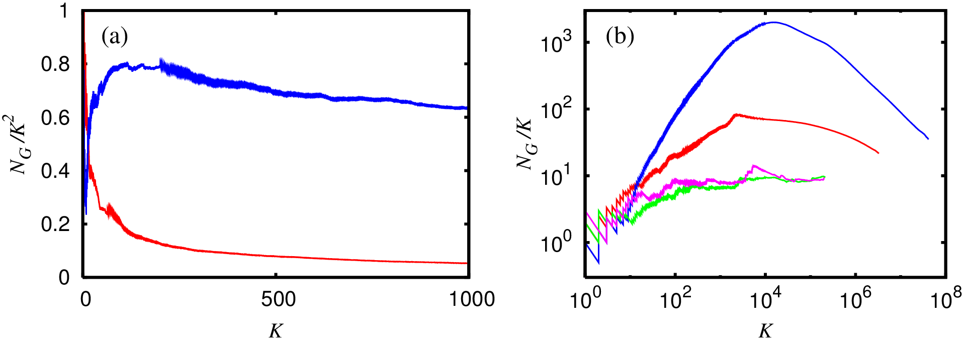
The decay exponent of the PageRank is for Twitter $\beta=0.540$ (for $1\leq K\leq 10^{6}$), which indicates a precursor of a delocalization transition as compared to Wikipedia ($\beta=0.767$) or WWW ($\beta\approx 0.9$), caused by the strong interconnectivity Frahm and Shepelyansky (2012b). The Twitter network is also characterized by a large value of PageRank-CheiRank correlator $\kappa=112.6$ that is by a factor $30-60$ larger than this value for Wikipedia and University networks. Such a larger value of $\kappa$ results from certain individual large values $\kappa_{i}=NP(K(i))P^{*}(K^{*}(i))\sim 1$. It is argued that this is related to a very strong inter-connectivity between top K PageRank users of the Twitter network Frahm and Shepelyansky (2012b).

Figure 33: (Color online) Spectrum of the Twitter matrix $S$ (a) and (c), and $S^{*}$ (b) and (d). Panels (a) and (b) show subspace eigenvalues (blue/black dots) and core space eigenvalues (red/gray dots) in $\lambda$-plane (green/gray curve shows unit circle); there are 17504 (66316) invariant subspaces, with maximal dimension 44 (2959) and the sum of all subspace dimensions is $N_{s}=40307$ (180414). The core space eigenvalues are obtained from the Arnoldi method applied to the core space subblock $S_{cc}$ of $S$ with Arnoldi dimension $n_{A}=640$. Panels (c) and (d) show the fraction $j/N$ of eigenvalues with $|\lambda|>|\lambda_{j}|$ for the core space eigenvalues (red/gray bottom curve) and all eigenvalues (blue/black top curve) from raw data ((a) and (b) respectively). The number of eigenvalues with $|\lambda_{j}|=1$ is 34135 (129185) of which 17505 (66357) are at $\lambda_{j}=1$; this number is (slightly) larger than the number of invariant subspaces which have each at least one unit eigenvalue. Note that in panels (c) and (d) the number of eigenvalues with $|\lambda_{j}|=1$ is artificially reduced to 200 in order to have a better scale on the vertical axis. The correct numbers of those eigenvalues correspond to $j/N=8.195\times 10^{-4}$ (c) and $3.102\times 10^{-3}$ (d) which are strongly outside the vertical panel scale. After Frahm and Shepelyansky (2012b).

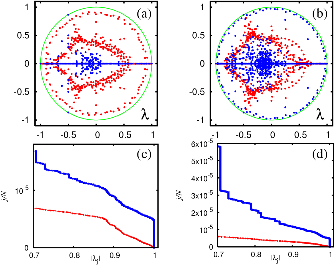
The spectra of matrices $S$ and $S^{*}$ are obtained with the help of the Arnoldi method for a relatively modest Arnoldi dimension due to a very large matrix size. The largest $n_{A}$ modulus eigenvalues $|\lambda|$ are shown in Fig. 33. The invariant subspaces (see Sec. III.3) for the Twitter network cover about $N_{s}=4\times 10^{4}$ ($1.8\times 10^{5}$) nodes for $S$ ($S^{*}$) leading to $1.7\times 10^{4}$ ($6.6\times 10^{4}$) eigenvalues with $\lambda_{j}=1$ or even $3.4\times 10^{4}$ ($1.3\times 10^{5}$) eigenvalues with $|\lambda_{j}|=1$. However, for Twitter the fraction of subspace nodes $g_{1}=N_{s}/N\approx 10^{-3}$ is smaller than the fraction $g_{1}\approx 0.2$ for the university networks of Cambridge or Oxford (with $N\approx 2\times 10^{5}$) since the size of the whole Twitter network is significantly larger. The complex spectra of $S$ and $S^{*}$ also show the cross and triple-star structures, as in the cases of Cambridge and Oxford 2006 (see Fig. 17), even though for the Twitter network they are significantly less pronounced.

X.2 Poisson statistics of PageRank probabilities

From a physical viewpoint one can conjecture that the PageRank probabilities are described by a steady-state quantum Gibbs distribution over certain quantum levels with energies $E_{i}$ by the identification $P(i)=\exp(-E_{i}/T)/Z$ with $Z=\sum_{i}\exp(-E_{i}/T)$ Frahm and Shepelyansky (2014a). In some sense this conjecture assumes that the operator matrix $G$ can be represented as a sum of two operators $G_{H}$ and $G_{NH}$ where $G_{H}$ describes a Hermitian system while $G_{NH}$ represents a non-Hermitian operator which creates a system thermalization at a certain effective temperature $T$ with the quantum Gibbs distribution over energy levels $E_{i}$ of the operator $G_{H}$.

Figure 34: (Color online) Panel (a) shows the dependence of certain top PageRank levels $E_{i}=-\ln(P_{i})$ on the damping factor $\alpha$ for Twitter network. Data points on curves with one color corresponds to the same node $i$; about 150 levels are shown close to the minimal energy $E\approx 7.5$. Panel (b) represents the histogram of unfolded level spacing statistics for Twitter at $10<K\leq 10^{4}$. The Poisson distribution $p_{\rm Pois}(s)=\exp(-s)$ and the Wigner surmise $p_{\rm Wig}(s)=\frac{\pi}{2}\,s\,\exp(-\frac{\pi}{4}\,s^{2})$ are also shown for comparison. After Frahm and Shepelyansky (2014a).

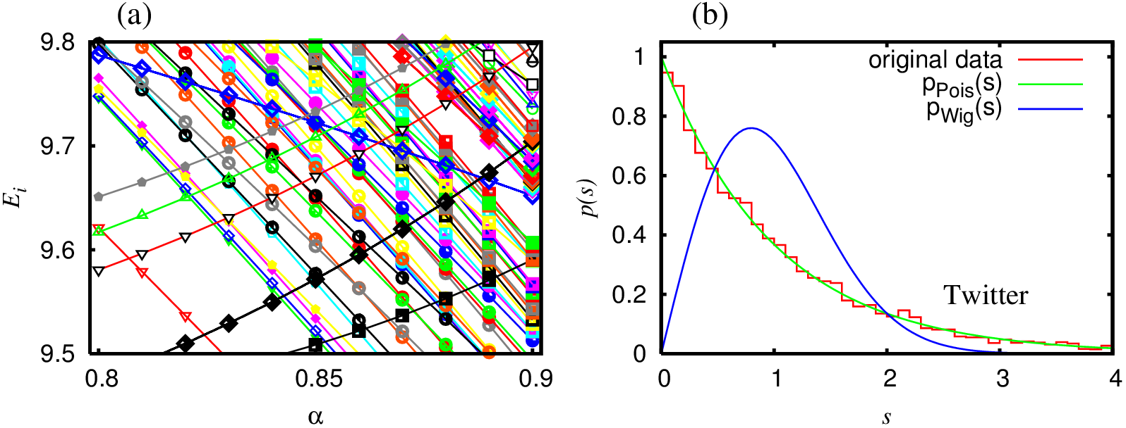
The identification of PageRank with an energy spectrum allows to study the corresponding level statistics which represents a well known concept in the framework of Random Matrix Theory Mehta (2004); Guhr et al. (1998). The most direct characteristic is the probability distribution $p(s)$ of unfolded level spacings $s$. Here $s=(E_{i+1}-E_{i})/\Delta E$ is a spacing between nearest levels measured in the units of average local energy spacing $\Delta E$. The unfolding procedure Mehta (2004); Guhr et al. (1998) requires the smoothed dependence of $E_{i}$ on the index $K$ which is obtained from a polynomial fit of $E_{i}\sim\ln(P_{i})$ with $\ln(K)$ as argument Frahm and Shepelyansky (2014a).

The statistical properties of fluctuations of levels have been extensively studied in the fields of RMT Mehta (2004), quantum chaos Haake (2010) and disordered solid state systems Evers and Mirlin (2008). It is known that integrable quantum systems have $p(s)$ well described by the Poisson distribution $p_{\rm Pois}(s)=\exp(-s)$. In contrast the quantum systems, which are chaotic in the classical limit (e.g. Sinai billiard), have $p(s)$ given by the RMT being close to the Wigner surmise $p_{\rm Wig}(s)=\frac{\pi}{2}\,s\,\exp(-\frac{\pi}{4}\,s^{2})$ Bohigas et al. (1984). Also the Anderson localized phase is characterized by $p_{\rm Pois}(s)$ while in the delocalized regime one has $p_{\rm Wig}(s)$ Evers and Mirlin (2008).

The results for the Twitter PageRank level statistics Frahm and Shepelyansky (2014a) are shown in Fig. 34. We find that $p(s)$ is well described by the Poisson distribution. Furthermore, the evolution of energy levels $E_{i}$ with the variation of the damping factor $\alpha$ shows many level crossings which are typical for Poisson statistics. We may note that here each level has its own index so that it is rather easy to see if there is a real or avoided level crossing.

The validity of the Poisson statistics for PageRank probabilities is confirmed also for the networks of Wikipedia editions in English, French and German from Fig. 24 Frahm and Shepelyansky (2014a). We argue that due to absence of level repulsion the PageRank order of nearby nodes can be easily interchanged. The obtained Poisson law implies that the nearby PageRank probabilities fluctuate as random independent variables.

XI Google matrix analysis of world trade

During the last decades the trade between countries has been developed in an extraordinary way. Usually countries are ranked in the world trade network (WTN) taking into account their exports and imports measured in USD CIA (2009). However, the use of these quantities, which are local in the sense that countries know their total imports and exports, could hide the information of the centrality role that a country plays in this complex network. In this section we present the two-dimensional Google matrix analysis of the WTN introduced in Ermann and Shepelyansky (2011b). Some previous studies of global network characteristics were considered in Garlaschelli and Loffredo (2005); Serrano et al. (2007), degree centrality measures were analyzed in De Benedictis and Tajoli (2011) and a time evolution of network global characteristics was studied in He and Deem (2010). Topological and clustering properties of multiplex network of various commodities were discussed in Barigozzi et al. (2010), and an ecological ranking based on the nestedness of countries and products was presented in Ermann and Shepelyansky (2013a).

The money exchange between countries defines a directed network. Therefore Google matrix analysis can be introduced in a natural way. PageRank and CheiRank algorithms can be easily applied to this network with a straightforward correspondence with imports and exports. Two-dimensional ranking, introduced in Sec. IV, gives an illustrative representation of global importance of countries in the WTN. The important element of Google ranking of WTN is its democratic treatment of all world countries, independently of their richness, that follows the main principle of the United Nations (UN).

XI.1 Democratic ranking of countries

The WTN is a directed network that can be constructed considering countries as nodes and money exchange as links. We follow the definition of the WTN of Ermann and Shepelyansky (2011b) where trade information comes from UN COMTRADE (2011). These data include all trades between countries for different products (using Standard International Trade Classification of goods, SITC1) from 1962 to 2009.

All useful information of the WTN is expressed via the money matrix $M$, which definition, in terms of its matrix elements $M_{ij}$, is defined as the money transfer (in USD) from country $j$ to country $i$ in a given year. This definition can be applied to a given specific product or to all commodities, which represent the sum over all products.

In contrast to the binary adjacency matrix $A_{ij}$ of WWW (as the ones analyzed in SVIII and SX for example) $M$ has weighted elements. This corresponds to a case when there are in principle multiple number of links from $j$ to $i$ and this number is proportional to USD amount transfer. Such a situation appears in Sec. VI for Ulam networks and Sec. VII for Linux PCN with a main difference that for the WTN case there is a very large variation of mass matrix elements $M_{ij}$, related to the fact that there is a very strong variation of richness of various countries.

Google matrices $G$ and $G^{*}$ are constructed according to the usual rules and relation (1) with $M_{ij}$ and its transposed: $S_{ij}=M_{ij}/m_{j}$ and $S_{ij}=M_{ji}/m^{*}_{j}$ where $S_{ij}=1/N$ and $S^{*}_{ij}=1/N$, if for a given $j$ all elements $M_{ij}=0$ and $M_{ji}=0$ respectively. Here $m_{j}=\sum_{i}M_{ij}$ and $m^{*}_{j}=\sum_{i}M_{ji}$ are the total export and import mass for country $j$. Thus the sum in each column of $G$ or $G^{*}$ is equal to unity. In this way Google matrices $G$ and $G^{*}$ of WTN allow to treat all countries on equal grounds independently of the fact if a given country is rich or poor. This kind of analysis treats in a democratic way all world countries in consonance with the standards of the UN.

The probability distributions of ordered PageRank $P(K)$ and CheiRank $P^{*}(K^{*})$ depend on their indexes in a rather similar way with a power law decay given by $\beta$. For the fit of top 100 countries and all commodities the average exponent value is close to $\beta=1$ corresponding to the Zipf law Zipf (1949).

Figure 35: (Color online) Country positions in PageRank-CheiRank plane $(K,K^{*})$ for world trade in various commodities in 2008. Each country is shown by circle with its own flag (for a better visibility the circle center is slightly displaced from its integer position $(K,K^{*})$ along direction angle $\pi/4$). The panels show the ranking for trade in the following commodities: all commodities (a) and (b); and crude petroleum (c) and (d). Panels (a) and (c) show a global scale with all 227 countries, while (b) and (d) give a zoom in the region of $40\times 40$ top ranks. After Ermann and Shepelyansky (2011b).

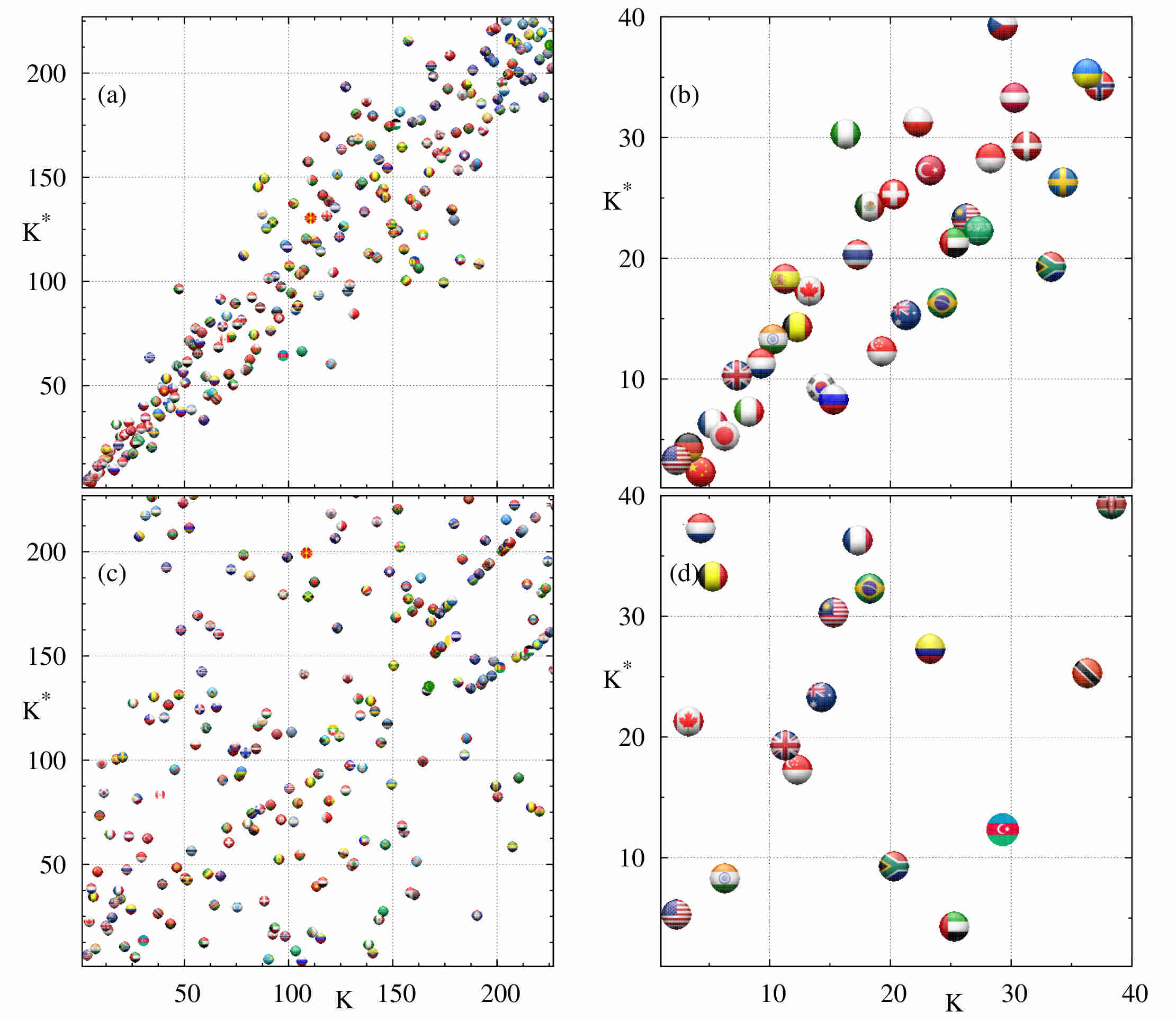
The distribution of countries on PageRank-CheiRank plane for trade in all commodities in year 2008 is shown in panels (a) and (b) of Fig. 35 at $\alpha=0.5$. Even if the Google matrix approach is based on a democratic ranking of international trade, being independent of total amount of export-import and PIB for a given country, the top ranks $K$ and $K^{*}$ belong to the group of industrially developed countries. This means that these countries have efficient trade networks with optimally distributed trade flows. Another striking feature of global distribution is that it is concentrated along the main diagonal $K=K^{*}$. This feature is not present in other networks studied before. The origin of this density concentration is related to a simple economy reason: for each country the total import is approximately equal to export since each country should keep in average an economic balance. This balance does not imply a symmetric money matrix, used in gravity model of trade (see e.g. Krugman et al. (2011); De Benedictis and Tajoli (2011)), as can be seen in the significant broadening of distribution of Fig. 35 (especially at middle values of $K\sim 100$).

For a given country its trade is doing well if its $K^{*}<K$ so that the country exports more than it imports. The opposite relation $K^{*}>K$ corresponds to a bad trade situation (e.g. Greece being significantly above the diagonal). We also can say that local minima in the curve of $(K^{*}-K)\;vs.\;K$ correspond to a successful trade while maxima mark bad traders. In 2008 most successful were China, R of Korea, Russia, Singapore, Brazil, South Africa, Venezuela (in order of $K$ for $K\leq 50$) while among bad traders we note UK, Spain, Nigeria, Poland, Czech Rep, Greece, Sudan with especially strong export drop for two last cases.

A comparison between local and global rankings of countries for both imports and exports gives a new tool to analyze countries economy. For example, in 2008 the most significant differences between CheiRank and the rank given by total exports are for Canada and Mexico with corresponding money export ranks $\tilde{K}^{*}=11$ and $13$ and with $K^{*}=16$ and $K^{*}=23$ respectively. These variations can be explained in the context that the export of these two countries is too strongly oriented on USA. In contrast Singapore moves up from $\tilde{K}^{*}=15$ export position to $K^{*}=11$ that shows the stability and broadness of its export trade, a similar situation appears for India moving up from $\tilde{K}^{*}=19$ to $K^{*}=12$ (see Ermann and Shepelyansky (2011b) for more detailed analysis).

XI.2 Ranking of countries by trade in products

If we focus on the two-dimensional distribution of countries in a specific product we obtain a very different information. The symmetry approximately visible for all commodities is absolutely absent: the points are scattered practically over the whole square $N\times N$ (see Fig. 35). The reason of such a strong scattering is clear: e.g. for crude petroleum some countries export this product while other countries import it. Even if there is some flow from exporters to exporters it remains relatively low. This makes the Google matrix to be very asymmetric. Indeed, the asymmetry of trade flow is well visible in panels (c) and (d) of Fig. 35.

Figure 36: (Color online) Spindle distribution for WTN of all commodities for all countries in the period 1962 - 2009 shown in the plane of $((K^{*}-K)/N,(K^{*}+K)/N)$ (coarse-graining inside each of $76\times 152$ cells); data from the UN COMTRADE database. After Ermann and Shepelyansky (2011b).

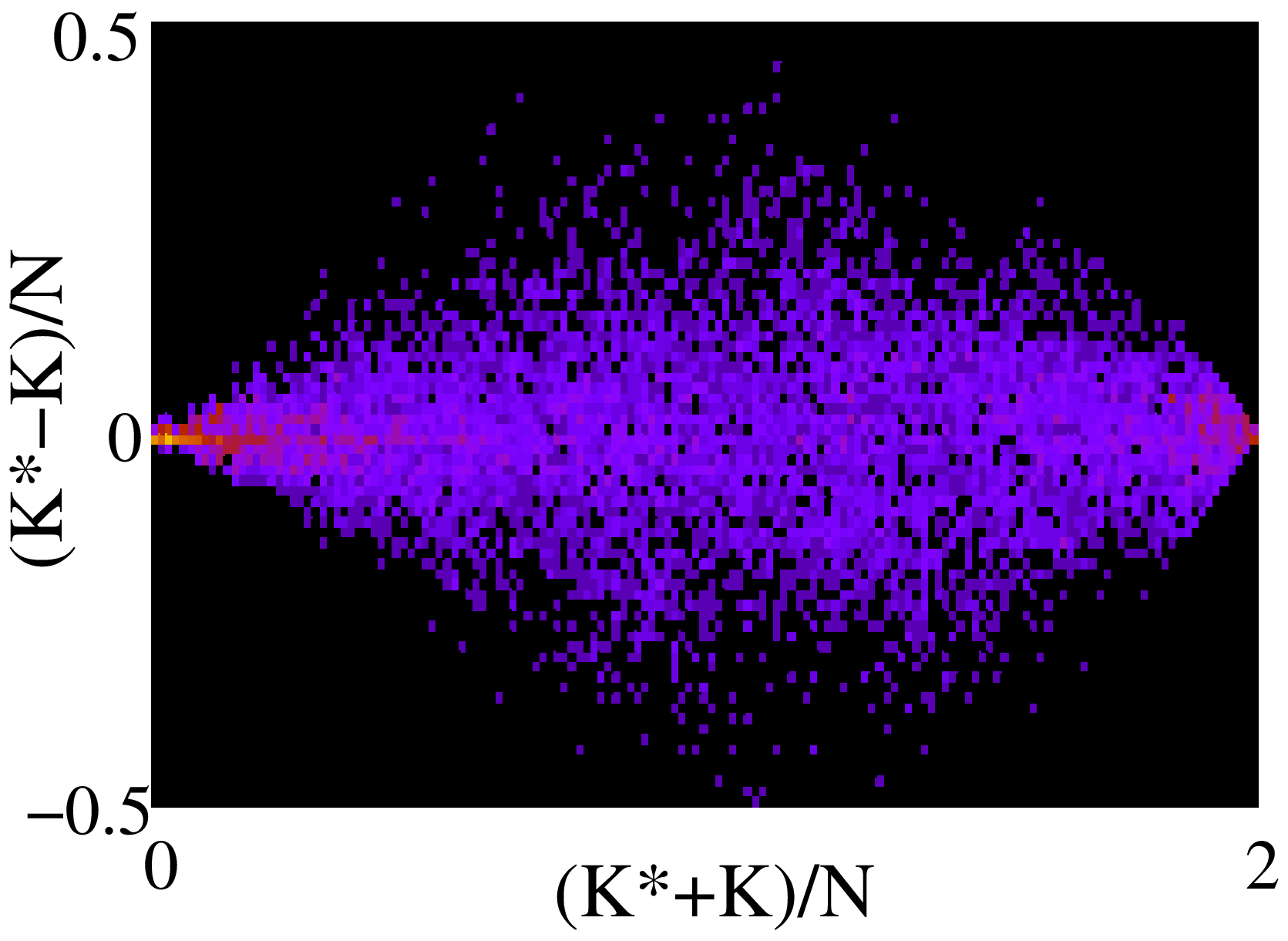
The same comparison of global and local rankings done before for all commodities can be applied to specific products obtaining even more strong differences. For example for crude petroleum Russia moves up from $\tilde{K}^{*}=2$ export position to $K^{*}=1$ showing that its trade network in this product is better and broader than the one of Saudi Arabia which is at the first export position $\tilde{K}^{*}=1$ in money volume. Iran moves in opposite direction from $\tilde{K}^{*}=5$ money position down to $K^{*}=14$ showing that its trade network is restricted to a small number of nearby countries. A significant improvement of ranking takes place for Kazakhstan moving up from $\tilde{K}^{*}=12$ to $K^{*}=2$. The direct analysis shows that this happens due to an unusual fact that Kazakhstan is practically the only country which sells crude petroleum to the CheiRank leader in this product Russia. This puts Kazakhstan on the second position. It is clear that such direction of trade is more of political or geographical origin and is not based on economic reasons.

The same detailed analysis can be applied to all specific products given by SITC1. For example for trade of cars France goes up from $\tilde{K}^{*}=7$ position in exports to $K^{*}=3$ due to its broad export network.

XI.3 Ranking time evolution and crises

The WTN has evolved during the period 1962 - 2009. The number of countries is increased by 38%, while the number of links per country for all commodities is increased in total by 140% with a significant increase from 50% to 140% during the period 1993 - 2009 corresponding to economy globalization. At the same time for a specific commodity the average number of links per country remains on a level of 3-5 links being by a factor 30 smaller compared to all commodities trade. During the whole period the total amount $M_{T}$ of trade in USD shows an average exponential growth by 2 orders of magnitude.

A statistical density distribution of countries in the plane $(K^{*}-K,K^{*}+K)$ in the period 1962 - 2009 for all commodities is shown in Fig. 36. The distribution has a form of spindle with maximum density at the vertical axis $K^{*}-K=0$. We remind that good exporters are on the lower side of this axis at $K^{*}-K<0$, while the good importers (bad exporters) are on the upper side at $K^{*}-K>0$.

Figure 37: (Color online) Time evolution of CheiRank and PageRank indexes $K$, $K^{*}$ for some selected countries for all commodities. The countries shown panels (a) and (b) are: Japan (jp-black), France (fr-red), Fed R of Germany and Germany (de - both in blue), Great Britain (gb - green), USA (us - orange) [curves from top to bottom in 1962 in (a)]. The countries shown panels (c) and (d) are: Argentina (ar - violet), India (in - dark green), China (cn - cyan), USSR and Russian Fed (ru - both in gray) [curves from top to bottom in 1975 in (c)]. After Ermann and Shepelyansky (2011b).

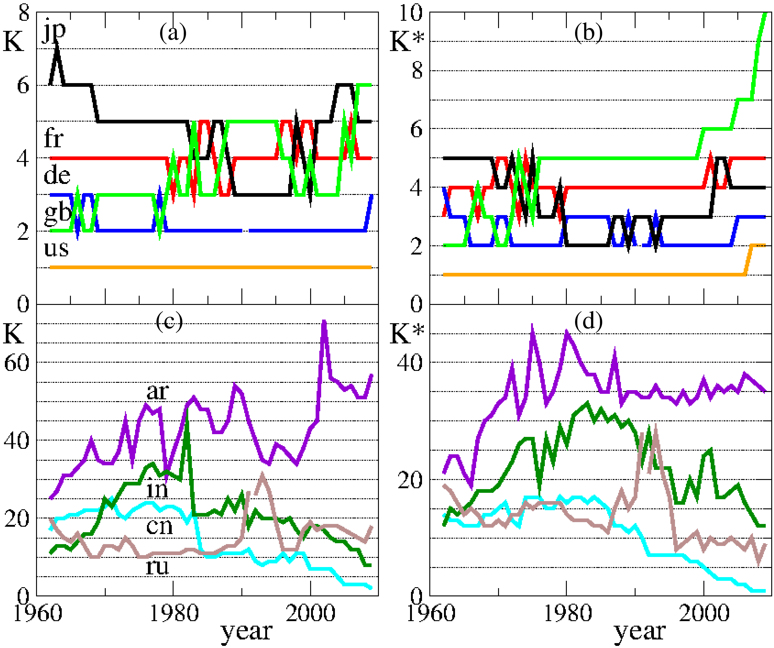
The evolution of the ranking of countries for all commodities reflects their economical changes. The countries that occupy top positions tend to move very little in their ranks and can be associated to a solid phase. On the other hand, the countries in the middle region of $K^{*}+K$ have a gas like phase with strong rank fluctuations.

Examples of ranking evolution $K$ and $K^{*}$ for Japan, France, Fed R of Germany and Germany, Great Britain, USA, and for Argentina, India, China, USSR and Russian Fed are shown in Fig. 37. It is interesting to note that sharp increases in $K$ mark crises in 1991, 1998 for Russia and in 2001 for Argentina (import is reduced in period of crises). It is also visible that in recent years the solid phase is perturbed by entrance of new countries like China and India. Other regional or global crisis could be highlighted due to the big fluctuations in the evolution of ranks. For example, in the range $81\leq K+K^{*}\leq 120$, during the period of 1992 - 1998 some financial crises as Black Wednesday, Mexico crisis, Asian crisis and Russian crisis are appreciated with this ranking evolution.

XI.4 Ecological ranking of world trade

Interesting parallels between multiproduct world trade and interactions between species in ecological systems has been traced in Ermann and Shepelyansky (2013a). This approach is based on analysis of strength of transitions forming the Google matrix for the multiproduct world trade network.

Ecological systems are characterized by high complexity and biodiversity May (2001) linked to nonlinear dynamics and chaos emerging in the process of their evolution Lichtenberg and Lieberman (1992). The interactions between species form a complex network whose properties can be analyzed by the modern methods of scale-free networks. The analysis of their properties uses a concept of mutualistic networks and provides a detailed understanding of their features being linked to a high nestedness of these networks Burgos et al. (2007); Bastolla et al. (2009); Saverda et al. (2011); Burgos et al. (2008). Using the UN COMTRADE database we show that a similar ecological analysis gives a valuable description of the world trade: countries and trade products are analogous to plants and pollinators, and the whole trade network is characterized by a high nestedness typical for ecological networks.

An important feature of ecological networks is that they are highly structured, being very different from randomly interacting species Bascompte et al. (2003). Recently is has been shown that the mutualistic networks between plants and their pollinators Bascompte et al. (2003); Vázquez and Aizen (2004); Memmott et al. (2004); Olesen et al. (2007); Rezende et al. (2007) are characterized by high nestedness which minimizes competition and increases biodiversity Burgos et al. (2007); Bastolla et al. (2009); Saverda et al. (2011); Burgos et al. (2008).

Figure 38: (Color online) Nestedness matrices for the plant-animal mutualistic networks on top panels, and for the WTN of countries-products on middle and bottom panels. Panels (a) and (b) represent data of ARR1 and WES networks from Rezende et al. (2007). The WTN matrices are computed with the threshold $\mu=10^{-3}$ and corresponding $\varphi\approx 0.2$ for years 2008 (c,d) and 1968 (e,f) and 2008 for import (c,e) and export (d,f) panels. Red/gray and blue/black represent unit and zero elements respectively; only lines and columns with nonzero elements are shown. The order of plants-animals, countries-products is given by the nestedness algorithm Rodríguez-Gironés et al. (2006), the perfect nestedness is shown by green/gray curves for the corresponding values of $\varphi$. After Ermann and Shepelyansky (2013a).

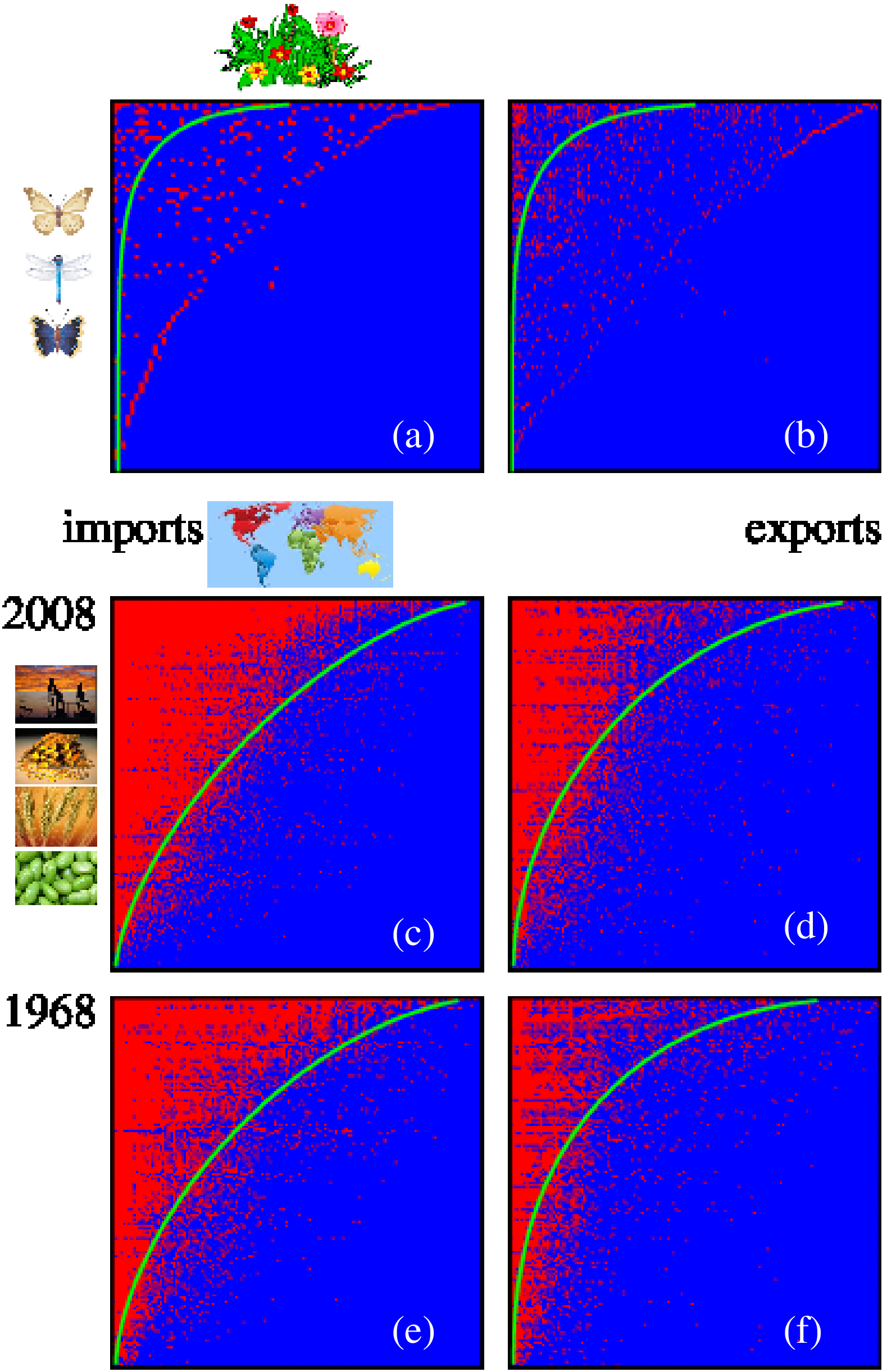
The mutualistic WTN is constructed on the basis of the UN COMTRADE database from the matrix of trade transactions $M^{p}_{c^{\prime},c}$ expressed in USD for a given product (commodity) $p$ from country $c$ to country $c^{\prime}$ in a given year (from 1962 to 2009). For product classification we use 3–digits SITC Rev.1 discussed above with the number of products $N_{p}=182$. All these products are described in UN COMTRADE (2011) in the commodity code document SITC Rev1. The number of countries varies between $N_{c}=164$ in 1962 and $N_{c}=227$ in 2009. The import and export trade matrices are defined as $M^{(i)}_{p,c}=\sum_{c^{\prime}=1}^{N_{c}}M^{p}_{c,c^{\prime}}$ and $M^{(e)}_{p,c}=\sum_{c^{\prime}=1}^{N_{c}}M^{p}_{c^{\prime},c}$ respectively. We use the dimensionless matrix elements $m^{(i)}=M^{(i)}/M_{max}$ and $m^{(e)}=M^{(e)}/M_{max}$ where for a given year $M_{max}=max\{max[M^{(i)}_{p,c}],max[M^{(e)}_{p,c}]\}$. The distribution of matrix elements $m^{(i)}$, $m^{(e)}$ in the plane of indexes $p$ and $c$, ordered by the total amount of import/export in a decreasing order, are shown and discussed in Ermann and Shepelyansky (2013a). In global, the distributions of $m^{(i)}$, $m^{(e)}$ remain stable in time especially in a view of 100 times growth of the total trade volume during the period 1962-2009. The fluctuations of $m^{(e)}$ are larger compared to $m^{(i)}$ case since certain products, e.g. petroleum, are exported by only a few countries while it is imported by almost all countries.

To use the methods of ecological analysis we construct the mutualistic network matrix for import $Q^{(i)}$ and export $Q^{(e)}$ whose matrix elements take binary value $1$ or $0$ if corresponding elements $m^{(i)}$ and $m^{(e)}$ are respectively larger or smaller than a certain trade threshold value $\mu$. The fraction $\varphi$ of nonzero matrix elements varies smoothly in the range $10^{-6}\leq\mu\leq 10^{-2}$ and the further analysis is not really sensitive to the actual $\mu$ value inside this broad range.

Figure 39: (Color online) Top 20 EcoloRank countries as a function of years for the WTN import (a) and export (b) panels. The ranking is given by the nestedness algorithm for the trade threshold $\mu=10^{-3}$; each country is represented by its corresponding flag. As an example, dashed lines show time evolution of the following countries: USA, UK, Japan, China, Spain. After Ermann and Shepelyansky (2013a).

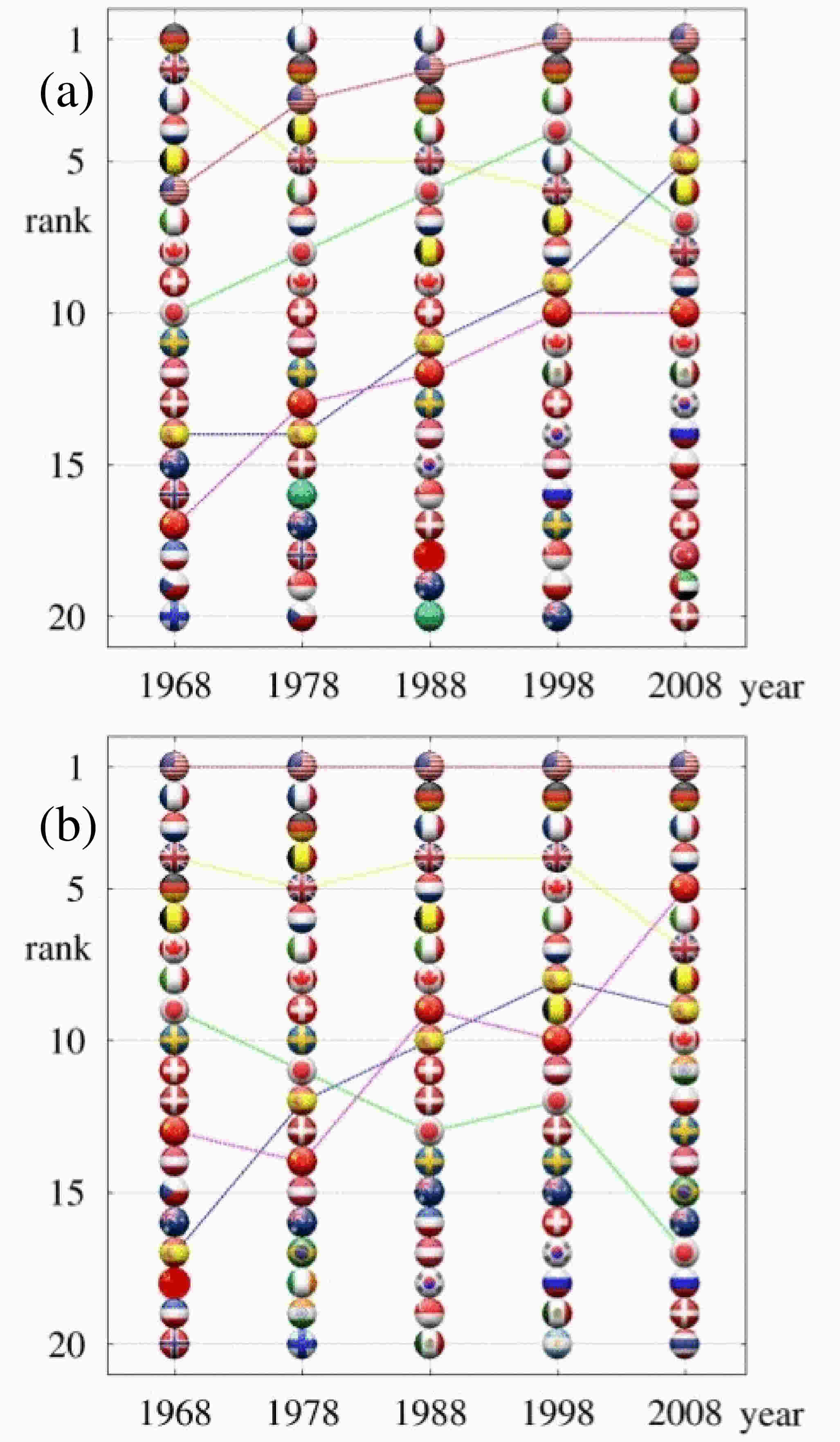
In contrast to ecological systems Bastolla et al. (2009) the world trade is described by a directed network and hence we characterize the system by two mutualistic matrices $Q^{(i)}$ and $Q^{(e)}$ corresponding to import and export. Using the standard nestedness BINMATNEST algorithm Rodríguez-Gironés et al. (2006) we determine the nestedness parameter $\eta$ of the WTN and the related nestedness temperature $T=100(1-\eta)$. The algorithm reorders lines and columns of a mutualistic matrix concentrating nonzero elements as much as possible in the top left corner and thus providing information about the role of immigration and extinction in an ecological system. A high level of nestedness and ordering can be reached only for systems with low $T$. It is argued that the nested architecture of real mutualistic networks increases their biodiversity.

Figure 40: (Color online) Top 20 countries as a function of years ranked by the total monetary trade volume of the WTN in import (a) and export (b) panels respectively; each country is represented by its corresponding flag. Dashed lines show time evolution of the same countries as in Fig. 39. After Ermann and Shepelyansky (2013a).

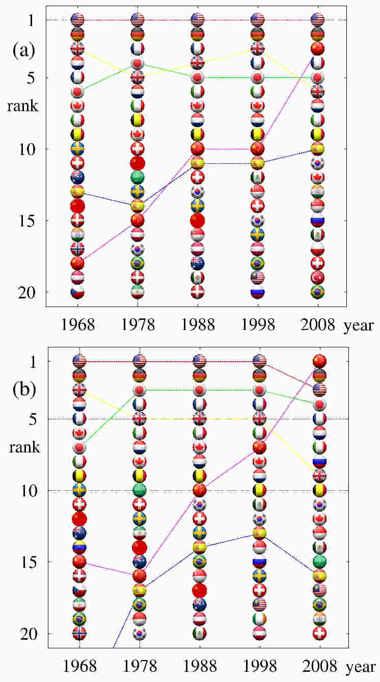
The nestedness matrices generated by the BINMATNEST algorithm Rodríguez-Gironés et al. (2006) are shown in Fig. 38 for ecology networks ARR1 ($N_{pl}=84$, $N_{anim}=101$, $\varphi=0.043$, $T=2.4$) and WES ($N_{pl}=207$, $N_{anim}=110$, $\varphi=0.049$, $T=3.2$) from Rezende et al. (2007). Using the same algorithm we generate the nestedness matrices of WTN using the mutualistic matrices for import $Q^{(i)}$ and export $Q^{(i)}$ for the WTN in years 1968 and 2008 using a fixed typical threshold $\mu=10^{-3}$ (see Fig. 38). As for ecological systems, for the WTN data we also obtain rather small nestedness temperature ($T\approx 6/8$ for import/export in 1968 and $T\approx 4/8$ in 2008 respectively). These values are by a factor 9/4 of times smaller than the corresponding $T$ values for import/export from random generated networks with the corresponding values of $\varphi$.

Figure 41: (Color online) Top 10 ranks of trade products as a function of years for the WTN. Panel (a): ranking of products by monetary trade volume. Panels (b), (c): ranking is given by the nestedness algorithm for import (b) and export (c) with the trade threshold $\mu=10^{-3}$. Each product is shown by its own symbol with short name written at years 1968, 2008; symbol color marks 1st SITC digit; SITC codes of products and their names are given in UN COMTRADE (2011) and Table 2 in Ermann and Shepelyansky (2013a). After Ermann and Shepelyansky (2013a).

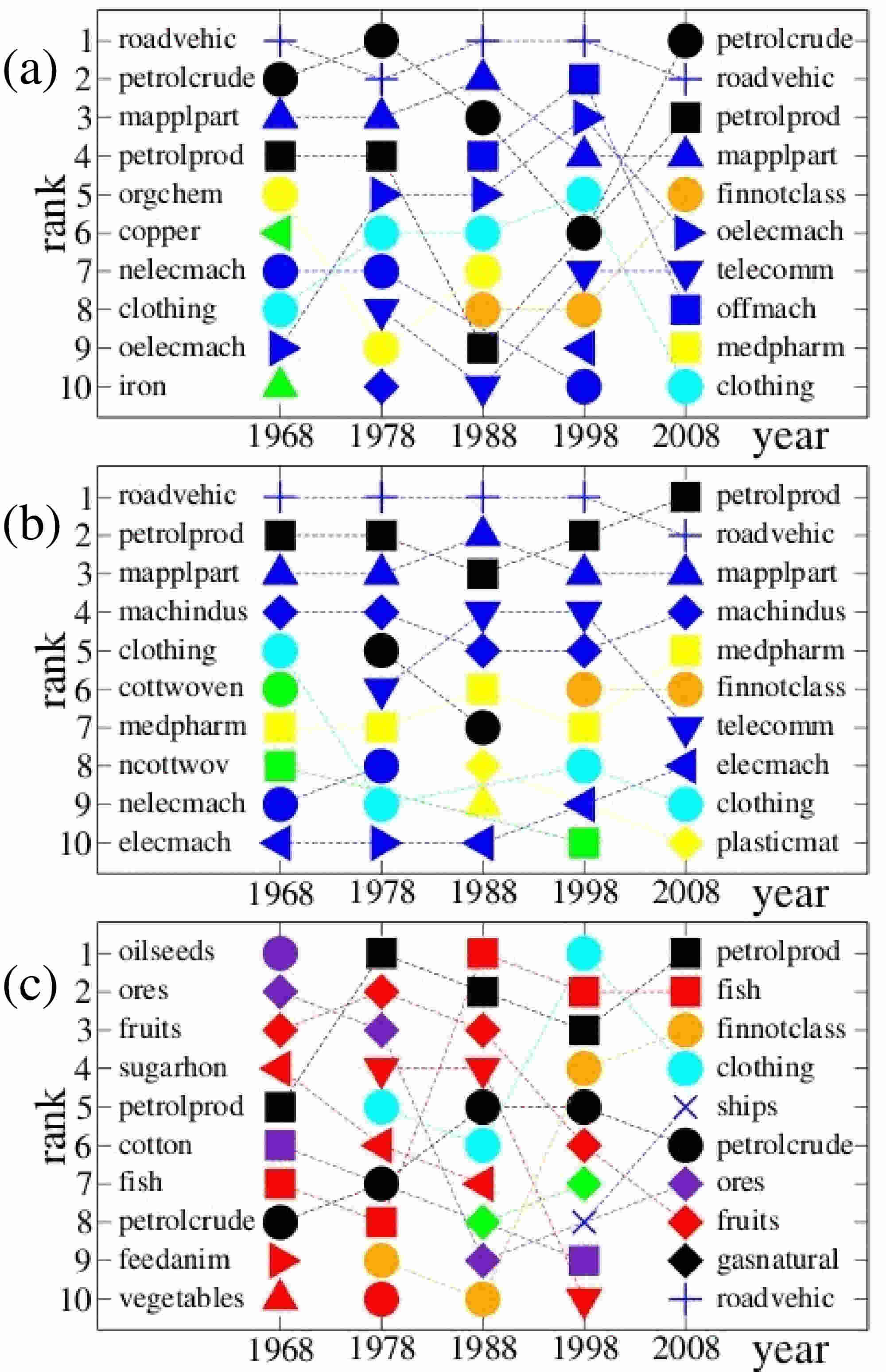
The small value of nestedness temperature obtained for the WTN confirms the validity of the ecological analysis of WTN structure: trade products play the role of pollinators which produce exchange between world countries, which play the role of plants. Like in ecology the WTN evolves to the state with very low nestedness temperature that satisfies the ecological concept of system stability appearing as a result of high network nestedness Bastolla et al. (2009).

The nestedness algorithm creates effective ecological ranking (EcoloRanking) of all UN countries. The evolution of 20 top ranks throughout the years is shown in Fig. 39 for import and export. This ranking is quite different from the more commonly applied ranking of countries by their total import/export monetary trade volume CIA (2009) (see corresponding data in Fig. 40) or the democratic ranking of WTN based on the Google matrix analysis discussed above. Indeed, in 2008 China is at the top rank for total export volume but it is only at 5th position in EcoloRank (see Fig. 39, Fig. 40). In a similar way Japan moves down from 4th to 17th position while USA raises up from 3rd to 1st rank.

The same nestedness algorithm generates not only the ranking of countries but also the ranking of trade products for import and export which is presented in Fig. 41. For comparison we also show there the standard ranking of products by their trade volume. In Fig. 41 the color of symbol marks the 1st SITC digit described in figure, UN COMTRADE (2011) and Table 2 in Ermann and Shepelyansky (2013a).

The origin of such a difference between EcoloRanking and trade volume ranking of countries is related to the main idea of mutualistic ranking in ecological systems: the nestedness ordering stresses the importance of mutualistic pollinators (products for WTN) which generate links and exchange between plants (countries for WTN). In this way generic products, which participate in the trade between many countries, become of primary importance even if their trade volume is not at the top lines of import or export. In fact such mutualistic products glue the skeleton of the world trade while the nestedness concept allows to rank them in order of their importance. The time evolution of this EcoloRanking of products of WTN is shown in Fig. 41 for import/export in comparison with the product ranking by the monetary trade volume (since the trade matrix is diagonal in product index the ranking of products in the latter case is the same for import/export). The top and middle panels have dominate colors corresponding to machinery (SITC Rev. 1 code 7; blue) and mineral fuels (3; black) with a moderate contribution of chemicals (5; yellow) and manufactured articles (8; cyan) and a small fraction of goods classified by material (6; green). Even if the global structure of product ranking by trade volume has certain similarities with import EcoloRanking there are also important new elements. Indeed, in 2008 the mutualistic significance of petroleum products (code 332), machindus (machines for special industries code 718) and medpharm (medical-pharmaceutic products code 541) is much higher compared to their volume ranking, while petroleum crude (code 331) and office machines (code 714) have smaller mutualistic significance compared to their volume ranking.

The new element of EcoloRanking is that it differentiates between import and export products while for trade volume they are ranked in the same way. Indeed, the dominant colors for export (Fig. 41 bottom panel) correspond to food (SITC Rev. 1 code 0; red) with contribution of black (present in import) and crude materials (code 2; violet); followed by cyan (present in import) and more pronounced presence of finnotclass (commodities/transactions not classified code 9; brown). EcoloRanking of export shows a clear decrease tendency of dominance of SITC codes 0 and 2 with time and increase of importance of codes 3,7. It is interesting to note that the code 332 of petroleum products is vary vulnerable in volume ranking due to significant variations of petroleum prices but in EcoloRanking this product keeps the stable top positions in all years showing its mutualistic structural importance for the world trade. EcoloRanking of export shows also importance of fish (code 031), clothing (code 841) and fruits (code 051) which are placed on higher positions compared to their volume ranking. At the same time roadvehic (code 732), which are at top volume ranking, have relatively low ranking in export since only a few countries dominate the production of road vehicles.

It is interesting to note that in Fig. 41 petroleum crude is at the top of trade volume ranking e.g. in 2008 (top panel) but it is absent in import EcoloRanking (middle panel) and it is only on 6th position in export EcoloRanking (bottom panel). A similar feature is visible for years 1968, 1978. On a first glance this looks surprising but in fact for mutualistic EcoloRanking it is important that a given product is imported from top EcoloRank countries: this is definitely not the case for petroleum crude which practically is not produced inside top 10 import EcoloRank countries (the only exception is USA, which however also does not export much). Due to that reason this product has low mutualistic significance.

The mutualistic concept of product importance is at the origin of significant difference of EcoloRanking of countries compared to the usual trade volume ranking (see Fig. 39, Fig. 40). Indeed, in the latter case China and Japan are at the dominant positions but their trade is concentrated in specific products which mutualistic role is relatively low. In contrast USA, Germany and France keep top three EcoloRank positions during almost 40 years clearly demonstrating their mutualistic power and importance for the world trade.

Thus our results show the universal features of ecologic ranking of complex networks with promising future applications to trade, finance and other areas.

XI.5 Remarks on world trade and banking networks

The new approach to the world trade, based on the Google matrix analysis, gives a democratic type of ranking being independent of the trade amount of a given country. In this way rich and poor countries are treated on equal democratic grounds. In a certain sense PageRank probability for a given country is proportional to its rescaled import flows while CheiRank is proportional to its rescaled export flows inside of the WTN.

The global characteristics of the world trade are analyzed on the basis of this new type of ranking. Even if all countries are treated now on equal democratic grounds still we find at the top rank the group of industrially developed countries approximately corresponding to G-20 and recover 74% of countries listed in G-20. The Google matrix analysis demonstrates an existence of two solid state domains of rich and poor countries which remain stable during the years of consideration. Other countries correspond to a gas phase with ranking strongly fluctuating in time. We propose a simple random matrix model which well describes the statistical properties of rank distribution for the WTN Ermann and Shepelyansky (2011b).

The comparison between usual ImportRank–ExportRank (see e.g. CIA (2009)) and our PageRank–CheiRank approach shows that the later highlights the trade flows in a new useful manner which is complementary to the usual analysis. The important difference between these two approaches is due to the fact that ImportRank–ExportRank method takes into account only global amount of money exchange between a country and the rest of the world while PageRank–CheiRank approach takes into account all links and money flows between all countries.

The future developments should consider a matrix with all countries and all products which size becomes significantly larger ($N\sim 220\times 10^{4}\sim 2\times 10^{6}$) comparing to a modest size $N\approx 227$ considered here. However, some new problems of this multiplex network analysis should be resolved combining a democracy in countries with volume importance of products which role is not democratic. It is quite possible that such an improved analysis will generate an asymmetric ranking of products in contrast to their symmetric ranking by volume in export and import. The ecological ranking of the WTN discussed in the previous SubSec. indicates preferences and asymmetry of trade in multiple products Ermann and Shepelyansky (2013a). The first steps in the Google matrix analysis of multiproduct world trade network, with $61$ products and up to $227$ countries, have been done recently by Ermann and Shepelyansky (2015) confirming this asymmetry. It is established there that such multifunctional networks can be analyzed by the Google matrix approach, using a certain personalized vector, so that the world countries are treated on democratic equal grounds while the contribution of products remains proportional to their trade volume. Such a multiproduct world trade network allows to investigate the sensitivity of trade to price variation of various products. This approach can be also applied to the world network of economic activities obtained from the OECD-WTO database Kandiah et al. (2015). It allows to determine the sensitives of economic balance of world countries in respect to labor cost variations in certain selected countries. In difference from the multiproduct WTN of UN COMTRADE, where there are no direct transitions between products, the OECD-WTO database contains interactions between various activity sectors of various countries that opens new possibilities for a more advanced analysis.

It is also important to note that usually in economy researchers analyze time evolution of various indexes studying their correlations. The results presented above for the WTN show that in addition to time evolution there is also evolution in space of the network. Like for waves in an ocean time and space are both important and we think that time and space study of trade captures important geographical factors which will play a dominant role for analysis of contamination propagation over the WTN in case of crisis. We think that the WTN data capture many essential elements which will play a rather similar role for financial flows in the interbank payment networks. We expect that the analysis of financial flows between bank units would prevent important financial crisis shaking the world in last years. Unfortunately, in contrast to WWW and UN COMTRADE, the banks keep hidden their financial flows. Due to this secrecy of banks the society is still suffering from financial crises. And all this for a network of very small size estimated on a level of 50 thousands bank units for the whole world being by a factor million smaller than the present size of WWW (e.g. Fedwire interbank payment network of USA contains only 6600 nodes Soramaki et al. (2007)). In a drastic contrast with bank networks the WWW provided a public access to its nodes changing the world on a scale of 20 years. A creation of the World Bank Web (WBW) with information accessible for authorized investigators would allow to understand and control financial flows in an efficient manner preventing the society from bank crises. We note that the methods of network analysis and ranking start to attract interest of researchers in various banks (see e.g. Craig and von Peter (2010); Garratt et al. (2011)).

XII Networks with nilpotent adjacency matrix

XII.1 General properties

In certain networks Frahm et al. (2012a, 2014b) it is possible to identify an ordering scheme for the nodes such that the adjacency matrix has non-vanishing elements $A_{mn}$ only for nodes $m<n$ providing a triangular matrix structure. In these cases it is possible to provide a semi-analytical theory Frahm et al. (2012a, 2014b) which allows to simplify the numerical calculation of the non-vanishing eigenvalues of the matrix $S$ introduced in Sec. III.1. It is useful to write this matrix in the form

$$S=S_{0}+(1/N)\,e\,d^{\,T}$$ (10)

where the vector $e$ has unit entries for all nodes and the dangling vector $d$ has unit entries for dangling nodes and zero entries for the other nodes. The extra contribution $e\,d^{\,T}/N$ just replaces the empty columns (of $S_{0}$) with $1/N$ entries at each element. For a triangular network structure the matrix $S_{0}$ is nilpotent, i.e. $S_{0}^{l}=0$ for some integer $l>0$ and $S_{0}^{l-1}\neq 0$. Furthermore for the network examples studied previously Frahm et al. (2012a, 2014b) we have $l\ll N$ which has important consequences for the eigenvalue spectrum of $S$.

There are two groups of (right) eigenvectors $\psi$ of $S$ with eigenvalue $\lambda$. For the first group the quantity $C=d^{\,T}\,\psi$ vanishes and $\psi$ is also an eigenvector of $S_{0}$ and if $S_{0}$ is nilpotent we have $\lambda=0$ (there are also many higher order generalized eigenvectors associated to $\lambda=0$). For the second group we have $C\neq 0$, $\lambda\neq 0$ and the eigenvector is given by $\psi=(\lambda\openone-S_{0})^{-1}\,C\,e/N$. Expanding the matrix inverse in a finite geometric series (for nilpotent $S_{0}$) and applying the condition $C=d^{\,T}\,\psi$ on this expression one finds that the eigenvalue must be a zero of the reduced polynomial of degree $l$:

$${\cal P}_{r}(\lambda)=\lambda^{l}-\sum_{j=0}^{l-1}\lambda^{l-1-j}\,c_{j}=0\;,\quad c_{j}=d^{\,T}\,S_{0}^{j}\,e/N\;.$$ (11)

This shows that there are at most $l$ non-vanishing eigenvalues of $S$ with eigenvectors $\psi\propto\sum_{j=0}^{l-1}\lambda^{-j-1}\,v^{(j)}$ where $v^{(j)}=S_{0}^{j}\,e/N$ for $j=0,\,\ldots,\,l-1$. Actually, the vectors $v^{(j)}$ generate an $S$-invariant $l$-dimensional subspace and from $S\,v^{(j)}=c_{j}\,v^{(0)}+v^{(j+1)}$ (using the identification $v^{(l)}=0$) one obtains directly the $l\times l$ representation matrix $\bar{S}$ of $S$ with respect to $v^{(j)}$ Frahm et al. (2012a). Furthermore, the characteristic polynomial of $\bar{S}$ is indeed given by the reduced polynomial (11) and the sum rule $\sum_{j=0}^{l-1}c_{j}=1$ ensures that $\lambda=1$ is indeed a zero of ${\cal P}_{r}(\lambda)$ Frahm et al. (2012a). The corresponding eigenvector (PageRank $P$ at $\alpha=1$) is given by $P\propto\sum_{j=0}^{l-1}v^{(j)}$. The remaining $N-l$ (generalized) eigenvectors of $S$ are associated to many different Jordan blocks of $S_{0}$ for the eigenvalue $\lambda=0$.

These $l$ non-vanishing complex eigenvalues can be numerically computed as the zeros of the reduced polynomial by the Newton-Maehly method, by a numerical diagonalization of the “small” representation matrix $\bar{S}$ (or better a more stable transformed matrix with identical eigenvalues) or by the Arnoldi method using the uniform vector $e$ as initial vector. In the latter case the Arnoldi method should theoretically (in absence of rounding errors) exactly explore the $l$-dimensional subspace of the vectors $v^{(j)}$ and break off after $l$ iterations with $l$ exact eigenvalues.

However, numerical rounding errors may have a strong effect due to the Jordan blocks for the zero eigenvalue Frahm et al. (2012a). Indeed, an error $\epsilon$ appearing in a left bottom corner of a Jordan matrix of size $D$ with zero eigenvalue leads to numerically induced eigenvalues on a complex circle of radius

$$|\lambda_{\epsilon}|=\epsilon^{1/D}\;.$$ (12)

Such an error can become significant with $|\lambda|>0.1$ even for $\epsilon\sim 10^{-15}$ as soon as $D>15$. We call this phenomenon the Jordan error enhancement. Furthermore, also the numerical determination of the zeros of ${\cal P}_{r}(\lambda)$ for large values of $l\sim 10^{2}$ can be numerically rather difficult. Thus, it may be necessary to use a high precision library such as the GNU GMP library either for the determination of the zeros of ${\cal P}_{r}(\lambda)$ or for the Arnoldi method Frahm et al. (2014b).

XII.2 PageRank of integers

A network for integer numbers Frahm et al. (2012a) can be constructed by linking an integer number $n\in\{1,\,\ldots,\,N\}$ to its divisors $m$ different from $1$ and $n$ itself by an adjacency matrix $A_{mn}=M(n,m)$ where the multiplicity $M(n,m)$ is the number of times we can divide $n$ by $m$, i.e. the largest integer such that $m^{M(n,m)}$ is a divisor of $n$, and $A_{mn}=0$ for all other cases. The number $1$ and the prime numbers are not linked to any other number and correspond to dangling nodes. The total size $N$ of the matrix is fixed by the maximal considered integer. According to numerical data the number of links $N_{\ell}=\sum_{mn}A_{mn}$ is approximately given by $N_{\ell}=N\,(a_{\ell}+b_{\ell}\ln N$) with $a_{\ell}=-0.901\pm 0.018$, $b_{\ell}=1.003\pm 0.001$.

The matrix elements $A_{mn}$ are different from zero only for $n\geq 2m$ and the associated matrix $S_{0}$ is therefore nilpotent with $S_{0}^{l}=0$ and $l=[\log_{2}(N)]\ll N$. This triangular matrix structure can be seen in Fig. 42(a) which shows the amplitudes of $S$. The vertical green/gray lines correspond to the extra contribution due to the dangling nodes. These $l$ non-vanishing eigenvalues of $S$ can be efficiently calculated as the zeros of the reduced polynomial (11) up to $N=10^{9}$ with $l=29$. For $N=10^{9}$ the largest eigenvalues are $\lambda_{1}=1$, $\lambda_{2,3}\approx-0.27178\pm i\,0.42736$, $\lambda_{4}\approx-0.17734$ and $|\lambda_{j}|<0.1$ for $j\geq 5$. The dependence of the eigenvalues on $N$ seems to scale with the parameter $1/\ln(N)$ for $N\to\infty$ and in particular $\gamma_{2}(N)=-2\ln|\lambda_{2}(N)|\approx 1.020+7.14/\ln N$ Frahm et al. (2012a). Therefore the first eigenvalue is clearly separated from the second eigenvalue and one can chose the damping factor $\alpha=1$ without any problems to define a unique PageRank.

Figure 42: (Color online) Panel (a): the Google matrix of integers, the amplitudes of matrix elements $S_{mn}$ are shown by color with blue/black for minimal zero elements and red/gray for maximal unity elements, with $1\leq n\leq 31$ corresponding to $x-$axis (with $n=1$ corresponding to the left column) and $1\leq m\leq 31$ for $y-$axis (with $m=1$ corresponding to the upper row). Panel (b): the full lines correspond to the dependence of PageRank probability $P(K)$ on index $K$ for the matrix sizes $N=10^{7}$, $10^{8}$, $10^{9}$ with the PageRank evaluated by the exact expression $P\propto\sum_{j=0}^{l-1}v^{(j)}$. The green/gray crosses correspond to the PageRank obtained by the power method for $N=10^{7}$; the dashed straight line shows the Zipf law dependence $P\sim 1/K$. After Frahm et al. (2012a).

Figure 43: (Color online) Panel (a): comparison of the first three PageRank approximations $P^{(i)}\propto\sum_{j=0}^{i-1}v^{(j)}$ for $i=1,\,2,\,3$ and the exact PageRank dependence $P(K)$. Panel (b): comparison of the dependence of the rescaled probabilities $nP$ and $nP^{(3)}$ on $n$. Both panels correspond to the case $N=10^{7}$. After Frahm et al. (2012a).

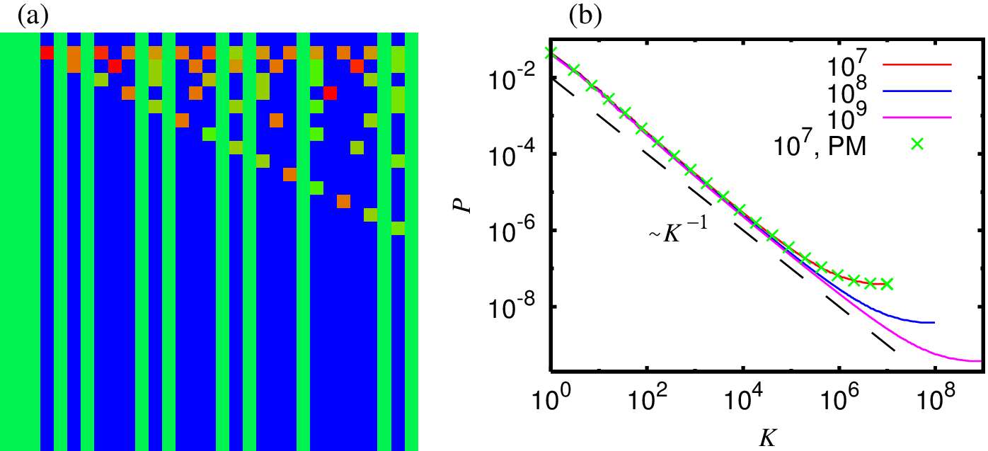
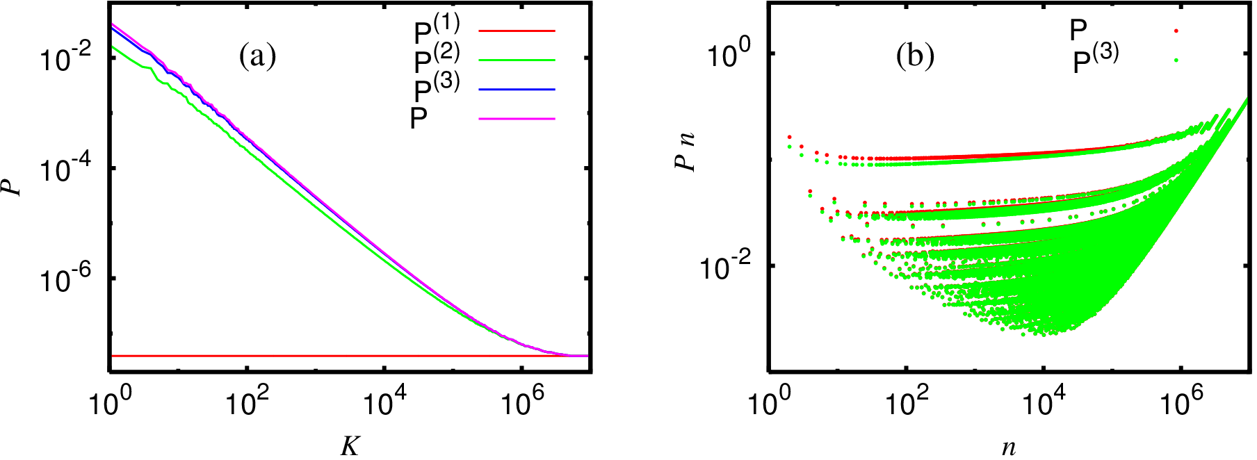
The large values of $N$ are possible because the vector iteration $v^{(j+1)}=S_{0}\,v^{(j)}$ can actually be computed without storing the $N_{\ell}\sim N\ln N$ non-vanishing elements of $S_{0}$ by using the relation:

$$v^{(j+1)}_{n}=\sum_{m=2}^{[N/n]}\,\frac{M(mn,m)}{Q(mn)}\,v^{(j)}_{mn}\;,\quad{\rm if}\ n\geq 2$$ (13)

and $v^{(j+1)}_{1}=0$ Frahm et al. (2012a). The initial vector is given by $v^{(0)}=e/N$ and $Q(n)=\sum_{m=2}^{n-1}M(n,m)$ is the number of divisors of $n$ (taking into account the multiplicity). The multiplicity $M(mn,n)$ can be recalculated during each iteration and one needs only to store $N(\ll N_{\ell})$ integer numbers $Q(n)$. It is also possible to reformulate (13) in a different way without using $M(mn,n)$ Frahm et al. (2012a). The vectors $v^{(j)}$ allow to compute the coefficients $c_{j}=d^{\,T}v^{(j)}$ in the reduced polynomial and the PageRank $P\propto\sum_{j=0}^{l-1}v^{(j)}$. Fig. 42(b) shows the PageRank for $N\in\{10^{7},\,10^{8},\,10^{9}\}$ obtained in this way and for comparison also the result of the power method for $N=10^{7}$.

Actually Fig. 43 shows that in the sum $P\propto\sum_{j=0}^{l-1}v^{(j)}$ already the first three terms give a quite satisfactory approximation to the PageRank allowing a further analytical simplified evaluation Frahm et al. (2012a) with the result $P(n)\approx C_{N}/(b_{n}\,n)$ for $n\ll N$, where $C_{N}$ is the normalization constant and $b_{n}=2$ for prime numbers $n$ and $b_{n}=6-\delta_{p_{1},p_{2}}$ for numbers $n=p_{1}\,p_{2}$ being a product of two prime numbers $p_{1}$ and $p_{2}$. The behavior $P(n)\,n\approx C_{N}/b_{n}$, which takes approximately constant values on several branches, is also visible in Fig. 43 with $C_{N}/b_{n}$ decreasing if $n$ is a product of many prime numbers. The numerical results up to $N=10^{9}$ show that the numbers $n$, corresponding to the leading PageRank values for $K=1,\,2,\,\ldots,\,32$, are $n=2$, $3$, $5$, $7$, $4$, $11$, $13$, $17$, $6$, $19$, $9$, $23$, $29$, $8$, $31$, $10$, $37$, $41$, $43$, $14$, $47$, $15$, $53$, $59$, $61$, $25$, $67$, $12$, $71$, $73$, $22$, $21$ with about 30% of non-primes among these values Frahm et al. (2012a).

A simplified model for the network for integer numbers with $M(n,m)=1$ if m is divisor of n and $1<m<n$ has also been studied with similar results Frahm et al. (2012a).

XII.3 Citation network of Physical Review

Citation networks for Physical Review and other scientific journals can be defined by taking published articles as nodes and linking an article A to another article B if A cites B. PageRank and similar analysis of such networks are efficient to determine influential articles Redner (1998); Newman (2001); Redner (2005); Radicchi et al. (2009).

In citation network links go mostly from newer to older articles and therefore such networks have, apart from the dangling node contributions, typically also a (nearly) triangular structure as can be seen in Fig. 44 which shows a coarse-grained density of the corresponding Google matrix for the citation network of Physical Review from the very beginning until 2009 Frahm et al. (2014b). However, due to the delay of the publication process in certain rare instances a published paper may cite another paper that is actually published a little later and sometimes two papers may even cite mutually each other. Therefore the matrix structure is not exactly triangular but in the coarse-grained density in Fig. 44 the rare “future citations” are not well visible.

The nearly triangular matrix structure implies large dimensional Jordan blocks associated to the eigenvalue $\lambda=0$. This creates the Jordan error enhancement (12) with severe numerical problems for accurate computation of eigenvalues in the range $|\lambda|<0.3-0.4$ when using the Arnoldi method with standard double-precision arithmetic Frahm et al. (2014b).

Figure 44: (Color online) Different representations of the Google matrix structure for the Physical Review network until 2009. (a) Density of matrix elements $G_{tt^{\prime}}$ in the basis of the publication time index $t$ (and $t^{\prime}$). (b) Density of matrix elements in the basis of journal ordering according to: Phys. Rev. Series I, Phys. Rev., Phys. Rev. Lett., Rev. Mod. Phys., Phys. Rev. A, B, C, D, E, Phys. Rev. STAB and Phys. Rev. STPER. and with time index ordering inside each journal. Note that the journals Phys. Rev. Series I, Phys. Rev. STAB and Phys. Rev. STPER are not clearly visible due to a small number of published papers. Also Rev. Mod. Phys. appears only as a thick line with 2-3 pixels (out of 500) due to a limited number of published papers. The different blocks with triangular structure correspond to clearly visible seven journals with considerable numbers of published papers. Both panels show the coarse-grained density of matrix elements on $500\times 500$ square cells for the entire network. Color shows the density of matrix elements (of $G$ at $\alpha=1$) changing from blue/black for minimum zero value to red/gray at maximum value. After Frahm et al. (2014b).

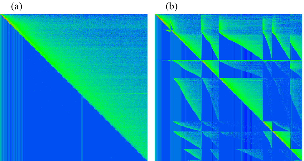
One can eliminate the small number of future citations ($12126$ which is $0.26$ % of the total number of links $N_{\ell}=4691015$) and determine the complex eigenvalue spectrum of a triangular reduced citation network using the semi-analytical theory presented in previous subsection. It turns out that in this case the matrix $S_{0}$ is nilpotent $S_{0}^{l}=0$ with $l=352$ which is much smaller than the total network size $N=463348$. The 352 non-vanishing eigenvalues can be determined numerically as the zeros of the polynomial (11) but due to an alternate sign problem with a strong loss of significance it is necessary to use the high precision library GMP with 256 binary digits Frahm et al. (2014b).

The semi-analytical theory can also be generalized to the case of nearly triangular networks, i.e. the full citation network including the future citations. In this case the matrix $S_{0}$ is no longer nilpotent but one can still generalize the arguments of previous subsection and discuss the two cases where the quantity $C=d^{\,T}\,\psi$ either vanishes (eigenvectors of first group) or is different from zero (eigenvectors of second group). The eigenvalues $\lambda$ for the first group, which may now be different from zero, can be determined by a quite complicated but numerically very efficient procedure using the subspace eigenvalues of $S$ and degenerate subspace eigenvalues of $S_{0}$ (due to absence of dangling node contributions the matrix $S_{0}$ produces much larger invariant subspaces than $S$) Frahm et al. (2014b). The eigenvalues of the second group are given as the complex zeros of the rational function:

$${\cal R}(\lambda)=1-d^{\,T}\frac{\openone}{\lambda\openone-S_{0}}e/N=1-\sum_{j=0}^{\infty}c_{j}\lambda^{-1-j}$$ (14)

with $c_{j}$ given as in (11) and now the series is not finite since $S_{0}$ is not nilpotent. For the citation network of Physical Review the coefficients $c_{j}$ behave as $c_{j}\propto\rho_{1}^{j}$ where $\rho_{1}\approx 0.902$ is the largest eigenvalue of the matrix $S_{0}$ with an eigenvector non-orthogonal to $d$. Therefore the series in (14) converges well for $|\lambda|>\rho_{1}$ but in order to determine the spectrum the rational function ${\cal R}(\lambda)$ needs to be evaluated for smaller values of $|\lambda|$. This problem can be solved by interpolating ${\cal R}(\lambda)$ with (another) rational function using a certain number of support points on the complex unit circle, where (14) converges very well, and determining the complex zeros, well inside the unit circle, of the numerator polynomial using again the high precision library GMP Frahm et al. (2014b). In this way using 16384 binary digits one may obtain 2500 reliable eigenvalues of the second group.

Figure 45: (Color online) (a) Most accurate spectrum of eigenvalues for the full Physical Review network; red/gray dots represent the core space eigenvalues obtained by the rational interpolation method with the numerical precision of $p=16384$ binary digits, $n_{R}=2500$ eigenvalues; green (light gray) dots show the degenerate subspace eigenvalues of the matrix $S_{0}$ which are also eigenvalues of $S$ with a degeneracy reduced by one (eigenvalues of the first group); blue/black dots show the direct subspace eigenvalues of $S$. (b) Spectrum of numerically accurate 352 non-vanishing eigenvalues of the Google matrix for the triangular reduced Physical Review network determined by the Newton-Maehly method applied to the reduced polynomial (11) with a high-precision calculation of 256 binary digits; note the absence of subspace eigenvalues for this case. In both panels the green/gray curve represents the unit circle. After Frahm et al. (2014b).

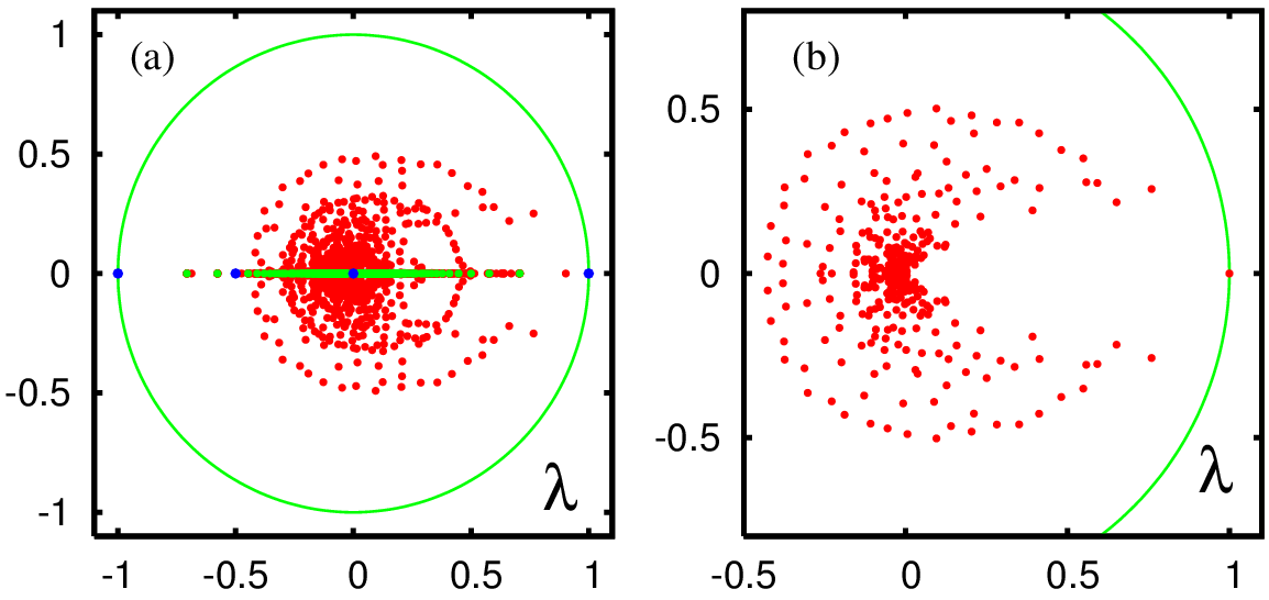
The numerical high precision spectra obtained by the semi-analytic methods for both cases, triangular reduced and full citation network, are shown in Fig. 45. One may mention that it is also possible to implement the Arnoldi method using the high precision library GMP for both cases and the resulting eigenvalues coincide very accurately with the semi-analytic spectra for both cases Frahm et al. (2014b).

When the spectrum of $G$ is determined with a good accuracy we can test the validity of the fractal Weyl law (5) changing the matrix size $N_{t}$ by considering articles published from the beginning to a certain time moment $t$ measured in years. The data presented in Fig. 46 show that the network size grows approximately exponentially as $N_{t}=2^{(t-t_{0})/\tau}$ with the fit parameters $t_{0}=1791$, $\tau=11.4$. The time interval considered in Fig. 46 is $1913\leq t\leq 2009$ since the first data point corresponds to $t=1913$ with $N_{t}=1500$ papers published between 1893 and 1913. The results, for the number $N_{\lambda}$ of eigenvalues with $|\lambda_{i}|>\lambda$, show that its growth is well described by the relation $N_{\lambda}=a\,(N_{t})^{\nu}$ for the range when the number of articles becomes sufficiently large $3\times 10^{4}\leq N_{t}<5\times 10^{5}$. This range is not very large and probably due to that there is a certain dependence of the exponent $\nu$ on the range parameter $\lambda_{c}$. At the same time we note that the maximal matrix size $N$ studied here is probably the largest one used in numerical studies of the fractal Weyl law. We have $0.47<\nu<0.6$ for all $\lambda_{c}\geq 0.4$ that is definitely smaller than unity and thus the fractal Weyl law is well applicable to the Phys. Rev. network. The value of $\nu$ increases up to $0.7$ for the data points with $\lambda_{c}<0.4$ but this is due to the fact here $N_{\lambda}$ also includes some numerically incorrect eigenvalues related to the numerical instability of the Arnoldi method at standard double-precision (52 binary digits) as discussed above.

We conclude that the most appropriate choice for the description of the data is obtained at $\lambda_{c}=0.4$ which from one side excludes small, partly numerically incorrect, values of $\lambda$ and on the other side gives sufficiently large values of $N_{\lambda}$. Here we have $\nu=0.49\pm 02$ corresponding to the fractal dimension $d=0.98\pm 0.04$. Furthermore, for $0.4\leq\lambda_{c}\leq 0.7$ we have a rather constant value $\nu\approx 0.5$ with $d_{f}\approx 1.0$. Of course, it would be interesting to extend this analysis to a larger size $N$ of citation networks of various type and not only for Phys. Rev. We expect that the fractal Weyl law is a generic feature of citation networks.

Further studies of the citation network of Physical Review concern the properties of eigenvectors (different from the PageRank) associated to relatively large complex eigenvalues, the fractal Weyl law, the correlations between PageRank and CheiRank (see also subsection IV.3) and the notion of “ImpactRank” Frahm et al. (2014b). To define the ImpactRank one may ask the question how a paper influences or has been influenced by other papers. For this one considers an initial vector $v_{0}$, localized on a one node/paper. Then the modified Google matrix $\tilde{G}=\gamma\,G+(1-\gamma)\,v_{0}\,e^{T}$ (with a damping factor $\gamma\sim 0.5-0.9$) produces a “PageRank” $v_{f}$ by the propagator $v_{f}=(1-\gamma)/(1-\gamma G)\,v_{0}$. In the vector $v_{f}$ the leading nodes/papers have strongly influenced the initial paper represented in $v_{0}$. Doing the same for $G^{*}$ one obtains a vector $v_{f}^{*}$ where the leading papers have been influenced by the initial paper represented in $v_{0}$. This procedure has been applied to certain historically important papers Frahm et al. (2014b).

Figure 46: (Color online) Data for the whole CNPR at different moments of time. Panel (a) (or (c)): shows the number $N_{\lambda}$ of eigenvalues with $\lambda_{c}\leq\lambda\leq 1$ for $\lambda_{c}=0.50$ (or $\lambda_{c}=0.65$) versus the effective network size $N_{t}$ where the nodes with publication times after a cut time $t$ are removed from the network. The green/gray line shows the fractal Weyl law $N_{\lambda}=a\,(N_{t})^{\nu}$ with parameters $a=0.32\pm 0.08$ ($a=0.24\pm 0.11$) and $\nu=0.51\pm 0.02$ ($b=0.47\pm 0.04$) obtained from a fit in the range $3\times 10^{4}\leq N_{t}<5\times 10^{5}$. The number $N_{\lambda}$ includes both exactly determined invariant subspace eigenvalues and core space eigenvalues obtained from the Arnoldi method with double-precision (52 binary digits) for $n_{A}=4000$ (red/gray crosses) and $n_{A}=2000$ (blue/black squares). Panel (b): exponent $b$ with error bars obtained from the fit $N_{\lambda}=a\,(N_{t})^{\nu}$ in the range $3\times 10^{4}\leq N_{t}<5\times 10^{5}$ versus cut value $\lambda_{c}$. Panel (d): effective network size $N_{t}$ versus cut time $t$ (in years). The green/gray line shows the exponential fit $2^{(t-t_{0})/\tau}$ with $t_{0}=1791\pm 3$ and $\tau=11.4\pm 0.2$ representing the number of years after which the size of the network (number of papers published in all Physical Review journals) is effectively doubled. After Frahm et al. (2014b).

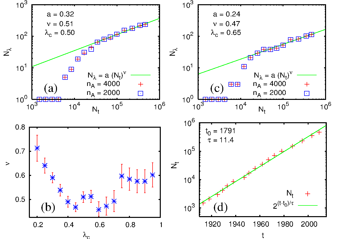
In summary, the results of this section show that the phenomenon of the Jordan error enhancement (12), induced by finite accuracy of computations with a finite number of digits, can be resolved by advanced numerical methods described above. Thus the accurate eigenvalues $\lambda$ can be obtained even for the most difficult case of quasi-triangular matrices. We note that for other networks like WWW of UK universities, Wikipedia and Twitter the triangular structure of $S$ is much less pronounced (see e.g. Fig. 1) that gives a reduction of Jordan blocks so that the Arnoldi method with double precision computes accurate values of $\lambda$.

XIII Random matrix models of Markov chains

XIII.1 Albert-Barabási model of directed networks

There are various preferential attachment models generating complex scale-free networks (see e.g. Albert and Barabási (2002); Dorogovtsev (2010)). Such undirected networks are generated by the Albert-Barabási (AB) procedure Albert and Barabási (2000) which builds networks by an iterative process. Such a procedure has been generalized to generate directed networks in Giraud et al. (2009) with the aim to study properties of the Google matrix of such networks. The procedure is working as follows: starting from $m$ nodes, at each step $m$ links are added to the existing network with probability $p$, or $m$ links are rewired with probability $q$, or a new node with $m$ links is added with probability $1-p-q$. In each case the end node of new links is chosen with preferential attachment, i.e. with probability $(k_{i}+1)/\sum_{j}(k_{j}+1)$ where $k_{i}$ is the total number of ingoing and outgoing links of node $i$. This mechanism generates directed networks having the small-world and scale-free properties, depending on the values of $p$ and $q$. The results are averaged over $N_{r}$ random realizations of the network to improve the statistics.

The studies Giraud et al. (2009) are done mainly for $m=5$, $p=0.2$ and two values of $q$ corresponding to scale-free ($q=0.1$) and exponential ($q=0.7$) regimes of link distributions (see Fig. 1 in Albert and Barabási (2000) for undirected networks). For the generated directed networks at $q=0.1$, one finds properties close to the behavior for the WWW with the cumulative distribution of ingoing links showing algebraic decay $P_{c}^{\rm\,in}(k)\sim 1/k$ and average connectivity $\langle k\rangle\approx 6.4$. For $q=0.7$ one finds $P_{c}^{\rm\,in}(k)\sim\exp(-0.03k)$ and $\langle k\rangle\approx 15$. For outgoing links, the numerical data are compatible with an exponential decay in both cases with $P_{c}^{\rm\,out}(k)\sim\exp(-0.6k)$ for $q=0.1$ and $P_{c}^{\rm\,out}(k)\sim\exp(-0.1k)$ for $q=0.7$. It is found that small variations of parameters $m,p,q$ near the chosen values do not qualitatively affect the properties of $G$ matrix.

It is found that the eigenvalues of $G$ for the AB model have one $\lambda=1$ with all other $|\lambda_{i}|<0.3$ at $\alpha=0.85$ (see Fig. 1 in Giraud et al. (2009)). This distribution shows no significant modification with the growth of matrix size $2^{10}\leq N\leq 2^{14}$. However, the values of IPR $\xi$ are growing with $N$ for typical values $|\lambda|\sim 0.2$. This indicates a delocalization of corresponding eigenstates at large $N$. At the same time the PageRank probability is well described by the algebraic dependence $P\sim 1/K$ with $\xi$ being practically independent of $N$.

These results for directed AB model network shows that it captures certain features of real directed networks, as e.g. a typical PageRank decay with the exponent $\beta\approx 1$. However, the spectrum of $G$ in this model is characterized by a large gap between $\lambda=1$ and other eigenvalues which have $\lambda\leq 0.35$ at $\alpha=1$. This feature is in a drastic difference with spectra of such typical networks at WWW of universities, Wikipedia and Twitter (see Figs. 17,22,32). In fact the AB model has no subspaces and no isolated or weakly coupled communities. In this network all sites can be reached from a given site in a logarithmic number of steps that generates a large gap in the spectrum of Google matrix and a rapid relaxation to PageRank eigenstate. In real networks there are plenty of isolated or weakly coupled communities and the introduction of damping factor $\alpha<1$ is necessary to have a single PageRank eigenvalue at $\lambda=1$. Thus the results obtained in Giraud et al. (2009) show that the AB model is not able to capture the important spectral features of real networks.

Additional studies in Giraud et al. (2009) analyzed the model of a real WWW university network with rewiring procedure of links, which consists in randomizing the links of the network keeping fixed the number of links at any given node. Starting from a single network, this creates an ensemble of randomized networks of same size, where each node has the same number of ingoing and outgoing links as for the original network. The spectrum of such randomly rewired networks is also characterized by a large gap in the spectrum of $G$ showing that rewiring destroys the communities existing in original networks. The spectrum and eigenstate properties are studied in the related work on various real networks of moderate size $N<2\times 10^{4}$ which have no spectral gap Georgeot et al. (2010).

XIII.2 Random matrix models of directed networks

Above we saw that the standard models of scale-free networks are not able to reproduce the typical properties of spectrum of Google matrices of real large scale networks. At the same time we believe that it is important to find realistic matrix models of WWW and other networks. Here we discuss certain results for certain random matrix models of $G$.

Analytical and numerical studies of random unistochastic or orthostochastic matrices of size $N=3$ and $4$ lead to triplet and cross structures in the complex eigenvalue spectra Zyczkowski et al. (2003) (see also Fig. 18). However, the size of such matrices is too small.

Here we consider other examples of random matrix models of Perron-Frobenius operators characterized by non-negative matrix elements and column sums normalized to unity. We call these models Random Perron-Frobenius Matrices (RPFM). A number of RPFM, with arbitrary size $N$, can be constructed by drawing $N^{2}$ independent matrix elements $0\leq G_{ij}\leq 1$ from a given distribution $p(G_{ij})$ with finite variance $\sigma^{2}=\langle G_{ij}^{2}\rangle-\langle G_{ij}\rangle^{2}$ and normalizing the column sums to unity Frahm et al. (2014b). The average matrix $\langle G_{ij}\rangle=1/N$ is just a projector on the vector $e$ (with unity entries on each node, see also Sec. XII.1) and has the two eigenvalues $\lambda_{1}=1$ (of multiplicity $1$) and $\lambda_{2}=0$ (of multiplicity $N-1$). Using an argument of degenerate perturbation theory on $\delta G=G-\langle G\rangle$ and known results on the eigenvalue density of non-symmetric random matrices Akemann et al. (2011); Guhr et al. (1998); Mehta (2004) one finds that an arbitrary realization of $G$ has the leading eigenvalue $\lambda_{1}=1$ and the other eigenvalues are uniformly distributed on the complex unit circle of radius $R=\sqrt{N}\sigma$ (see Fig. 47).

Figure 47: (Color online) Panel $(a)$ shows the spectrum (red/gray dots) of one realization of a full uniform RPFM with dimension $N=400$ and matrix elements uniformly distributed in the interval $[0,2/N]$; the blue/black circle represents the theoretical spectral border with radius $R=1/\sqrt{3N}\approx 0.02887$. The unit eigenvalue $\lambda=1$ is not shown due to the zoomed presentation range. Panel $(c)$ shows the spectrum of one realization of triangular RPFM (red/gray crosses) with non-vanishing matrix elements uniformly distributed in the interval $[0,2/(j-1)]$ and a triangular matrix with non-vanishing elements $1/(j-1)$ (blue/black squares); here $j=2,3,\ldots,N$ is the index-number of non-empty columns and the first column with $j=1$ corresponds to a dangling node with elements $1/N$ for both triangular cases. Panels $(b),(d)$ show the complex eigenvalue spectrum (red/gray dots) of a sparse RPFM with dimension $N=400$ and $Q=20$ non-vanishing elements per column at random positions. Panel $(b)$ (or $(d)$) corresponds to the case of uniformly distributed non-vanishing elements in the interval $[0,2/Q]$ (constant non-vanishing elements being $1/Q$); the blue/black circle represents the theoretical spectral border with radius $R=2/\sqrt{3Q}\approx 0.2582$ ($R=1/\sqrt{Q}\approx 0.2236$). In panels $(b),(d)$ $\lambda=1$ is shown by a larger red dot for better visibility. The unit circle is shown by green/gray curve (panels $(b),(c),(d)$). After Frahm et al. (2014b).

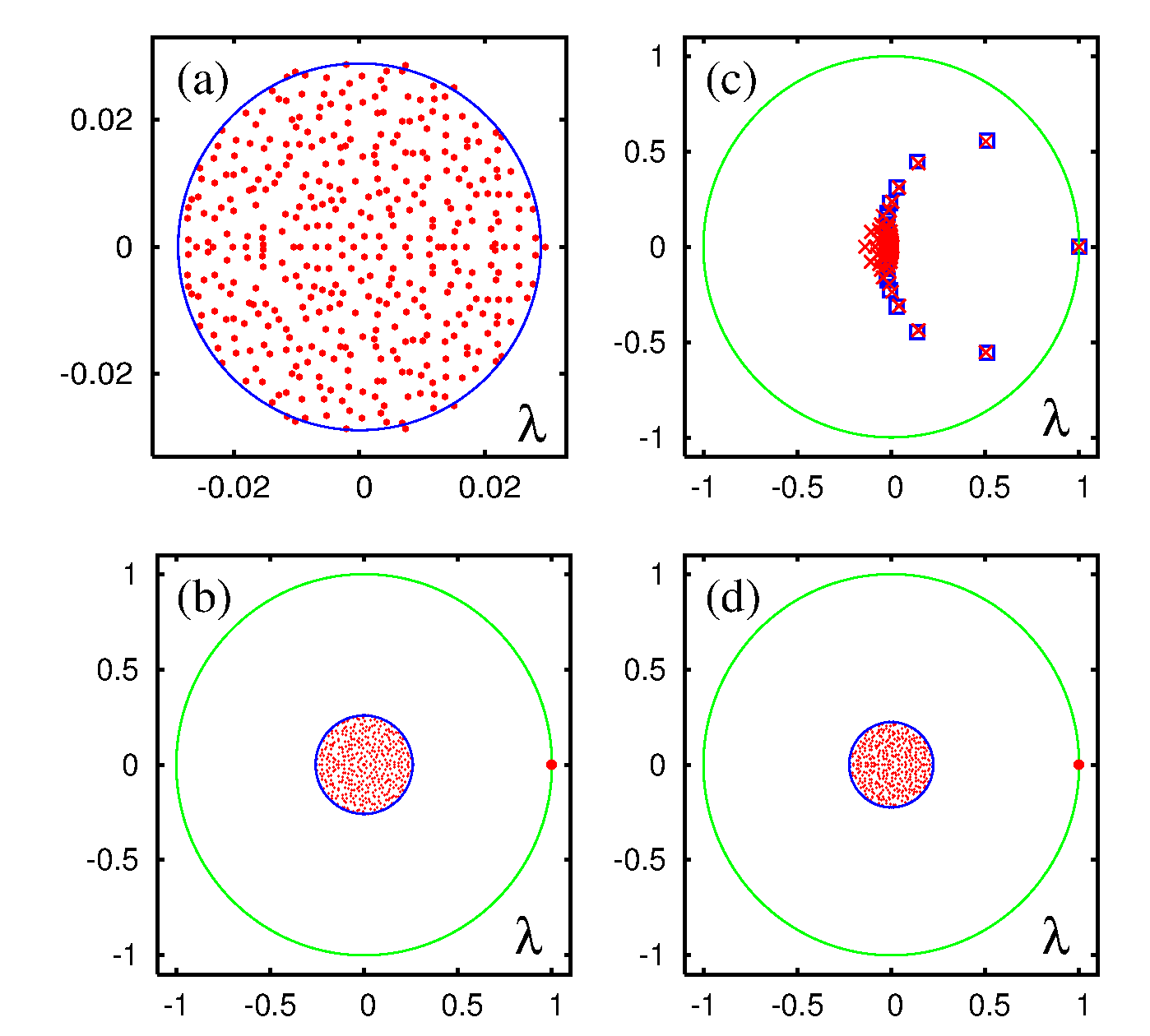
Choosing different distributions $p(G_{ij})$ one obtains different variants of the model Frahm et al. (2014b), for example $R=1/\sqrt{3N}$ using a full matrix with uniform $G_{ij}\in[0,\,2/N]$. Sparse models with $Q\ll N$ non-vanishing elements per column can be modeled by a distribution where the probability of $G_{ij}=0$ is $1-Q/N$ and for non-zero $G_{ij}$ (either uniform in $[0,\,2/Q]$ or constant $1/Q$) is $Q/N$ leading to $R=2/\sqrt{3Q}$ (for uniform non-zero elements) or $R=1/\sqrt{Q}$ (for constant non-zero elements). The circular eigenvalue density with these values of $R$ is also very well confirmed by numerical simulations in Fig. 47. Another case is a power law $p(G)=D/(1+aG)^{-b}$ (for $0\leq G\leq 1$) with $D$ and $a$ to be determined by normalization and the average $\langle G_{ij}\rangle=1/N$. For $b>3$ this case is similar to a full matrix with $R\sim 1/\sqrt{N}$. However for $2<b<3$ one finds that $R\sim N^{1-b/2}$.

The situation changes when one imposes a triangular structure on $G$ in which case the complex spectrum of $\langle G\rangle$ is already quite complicated and, due to non-degenerate perturbation theory, close to the spectrum of $G$ with modest fluctuations, mostly for the smallest eigenvalues Frahm et al. (2014b). Following the above discussion about triangular networks (with $G_{ij}=0$ for $i\geq j$) we also study numerically a triangular RPFM where for $j\geq 2$ and $i<j$ the matrix elements $G_{ij}$ are uniformly distributed in the interval $[0,2/(j-1)]$ and for $i\geq j$ we have $G_{ij}=0$. Then the first column is empty, that means it corresponds to a dangling node and it needs to be replaced by $1/N$ entries. For the triangular RPFM the situation changes completely since here the average matrix $\langle G_{ij}\rangle=1/(j-1)$ (for $i<j$ and $j\geq 2$) has already a nontrivial structure and eigenvalue spectrum. Therefore the argument of degenerate perturbation theory which allowed to apply the results of standard full non-symmetric random matrices does not apply here. In Fig. 47 one clearly sees that for $N=400$ the spectra for one realization of a triangular RPFM and its average are very similar for the eigenvalues with large modulus but both do not have at all a uniform circular density in contrast to the RPRM models without the triangular constraint discussed above. For the triangular RPFM the PageRank behaves as $P(K)\sim 1/K$ with the ranking index $K$ being close to the natural order of nodes $\{1,2,3,\ldots\}$ that reflects the fact that the node 1 has the maximum of $N-1$ incoming links etc.

The above results show that it is not so simple to propose a good random matrix model which captures the generic spectral features of real directed networks. We think that investigations in this direction should be continued.

XIII.3 Anderson delocalization of PageRank?

The phenomenon of Anderson localization of electron transport in disordered materials Anderson (1958) is now a well-known effect studied in detail in physics (see e.g. Evers and Mirlin (2008)). In one and two dimensions even a small disorder leads to an exponential localization of electron diffusion that corresponds to an insulating phase. Thus, even if a classical electron dynamics is diffusive and delocalized over the whole space, the effects of quantum interference generates a localization of all eigenstates of the Schödinger equation. In higher dimensions a localization is preserved at a sufficiently strong disorder, while a delocalized metallic phase appears for a disorder strength being smaller a certain critical value dependent on the Fermi energy of electrons. This phenomenon is rather generic and we can expect that a somewhat similar delocalization transition can appear in the small-world networks.

Figure 48: (Color online) (a) The red/gray and blue/black curves represent the Poisson and Wigner surmise distributions. Diamonds, triangles, circles and black disks represent respectively the level spacing statistics $p(s)$ at $W/V=4,3,2,1$; $p_{\ell}=0.02$, $L=32000$; averaging is done over $60$ network realizations. (b) Stars give dependence of $p_{\ell}$ on a disorder strength $W/V$ at the critical point when $\eta_{\ell}(W,p_{\ell})=0.8$, and $p_{\ell}=0.005,0.01,0.02,0.04$ at fixed $L=8000$; the straight line corresponds to $p_{\ell}=p_{c}=1/4\ell_{1}\approx(W/V)^{2}/400$; the dashed curve is drown to adapt an eye. After Chepelianskii and Shepelyansky (2001).

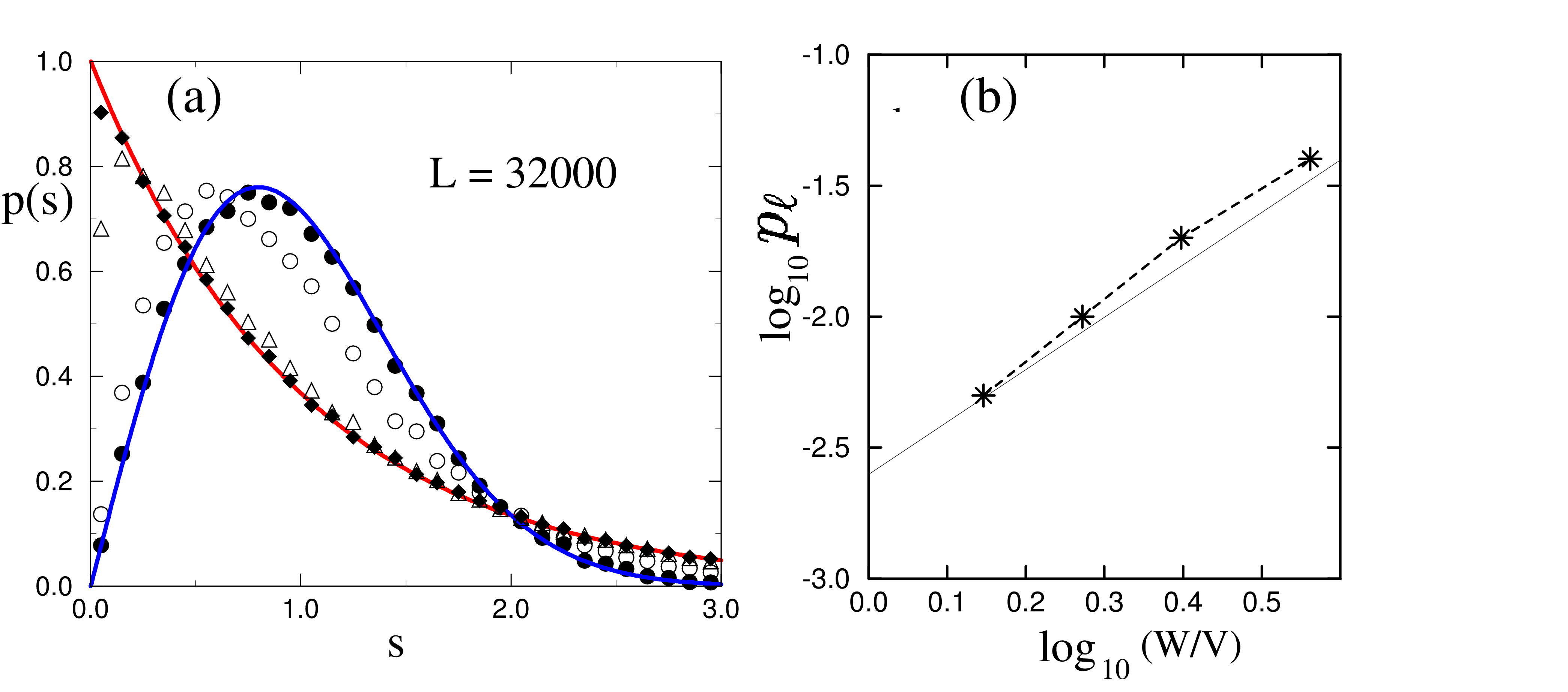
Indeed, it is useful to consider the $1D$ Anderson model on a ring with a certain number of shortcut links, described by the Schödinger equation

$$\epsilon_{n}\psi_{n}+V(\psi_{n+1}+\psi_{n-1})+V\sum_{S}(\psi_{n+S}+\psi_{n-S})=E\psi_{n}\;,$$ (15)

where $\epsilon_{n}$ are random on site energies homogeneously distributed within the interval $-W/2\leq\epsilon_{n}\leq W/2$, and $V$ is the hopping matrix element. The sum over $S$ is taken over randomly established shortcuts from a site $n$ to any other random site of the network. The number of such shortcuts is $S_{\rm tot}=p_{\ell}L$, where $L$ is the total number of sites on a ring and $p_{\ell}$ is the density of shortcut links. This model had been introduced in Chepelianskii and Shepelyansky (2001). The numerical study, reported there, showed that the level-spacing statistics $p(s)$ for this model has a transition from the Poisson distribution $p_{\rm Pois}(s)=\exp(-s)$, typical for the Anderson localization phase, to the Wigner surmise distribution $p_{\rm Wig}(s)=\pi s/2\exp(-\pi s^{2}/4)$, typical for the Anderson metallic phase Guhr et al. (1998); Evers and Mirlin (2008). The numerical diagonalization was done via the Lanczos algorithm for the sizes up to $L=32000$ and the typical parameter range $0.005\leq p_{\ell}<0.1$ and $1\leq W/V\leq 4$. An example, of the variation of $p_{\ell}(s)$ with a decrease of $W/V$ is shown in Fig. 48(a). We see that the Wigner surmise provides a good description of the numerical data at $W/V=1$, when the maximal localization length $\ell_{1}\approx 96(V/W)^{2}\approx 96$ in the 1D Anderson model (see e.g. Evers and Mirlin (2008)) is much smaller than the system size $L$.

To identify a transition from one limiting case $p_{\rm Pois}(s)$ to another $p_{\rm Wig}(s)$ it is convenient to introduce the parameter $\eta_{s}=\int_{0}^{s_{0}}(p(s)-p_{\rm Wig}(s))ds/\int_{0}^{s_{0}}(p_{\rm Pois}(s)-p_{\rm Wig}(s))ds$, where $s_{0}=0.4729...$ is the intersection point of $p_{\rm Pois}(s)$ and $p_{\rm Wig}(s)$. In this way $\eta_{s}$ varies from $1$ (for $p(s)=p_{\rm Pois}(s)$) to $0$ (for $p(s)=p_{\rm Wig}(s)\;$) (see e.g. Shepelyansky (2001)). From the variation of $\eta_{s}$ with system parameters and size $L$, the critical density $p_{\ell}=p_{c}$ can be determined by the condition $\eta_{s}(p_{c},W/V)=\eta_{c}=0.8=const.$ being independent of $L$. The obtained dependence of $p_{c}$ on $W/V$ obtained at a fixed critical point $\eta_{c}=0.8$ is shown in Fig. 48(b). The Anderson delocalization transition takes place when the density of shortcuts becomes larger than a critical density $p_{\ell}>p_{c}\approx 1/(4\ell_{1})$ where $\ell_{1}\approx 96(V/W)^{2}$ is the length of Anderson localization in $1D$. A simple physical interpretation of this result is that the delocalization takes place when the localization length $\ell_{1}$ becomes larger than a typical distance $1/(4p_{\ell})$ between shortcuts. The further studies of time evolution of wave function $\psi_{n}(t)$ and IPR $\xi$ variation also confirmed the existence of quantum delocalization transition on this quantum small-world network Giraud et al. (2005).

Thus the results obtained for the quantum small-world networks Chepelianskii and Shepelyansky (2001); Giraud et al. (2005) show that the Anderson transition can take place in such systems. However, the above model represents an undirected network corresponding to a symmetric matrix with a real spectrum while the typical directed networks are characterized by asymmetric matrix $G$ and complex spectrum. The possibility of existence of localized states of $G$ for WWW networks was also discussed by Perra et al. (2009) but the fact that in a typical case the spectrum of $G$ is complex has not been analyzed in detail.

Above we saw certain indications on a possibility of Anderson type delocalization transition for eigenstates of the $G$ matrix. Our results clearly show that certain eigenstates in the core space are exponentially localized (see e.g. Fig 19(b)). Such states are localized only on a few nodes touching other nodes of network only by an exponentially small tail. A similar situation would appear in the 1D Anderson model if an absorption would be introduced on one end of the chain. Then the eigenstates located far away from this place would feel this absorption only by exponentially small tails so that the imaginary part of the eigenenergy would have for such far away states only an exponentially small imaginary part. It is natural to expect that such localization can be destroyed by some parameter variation. Indeed, certain eigenstates with $|\lambda|<1$ for the directed network of the AB model have IPR $\xi$ growing with the matrix size $N$ (see Sec. XIII.1 and Giraud et al. (2009)) even if for the PageRank the values of $\xi$ remain independent of $N$. The results for the Ulam network from Figs. 13, 14 provide an example of directed network where the PageRank vector becomes delocalized when the damping factor is decreased from $\alpha=0.95$ to $0.85$ Zhirov et al. (2010). This example demonstrates a possibility of PageRank delocalization but a deeper understanding of the conditions required for such a phenomenon to occur are still lacking. The main difficulty is an absence of well established random matrix models which have properties similar to the available examples of real networks.

Indeed, for Hermitian and unitary matrices the theories of random matrices, mesoscopic systems and quantum chaos allow to capture main universal properties of spectra and eigenstates Guhr et al. (1998); Akemann et al. (2011); Mehta (2004); Evers and Mirlin (2008); Haake (2010). For asymmetric Google matrices the spectrum is complex and at the moment there are no good random matrix models which would allow to perform analytical analysis of various parameter dependencies. It is possible that non-Hermitian Anderson models in $1D$, which naturally generates a complex spectrum and may have delocalized eigenstates, will provide new insights in this direction Goldsheid and Khoruzhenko (1998). We note that the recent random Google matrix models studied in Zhirov and Shepelyansky (2015) give indications on appearance of the Anderson transition for Google matrix eigenstates and a mobility edge contour in a plane of complex eigenvalues.

XIV Other examples of directed networks

In this section we discuss additional examples of real directed networks.

XIV.1 Brain neural networks

In 1958 John von Neumann traced first parallels between architecture of the computer and the brain von Neumann (1958). Since that time computers became an unavoidable element of the modern society forming a computer network connected by the WWW with about $4\times 10^{9}$ indexed web pages spread all over the world (see e.g. http://www.worldwidewebsize.com/). This number starts to become comparable with $10^{10}$ neurons in a human brain where each neuron can be viewed as an independent processing unit connected with about $10^{4}$ other neurons by synaptic links (see e.g. Sporns (2007)). About 20% of these links are unidirectional Felleman and van Essen (1991) and hence the brain can be viewed as a directed network of neuron links. At present, more and more experimental information about neurons and their links becomes available and the investigations of properties of neuronal networks attract an active interest (see e.g. Bullmore and Sporns (2009); Zuo et al. (2012)). The fact that enormous sizes of WWW and brain networks are comparable gives an idea that the Google matrix analysis should find useful application in brain science as it is the case of WWW.

First applications of methods of Google matrix methods to brain neural networks was done in Shepelyansky and Zhirov (2010b) for a large-scale thalamocortical model Izhikevich and Edelman (2008) based on experimental measures in several mammalian species. The model spans three anatomic scales. (i) It is based on global (white-matter) thalamocortical anatomy obtained by means of diffusion tensor imaging of a human brain. (ii) It includes multiple thalamic nuclei and six-layered cortical microcircuitry based on in vitro labeling and three-dimensional reconstruction of single neurons of cat visual cortex. (iii) It has 22 basic types of neurons with appropriate laminar distribution of their branching dendritic trees. According to Izhikevich and Edelman (2008) the model exhibits behavioral regimes of normal brain activity that were not explicitly built-in but emerged spontaneously as the result of interactions among anatomical and dynamic processes.

Figure 49: (Color online) (a) Spectrum of eigenvalues $\lambda$ for the Google matrices $G$ and $G^{*}$ at $\alpha=0.85$ for the neural network of C.elegans (black and red/gray symbols). (b) Values of IPR $\xi_{i}$ of eigenvectors $\psi_{i}$ are shown as a function of corresponding $Re\lambda$ (same colors). After Kandiah and Shepelyansky (2014a).

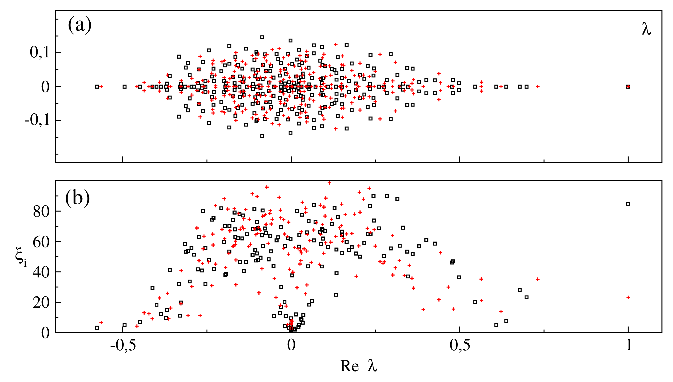
The model studied in Shepelyansky and Zhirov (2010b) contains $N=10^{4}$ neuron with $N_{\ell}=1960108$. The obtained results show that PageRank and CheiRank vectors have rather large $\xi$ being comparable with the whole network size at $\alpha=0.85$. The corresponding probabilities have very flat dependence on their indexes showing that they are close to a delocalized regime. We attribute these features to a rather large number of links per node $\zeta\approx 196$ being even larger than for the Twitter network. At the same time the PageRank-CheiRank correlator is rather small $\kappa=-0.065$. Thus this network is structured in such a way that functions related to order signals (outgoing links of CheiRank) and signals bringing orders (ingoing links of PageRank) are well separated and independent of each other as it is the case for the Linux Kernel software architecture. The spectrum of $G$ has a gapless structure showing that long living excitations can exist in this neuronal network.

Of course, model systems of neural networks can provide a number of interesting insights but it is much more important to study examples of real neural networks. In Kandiah and Shepelyansky (2014a) such an analysis is performed for the neural network of C.elegans (worm). The full connectivity of this directed network is known and well documented at WormAtlas Altun et al. (2012). The number of linked neurons (nodes) is $N=279$ with the number of synaptic connections and gap junctions (links) between them being $N_{\ell}=2990$.

Figure 50: (Color online) PageRank - CheiRank plane $(K,K^{*})$ showing distribution of neurons according to their ranking. (a): soma region coloration - head (red/gray), middle (green/light gray), tail (blue/dark gray). (b): neuron type coloration - sensory (red/gray), motor (green/light gray), interneuron (blue/dark gray), polymodal (purple/light-dark gray) and unknown (black). The classifications and colors are given according to WormAtlas Altun et al. (2012). After Kandiah and Shepelyansky (2014a).

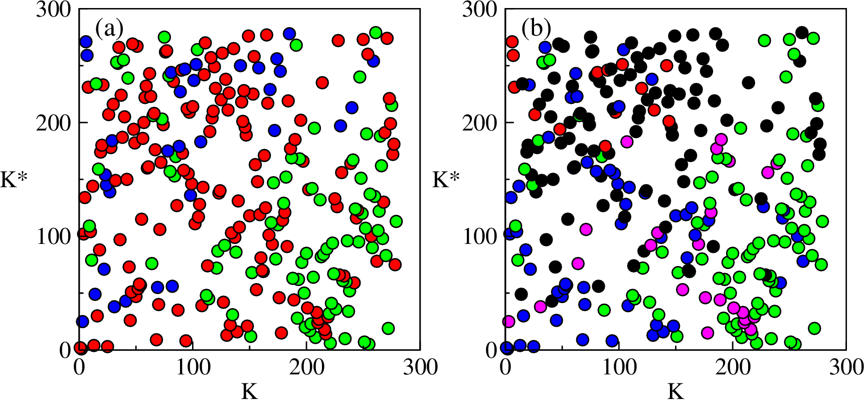
The Google matrix $G$ of C.elegans is constructed using the connectivity matrix elements $S_{ij}=S_{{\rm syn},ij}+S_{{\rm gap},ij}$, where $S_{\rm syn}$ is an asymmetric matrix of synaptic links whose elements are $1$ if neuron $j$ connects to neuron $i$ through a chemical synaptic connection and $0$ otherwise. The matrix part $S_{\rm gap}$ is a symmetric matrix describing gap junctions between pairs of cells, $S_{{\rm gap},ij}=S_{{\rm gap},ji}=1$ if neurons $i$ and $j$ are connected through a gap junction and $0$ otherwise. Then the matrices $G$ and $G^{*}$ are constructed following the standard rule (1) at $\alpha=0.85$. The connectivity properties of this network are similar to those of WWW of Cambridge and Oxford with approximately the same number of links per node.

The spectra of $G$ and $G^{*}$ are shown in Fig. 49 with corresponding IPR values of eigenstates. The imaginary part of $\lambda$ is relatively small $|{\rm Im}(\lambda)|<0.2$ due to a large fraction of symmetric links. The second by modulus eigenvalues are $\lambda_{2}=0.8214$ for $G$ and $\lambda_{2}=0.8608$ for $G^{*}$. Thus the network relaxation time $\tau=1/|\ln\lambda_{2}|$ is approximately $5,6.7$ iterations of $G,G^{*}$. Certain IPR values $\xi_{i}$ of eigenstates of $G,G^{*}$ have rather large $\xi\approx N/3$ while others have $\xi$ located only on about ten nodes.

We have a large value $\xi\approx 85$ for PageRank and a more moderate value $\xi\approx 23$ for CheiRank vectors. Here we have the algebraic decay exponents being $\beta\approx 0.33$ for $P(K)$ and $\beta\approx 0.50$ for $P^{*}(K^{*})$. Of course, the network size is not large and these values are only approximate. However, they indicate an interchange between PageRank and CheiRank showing importance of outgoing links. It is possible that such an inversion is related to a significant importance of outgoing links in neural systems: in a sense such links transfer orders, while ingoing links bring instructions to a given neuron from other neurons. The correlator $\kappa=0.125$ is small and thus, the network structure allows to perform a control of information flow in a more efficient way without interference of errors between orders and executions. We saw already in Sec. VII.1 that such a separation of concerns emerges in software architecture. It seems that the neural networks also adopt such a structure.

We note that a somewhat similar situation appears for networks of Business Process Management where Principals of a company are located at the top CheiRank position while the top PageRank positions belong to company Contacts Abel and Shepelyansky (2011). Indeed, a case study of a real company structure analyzed in Abel and Shepelyansky (2011) also stress the importance of company managers who transfer orders to other structural units. For this network the correlator is also small being $\kappa=0.164$. We expect that brain neural networks may have certain similarities with company organization.

Each neuron $i$ belongs to two ranks $K_{i}$ and $K^{*}_{i}$ and it is convenient to represent the distribution of neurons on PageRank-CheiRank plane $(K,K^{*})$ shown in Fig. 50. The plot confirms that there are little correlations between both ranks since the points are scattered over the whole plane. Neurons ranked at top $K$ positions of PageRank have their soma located mainly in both extremities of the worm (head and tail) showing that neurons in those regions have important connections coming from many other neurons which control head and tail movements. This tendency is even more visible for neurons at top $K^{*}$ positions of CheiRank but with a preference for head and middle regions. In general, neurons, that have their soma in the middle region of the worm, are quite highly ranked in CheiRank but not in PageRank. The neurons located at the head region have top positions in CheiRank and also PageRank, while the middle region has some top CheiRank indexes but rather large indexes of PageRank (Fig. 50 (a)). The neuron type coloration (Fig. 50 (b)) also reveals that sensory neurons are at top PageRank positions but at rather large CheiRank indexes, whereas in general motor neurons are in the opposite situation.

Top nodes of PageRank and CheiRank favor important signal relaying neurons such as $AVA$ and $AVB$ that integrate signals from crucial nodes and in turn pilot other crucial nodes. Neurons $AVAL,AVAR$, $AVBL,AVBR$ and $AVEL,AVER$ are considered to belong to the rich club analyzed in Towlson et al. (2013). The top neurons in 2DRank are AVAL, AVAR, AVBL, AVBR, PVCR that corresponds to a dominance of interneurons. More details can be found in Kandiah and Shepelyansky (2014a).

The technological progress allows to obtain now more and more detailed information about neural networks (see e.g. Bullmore and Sporns (2009); Towlson et al. (2013); Zuo et al. (2012)) even if it is not easy to get information about link directions. In view of that we expect that the methods of directed network analysis described here will find useful future applications for brain neural networks.

XIV.2 Google matrix of DNA sequences

The approaches of Markov chains and Google matrix can be also efficiently used for analysis of statistical properties of DNA sequences. The data sets are publicly available at Ensemble Genome database (2011). The analysis of Poincaré recurrences in these DNA sequences Frahm and Shepelyansky (2012c) shows their similarities with the statistical properties of recurrences for dynamical trajectories in the Chirikov standard map and other symplectic maps Frahm and Shepelyansky (2010). Indeed, a DNA sequence can be viewed as a long symbolic trajectory and hence, the Google matrix, constructed from it, highlights the statistical features of DNA from a new viewpoint.

An important step in the statistical analysis of DNA sequences was done in Mantegna et al. (1995) applying methods of statistical linguistics and determining the frequency of various words composed of up to 7 letters. A first order Markovian models have been also proposed and briefly discussed in this work. The Google matrix analysis provides a natural extension of this approach. Thus the PageRank eigenvector gives most frequent words of given length. The spectrum and eigenstates of $G$ characterize the relaxation processes of different modes in the Markov process generated by a symbolic DNA sequence. Thus the comparison of word ranks of different species allows to identify their proximity.

Figure 51: (Color online) DNA Google matrix of Homo sapiens (HS) constructed for words of 6-letters length. Matrix elements $G_{KK^{\prime}}$ are shown in the basis of PageRank index $K$ (and $K^{\prime}$). Here, $x$ and $y$ axes show $K$ and $K^{\prime}$ within the range $1\leq K,K^{\prime}\leq 200$ (a) and $1\leq K,K^{\prime}\leq 1000$ (b). The element $G_{11}$ at $K=K^{\prime}=1$ is placed at top left corner. Color marks the amplitude of matrix elements changing from blue/black for minimum zero value to red/gray at maximum value. After Kandiah and Shepelyansky (2013).

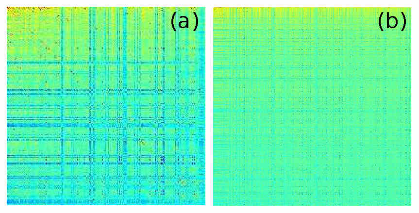
The statistical analysis is done for DNA sequences of the species: Homo sapiens (HS, human), Canis familiaris (CF, dog), Loxodonta africana (LA, elephant), Bos Taurus (bull, BT), Danio rerio (DR, zebrafish) Kandiah and Shepelyansky (2013). For HS DNA sequences are represented as a single string of length $L\approx 1.5\cdot 10^{10}$ base pairs (bp) corresponding to 5 individuals. Similar data are obtained for BT ($2.9\cdot 10^{9}$ bp), CF ($2.5\cdot 10^{9}$ bp), LA ($3.1\cdot 10^{9}$ bp), DR ($1.4\cdot 10^{9}$ bp). All strings are composed of 4 letters $A,G,G,T$ and undetermined letter ${\it N_{l}}$. The strings can be found from Kandiah and Shepelyansky (2013).

For a given sequence we fix the words $W_{k}$ of $m$ letters length corresponding to the number of states $N=4^{m}$. We consider that there is a transition from a state $j$ to state $i$ inside this basis $N$ when we move along the string from left to right going from a word $W_{k}$ to a next word $W_{k+1}$. This transition adds one unit in the transition matrix element $T_{ij}\rightarrow T_{ij}+1$. The words with letter ${\it N_{l}}$ are omitted, the transitions are counted only between nearby words not separated by words with $N_{l}$. There are approximately $N_{t}\approx L/m$ such transitions for the whole length $L$ since the fraction of undetermined letters ${\it N_{l}}$ is small. Thus we have $N_{t}=\sum_{i,j=1}^{N}T_{ij}$. The Markov matrix of transitions $S_{ij}$ is obtained by normalizing matrix elements in such a way that their sum in each column is equal to unity: $S_{ij}=T_{ij}/\sum_{i}T_{ij}$. If there are columns with all zero elements (dangling nodes) then zeros of such columns are replaced by $1/N$. Then the Google matrix $G$ is constructed from $S$ by the standard rule (1). It is found that the spectrum of $G$ has a significant gap and a variation of $\alpha$ in a range $(0.5,1)$ does not affect significantly the PageRank probability. Thus all DNA results are shown at $\alpha=1$.

Figure 52: (Color online) Integrated fraction $N_{g}/N^{2}$ of Google matrix elements with $G_{ij}>g$ as a function of $g$. (a) Various species with 6-letters word length: elephant LA (green), zebrafish DR(black), dog CF (red), bull BT (magenta), and Homo sapiens HS (blue) (from left to right at $y=-5.5$). (b) Data for HS sequence with words of length $m=5$ (brown), $6$ (blue), $7$ (red) (from right to left at $y=-2$); for comparison black dashed and dotted curves show the same distribution for the WWW networks of Universities of Cambridge and Oxford in 2006 respectively. After Kandiah and Shepelyansky (2013).

Figure 53: (Color online) Integrated fraction $N_{s}/N$ of sum of ingoing matrix elements with $\sum_{j=1}^{N}G_{i,j}\geq g_{s}$. Panels (a) and (b) show the same cases as in Fig. 52 in same colors. The dashed and dotted curves are shifted in $x$-axis by one unit left to fit the figure scale. After Kandiah and Shepelyansky (2013).

Figure 54: (Color online) Dependence of PageRank probability $P(K)$ on PageRank index $K$. (a) Data for different species for word length of 6-letters: zebrafish DR (black), dog CF (red), Homo sapiens HS (blue), elephant LA (green) and bull BT (magenta) (from top to bottom at $x=1$). (b) Data for HS (full curve) and LA (dashed curve) for word length $m=5$ (brown), $6$ (blue/green), $7$ (red) (from top to bottom at $x=1$). After Kandiah and Shepelyansky (2013).

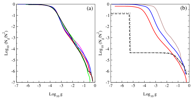
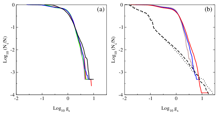
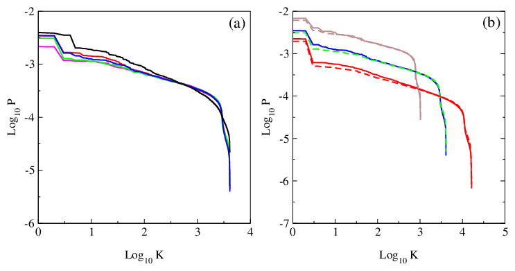
The image of matrix elements $G_{KK^{\prime}}$ is shown in Fig. 51 for HS with $m=6$. We see that almost all matrix is full that is drastically different from the WWW and other networks considered above. The analysis of statistical properties of matrix elements $G_{ij}$ shows that their integrated distribution follows a power law as it is seen in Fig. 52. Here $N_{g}$ is the number of matrix elements of the matrix $G$ with values $G_{ij}>g$. The data show that the number of nonzero matrix elements $G_{ij}$ is very close to $N^{2}$. The main fraction of elements has values $G_{ij}\leq 1/N$ (some elements $G_{ij}<1/N$ since for certain $j$ there are many transitions to some node $i^{\prime}$ with $T_{i^{\prime}j}\gg N$ and e.g. only one transition to other $i^{\prime\prime}$ with $T_{i^{\prime\prime}j}=1$). At the same time there are also transition elements $G_{ij}$ with large values whose fraction decays in an algebraic law $N_{g}\approx AN/g^{\nu-1}$ with some constant $A$ and an exponent $\nu$. The fit of numerical data in the range $-5.5<\log_{10}g<-0.5$ of algebraic decay gives for $m=6$: $\nu=2.46\pm 0.025$ (BT), $2.57\pm 0.025$ (CF), $2.67\pm 0.022$ (LA), $2.48\pm 0.024$ (HS), $2.22\pm 0.04$ (DR). For HS case we find $\nu=2.68\pm 0.038$ at $m=5$ and $\nu=2.43\pm 0.02$ at $m=7$ with the average $A\approx 0.003$ for $m=5,6,7$. There are visible oscillations in the algebraic decay of $N_{g}$ with $g$ but in global we see that on average all species are well described by a universal decay law with the exponent $\nu\approx 2.5$. For comparison we also show the distribution $N_{g}$ for the WWW networks of University of Cambridge and Oxford in year 2006. We see that in these cases the distribution $N_{g}$ has a very short range in which the decay is at least approximately algebraic ($-5.5<\log_{10}(N_{g}/N^{2})<-6$). In contrast to that for the DNA sequences we have a large range of algebraic decay.

Since in each column we have the sum of all elements equal to unity we can say that the differential fraction $dN_{g}/dg\propto 1/g^{\nu}$ gives the distribution of outgoing matrix elements which is similar to the distribution of outgoing links extensively studied for the WWW networks. Indeed, for the WWW networks all links in a column are considered to have the same weight so that these matrix elements are given by an inverse number of outgoing links with the decay exponent $\nu\approx 2.7$. Thus, the obtained data show that the distribution of DNA matrix elements is similar to the distribution of outgoing links in the WWW networks. Indeed, for outgoing links of Cambridge and Oxford networks the fit of numerical data gives the exponents $\nu=2.80\pm 0.06$ (Cambridge) and $2.51\pm 0.04$ (Oxford).

As discussed above, on average the probability of PageRank vector is proportional to the number of ingoing links that works satisfactory for sparse $G$ matrices. For DNA we have a situation where the Google matrix is almost full and zero matrix elements are practically absent. In such a case an analogue of number of ingoing links is the sum of ingoing matrix elements $g_{s}=\sum_{j=1}^{N}G_{ij}$. The integrated distribution of ingoing matrix elements with the dependence of $N_{s}$ on $g_{s}$ is shown in Fig. 53. Here $N_{s}$ is defined as the number of nodes with the sum of ingoing matrix elements being larger than $g_{s}$. A significant part of this dependence, corresponding to large values of $g_{s}$ and determining the PageRank probability decay, is well described by a power law $N_{s}\approx BN/g_{s}^{\mu-1}$. The fit of data at $m=6$ gives $\mu=5.59\pm 0.15$ (BT), $4.90\pm 0.08$ (CF), $5.37\pm 0.07$ (LA), $5.11\pm 0.12$ (HS), $4.04\pm 0.06$ (DR). For HS case at $m=5,7$ we find respectively $\mu=5.86\pm 0.14$ and $4.48\pm 0.08$. For $HS$ and other species we have an average $B\approx 1$.

For WWW one usually have $\mu\approx 2.1$. Indeed, for the ingoing matrix elements of Cambridge and Oxford networks we find respectively the exponents $\mu=2.12\pm 0.03$ and $2.06\pm 0.02$ (see curves in Fig. 53). For ingoing links distribution of Cambridge and Oxford networks we obtain respectively $\mu=2.29\pm 0.02$ and $\mu=2.27\pm 0.02$ which are close to the usual WWW value $\mu\approx 2.1$. In contrast the exponent $\mu$ for DNA Google matrix elements gets significantly larger value $\mu\approx 5$. This feature marks a significant difference between DNA and WWW networks.

The PageRank vector can be obtained by a direct diagonalization. The dependence of probability $P$ on index $K$ is shown in Fig. 54 for various species and different word length $m$. The probability $P(K)$ describes the steady state of random walks on the Markov chain and thus it gives the frequency of appearance of various words of length $m$ in the whole sequence $L$. The frequencies or probabilities of words appearance in the sequences have been obtained in Mantegna et al. (1995) by a direct counting of words along the sequence (the available sequences $L$ were shorted at that times). Both methods are mathematically equivalent and indeed our distributions $P(K)$ are in good agreement with those found in Mantegna et al. (1995) even if now we have a significantly better statistics.

Figure 55: (Color online) PageRank proximity $K-K$ plane diagrams for different species in comparison with Homo sapiens: (a) $x$-axis shows PageRank index $K_{hs}(i)$ of a word $i$ and $y$-axis shows PageRank index of the same word $i$ with $K_{bt}(i)$ of bull, (b) $K_{cf}(i)$ of dog, (c) $K_{la}(i)$ of elephant and (d) $K_{dr}(i)$ of zebrafish; here the word length is $m=6$. The colors of symbols marks the purine content in a word $i$ (fractions of letters $A$ or $G$ in any order); the color varies from red/gray at maximal content, via brown, yellow, green, light blue, to blue/black at minimal zero content. After Kandiah and Shepelyansky (2013).

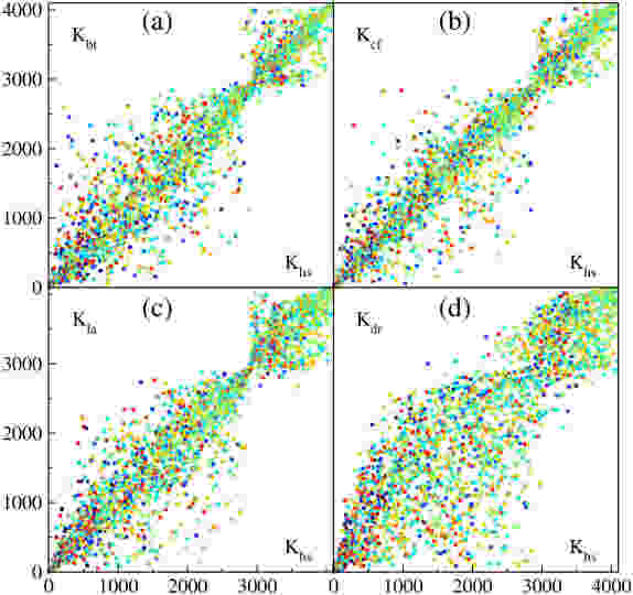
The decay of $P$ with $K$ can be approximately described by a power law $P\sim 1/K^{\beta}$. Thus for example for HS sequence at $m=7$ we find $\beta=0.357\pm 0.003$ for the fit range $1.5\leq\log_{10}K\leq 3.7$ that is rather close to the exponent found in Mantegna et al. (1995). Since on average the PageRank probability is proportional to the number of ingoing links, or the sum of ingoing matrix elements of $G$, one has the relation between the exponent of PageRank $\beta$ and exponent of ingoing links (or matrix elements): $\beta=1/(\mu-1)$. Indeed, for the HS DNA case at $m=7$ we have $\mu=4.48$ that gives $\beta=0.29$ being close to the above value of $\beta=0.357$ obtained from the direct fit of $P(K)$ dependence. The agreement is not so perfect since there is a visible curvature in the log-log plot of $N_{s}$ vs $g_{s}$ and also since a small value of $\beta$ gives a moderate variation of $P$ that produces a reduction of accuracy of numerical fit procedure. In spite of this only approximate agreement we conclude that in global the relation between $\beta$ and $\mu$ works correctly.

It is interesting to plot a PageRank index $K_{s}(i)$ of a given species $s$ versus the index $K_{hs}(i)$ of HS for the same word $i$. For identical sequences one should have all points on diagonal, while the deviations from diagonal characterize the differences between species. The examples of such PageRank proximity $K-K$ diagrams are shown in Fig. 55 for words at $m=6$. A visual impression is that CF case has less deviations from HS rank compared to BT and LA. The non-mammalian DR case has most strong deviations from HS rank.

The fraction of purine letters $A$ or $G$ in a word of $m=6$ letters is shown by color in Fig. 55 for all words ranked by PageRank index $K$. We see that these letters are approximately homogeneously distributed over the whole range of $K$ values. To determine the proximity between different species or different HS individuals we compute the average dispersion

$$\sigma(s_{1},s_{2})=\sqrt{\frac{1}{N}\sum_{i=1}^{N}\Bigl{(}K_{s_{1}}(i)-K_{s_{2}}(i)\Bigr{)}^{2}}$$ (16)

between two species (individuals) $s_{1}$ and $s_{2}$. Comparing the words with length $m=5,6,7$ we find that the scaling $\sigma\propto N$ works with a good accuracy (about 10% when $N$ is increased by a factor 16). To represent the result in a form independent of $m$ we compare the values of $\sigma$ with the corresponding random model value $\sigma_{rnd}$. This value is computed assuming a random distribution of $N$ points in a square $N\times N$ when only one point appears in each column and each line (e.g. at $m=6$ we have $\sigma_{rnd}\approx 1673$ and $\sigma_{rnd}\propto N$). The dimensionless dispersion is then given by $\zeta(s_{1},s_{2})=\sigma(s_{1},s_{2})/\sigma_{rnd}$. From the ranking of different species we obtain the following values at $m=6$: $\zeta(CF,BT)=0.308$; $\zeta(LA,BT)=0.324$, $\zeta(LA,CF)=0.303$; $\zeta(HS,BT)=0.246$, $\zeta(HS,CF)=0.206$, $\zeta(HS,LA)=0.238$; $\zeta(DR,BT)=0.425$, $\zeta(DR,CF)=0.414$, $\zeta(DR,LA)=0.422$, $\zeta(DR,HS)=0.375$ (other $m$ have similar values). According to this statistical analysis of PageRank proximity between species we find that $\zeta$ value is minimal between CF and HS showing that these are two most similar species among those considered here. The comparison of two HS individuals gives the value $\zeta(HS1,HS2)=0.031$ being significantly smaller then the proximity correlator between different species Kandiah and Shepelyansky (2012).

The spectrum of $G$ is analyzed in detail in Kandiah and Shepelyansky (2012). It is shown that it has a relatively large gap due to which there is a relatively rapid relaxation of probability of a random surfer to the PageRank values.

Figure 56: (Color online) Distribution of nodes in the PageRank-CheiRank plane $(K,K^{*})$ for Escherichia Coli v1.1 (a), and Yeast (b) gene transcription networks on (network data are taken from Shen-Orr et al. (2002); Milo et al. (2002) and Alon (2014)). The nodes with five top probability values of PageRank, CheiRank and 2DRank are labeled by their corresponding operon (node) names; they correspond to 5 lowest values of indexes $K,K_{2},K^{*}$. After Ermann et al. (2012a).

XIV.3 Gene regulation networks

At present the analysis of gene transcription regulation networks and recovery of their control biological functions becomes an active research field of bioinformatics (see e.g. Milo et al. (2002)). Here, following Ermann et al. (2012a), we provide two simple examples of 2DRanking analysis for gene transcriptional regulation networks of Escherichia Coli ($N=423$, $N_{\ell}=519$ Shen-Orr et al. (2002)) and Yeast ($N=690$, $N_{\ell}=1079$ Milo et al. (2002)). In the construction of $G$ matrix the outgoing links to all nodes in each column are taken with the same weight, $\alpha=0.85$.

The distribution of nodes in PageRank-CheiRank plane is shown in Fig. 56. The top 5 nodes, with their operon names, are given there for indexes of PageRank $K$, CheiRank $K^{*}$ and 2DRank $K_{2}$. This ranking selects operons with most high functionality in communication ($K^{*}$), popularity ($K$) and those that combines these both features ($K_{2}$). For these networks the correlator $\kappa$ is close to zero ($\kappa=-0.0645$ for Escherichia Coli and $\kappa=-0.0497$ for Yeast, see Fig. 6)) that indicates the statistical independence between outgoing and ingoing links being quite similarly to the case of the PCN for the Linux Kernel. This may indicate that a slightly negative correlator $\kappa$ is a generic property for the data flow network of control and regulation systems. A similar situation appears for networks of business process management and brain neural networks. Thus it is possible that the networks performing control functions are characterized in general by small correlator $\kappa$ values. We expect that 2DRanking will find further useful applications for large scale gene regulation networks.

XIV.4 Networks of game go

The complexity of the well-known game go is such that no computer program has been able to beat a good player, in contrast with chess where world champions have been bested by game simulators. It is partly due to the fact that the total number of possible allowed positions in go is about $10^{171}$, compared to e.g. only $10^{50}$ for chess Tromp and Farnebäck (2007).

It has been argued that the complex network analysis can give useful insights for a better understanding of this game. With this aim a network, modeling the game of go, has been defined by a statistical analysis of the data bases of several important historical professional and amateur Japanese go tournaments Georgeot and Giraud (2012). In this approach moves/nodes are defined as all possible patterns in $3\times 3$ plaquettes on a go board of $19\times 19$ intersections. Taking into account all possible obvious symmetry operations the number of non-equivalent moves is reduced to $N=1107$. Moves which are close in space (typically a maximal distance of 4 intersections) are assumed to belong to the same tactical fight generating transitions on the network.

Using the historical data of many games, the transition probabilities between the nodes may be determined leading to a directed network with a finite size Perron-Frobenius operator which can be analyzed by tools of PageRank, CheiRank, complex eigenvalue spectrum, properties of certain selected eigenvectors and also certain other quantities Georgeot and Giraud (2012); Kandiah et al. (2014b). The studies are done for plaquettes of different sizes with the corresponding network size changing from $N=1107$ for plaquettes squares with $3\times 3$ intersections up to maximal $N=193995$ for diamond-shape plaquettes with $3\times 3$ intersections plus the four at distance two from the center in the four directions left, right, top, down. It is shown that the PageRank leads to a frequency distribution of moves which obeys a Zipf law with exponents close to unity but this exponent may slightly vary if the network is constructed with shorter or longer sequences of successive moves. The important nodes in certain eigenvectors may correspond to certain strategies, such as protecting a stone and eigenvectors are also different between amateur and professional games. It is also found that the different phases of the game go are characterized by a different spectrum of the $G$ matrix. The obtained results show that with the help of the Google matrix analysis it is possible to extract communities of moves which share some common properties.

The authors of these studies Georgeot and Giraud (2012); Kandiah et al. (2014b) argue that the Google matrix analysis can find a number of interesting applications in the theory of games and the human decision-making processes.

XIV.5 Opinion formation on directed networks

Understanding the nature and origins of mass opinion formation is an outstanding challenge of democratic societies Zaller (1999). In the last few years the enormous development of such social networks as LiveJournal, Facebook, Twitter, and VKONTAKTE, with up to hundreds of millions of users, has demonstrated the growing influence of these networks on social and political life. The small-world scale-free structure of the social networks, combined with their rapid communication facilities, leads to a very fast information propagation over networks of electors, consumers, and citizens, making them very active on instantaneous social events. This invokes the need for new theoretical models which would allow one to understand the opinion formation process in modern society in the 21st century.

The important steps in the analysis of opinion formation have been done with the development of various voter models, described in great detail in Castellano et al. (2009); Krapivsky et al. (2010). This research field became known as sociophysics Galam (1986, 2008). Here, following Kandiah and Shepelyansky (2012), we analyze the opinion formation process introducing several new aspects which take into account the generic features of social networks. First, we analyze the opinion formation on real directed networks such as WWW of Universities of Cambridge and Oxford (2006), Twitter (2009) and LiveJournal. This allows us to incorporate the correct scale-free network structure instead of unrealistic regular lattice networks, often considered in voter models. Second, we assume that the opinion at a given node is formed by the opinions of its linked neighbors weighted with the PageRank probability of these network nodes. The introduction of such a weight represents the reality of social networks where network nodes are characterized by the PageRank vector which provides a natural ranking of node importance, or elector or society member importance. In a certain sense, the top nodes of PageRank correspond to a political elite of the social network whose opinion influences the opinions of other members of the society Zaller (1999). Thus the proposed PageRank opinion formation (PROF) model takes into account the situation in which an opinion of an influential friend from high ranks of the society counts more than an opinion of a friend from a lower society level. We argue that the PageRank probability is the most natural form of ranking of society members. Indeed, the efficiency of PageRank rating had been well demonstrated for various types of scale-free networks.

The PROF model is defined in the following way. In agreement with the standard PageRank algorithm we determine the probability $P(K_{i})$ for each node ordered by PageRank index $K_{i}$ (using $\alpha=0.85$). In addition, a network node $i$ is characterized by an Ising spin variable $\sigma_{i}$ which can take values $+1$ or $-1$, coded also by red or blue color, respectively. The sign of a node $i$ is determined by its direct neighbors $j$, which have PageRank probabilities $P_{j}$ . For that we compute the sum $\Sigma_{i}$ over all directly linked neighbors $j$ of node $i$:

$$\begin{array}[]{cc}\Sigma_{i}=a\sum_{j}({P^{+}}_{j,\rm in}-{P^{-}}_{j,\rm in})+\\ b\sum_{j}({P^{+}}_{j,\rm out}-{P^{-}}_{j,\rm out})\;,\;\;a+b=1\;,\end{array}$$ (17)

where $P_{j,\rm in}$ and $P_{j,\rm out}$ denote the PageRank probability $P_{j}$ of a node $j$ pointing to node $i$ (ingoing link) and a node $j$ to which node $i$ points to (outgoing link), respectively. Here, the two parameters $a$ and $b$ are used to tune the importance of ingoing and outgoing links with the imposed relation $a+b=1$ ($0\leq a,b\leq 1$). The values $P^{+}$ and $P^{-}$ correspond to red and blue nodes, and the spin $\sigma_{i}$ takes the value $1$ or $-1$, respectively, for $\Sigma_{i}>0$ or $\Sigma_{i}<0$. In a certain sense we can say that a large value of parameter $b$ corresponds to a conformist society in which an elector $i$ takes an opinion of other electors to which he/she points. In contrast, a large value of $a$ corresponds to a tenacious society in which an elector $i$ takes mainly the opinion of those electors who point to him/her. A standard random number generator is used to create an initial random distribution of spins $\sigma_{i}$ on a given network. The time evolution then is determined by the relation (17) applied to each spin one by one. When all $N$ spins are turned following (17) a time unit $t$ is changed to $t\rightarrow t+1$. Up to $N_{r}=10^{4}$ random initial generations of spins are used to obtain statistically stable results. We present results for the number of red nodes since other nodes are blue.

Figure 57: (Color online) Density plot of probability $W_{f}$ to find a final red fraction $f_{f}$, shown in $y-$axis, in dependence on an initial red fraction $f_{i}$, shown in $x-$ axis; data are shown inside the unit square $0\leq f_{i},f_{f}\leq 1$. The values of $W_{f}$ are defined as a relative number of realisations found inside each of $20\times 20$ cells which cover the whole unit square. Here $N_{r}=10^{4}$ realizations of randomly distributed colors are used to obtained $W_{f}$ values; for each realization the time evolution is followed up the convergence time with up to $t=20$ iterations; (a) Cambridge network; (b) Oxford network at $a=0.1$. The probability $W_{f}$ is proportional to color changing from zero (blue/black) to unity (red/gray). After Kandiah and Shepelyansky (2012).

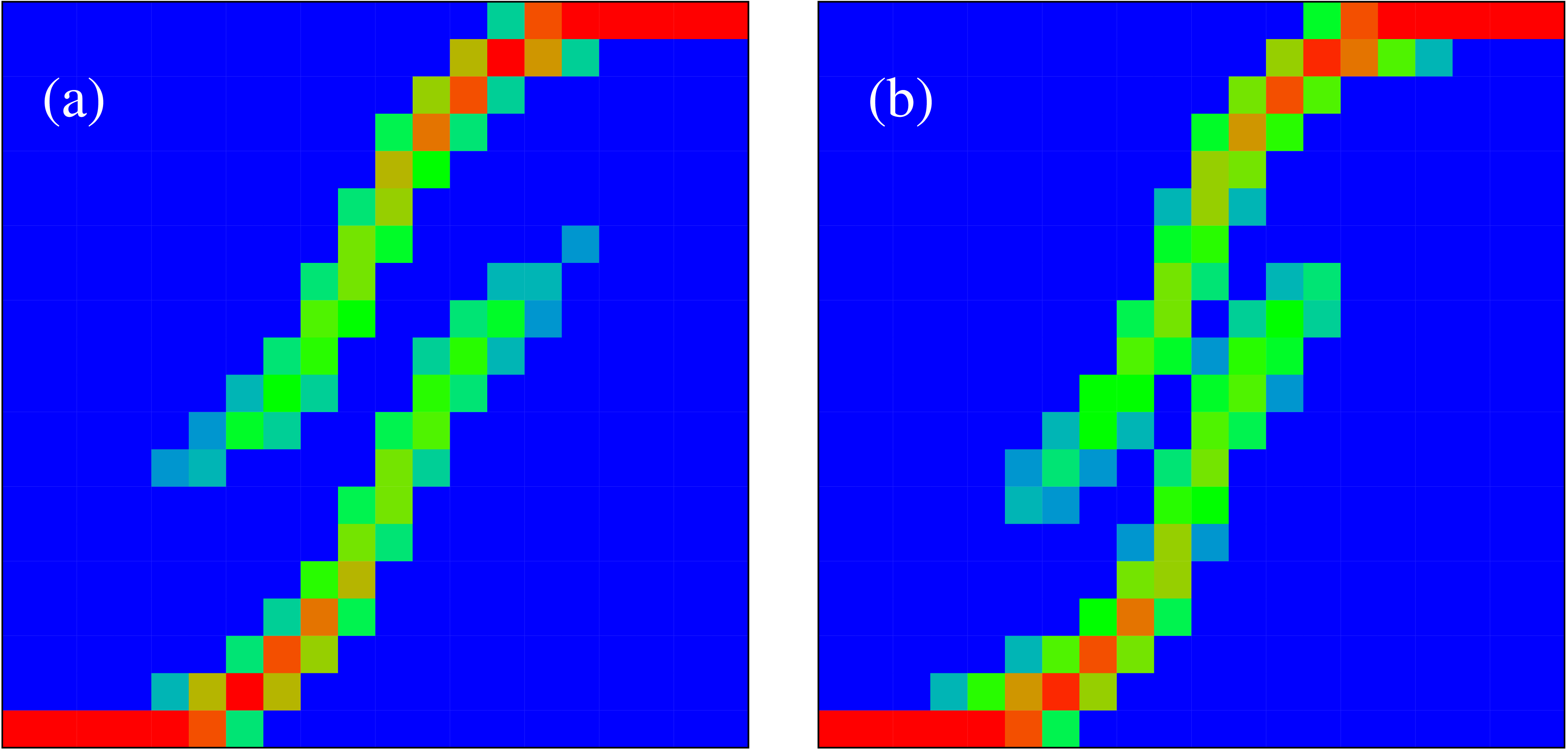
The main part of studies is done for the WWW of Cambridge and Oxford discussed above. We start with a random realization of a given fraction of red nodes $f_{i}=f(t=0)$ which evolution in time converges to a steady state with a final fraction of red nodes $f_{f}$ approximated after time $t_{c}\approx 10$. However, different initial realisations with the same $f_{i}$ value evolve to different final fractions $f_{f}$ clearly showing a bistability phenomenon. To analyze how the final fraction of red nodes $f_{f}$ depends on its initial fraction $f_{i}$, we study the time evolution $f(t)$ for a large number $N_{r}$ of initial random realizations of colors following it up to the convergence time for each realization. We find that the final red nodes are homogeneously distributed in PageRank index $K$. Thus there is no specific preference for top society levels for an initial random distribution. The probability distribution $W_{f}$ of final fractions $f_{f}$ is shown in Fig. 57 as a function of initial fraction $f_{i}$ at $a=0.1$. The results show two main features of the model: a small fraction of red opinion is completely suppressed if $f_{i}<f_{c}$ and its larger fraction dominates completely for $f_{i}>1-f_{c}$; there is a bistability phase for the initial opinion range $f_{b}\leq f_{i}\leq 1-f_{b}$. Of course, there is a symmetry in respect to exchange of red and blue colors. For the small value $a=0.1$ we have $f_{b}\approx f_{c}$ with $f_{c}\approx 0.25$. For the larger value $a=0.9$ we have $f_{c}\approx 0.35$, $f_{b}\approx 0.45$ Kandiah and Shepelyansky (2012).

Figure 58: (Color online) PROF-Sznajd model, option 1: density plot of probability $W_{f}$ to find a final red fraction $f_{f}$, shown in $y-$axis, in dependence on an initial red fraction $f_{i}$, shown in $x-$ axis; data are shown inside the unit square $0\leq f_{i},f_{f}\leq 1$. The values of $W_{f}$ are defined as a relative number of realizations found inside each of $100\times 100$ cells which cover the whole unit square. Here $N_{r}=10^{4}$ realizations of randomly distributed colors are used to obtained $W_{f}$ values; for each realization the time evolution is followed up the convergence time with up to $\tau=10^{7}$ steps. (a) Cambridge network; (b) Oxford network; here $N_{g}=8$. The probability $W_{f}$ is proportional to color changing from zero (blue/black) to unity (red/gray). After Kandiah and Shepelyansky (2012).

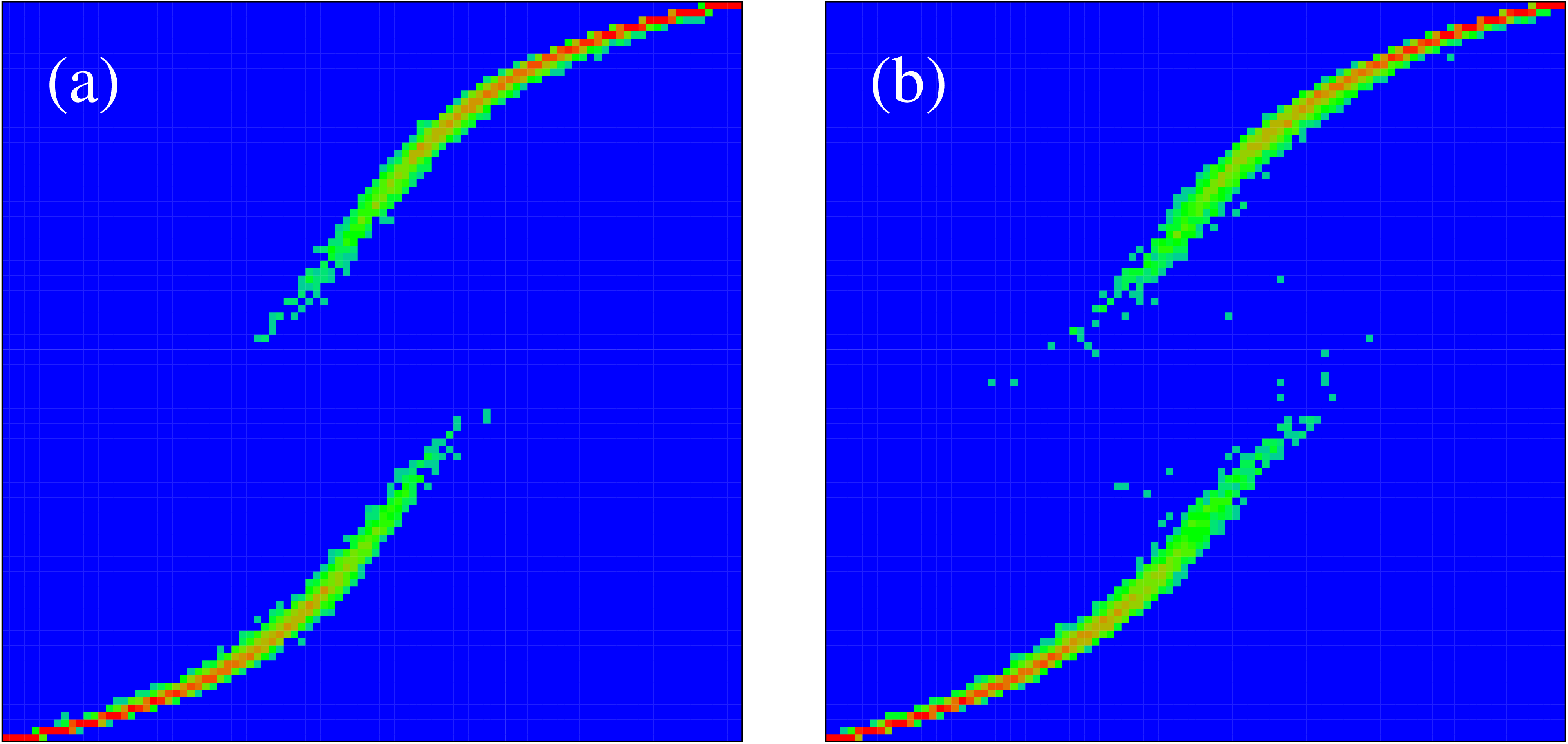
Our interpretation of these results is the following. For small values of $a\ll 1$ the opinion of a given society member is determined mainly by the PageRank of neighbors to whom he/she points (outgoing links). The PageRank probability $P$ of nodes to which many nodes point is usually high, since $P$ is proportional to the number of ingoing links. Thus at $a\ll 1$ the society is composed of members who form their opinion by listening to an elite opinion. In such a society its elite with one color opinion can impose this opinion on a large fraction of the society. Indeed, the direct analysis of the case, where the top $N_{top}=2000$ nodes of PageRank index have the same red color, shows that this 1% of the society elite can impose its opinion to about 50% of the whole society at small $a$ values (conformist society) while at large $a$ values (tenacious society) this fraction drops significantly (see Fig.4 in Kandiah and Shepelyansky (2012)). We attribute this to the fact that in Fig. 57 we start with a randomly distributed opinion, since the opinion of the elite has two fractions of two colors this creates a bistable situation when the two fractions of society follow the opinions of this divided elite, which makes the situation bistable on a larger interval of $f_{i}$ compared to the case of a tenacious society at $a\rightarrow 1$. When we replace in (17) $P$ by $1$ then the bistability disappears.

However, the detailed understanding of the opinion formation on directed networks still waits it development. Indeed, the results of PROF model for the LiveJournal and Twitted networks show that the bistability in these networks practically disappears. Also e.g. for the Twitter network studied in Sec. X.1, the elite of $N_{top}=35000$ (about 0.1% of the whole society) can impose its opinion to 80% of the society at small $a<0.15$ and to about 30% for $a>0.15$ Kandiah and Shepelyansky (2012). It is possible that a large number of links between top PageRank nodes in Twitter creates a stronger tendency to a totalitarian opinion formation comparing to the case of University networks. At the same time the studies of opinion formation with the PROF model on the Ulam networks Chakhmakhchyan and Shepelyansky (2013), which have not very large number of links, show practically no bistability in opinion formation. It is expected that a small number of loops is at the origin of such a difference in respect to university networks.

Finally we discuss a more generic version of opinion formation called the PROF-Sznajd model Kandiah and Shepelyansky (2012). Indeed, we see that in the PROF model on university network opinions of small groups of red nodes with $f_{i}<f_{c}$ are completely suppressed that seems to be not very realistic. In fact, the Sznajd model Sznajd-Weron and Sznajd (2000) features the idea of resistant groups of a society and thus incorporates a well-known trade union principle “United we stand, divided we fall”. Usually the Sznajd model is studied on regular lattices. Its generalization for directed networks is done on the basis of the notion of group of nodes $N_{g}$ at each discrete time step $\tau$.

The evolution of group is defined by the following rules:

$(a)$ we pick in the network by random a node $i$ and consider the polarization of $N_{g}-1$ highest PageRank nodes pointing to it;

$(b)$ if node $i$ and all other $N_{g}-1$ nodes have the same color (same polarization), then these $N_{g}$ nodes form a group whose effective PageRank value is the sum of all the member values $P_{g}=\sum_{j=1}^{N_{g}}P_{j}$;

$(c)$ consider all the nodes pointing to any member of the group and check all these nodes $n$ directly linked to the group: if an individual node PageRank value $P_{n}$ is less than the defined above $P_{g}$ , the node joins the group by taking the same color (polarization) as the group nodes and increase $P_{g}$ by the value of $P_{n}$; if it is not the case, a node is left unchanged.

The above time step is repeated many times during time $\tau$, counting the number of steps and choosing a random node $i$ on each next step.

The time evolution of this PROF-Sznajd model converges to a steady state approximately after $\tau\approx 10N$ steps. This is compatible with the results obtained for the PROF model. However, the statistical fluctuations in the steady-state regime are present keeping the color distribution only on average. The dependence of the final fraction of red nodes $f_{f}$ on its initial value $f_{i}$ is shown by the density plot of probability $W_{f}$ in Fig. 58 for the university networks. The probability $W_{f}$ is obtained from many initial random realizations in a similar way to the case of Fig. 57. We see that there is a significant difference compared to the PROF model: now even at small values of $f_{i}$ we find small but finite values of $f_{f}$, while in the PROF model the red color disappears at $f_{i}<f_{c}$. This feature is related to the essence of the Sznajd model: here, even small groups can resist against the totalitarian opinion. Other features of Fig. 58 are similar to those found for the PROF model: we again observe bistability of opinion formation. The number of nodes $N_{g}$, which form the group, does not significantly affect the distribution $W_{f}$ (for studied $3\leq N_{g}\leq 13$).

The above studies of opinion formation models on scale-free networks show that the society elite, corresponding to the top PageRank nodes, can impose its opinion on a significant fraction of the society. However, for a homogeneous distribution of two opinions, there exists a bistability range of opinions which depends on a conformist parameter characterizing the opinion formation. The proposed PROF-Sznajd model shows that totalitarian opinions can be escaped from by small subcommunities. The enormous development of social networks in the last few years definitely shows that the analysis of opinion formation on such networks requires further investigations.

XV Discussion

Above we considered many examples of real directed networks where the Google matrix analysis finds useful applications. The examples belong to various sciences varying from WWW, social and Wikipedia networks, software architecture to world trade, games, DNA sequences and Ulam networks. It is clear that the concept of Markov chains and Google matrix represents now the mathematical foundation of directed network analysis.

For Hermitian and unitary matrices there are now many universal concepts, developed in theoretical physics, so that the main properties of such matrices are well understood. Indeed, such characteristics as level spacing statistics, localization and delocalization properties of eigenstates, Anderson transition Anderson (1958), quantum chaos features can be now well handled by various theoretical methods (see e.g. Akemann et al. (2011); Evers and Mirlin (2008); Guhr et al. (1998); Haake (2010); Mehta (2004)). A number of generic models has been developed in this area allowing to understand the main effects via numerical simulations and analytical tools.

In contrast to the above case of Hermitian or unitary matrices, the studies of matrices of Markov chains of directed networks are now only at their initial stage. In this review, on examples of real networks we illustrated certain typical properties of such matrices. Among them there is the fractal Weyl law, which has certain traces in the field of quantum chaotic scattering, but the main part of features are new ones. In fact, the spectral properties of Markov chains had not been investigated on a large scale. We try here to provide an introduction to the properties of such matrices which contain all information about large scale directed networks. The Google matrix is like The Library of Babel Borges (1962), which contains everything. Unfortunately, we are still not able to find generic Markov matrix models which reproduce the main features of the real networks. Among them there is the possible spectral degeneracy at damping $\alpha=1$, absence of spectral gap, algebraic decay of eigenvectors. Due to absence of such generic models it is still difficult to capture the main properties of real directed networks and to understand or predict their variations with a change of network parameters. At the moment the main part of real networks have an algebraic decay of PageRank vector with an exponent $\beta\approx 0.5-1$. However, certain examples of Ulam networks (see Figs. 13, 14) show that a delocalization of PageRank probability over the whole network can take place. Such a phenomenon looks to be similar to the Anderson transition for electrons in disordered solids. It is clear that if an Anderson delocalization of PageRank would took place, as a result of further developments of the WWW, the search engines based on the PageRank would loose their efficiency since the ranking would become very sensitive to various fluctuations. In a sense the whole world would go blind the day such a delocalization takes place. Due to that a better understanding of the fundamental properties of Google matrices and their dependencies on various system parameters have a high practical significance. We believe that the theoretical research in this direction should be actively continued. In many respects, as the Library of Babel, the Google matrix still keeps its secrets to be discovered by researchers from various fields of science. We hope that a further research will allow “to formulate a general theory of the Library and solve satisfactorily the problem which no conjecture had deciphered: the formless and chaotic nature of almost all the books.” Borges (1962)

XVI Acknowledgments

We are grateful to our colleagues M. Abel, A. D. Chepeliankii, Y.-H. Eom, B. Georgeot, O. Giraud, V. Kandiah, O. V. Zhirov for fruitful collaborations on the topics included in this review. We also thank our partners of the EC FET Open project NADINE A. Benczúr, N. Litvak, S. Vigna and colleague A.Kaltenbrunner for illuminating discussions. Our special thanks go to Debora Donato for her insights at our initial stage of this research.

Our research presented here is supported in part by the EC FET Open project “New tools and algorithms for directed network analysis” (NADINE $No$ 288956). This work was granted access to the HPC resources of CALMIP (Toulouse) under the allocation 2012-P0110. We also thank the United Nations Statistics Division for provided help and friendly access to the UN COMTRADE database.

References

- Abel and Shepelyansky (2011) Abel, M. W., and D. L. Shepelyansky, 2011, Eur. Phys. J. B 84, 493.
- Akemann et al. (2011) Akemann, G., J. Baik, and Ph. Di Francesco, 2011, The Oxford Handbook of Random Matrix Theory (Oxford University Press, Oxford).
- Albert and Barabási (2000) Albert, R., and A.-L. Barabási, 2000, Phys. Rev. Lett. 85, 5234.
- Albert and Barabási (2002) Albert, R., and A.-L. Barabási, 2002, Rev. Mod. Phys. 74, 47.
-
Alon (2014)
Alon, U.,
2014,
U.Alon web site
http://wws.weizmann.ac.il/mcb/UriAlon/ . - Altun et al. (2012) Altun, Z.F., L.A. Herndon, C. Crocker, R. Lints, and D.H. Hall (Eds.), 2012, WormAtlas http://www.wormatlas.org.
- Anderson (1958) Anderson, P. W., 1958, Phys. Rev. 109, 1492.
- Aragón et al. (2012) Aragón, P., D. Laniado, A. Kaltenbrunner, and Y. Volkovich, 2012, Proc. 8th WikiSym2012, ACM, New York 19, arXiv:1204.3799v2[cs.SI].
- Arnoldi (1951) Arnoldi, W. E., 1951, Quart. Appl. Math. 9, 17.
- Barigozzi et al. (2010) Barigozzi M. , G. Fagiolo, and D. Garlaschelli, 2010, Phys. Rev. E 81, 046104.
- Bascompte et al. (2003) Bascompte, J., P. Jordano, C.J. Melian, and J.M. Olesen, 2003, Proc. Nat. Acad. Sci. USA 100, 9383.
- Bastolla et al. (2009) Bastolla, U., M. A. Pascual-Garcia, A. Ferrera, B. Luque, and J. Bascompte, 2009, Nature (London) 458, 1018.
- Blank et al. (2002) Blank, M., G. Keller, and J. Liverani, 2002, Nonlinearity 15, 1905.
- Bohigas et al. (1984) Bohigas, O., M.-J.. Giannoni, and C. Schmit, 1984, Phys. Rev. Lett. 52, 1.
- Borges (1962) Borges, J.L., 1962, The Library of Babel (Ficciones) (Grove Press, N.Y.).
- Brin and Page (1998) Brin, S., and L. Page, 1998, Comp. Networks ISDN Syst. 30, 107.
- Brin and Stuck (2002) Brin, M., and G. Stuck, 2002, Introduction to Dynamical Systems (Cambridge University Press, Cambridge UK).
- Bruzda et al. (2010) Bruzda, W., M. Smaczyński, V. Cappellini, H.-J. Sommers, and K. Zyczkowski, 2010, Phys. Rev. E 81, 066209.
- Bullmore and Sporns (2009) Bullmore, E., and O. Sporns, 2009, Nat. Rev. Neurosci. 10, 312.
- Burgos et al. (2007) Burgos, E., H. Ceva, R.P.J. Perazzo, M. Devoto, D. Medan, M. Zimmermann,and A.M. Delbue, 2007, J. Theor. Biol. 249, 307.
- Burgos et al. (2008) Burgos, E., H. Ceva, L. Hernández, R.P.J. Perazzo, M. Devoto, and D. Medan, 2008, Phys. Rev. E 78, 046113.
- Caldarelli (2003) Caldarelli, G., 2003, Scale-free networks (Oxford Univ. Press, Oxford).
- Capocci et al. (2006) Capocci, A., V. D. P. Servedio, F. Colaiori, L. S. Buriol, D. Donato, S. Leonardi, and G. Caldarelli, 2006, Phys. Rev. E 74, 036116.
- Castellano et al. (2009) Castellano, C., S. Fortunato, and V. Loreto, 2009, Rev. Mod. Phys. 81, 591.
- Chakhmakhchyan and Shepelyansky (2013) Chakhmakhchyan, L., and D. L. Shepelyansky, 2013, Phys. Lett. A 377, 3119.
- Chepelianskii and Shepelyansky (2001) Chepelianskii, A.D., and D. L. Shepelyansky, 2001, http://www.quantware.ups-tlse.fr/talks-posters/chepelianskii2001.pdf.
- Chepelianskii (2010) Chepelianskii, A. D., 2010, arXiv:1003.5455[cs.SE].
- Chen et al. (2014) Chen, N., N. Litvak, and M. Olvera-Cravioto, 2014, arXiv:1408.3610[math.PR].
- Chirikov (1979) Chirikov, B. V., 1979, Phys. Rep. 52, 263.
- Chirikov and Shepelyansky (2008) Chirikov, B.V., and D. Shepelyansky, 2008, Scholarpedia 3(3), 3550.
- CIA (2009) Central Intelligence Agency, 2009, The CIA Wold Factbook 2010 (Skyhorse Publ. Inc.).
- Cornfeldet al. (1982) Cornfeld, I.P., Fomin, S.V., and Y.G. Sinai 1982, Ergodic Theory (Springer, New York).
- Craig and von Peter (2010) Craig, B., and G. von Peter 2010, Interbank tiering and money center bank (Discussion paper N 12/2010, Deutsche Bundesbank)
- De Benedictis and Tajoli (2011) De Benedictis, L., and L. Tajoli, 2011, The World Economy 34, 8, 1417–1454.
- Dijkstra (1982) Dijkstra, E.W., 1982, Selected Writing on Computing: a Personal Perspective (Springer-Verlag, New York).
- Dimassi and Sjöstrand (1999) Dimassi, M., and J. Sjöstrand, 1999, Spectral Asymptotics in the Semicalssical Limit (Cambridge University Press, Cambridge)
- Donato et al. (2004) Donato, D., L. Laura, S. Leonardi, and S. Millozzi, 2004, Eur. Phys. J. B 38, 239.
- Dorogovtsev et al. (2008) Dorogovtsev, S. N., A. V. Goltsev, and J. F. F. Mendes, 2008, Rev. Mod. Phys. 80, 1275.
- Dorogovtsev (2010) Dorogovtsev, S., 2010, Lectures on Complex Networks (Oxford University Press, Oxford).
- Ensemble Genome database (2011) Ensemble Genome database, 2011, Ensemble Genome database http://www.ensembl.org/ .
- Eom and Shepelyansky (2013a) Eom, Y.-H., and D. L. Shepelyansky, 2013a, PLoS ONE 8(10), e74554.
- Eom et al. (2013b) Eom, Y.-H., K. M. Frahm, A. Benczúr, and D. L. Shepelyansky, 2013b, Eur. Phys. J. B 86, 492.
- Eom et al. (2014) Eom, Y.-H., P. Aragón, D. Laniado, A. Kaltenbrunner, S. Vigna, and D. L. Shepelyansky, 2014, arXiv:1405.7183 [cs.SI] (submitted to PLoS ONE).
- Ermann and Shepelyansky (2010a) Ermann, L., and D. L. Shepelyansky, 2010a, Phys. Rev. E 81, 036221.
- Ermann and Shepelyansky (2010b) Ermann, L., and D. L. Shepelyansky, 2010b, Eur. Phys. J. B 75, 299.
- Ermann et al. (2011a) Ermann, L., A. D. Chepelianskii, and D. L. Shepelyansky, 2011a, Eur. Phys. J. B 79, 115.
- Ermann and Shepelyansky (2011b) Ermann, L., and D. L. Shepelyansky, 2011b, Acta Phys. Polonica A 120(6A), A158; http://www.quantware.ups-tlse.fr/QWLIB/tradecheirank/.
- Ermann et al. (2012a) Ermann, L., A. D. Chepelianskii, and D. L. Shepelyansky, 2012a, J. Phys. A: Math. Theor. 45, 275101; http://www.quantware.ups-tlse.fr/QWLIB/dvvadi/.
- Ermann and Shepelyansky (2012b) Ermann, L., and D. L. Shepelyansky, 2012b, Physica D 241, 514.
- Ermann and Shepelyansky (2013a) Ermann, L., and D. L. Shepelyansky, 2013a, Phys. Lett. A 377, 250.
- Ermann et al. (2013b) Ermann, L., K. M. Frahm, and D. L. Shepelyansky, 2013b, Eur. Phys. J. B 86, 193.
- Ermann and Shepelyansky (2015) Ermann, L., and D. L. Shepelyansky, 2015, Eur. Phys. J. B 88, 84.
- Evers and Mirlin (2008) Evers, F., and A. D. Mirlin, 2008, Rev. Mod. Phys. 80, 1355.
- Felleman and van Essen (1991) Felleman, D.J., and D. C. van Essen, 1991, Celeb. Cortex 1, 1.
FETNADINE database (2014)
FETNADINE database,
2014, Quantware group, http://
www.quantware.ups-tlse.fr/FETNADINE/datasets.htm - Fogaras (2003) Fogaras, D., 2003, Lect. Not. Comp. Sci. 2877, 65.
- Fortunato (2010) Fortunato, S., 2010, Phys. Rep. 486, 75.
- Frahm and Shepelyansky (2009) Frahm, K. M., and D. L. Shepelyansky, 2009, Phys. Rev. E 80, 016210 .
- Frahm and Shepelyansky (2010) Frahm, K. M., and D. L. Shepelyansky, 2010, Eur. Phys. J. B 76, 57.
- Frahm et al. (2011) Frahm, K. M., B. Georgeot, and D. L. Shepelyansky, 2011, J. Phys A: Math. Theor. 44, 465101.
- Frahm et al. (2012a) Frahm, K. M., A. D. Chepelianskii, and D. L. Shepelyansky, 2012a, J. Phys A: Math. Theor. 45, 405101.
- Frahm and Shepelyansky (2012b) Frahm, K. M., and D. L. Shepelyansky, 2012b, Eur. Phys. J. B 85, 355.
- Frahm and Shepelyansky (2012c) Frahm, K. M., and D. L. Shepelyansky, 2012c, Phys. Rev. E 85, 016214.
- Frahm and Shepelyansky (2013) Frahm, K. M., and D. L. Shepelyansky, 2013, Eur. Phys. J. B 86, 322.
- Frahm and Shepelyansky (2014a) Frahm, K. M., and D. L. Shepelyansky, 2014a, Eur. Phys. J. B 87, 93.
- Frahm et al. (2014b) Frahm, K. M., Y.-H.. Eom, and D. L. Shepelyansky, 2014b, Phys. Rev. E 89, 052814.
- Franceschet (2011) Franceschet, M., 2011, Communications of the ACM 54(6), 92.
- Froyland and Padberg (2009) Froyland, G., and K. Padberg 2009, Physica D 238, 1507.
- Galam (1986) Galam, S., 1986, J. Math. Psych. 30, 426.
- Galam (2008) Galam, S., 2008, Int. J. Mod. Phys. C 19, 409.
- Gamow (1928) Gamow, G. A., 1928, Z. für Phys 51, 204.
- Gantmacher (2000) Gantmacher, F.R., 2000, The Theory of Matrices, Vol. 2 (AMS Chelsea Publ., New York).
- Garlaschelli and Loffredo (2005) Garlaschelli, D., and M. I. Loffredo 2005, Physica A: Stat. Mech. Appl. 355, 138.
- Garratt et al. (2011) Garratt, R.J., Mahadeva, L., and K. Svirydzenka, 2011, Mapping systemic risk in the international banking network (Working paper N 413, Bank of England)
- Gaspard (1998) Gaspard, P., 1998, Chaos, Scattering and Statistical Mechanics (Cambridge Univ. Press, Cambridge).
- Gaspard (2014) Gaspard, P., 2014, Scholarpedia 9(6), 9806.
- Georgeot et al. (2010) Georgeot, B., O. Giraud, and D. L. Shepelyansky, 2010, Phys. Rev. E 81, 056109.
- Georgeot and Giraud (2012) Georgeot, B., and O. Giraud, 2012, Eurphys. Lett. 97, 68002.
- Giraud et al. (2005) Giraud, O., B. Georgeot, and D. L. Shepelyansky, 2005, Phys. Rev. E 72, 036203.
- Giraud et al. (2009) Giraud, O., B. Georgeot, and D. L. Shepelyansky, 2009, Phys. Rev. E 80, 026107.
- Goldsheid and Khoruzhenko (1998) Goldsheid, I.Y., and B.A. Khoruzhenko, 1998, Phys. Rev. Lett. 80, 2897.
- Golub and Greif (2006) Golub, G. H., and C. Greif, 2006, BIT Num. Math. 46, 759.
- Guhr et al. (1998) Guhr, T., A. Mueller-Groeling, and H. A. Weidenmueller, 1998, Phys. Rep. 299, 189.
- Haake (2010) Haake, F., 2010, Quantum Signatures of Chaos (Springer-Verlag, Berlin).
- Hart (1992) Hart, M.H., 1992, The 100: ranking of the most influential persons in history (Citadel Press, N.Y.).
- He and Deem (2010) He, J. and M. W. Deem, 2010, Phys. Rev. Lett. 105, 198701.
- Hrisitidis et al. (2008) Hrisitidis, V., H. Hwang, and Y. Papakonstantinou, 2008, ACM Trans. Database Syst. 33, 1.
- Izhikevich and Edelman (2008) Izhikevich, E.M., and G. M. Edelman, 2008, Proc. Nat. Acad. Sci. 105, 3593.
- Jelenkovic and Olvera-Cravioto (2013) Jelenkovic, P.R., and M. Olvera-Cravioto, 2013, Springer Proc. Math. Statistics (Berlin, Eds. G.Alsmeyer and M. Löwe) 53, 159.
- Kandiah and Shepelyansky (2012) Kandiah, V., and D. L. Shepelyansky, 2012, Physica A 391, 5779.
- Kandiah and Shepelyansky (2013) Kandiah, V., and D. L. Shepelyansky, 2013, PLoS ONE 8(5), e61519.
- Kandiah and Shepelyansky (2014a) Kandiah, V., and D. L. Shepelyansky, 2014a, Phys. Lett. A 378, 1932.
- Kandiah et al. (2014b) Kandiah, V., B. Georgeot, and O. Giraud, 2014b, Eur. Phys. J. B 87, 246.
- Kandiah et al. (2015) Kandiah, V., H. Escaith, and D.L. Shepelyansky, 2015, arXiv:1504.06773 [q-fin.ST] .
- Kernighan and Ritchie (1978) Kernighan, B.W., and D.M. Ritchie, 1978, The C Programming Language (Englewood Cliffs, NJ Prentice Hall).
- Kleinberg (1999) Kleinberg, J.M., 1999, Jour. of the ACM 46(5), 604.
- Krapivsky et al. (2010) Krapivsky, P.L., S. Redner, and E. Ben-Naim, 2010, A Kinetic View of Statistical Physics (Cambridge University Press, Cambridge UK).
- Krugman et al. (2011) Krugman, P. R., M. Obstfeld, and M. Melitz, International economics: theory & policy, 2011, Prentic Hall, New Jersey.
- Landau and Lifshitz (1989) Landau, L.D., and E.M. Lifshitz, 1989, Quantum Mechanics (Nauka, Moscow).
- Langville and Meyer (2006) Langville, A.M., and C.D. Meyer, 2006, Google’s PageRank and Beyond: The Science of Search Engine Rankings (Princeton University Press, Princeton).
- Li (1976) Li, T.-Y., 1976, J. Approx. Theory 17, 177.
- Lichtenberg and Lieberman (1992) Lichtenberg, A. J., and M.A. Lieberman, 1992, Regular and Chaotic Dynamics (Springer, Berlin).
- Linux (2010) Linux Kernel releases are downloaded from, 2010, http://www.kernel.org/ .
- Litvak et al. (2008) Litvak, N., W. R. W. Scheinhardt, and Y. Volkovich, 2008, Lect. Not. Comp. Sci. (Springer) 4936, 72.
- Lu et al. (2003) Lu, W.T., S. Sridhar, and M. Zworski, 2003, Phys. Rev. Lett. 91, 154101.
- Mantegna et al. (1995) Mantegna, R.N., S.V. Buldyrev, A.L. Goldberger, S. Havlin, C.-K. Peng, M. Simons, and H.E. Stanley, 1995, Phys. Rev. E 52, 2939.
- Markov (1906) Markov, A. A., 1906, Izvestiya Fiziko- matematicheskogo obschestva pri Kazanskom universitete, 2-ya seriya (in Russian) 15, 135.
- May (2001) May, R.M., 2001, Stability and Complexity in Model Ecosystems (Princeton Univ. Press, New Jersey, USA).
- Mehta (2004) Mehta, M. L., 2004, Random matrices (Elsevier-Academic Press, Amsterdam).
- Memmott et al. (2004) Memmott, J., N.M. Waser, and M.V. Price, 2004, Proc. R. Soc. Lond. B 271, 2605.
- Meusel et al. (2014) Meusel, R., S. Vigna, O. Lehmberg, and C. Bizer, 2014, Proc. WWW’14 Companion, http://dx.doi.org/10.1145/2567948.2576928.
- Milo et al. (2002) Milo, R., S. Shen-Orr, S. Itzkovitz, N. Kashtan, D. Chklovskii, and U. Alon, 2002, Science 298, 824.
- Muchnik et al. (2007) Muchnik, L., R. Itzhack, S. Solomon, and Y. Louzoun, 2007, Phys. Rev. E 76, 016106.
- von Neumann (1958) von Neumann, J., 1958, The Computer and The Brain (Yale Univ. Press, New Haven CT).
- Newman (2001) Newman, M. E. J., 2001, Proc. Natl. Acad. Sci. USA 98, 404.
- Newman (2003) Newman, M. E. J., 2003, SIAM Review 45, 167.
- Newman (2010) Newman, M. E. J., 2010, Networks: An Introduction (Oxford University Press, Oxford UK).
- Nonnenmacher and Zworski (2007) Nonnenmacher, S., and M. Zworski, 2007, Commun. Math. Phys. 269, 311.
- Nonnenmacher et al. (2014) Nonnenmacher, S., J. Sjoestrand, and M. Zworski, 2014, Ann. Math. 179, 179.
- Olesen et al. (2007) Olesen, J.M., J. Bascompte, Y.L. Dupont, and P. Jordano, 2007, Proc. Natl. Acad. Sci. USA 104, 19891.
- Pandurangan et al. (2005) Pandurangan, G., P. Raghavan, and E. Upfal, 2005, Internet Math. 3, 1.
- Pantheon MIT project (2014) Pantheon MIT project, 2014, Pantheon MIT project http://pantheon.media.mit.edu .
- Perra et al. (2009) Perra, N., V. Zlatic, A. Chessa, C. Conti, D. Donato, and G. Caldarelli, 2009, Europhys. Lett. 88, 48002.
- Radicchi et al. (2009) Radicchi, F., S. Fortunato, B. Markines, and A. Vespignani, 2009, Phys. Rev. E 80, 056103.
- Redner (1998) Redner, S., 1998, Eur. Phys. J. B 4, 131.
- Redner (2005) Redner, S., 2005, Phys. Today 58(6), 49.
- Rezende et al. (2007) Rezende, E.L., J.E. Lavabre, P.R. Guimaraes, P. Jordano, and J. Bascompte, 2007, Nature (London) 448, 925.
- Rodríguez-Gironés et al. (2006) Rodríguez-Gironés, M.A., and L. Santamaría, 2006, J. Biogeogr. 33, 924.
- Saverda et al. (2011) Saverda, S., D.B. Stouffer, B. Uzzi, and J. Bascompte, 2011, Nature (London) 478, 233.
- Serra-Capizzano (2005) Serra-Capizzano, S., 2005, SIAM J. Matrix Anal. Appl. 27, 305.
- Serrano et al. (2007) Serrano, M. A., M. Boguna, and A. Vespignani, 2007, J. Econ. Interac. Coor. 2, 111.
- Shanghai ranking (2010) Shanghai ranking, 2010, Academic ranking of world universities http://www.shanghairanking.com/ .
- Shen-Orr et al. (2002) Shen-Orr, A., R. Milo, S. Mangan, and U. Alon, 2002, Nature Genetics 31(1), 64.
- Shepelyansky (2001) Shepelyansky, D. L., 2001, Phys. Scripta T90, 112.
- Shepelyansky (2008) Shepelyansky, D. L., 2008, Phys. Rev. E 77, 015202(R).
- Shepelyansky and Zhirov (2010a) Shepelyansky, D. L., and O. V. Zhirov, 2010a, Phys. Rev. E 81, 036213.
- Shepelyansky and Zhirov (2010b) Shepelyansky, D. L., and O. V. Zhirov, 2010b, Phys. Lett. A 374, 3206.
- Sjöstrand (1990) Sjöstrand, J., 1990, Duke Math. J. 60, 1.
- SJR (2007) SJR, 2007, SCImago. (2007). SJR SCImago Journal & Country Rank http://www.scimagojr.com .
- Skiena and Ward (2014) Skiena, S., and C.B. Ward, 2014, Who’s bigger?: where historical figures really rank (Cambridge University Press, New York); http://www.whoisbigger.com/.
- Soramaki et al. (2007) Soramäki, K., M. L. Bech, J. Arnold, R. J. Glass, and W. E. Beyeler, 2005, Physica A 379, 317.
- Song et al. (2005) Song, C., S. Havlin, and H.A. Makse, 2005, Nature (London) 433, 392.
- Sporns (2007) Sporns, O., 2007, Scholarpedia 2(10), 4695.
- Stewart (2001) Stewart, G. W., 2001, Matrix Algorithms Vol. II: Eigensystems (SIAM, Philadelphia PA).
- Sznajd-Weron and Sznajd (2000) Sznajd-Weron, K., and J. Sznajd, 2000, Int. J. Mod. Phys. C 11, 1157.
- Towlson et al. (2013) Towlson, E.K., P. E. Vértes, S.E. Ahnert, W.R. Schafer, and E.T. Bullmore, 2013, J. Neurosci. 33(15), 6380.
- Tromp and Farnebäck (2007) Tromp, J., and G. Farnebäck, 2007, Lect. Notes Comp. Sci. (Springer) 4630, 84.
- UK universities (2011) UK universities, 2011, Academic Web Link Database http://cybermetrics.wlv.ac.uk/database/ .
- Ulam (1960) Ulam, S., 1960, A Collection of Mathematical Problems (Interscience Tracs in Pure and Applied Mathematics, Interscience, New York).
- UN COMTRADE (2011) UN COMTRADE, 2011, United Nations Commodity Trade Statistics Database http://comtrade.un.org/db/ .
- Vázquez and Aizen (2004) Vázquez, D.P., and M. A. Aizen, 2004, Ecology 85, 1251.
- Vigna (2013) Vigna, S., 2013, arXiv:0912.0238v13[cs.IR] .
- Watts and Strogatz (1998) Watts, D. J., and S. H. Strogatz, 1998, Nature (London) 393, 440.
- Weyl (1912) Weyl, H., 1912, Math. Ann. 141, 441.
- Wikipedia Top 100 (2014) Wikipedia top 100 article, 2014, Top 100 historical figures of Wikipedia http://www.wikipedia.org/en
- Zaller (1999) Zaller, J.R., 1999, The Nature and Origins of Mass Opinion (Cambridge University Press, Cambridge UK).
- Zhirov et al. (2010) Zhirov, A. O., O. V. Zhirov, and D. L. Shepelyansky, 2010, Eur. Phys. J. B 77, 523; http://www.quantware.ups-tlse.fr/QWLIB/2drankwikipedia/ .
- Zhirov and Shepelyansky (2015) Zhirov, O. V., and D. L. Shepelyansky, 2015, Ann. Phys. (Berlin) XX, DOI 10.1002/andp.201500110.
- Zipf (1949) Zipf, G. K., 1949, Human Behavior and the Principle of Least Effort (Addison-Wesley, Boston).
- Zlatic et al. (2006) Zlatic, V., M. Bozicevic, H. Stefancic, and M. Domazet, 2006, Phys. Rev. E 74, 016115.
- Zuo et al. (2012) Zuo, X.-N., R. Ehmke, M. Mennes, D. Imperati, F.X. Castellanos, O. Sporns, and M.P. Milham, 2012, Cereb. Cortex 22, 1862.
- Zworski (1999) Zworski, M., 1999, Not. Am. Math. Soc. 46, 319.
- Zyczkowski et al. (2003) Zyczkowski, K., M. Kus, W. Slomczynski, and H.-J. Sommers, 2003, J. Phys. A: Math. Gen. 36, 3425.