Singularity free analysis of a self-similar model of proton structure function at small x

Baishali Saikia1,a and D. K. Choudhury1,2
1Department of Physics,Β Gauhati University, Guwahati-781 014, India.
2 Physics Academy of North-East, Guwahati-781014, India.
aemail: baishalipiks@gmail.com
Abstract

In this paper we make re-analysis of a self-similarity based model of the proton structure function at small x pursued in recent years. The additional assumption is that it should be singularity free in the entire kinematic range 0<x<10x10<\textit{x}<1. Our analysis indicates that the model is valid in a more restrictive range of Q2superscript𝑄2Q^{2}. We also discuss the possibility of incorporation of Froissart saturation condition in the model.

Keywords: Self-similarity, quark, gluon.
PACS Nos. :05.45.Df, Β 24.85.+p

1 Introduction

Self-similarity is a possible feature of multi-partons inside a proton at small x suggested by Lastovicka [1] and pursued by us in recent years [2, 3, 4, 5, 6]. More recently, we have examined its consequences in [7] double parton distribution function(dPDF) to be tested at LHC, in Froissart saturation [8] and Longitudinal structure function [9].

One of the theoretical limitations of the model of Ref [1] is that it has a singularity at x∼1.172Γ—10βˆ’4similar-toπ‘₯1.172superscript104x\sim 1.172\times 10^{-4} which is within the physically allowed range 0<x<10π‘₯10<x<1. Even though outside its phenomenological range of validity 6.2Γ—10βˆ’7<x<0.016.2superscript107π‘₯0.016.2\times 10^{-7}<x<0.01, such singularity is beyond common expectations from any physically viable model of proton structure function F2​(x,Q2)subscript𝐹2π‘₯superscript𝑄2F_{2}(x,Q^{2}).

In the present paper, we therefore make a re-analysis of the model of Ref[1], demanding it to be singularity free in the entire xπ‘₯x-range of 0<x<10π‘₯10<x<1.

Present work will also study the consequences of the suggestion of Ref[8] in the context of the reported reanalysis. In section2, we outline the formalism and in section3, we discuss the results. Section4 contains the conclusions.

2 Formalism

2.1 Proton Structure Function based on self-similarity

The self-similarity based model of the proton structure function of Ref[1] is based on transverse momentum dependent parton distribution function(TMD) fi​(x,kt2)subscript𝑓𝑖π‘₯superscriptsubscriptπ‘˜π‘‘2f_{i}(x,k_{t}^{2}). Here kt2superscriptsubscriptk𝑑2\textit{k}_{t}^{2} is the parton transverse momentum squared. Choosing the magnification factors (1x)1π‘₯\left(\frac{1}{x}\right) and (1+kt2Q02)1superscriptsubscriptπ‘˜π‘‘2superscriptsubscript𝑄02\left(1+\frac{k_{t}^{2}}{Q_{0}^{2}}\right), it is written as [1, 7, 8]

log[M2.fi(x,kt2)]=D1.log1x.log(1+kt2Q02)+D2.log1x+D3.log(1+kt2Q02)+D0ilog[M^{2}.f_{i}(x,k_{t}^{2})]=D_{1}.log\frac{1}{x}.log\left(1+\frac{k_{t}^{2}}{Q_{0}^{2}}\right)+D_{2}.log\frac{1}{x}+D_{3}.log\left(1+\frac{k_{t}^{2}}{Q_{0}^{2}}\right)+D_{0}^{i} (1)

where i denotes a quark flavor. Here D1,D2,D3subscript𝐷1subscript𝐷2subscript𝐷3D_{1},\ D_{2},\ D_{3} are the three flavor independent model parameters while D0isuperscriptsubscript𝐷0𝑖D_{0}^{i} is the only flavor dependent normalization constant. M2(=1 GeV2) is introduced to make (PDF) qi​(x,Q2)subscriptπ‘žπ‘–π‘₯superscript𝑄2q_{i}(x,Q^{2}) as defined below (in Eqn(2)) dimensionless. The integral quark densities then defined as:

qi​(x,Q2)=∫0Q2fi​(x,kt2)​𝑑kt2subscriptπ‘žπ‘–π‘₯superscript𝑄2superscriptsubscript0superscript𝑄2subscript𝑓𝑖π‘₯superscriptsubscriptπ‘˜π‘‘2differential-dsuperscriptsubscriptπ‘˜π‘‘2q_{i}(x,Q^{2})=\int_{0}^{Q^{2}}f_{i}(x,k_{t}^{2})dk_{t}^{2} (2)

As a result, the following analytical parametrization of a quark density is obtained by using Eqn(2) [6]

qi​(x,Q2)=eD0i​f​(x,Q2)subscriptπ‘žπ‘–π‘₯superscript𝑄2superscript𝑒superscriptsubscript𝐷0𝑖𝑓π‘₯superscript𝑄2q_{i}(x,Q^{2})=e^{D_{0}^{i}}f(x,Q^{2}) (3)

where,

f​(x,Q2)=Q02​xβˆ’D2M2​(1+D3+D1​l​o​g​(1x))Γ—((1x)D1​l​o​g​(1+Q2Q02)​(1+Q2Q02)D3+1βˆ’1)𝑓π‘₯superscript𝑄2superscriptsubscript𝑄02superscriptπ‘₯subscript𝐷2superscript𝑀21subscript𝐷3subscript𝐷1π‘™π‘œπ‘”1π‘₯superscript1π‘₯subscript𝐷1π‘™π‘œπ‘”1superscript𝑄2superscriptsubscript𝑄02superscript1superscript𝑄2superscriptsubscript𝑄02subscript𝐷311f(x,Q^{2})=\frac{Q_{0}^{2}\ x^{-D_{2}}}{M^{2}\left(1+D_{3}+D_{1}log\left(\frac{1}{x}\right)\right)}\\ \times\left(\left(\frac{1}{x}\right)^{D_{1}log\left(1+\frac{Q^{2}}{Q_{0}^{2}}\right)}\left(1+\frac{Q^{2}}{Q_{0}^{2}}\right)^{D_{3}+1}-1\right) (4)

is flavor independent. Using Eqn(3) in the usual definition of the structure function F2​(x,Q2)subscript𝐹2π‘₯superscript𝑄2F_{2}(x,Q^{2}), one can get

F2​(x,Q2)=xβ€‹βˆ‘iei2​(qi​(x,Q2)+qΒ―i​(x,Q2))subscript𝐹2π‘₯superscript𝑄2π‘₯subscript𝑖superscriptsubscript𝑒𝑖2subscriptπ‘žπ‘–π‘₯superscript𝑄2subscriptΒ―π‘žπ‘–π‘₯superscript𝑄2F_{2}(x,Q^{2})=x\sum_{i}e_{i}^{2}\left(q_{i}(x,Q^{2})+\bar{q}_{i}(x,Q^{2})\right) (5)

or it can be written as

F2​(x,Q2)=eD0​x​f​(x,Q2)subscript𝐹2π‘₯superscript𝑄2superscript𝑒subscript𝐷0π‘₯𝑓π‘₯superscript𝑄2F_{2}(x,Q^{2})=e^{D_{0}}xf(x,Q^{2}) (6)

where D0=βˆ‘iD0isubscript𝐷0subscript𝑖superscriptsubscript𝐷0𝑖D_{0}=\sum_{i}D_{0}^{i}. From HERA data [10, 11], Eqn(6) was fitted with

D0subscript𝐷0\displaystyle D_{0} =\displaystyle= 0.339±0.145plus-or-minus0.3390.145\displaystyle 0.339\pm 0.145
D1subscript𝐷1\displaystyle D_{1} =\displaystyle= 0.073±0.001plus-or-minus0.0730.001\displaystyle 0.073\pm 0.001
D2subscript𝐷2\displaystyle D_{2} =\displaystyle= 1.013±0.01plus-or-minus1.0130.01\displaystyle 1.013\pm 0.01
D3subscript𝐷3\displaystyle D_{3} =\displaystyle= βˆ’1.287Β±0.01plus-or-minus1.2870.01\displaystyle-1.287\pm 0.01
Q02superscriptsubscript𝑄02\displaystyle Q_{0}^{2} =\displaystyle= 0.062Β±0.01​G​e​V2plus-or-minus0.0620.01𝐺𝑒superscript𝑉2\displaystyle 0.062\pm 0.01\ GeV^{2} (7)

in the kinematical region,

0.62Γ—10βˆ’7≀x≀10βˆ’20.62superscript107π‘₯superscript102\displaystyle 0.62\times 10^{-7}\leq x\leq 10^{-2}
0.045≀Q2≀120​G​e​V20.045superscript𝑄2120𝐺𝑒superscript𝑉2\displaystyle 0.045\leq Q^{2}\leq 120\ GeV^{2} (8)

2.2 Singularity free Structure Function

The model of Ref[1] has two inherent limitations. First, the parameter D3subscript𝐷3D_{3} is negative contrary to the expectations of positivity of the fractal dimensions [2]. Secondly, due to its negative value, Eqn(6) develops a singularity at x∽1.172Γ—10βˆ’4∽x1.172superscript104\textit{x}\backsim 1.172\times 10^{-4} [6] as it satisfies the condition 1+D3+D1​l​o​g​1x=01subscript𝐷3subscript𝐷1π‘™π‘œπ‘”1π‘₯01+D_{3}+D_{1}log\frac{1}{x}=0, contrary to the expectation of a physically viable form of Structure Function.

The model can be made singularity free under following specific conditions of the model parameters.

Case 1 : If D1,D3β‰ͺD2much-less-thansubscript𝐷1subscript𝐷3subscript𝐷2D_{1},D_{3}\ll D_{2} in Eqn(1) then the PDF Eqn(3) and the Structure Function Eqn(6) will be of the form:

qi​(x,Q2)=eD0i​Q2​xβˆ’D2M2subscriptπ‘žπ‘–π‘₯superscript𝑄2superscript𝑒superscriptsubscript𝐷0𝑖superscript𝑄2superscriptπ‘₯subscript𝐷2superscript𝑀2q_{i}(x,Q^{2})=\frac{e^{D_{0}^{i}}\ Q^{2}\ x^{-D_{2}}}{M^{2}} (9)
F2​(x,Q2)=eD0​Q2​xβˆ’D2+1M2subscript𝐹2π‘₯superscript𝑄2superscript𝑒subscript𝐷0superscript𝑄2superscriptπ‘₯subscript𝐷21superscript𝑀2F_{2}(x,Q^{2})=\frac{e^{D_{0}}\ Q^{2}\ x^{-D_{2}+1}}{M^{2}} (10)


Case 2 : In this case D1β‰ͺD2,D3much-less-thansubscript𝐷1subscript𝐷2subscript𝐷3D_{1}\ll D_{2},D_{3} in Eqn(1) then the corresponding expressions for the PDF and Structure Function in this limit are respectively:

qi​(x,Q2)=eD0i​Q02​xβˆ’D2M2​(1+D3)​((1+Q2Q02)D3+1βˆ’1)subscriptπ‘žπ‘–π‘₯superscript𝑄2superscript𝑒superscriptsubscript𝐷0𝑖superscriptsubscript𝑄02superscriptπ‘₯subscript𝐷2superscript𝑀21subscript𝐷3superscript1superscript𝑄2superscriptsubscript𝑄02subscript𝐷311q_{i}(x,Q^{2})=\frac{e^{D_{0}^{i}}\ Q_{0}^{2}\ x^{-D_{2}}}{M^{2}\left(1+D_{3}\right)}\ \left(\left(1+\frac{Q^{2}}{Q_{0}^{2}}\right)^{D_{3}+1}-1\right) (11)
F2​(x,Q2)=eD0​Q02​xβˆ’D2+1M2​(1+D3)​((1+Q2Q02)D3+1βˆ’1)subscript𝐹2π‘₯superscript𝑄2superscript𝑒subscript𝐷0superscriptsubscript𝑄02superscriptπ‘₯subscript𝐷21superscript𝑀21subscript𝐷3superscript1superscript𝑄2superscriptsubscript𝑄02subscript𝐷311F_{2}(x,Q^{2})=\frac{e^{D_{0}}\ Q_{0}^{2}\ x^{-D_{2}+1}}{M^{2}\left(1+D_{3}\right)}\ \left(\left(1+\frac{Q^{2}}{Q_{0}^{2}}\right)^{D_{3}+1}-1\right) (12)


Case 3 : In this case, D3β‰ͺD1,D2much-less-thansubscript𝐷3subscript𝐷1subscript𝐷2D_{3}\ll D_{1},D_{2} in Eqn(1) then the corresponding PDF and the Structure Function are set in the form:

qi​(x,Q2)=eD0i​Q2​xβˆ’D2M2​(1+D1​l​o​g​1x)Γ—((1x)D1​l​o​g​(1+Q2Q02)​(1+Q2Q02)βˆ’1)subscriptπ‘žπ‘–π‘₯superscript𝑄2superscript𝑒superscriptsubscript𝐷0𝑖superscript𝑄2superscriptπ‘₯subscript𝐷2superscript𝑀21subscript𝐷1π‘™π‘œπ‘”1π‘₯superscript1π‘₯subscript𝐷1π‘™π‘œπ‘”1superscript𝑄2superscriptsubscript𝑄021superscript𝑄2superscriptsubscript𝑄021q_{i}(x,Q^{2})=\frac{e^{D_{0}^{i}}\ Q^{2}\ x^{-D_{2}}}{M^{2}\left(1+D_{1}log\frac{1}{x}\right)}\\ \times\left(\left(\frac{1}{x}\right)^{D_{1}log\left(1+\frac{Q^{2}}{Q_{0}^{2}}\right)}\left(1+\frac{Q^{2}}{Q_{0}^{2}}\right)-1\right) (13)
F2​(x,Q2)=eD0​Q2​xβˆ’D2+1M2​(1+D1​l​o​g​1x)Γ—((1x)D1​l​o​g​(1+Q2Q02)​(1+Q2Q02)βˆ’1)subscript𝐹2π‘₯superscript𝑄2superscript𝑒subscript𝐷0superscript𝑄2superscriptπ‘₯subscript𝐷21superscript𝑀21subscript𝐷1π‘™π‘œπ‘”1π‘₯superscript1π‘₯subscript𝐷1π‘™π‘œπ‘”1superscript𝑄2superscriptsubscript𝑄021superscript𝑄2superscriptsubscript𝑄021F_{2}(x,Q^{2})=\frac{e^{D_{0}}\ Q^{2}\ x^{-D_{2}+1}}{M^{2}\left(1+D_{1}log\frac{1}{x}\right)}\\ \times\left(\left(\frac{1}{x}\right)^{D_{1}log\left(1+\frac{Q^{2}}{Q_{0}^{2}}\right)}\left(1+\frac{Q^{2}}{Q_{0}^{2}}\right)-1\right) (14)

respectively.

Case 4 : This is the most general case for the singularity free model, Eqn(6) under the condition that D1,D2,D3subscript𝐷1subscript𝐷2subscript𝐷3D_{1},D_{2},D_{3} are positive.

2.3 Froissart inspired Proton structure function based on self-similarity

It is to be noted that the variable in which the supposed fractal scaling in the quark distribution occur is not known for the underlying theory. In Ref[1], the choice of 1x1π‘₯\frac{1}{x} as one of the magnification factors was taken presumably because of the power law form of the quark distribution at small xπ‘₯x found in GlΓΌck-Reya-Vogt (GRV) distribution [12]. However, this form is not derived for the theory but rather inspired by the power law distribution in x assumed for GRV distribution for QCD evaluation. The choice of 1x1π‘₯\frac{1}{x} as the proper scaling variable is not an established result of the underlying theory.

A more plausible variable appears instead to be l​o​g​1xπ‘™π‘œπ‘”1π‘₯log\frac{1}{x} [13] which confirms to the Froissart saturation [14, 15] of high energy interaction.

With this choice, Transverse Momentum Dependent Structure Function (TMD) and Parton Distribution Function (PDF) now take the following forms [8]

log(M2.f~i(x,kt2))=D~1log(log(1x)).log(1+kt2Q~02)+D~2log(log(1x))+D~3log(1+kt2Q~02)+D~0ilog\left(M^{2}.\tilde{f}_{i}(x,k_{t}^{2})\right)=\tilde{D}_{1}log\left(log\left(\frac{1}{x}\right)\right).log\left(1+\frac{k_{t}^{2}}{\tilde{Q}_{0}^{2}}\right)\\ +\tilde{D}_{2}log\left(log\left(\frac{1}{x}\right)\right)+\tilde{D}_{3}log\left(1+\frac{k_{t}^{2}}{\tilde{Q}_{0}^{2}}\right)+\tilde{D}_{0}^{i} (15)

and

q~i​(x,Q2)=eD~0i​f~​(x,Q2)subscript~π‘žπ‘–π‘₯superscript𝑄2superscript𝑒superscriptsubscript~𝐷0𝑖~𝑓π‘₯superscript𝑄2\tilde{q}_{i}(x,Q^{2})=e^{\tilde{D}_{0}^{i}}\tilde{f}(x,Q^{2}) (16)

where,

f~​(x,Q2)=Q~02​xβˆ’D~2M2​(1+D~3+D~1​l​o​g​(l​o​g​(1x)))Γ—{l​o​g​(l​o​g​(1x))D~1​l​o​g​(1+Q2Q~02)​(1+Q2Q~02)D~3+1βˆ’1}~𝑓π‘₯superscript𝑄2superscriptsubscript~𝑄02superscriptπ‘₯subscript~𝐷2superscript𝑀21subscript~𝐷3subscript~𝐷1π‘™π‘œπ‘”π‘™π‘œπ‘”1π‘₯π‘™π‘œπ‘”superscriptπ‘™π‘œπ‘”1π‘₯subscript~𝐷1π‘™π‘œπ‘”1superscript𝑄2superscriptsubscript~𝑄02superscript1superscript𝑄2superscriptsubscript~𝑄02subscript~𝐷311\tilde{f}(x,Q^{2})=\frac{\tilde{Q}_{0}^{2}\ x^{-\tilde{D}_{2}}}{M^{2}\left(1+\tilde{D}_{3}+\tilde{D}_{1}log\left(log\left(\frac{1}{x}\right)\right)\right)}\\ \times\left\{log\left(log\left(\frac{1}{x}\right)\right)^{\tilde{D}_{1}log\left(1+\frac{Q^{2}}{\tilde{Q}_{0}^{2}}\right)}\left(1+\frac{Q^{2}}{\tilde{Q}_{0}^{2}}\right)^{\tilde{D}_{3}+1}-1\right\} (17)

The structure function as defined in Eqn(6) becomes

F2​(x,Q2)=eD0~​x​f~​(x,Q2)subscript𝐹2π‘₯superscript𝑄2superscript𝑒~subscript𝐷0π‘₯~𝑓π‘₯superscript𝑄2F_{2}(x,Q^{2})=e^{\tilde{D_{0}}}x\tilde{f}(x,Q^{2}) (18)

where

D0~=βˆ‘D~0i~subscript𝐷0superscriptsubscript~𝐷0𝑖\tilde{D_{0}}=\sum\tilde{D}_{0}^{i} (19)

For very small xπ‘₯x and large Q2superscript𝑄2Q^{2}, the second term of Eqn(18) can be neglected leading to

q~i​(x,Q2)=eD~0i​Q02​(l​o​g​1x)D~2+D~1​l​o​g​(1+Q2Q~02)M2​(1+D~3+D~1​l​o​g​l​o​g​(1x))​(1+Q2Q~02)D~3+1subscript~π‘žπ‘–π‘₯superscript𝑄2superscript𝑒superscriptsubscript~𝐷0𝑖superscriptsubscript𝑄02superscriptπ‘™π‘œπ‘”1π‘₯subscript~𝐷2subscript~𝐷1π‘™π‘œπ‘”1superscript𝑄2superscriptsubscript~𝑄02superscript𝑀21subscript~𝐷3subscript~𝐷1π‘™π‘œπ‘”π‘™π‘œπ‘”1π‘₯superscript1superscript𝑄2superscriptsubscript~𝑄02subscript~𝐷31\tilde{q}_{i}(x,Q^{2})=\frac{e^{\tilde{D}_{0}^{i}}Q_{0}^{2}\left(log\frac{1}{x}\right)^{\tilde{D}_{2}+\tilde{D}_{1}log\left(1+\frac{Q^{2}}{\tilde{Q}_{0}^{2}}\right)}}{M^{2}\left(1+\tilde{D}_{3}+\tilde{D}_{1}loglog\left(\frac{1}{x}\right)\right)}\left(1+\frac{Q^{2}}{\tilde{Q}_{0}^{2}}\right)^{\tilde{D}_{3}+1} (20)

which satisfies the Froissart saturation condition, if

D~2+D~1​l​o​g​(1+Q2Q02)=2subscript~𝐷2subscript~𝐷1π‘™π‘œπ‘”1superscript𝑄2superscriptsubscript𝑄022\tilde{D}_{2}+\tilde{D}_{1}log\left(1+\frac{Q^{2}}{Q_{0}^{2}}\right)=2 (21)

within l​o​g​l​o​g​(1x)π‘™π‘œπ‘”π‘™π‘œπ‘”1π‘₯loglog\left(\frac{1}{x}\right) corrections [8].

3 Results

3.1 Analysis of singularity free model

To determine the parameters of the model (D0,D1,D2,D3,Q02)subscript𝐷0subscript𝐷1subscript𝐷2subscript𝐷3superscriptsubscript𝑄02\left(D_{0},\ D_{1},\ D_{2},\ D_{3},\ Q_{0}^{2}\right) we use recently compiled HERA data [16] instead of earlier data [10, 11] used in Ref[1]. Following this procedure of Ref[1] we make Ο‡2superscriptπœ’2\chi^{2}-analysis of the data and find the following results.

Case 1 : We note that D2subscript𝐷2D_{2}=1 is ruled out since it will make the Structure Function Eqn(10) xπ‘₯x-independent. In Table 1 we show the results. From the Ο‡2superscriptπœ’2\chi^{2}-analysis, the model in case 1 is confined well with data for 0.35≀Q2≀absentsuperscript𝑄2absent\leq Q^{2}\leq70GeV2 and 6.62Γ—\times 10β‰€βˆ’6{}^{-6}\leq x ≀\leq 0.08. Note that D3subscript𝐷3D_{3} and D1subscript𝐷1D_{1} are taken to be zero in this limit. Here the number of F2subscript𝐹2F_{2} data points is 222.

Table 1: Results of the fit
D0subscript𝐷0D_{0} D1subscript𝐷1D_{1} D2subscript𝐷2D_{2} D3subscript𝐷3D_{3} Q02superscriptsubscript𝑄02Q_{0}^{2} (GeV2) Ο‡2superscriptπœ’2\chi^{2} Ο‡2/n​d​fsuperscriptπœ’2𝑛𝑑𝑓\chi^{2}/ndf
-4.129 Β±0.332plus-or-minus0.332\pm 0.332 0 1.226 Β±0.01plus-or-minus0.01\pm 0.01 0 - 180.11 0.81

Case 2 : The parameters D0,D2,D3subscript𝐷0subscript𝐷2subscript𝐷3D_{0},\ D_{2},\ D_{3} and Q02superscriptsubscript𝑄02Q_{0}^{2} are determined (given in Table 2) in the similar manner as in case 1 but the validity range is new 0.35 ≀Q2≀27absentsuperscript𝑄227\leq Q^{2}\leq 27 GeV2 and 6.62Γ—\times 10β‰€βˆ’6{}^{-6}\leq x ≀\leq 0.032. As in case 1, here too D2=1subscript𝐷21D_{2}=1 is ruled out since it will make Eqn(12) xπ‘₯x-independent. The number of F2subscript𝐹2F_{2} data points is 174.

Table 2: Results of the fit
D0subscript𝐷0D_{0} D1subscript𝐷1D_{1} D2subscript𝐷2D_{2} D3subscript𝐷3D_{3} Q02superscriptsubscript𝑄02Q_{0}^{2} (GeV2) Ο‡2superscriptπœ’2\chi^{2} Ο‡2/n​d​fsuperscriptπœ’2𝑛𝑑𝑓\chi^{2}/ndf
-6.125 Β±0.444plus-or-minus0.444\pm 0.444 0 1.214 Β±0.01plus-or-minus0.01\pm 0.01 0.531 Β±0.01plus-or-minus0.01\pm 0.01 0.053 Β±0.001plus-or-minus0.001\pm 0.001 138.67 0.80

Case 3 : Here parameters are best fitted in the range 0.35≀Q2≀absentsuperscript𝑄2absent\leq Q^{2}\leq15 GeV2 and 6.62Γ—\times 10β‰€βˆ’6{}^{-6}\leq x ≀\leq 0.02 and given in Table 3. The number of F2subscript𝐹2F_{2} data points is 146.

Table 3: Results of the fit
D0subscript𝐷0D_{0} D1subscript𝐷1D_{1} D2subscript𝐷2D_{2} D3subscript𝐷3D_{3} Q02superscriptsubscript𝑄02Q_{0}^{2} (GeV)2{}^{2}) Ο‡2superscriptπœ’2\chi^{2} Ο‡2/n​d​fsuperscriptπœ’2𝑛𝑑𝑓\chi^{2}/ndf
-3.533 Β±0.350plus-or-minus0.350\pm 0.350 0.411 Β±0.02plus-or-minus0.02\pm 0.02 0.582 Β±0.003plus-or-minus0.003\pm 0.003 0 0.035 Β±0.0005plus-or-minus0.0005\pm 0.0005 117.31 0.80

Case 4 : Parameters D0,D1,D2,D3subscript𝐷0subscript𝐷1subscript𝐷2subscript𝐷3D_{0},\ D_{1},\ D_{2},\ D_{3} and Q02superscriptsubscript𝑄02Q_{0}^{2} are determined and given in Table 4 and obtained in a more restrictive range 0.85≀Q2≀absentsuperscript𝑄2absent\leq Q^{2}\leq10 GeV2 and 2Γ—\times 10β‰€βˆ’5{}^{-5}\leq x ≀\leq0.02. The number of F2subscript𝐹2F_{2} data points is 95.

Table 4: Results of the fit
D0subscript𝐷0D_{0} D1subscript𝐷1D_{1} D2subscript𝐷2D_{2} D3subscript𝐷3D_{3} Q02superscriptsubscript𝑄02Q_{0}^{2} (GeV)2{}^{2}) Ο‡2superscriptπœ’2\chi^{2} Ο‡2/n​d​fsuperscriptπœ’2𝑛𝑑𝑓\chi^{2}/ndf
-2.971 Β±0.409plus-or-minus0.409\pm 0.409 0.065 Β±0.0003plus-or-minus0.0003\pm 0.0003 1.021 Β±0.004plus-or-minus0.004\pm 0.004 0.0003 0.20 Β±0.0008plus-or-minus0.0008\pm 0.0008 18.829 0.20

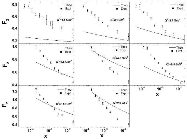
In Figure 1, we plot F2subscript𝐹2F_{2} as a function of xπ‘₯x for eight representative values of Q2superscript𝑄2Q^{2} (Q2superscript𝑄2Q^{2}= 1.5, 2, 2.7, 3.5, 4.5, 6.5, 8.5, 10 GeV2) in the phenomenological allowed range 0.85≀Q2≀absentsuperscript𝑄2absent\leq Q^{2}\leq10 GeV2. We also show the corresponding available data from Ref [16].

Our analysis indicates that the phenomenological range of validity of the present version of the model is more restrictive 0.85≀Q2≀100.85superscript𝑄2100.85\leq Q^{2}\leq 10 GeV2 and 2Γ—10βˆ’5≀x≀0.022superscript105π‘₯0.022\times 10^{-5}\leq x\leq 0.02 to be compared with Eqn(2.1) of the previous version of Ref[1].
Refer to caption
Figure 1: Measurement of the structure function F2​(x,Q2)subscript𝐹2π‘₯superscript𝑄2F_{2}(x,Q^{2}) as a function of xπ‘₯x in bins of Q2superscript𝑄2Q^{2} by recently compiled HERA data.

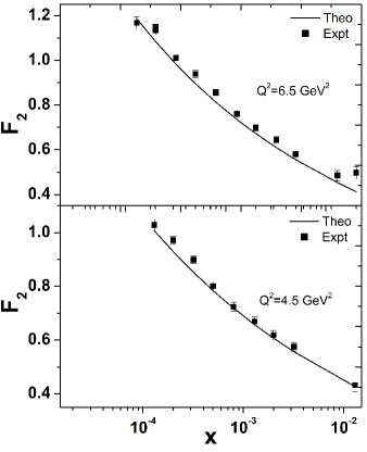
We also observe the following features of the model compared to data: at Q2=1.5superscript𝑄21.5Q^{2}=1.5GeV2 data overshoots the theory. But as Q2superscript𝑄2Q^{2} increases, the theoretical curve comes closer to data. At Q2superscript𝑄2Q^{2}=10 GeV2, on the other hand, the theory exceeds data. Main reason of this feature is that the xπ‘₯x-slope of the model is less than that of the data. This limitation can in principle be overcome by modification of the magnification factor 1x1π‘₯\frac{1}{x} to (1xβˆ’1)1π‘₯1\left(\frac{1}{x}-1\right) in Eqn(1) to accommodate proper large xπ‘₯x behavior of structure function as noted in Ref[7].

As an illustration we show results of two representative values of Q2superscript𝑄2Q^{2}= 4.5 and 6.5 GeV2 in FigureΒ 2 with such magnification using the parameters in TableΒ 4.

Refer to caption
Figure 2: Measurement of the structure function F2​(x,Q2)subscript𝐹2π‘₯superscript𝑄2F_{2}(x,Q^{2}) as a function of xπ‘₯x in bins of Q2superscript𝑄2Q^{2} by recently compiled HERA data.

3.2 Graphical representation of TMD

It is interesting to predict the kt2superscriptsubscriptπ‘˜π‘‘2k_{t}^{2}-dependance of unintegrated parton distribution (TMD) from the xπ‘₯x and Q2superscript𝑄2Q^{2} dependence of the integrated parton distribution function (PDF). Clearly this can be done within a model framework, as has been noted in Ref[17] as well as in Ref[18]. Though it should be of interest to explore this approach to study kt2superscriptsubscriptπ‘˜π‘‘2k_{t}^{2}-dependence of fi​(x,kt2)subscript𝑓𝑖π‘₯superscriptsubscriptπ‘˜π‘‘2f_{i}(x,k_{t}^{2}), such a study makes sense only in the xπ‘₯x-Q2superscript𝑄2Q^{2} range where the approach works and where the parameters had been fitted namely 2Γ—10βˆ’5≀x≀0.022superscript105π‘₯0.022\times 10^{-5}\leq x\leq 0.02 in the present model.

Using Eqn(1), fi​(x,kt2)subscript𝑓𝑖π‘₯superscriptsubscriptπ‘˜π‘‘2f_{i}(x,k_{t}^{2}) has the form

fi​(x,kt2)=eD0iM2​(1x)D2+D1​l​o​g​(1+kt2Q02)​(1+kt2Q02)D3subscript𝑓𝑖π‘₯superscriptsubscriptπ‘˜π‘‘2superscript𝑒superscriptsubscript𝐷0𝑖superscript𝑀2superscript1π‘₯subscript𝐷2subscript𝐷1π‘™π‘œπ‘”1superscriptsubscriptπ‘˜π‘‘2superscriptsubscript𝑄02superscript1superscriptsubscriptπ‘˜π‘‘2superscriptsubscript𝑄02subscript𝐷3f_{i}(x,k_{t}^{2})=\frac{e^{D_{0}^{i}}}{M^{2}}\left(\frac{1}{x}\right)^{D_{2}+D_{1}log\left(1+\frac{k_{t}^{2}}{Q_{0}^{2}}\right)}\left(1+\frac{k_{t}^{2}}{Q_{0}^{2}}\right)^{D_{3}} (22)

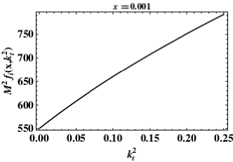
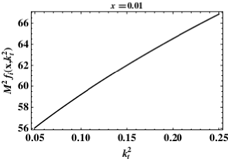
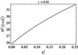
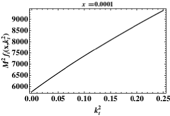
which has dimension of mass-2 consistence with Eqn(2) where the PDF qi​(x,Q2)subscriptπ‘žπ‘–π‘₯superscript𝑄2q_{i}(x,Q^{2}) is dimensionless. To evaluate Eqn(22) we take the mean value D0subscript𝐷0D_{0}, D1subscript𝐷1D_{1}, D2subscript𝐷2D_{2}, D3subscript𝐷3D_{3} and Q02superscriptsubscript𝑄02Q_{0}^{2} from the Table4. Assuming D0=nf​D0isubscript𝐷0subscript𝑛𝑓superscriptsubscript𝐷0𝑖D_{0}=n_{f}D_{0}^{i} and setting nf=4subscript𝑛𝑓4n_{f}=4, we obtain D0i=βˆ’0.742superscriptsubscript𝐷0𝑖0.742D_{0}^{i}=-0.742. In FigureΒ 3, M2​fi​(x,kt2)superscript𝑀2subscript𝑓𝑖π‘₯superscriptsubscriptπ‘˜π‘‘2M^{2}f_{i}(x,k_{t}^{2}) vs kt2superscriptsubscriptπ‘˜π‘‘2k_{t}^{2} is shown for representative values of
(i) xπ‘₯x = 10-4 (ii) xπ‘₯x = 10-3 (iii) xπ‘₯x = 10-2 (iv) xπ‘₯x=0.02 setting M2=1superscript𝑀21M^{2}=1 GeV2.

The allowed limit of kt2superscriptsubscriptπ‘˜π‘‘2k_{t}^{2} is considered to be less than the average value kt2superscriptsubscriptπ‘˜π‘‘2k_{t}^{2}=0.25 GeV2 [21] as determined from data.
Refer to caption
(a)
Refer to caption
(b)
Refer to caption
(c)
Refer to caption
(d)
Figure 3: M2​fi​(x,kt2)superscript𝑀2subscript𝑓𝑖π‘₯superscriptsubscriptπ‘˜π‘‘2M^{2}f_{i}(x,k_{t}^{2}) vs kt2superscriptsubscriptπ‘˜π‘‘2k_{t}^{2}

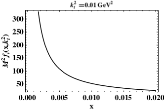
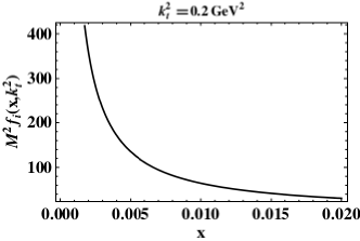
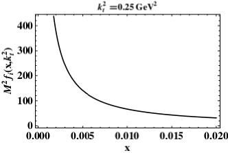
Similarly M2​fi​(x,kt2)superscript𝑀2subscript𝑓𝑖π‘₯superscriptsubscriptπ‘˜π‘‘2M^{2}f_{i}(x,k_{t}^{2}) vs xπ‘₯x as shown in FigureΒ 4 for representative values of
(i) kt2superscriptsubscriptπ‘˜π‘‘2k_{t}^{2} = 0.01 GeV2 (ii) kt2superscriptsubscriptπ‘˜π‘‘2k_{t}^{2} = 0.1 GeV2 (iii) kt2superscriptsubscriptπ‘˜π‘‘2k_{t}^{2}= Q02superscriptsubscript𝑄02Q_{0}^{2} = 0.20 GeV2 (iv) kt2superscriptsubscriptπ‘˜π‘‘2k_{t}^{2}=0.25 GeV2.

Refer to caption
(a)
Refer to caption
(b)
Refer to caption
(c)
Refer to caption
(d)
Figure 4: M2​fi​(x,kt2)superscript𝑀2subscript𝑓𝑖π‘₯superscriptsubscriptπ‘˜π‘‘2M^{2}f_{i}(x,k_{t}^{2}) vs xπ‘₯x

The present graphical analysis of TMD [FigΒ 3,4] is an improvement over the earlier one [18], in the sense that the experimental limit on kt2superscriptsubscriptπ‘˜π‘‘2k_{t}^{2} as determined from data [21] was not taken into consideration there. Further it was also beyond the range of validity of the original model. Proper dimension of the TMD has also been taken into account in the present case.

Let us now compare the structure of the model TMD (Eqn22) with the suggested forms available in current literature.

The standard way to study TMDs is through the factorization approach [20, 21, 22] where xπ‘₯x and Q2superscript𝑄2Q^{2}-dependence are factorized into a PDF qi​(x,Q2)subscriptπ‘žπ‘–π‘₯superscript𝑄2q_{i}(x,Q^{2}) and a Gaussian transverse momentum dependent function h​(kt2)β„Žsuperscriptsubscriptπ‘˜π‘‘2h(k_{t}^{2})

fi​(x,kt2,Q2)=qi​(x,Q2)​h​(kt2)subscript𝑓𝑖π‘₯superscriptsubscriptπ‘˜π‘‘2superscript𝑄2subscriptπ‘žπ‘–π‘₯superscript𝑄2β„Žsuperscriptsubscriptπ‘˜π‘‘2f_{i}(x,k_{t}^{2},Q^{2})=q_{i}(x,Q^{2})h(k_{t}^{2}) (23)

where,

h​(kt2)=1⟨kt2βŸ©β€‹eβˆ’kt2⟨kt2βŸ©β„Žsuperscriptsubscriptπ‘˜π‘‘21delimited-⟨⟩superscriptsubscriptπ‘˜π‘‘2superscript𝑒superscriptsubscriptπ‘˜π‘‘2delimited-⟨⟩superscriptsubscriptπ‘˜π‘‘2h(k_{t}^{2})=\frac{1}{\langle k_{t}^{2}\rangle}e^{-\frac{k_{t}^{2}}{\langle k_{t}^{2}\rangle}} (24)

with normalization condition,

∫h​(kt2)​𝑑kt2=1β„Žsuperscriptsubscriptπ‘˜π‘‘2differential-dsuperscriptsubscriptπ‘˜π‘‘21\int h(k_{t}^{2})dk_{t}^{2}=1 (25)

Such factorization property of TMD is not present in the model, (Eqn22) nor the Gaussian form Eqn24. Only in the absence of correlation term D1subscript𝐷1D_{1} (Eqn1) such factorization property emerges. In this limit the kt2superscriptsubscriptπ‘˜π‘‘2k_{t}^{2} dependent functional form of the TMD is given by

h′​(kt2)=1M2​(1+kt2Q02)D3superscriptβ„Žβ€²superscriptsubscriptπ‘˜π‘‘21superscript𝑀2superscript1superscriptsubscriptπ‘˜π‘‘2superscriptsubscript𝑄02subscript𝐷3h^{\prime}(k_{t}^{2})=\frac{1}{M^{2}}\left(1+\frac{k_{t}^{2}}{Q_{0}^{2}}\right)^{D_{3}} (26)

in contrast to a Gaussian function (Eqn24). Introducing a kt2superscriptsubscriptπ‘˜π‘‘2k_{t}^{2} cut off Β 0<kt2<⟨kt2⟩0superscriptsubscriptπ‘˜π‘‘2delimited-⟨⟩superscriptsubscriptπ‘˜π‘‘20<k_{t}^{2}<\langle k_{t}^{2}\rangle Β Eqn(26) will satisfy the normalization condition (Eqn25) with a normalization constant

N=M2​(D3+1)Q02​[(1+⟨kt2⟩Q02)D3+1βˆ’1]𝑁superscript𝑀2subscript𝐷31superscriptsubscript𝑄02delimited-[]superscript1delimited-⟨⟩superscriptsubscriptπ‘˜π‘‘2superscriptsubscript𝑄02subscript𝐷311N=\frac{M^{2}(D_{3}+1)}{Q_{0}^{2}\left[\left(1+\frac{\langle k_{t}^{2}\rangle}{Q_{0}^{2}}\right)^{D_{3}+1}-1\right]} (27)

In figureΒ 5 we compare Eqn(24) and Eqn(26) with ⟨kt2⟩delimited-⟨⟩superscriptsubscriptπ‘˜π‘‘2\langle k_{t}^{2}\rangle= 0.25 GeV2 in M2​h​(kt2)superscript𝑀2β„Žsuperscriptsubscriptπ‘˜π‘‘2M^{2}h(k_{t}^{2}) M2​h′​(kt2)superscript𝑀2superscriptβ„Žβ€²superscriptsubscriptπ‘˜π‘‘2M^{2}h^{\prime}(k_{t}^{2}) vs kt2superscriptsubscriptπ‘˜π‘‘2k_{t}^{2} plot.

Refer to caption
Figure 5: M2​h​(kt2)superscript𝑀2β„Žsuperscriptsubscriptπ‘˜π‘‘2M^{2}h(k_{t}^{2}) M2​h′​(kt2)superscript𝑀2superscriptβ„Žβ€²superscriptsubscriptπ‘˜π‘‘2M^{2}h^{\prime}(k_{t}^{2}) vs kt2superscriptsubscriptπ‘˜π‘‘2k_{t}^{2}

3.3 Possibility of Froissart saturation in the model

The condition of Froissart saturation in the parton distribution function in the model [8] leads to modification of the magnification factor 1x1π‘₯\frac{1}{x} to l​o​g​1xπ‘™π‘œπ‘”1π‘₯log\frac{1}{x} with the additional condition Eqn(21).

For fixed D1~~subscript𝐷1\tilde{D_{1}} and D2~~subscript𝐷2\tilde{D_{2}} it can be satisfied only for a specific value of Q2superscript𝑄2Q^{2}. As an illustration if one takes the mean values of the set of Table 4, i.e. D0~β‰ˆ~subscript𝐷0absent\tilde{D_{0}}\approx -2.971 GeV2, D1~β‰ˆ0.065~subscript𝐷10.065\tilde{D_{1}}\approx 0.065GeV2, D2~β‰ˆ~subscript𝐷2absent\tilde{D_{2}}\approx 1.021 GeV2, D3~β‰ˆ~subscript𝐷3absent\tilde{D_{3}}\approx 0.0003 GeV2, Q02β‰ˆsuperscriptsubscript𝑄02absentQ_{0}^{2}\approx 0.20 GeV2 it is obtained at Qs2superscriptsubscript𝑄𝑠2Q_{s}^{2} =6.95Γ—105absentsuperscript105\times 10^{5} GeV2, far beyond the phenomenological range of validity 0.85≀Q2≀absentsuperscript𝑄2absent\leq Q^{2}\leq 10 GeV2. However its leading l​o​g2​1xπ‘™π‘œsuperscript𝑔21π‘₯log^{2}\frac{1}{x} behavior is to be manifested to any Q2superscript𝑄2Q^{2}, Q2β‰₯Qs2superscript𝑄2superscriptsubscript𝑄𝑠2Q^{2}\geq Q_{s}^{2} or in a specific regime of Q2superscript𝑄2Q^{2}, 0.11<Q2<absentsuperscript𝑄2absent<Q^{2}<1200 GeV2 as in Ref[13] D1subscript𝐷1D_{1} and D2subscript𝐷2D_{2} should have proper Q2superscript𝑄2Q^{2}-dependence, a feature beyond the scope of the present method of parametrization.

A leading l​o​g2​1xπ‘™π‘œsuperscript𝑔21π‘₯log^{2}\frac{1}{x} behavior of the structure function F2​(x,Q2)subscript𝐹2π‘₯superscript𝑄2F_{2}(x,Q^{2}) with Q2superscript𝑄2Q^{2}-independent exponent is possible in the present model only if the correlation term proportional to D1subscript𝐷1D_{1} in the definition of TMD (Eqn1) is negligible compared to D2subscript𝐷2D_{2} and D3subscript𝐷3D_{3} and it is redefined as

x​fi​(x,kt2)=eD0iM2​(1+kt2Q02)D3​(l​o​g​1x)D2π‘₯subscript𝑓𝑖π‘₯superscriptsubscriptπ‘˜π‘‘2superscript𝑒superscriptsubscript𝐷0𝑖superscript𝑀2superscript1superscriptsubscriptπ‘˜π‘‘2superscriptsubscript𝑄02subscript𝐷3superscriptπ‘™π‘œπ‘”1π‘₯subscript𝐷2xf_{i}(x,k_{t}^{2})=\frac{e^{D_{0}^{i}}}{M^{2}}\left(1+\frac{k_{t}^{2}}{Q_{0}^{2}}\right)^{D_{3}}\left(log\frac{1}{x}\right)^{D_{2}} (28)

Instead of Eqn(22), in such a case the corresponding PDF and structure function have form as

x​qi​(x,Q2)=eD0iM2​(l​o​g​1x)D21+D3​((1+Q2Q02)D3+1βˆ’1)π‘₯subscriptπ‘žπ‘–π‘₯superscript𝑄2superscript𝑒superscriptsubscript𝐷0𝑖superscript𝑀2superscriptπ‘™π‘œπ‘”1π‘₯subscript𝐷21subscript𝐷3superscript1superscript𝑄2superscriptsubscript𝑄02subscript𝐷311xq_{i}(x,Q^{2})=\frac{e^{D_{0}^{i}}}{M^{2}}\frac{\left(log\frac{1}{x}\right)^{D_{2}}}{1+D_{3}}\left(\left(1+\frac{Q^{2}}{Q_{0}^{2}}\right)^{D_{3}+1}-1\right) (29)

and

F2​(x,Q2)=eD0M2​(l​o​g​1x)D21+D3​((1+Q2Q02)D3+1βˆ’1)subscript𝐹2π‘₯superscript𝑄2superscript𝑒subscript𝐷0superscript𝑀2superscriptπ‘™π‘œπ‘”1π‘₯subscript𝐷21subscript𝐷3superscript1superscript𝑄2superscriptsubscript𝑄02subscript𝐷311F_{2}(x,Q^{2})=\frac{e^{D_{0}}}{M^{2}}\frac{\left(log\frac{1}{x}\right)^{D_{2}}}{1+D_{3}}\left(\left(1+\frac{Q^{2}}{Q_{0}^{2}}\right)^{D_{3}+1}-1\right) (30)

Note that Eqn(29) and Eqn(30) corresponds to case 2 (Eqn11 and Eqn12) of the original model.

Setting D2subscript𝐷2D_{2}= 2 Eqn(28-30) will then yield the desired Froissart saturation saturation in the model. It is to be noted that condition (21) [Eqn(28) of Ref[8]] corresponds to the Froissart compatibility of the PDF and not the structure finction F2​(x,Q2)subscript𝐹2π‘₯superscript𝑄2F_{2}(x,Q^{2}) as defined in Eqn(5) due to the multiplicative xπ‘₯x-factor relative to the PDF.

Redefining of TMD in Eqn(28) resolves this anomaly.

4 Summary

In the present paper, we have made a reanalysis of a structure function F2p​(x,Q2)superscriptsubscript𝐹2𝑝π‘₯superscript𝑄2F_{2}^{p}(x,Q^{2}) based on self-similarity [1]. The present study is based on the notion that a physically viable model proton should be finite in the xπ‘₯x-range 0<x<10π‘₯10<x<1 hence singularity free. It also conforms to the expectation that `​`````fractal dimension” associated with self-similarity are invariably positive definite. We have then studied the possibility of incorporating Froissart saturation bound.

Our analysis indicates that the range of validity of the present version of the model approaches non-perturbative regime of lower Q2superscript𝑄2Q^{2}, Β 0.85≀Q2≀100.85superscript𝑄2100.85\leq Q^{2}\leq 10GeV2 instead of 0.045≀Q2≀1200.045superscript𝑄21200.045\leq Q^{2}\leq 120GeV2 of the Ref[1]. It is also suggested that the xπ‘₯x-slope of the predicted structure function can be increased by proper redefinition of the defining magnification factors 1x1π‘₯\frac{1}{x} as noted in Ref[7]. Interestingly, the range of validity of the present version of the model is close to that of Ref[22] based on holographic QCD.

Pattern of momentum fractions carried by the quarks and gluons in the present model [case 1-4] is currently under study.

Acknowledgment

We thank Dr. Kushal Kalita for helpful discussions, Dr. Rupjyoti Gogoi of Tezpur University for collaboration at the initial stage of the work and Dr. Akbari Jahan for useful comments on self-similarity. One of the authors (B.S.) acknowledges the UGC-RFSMS for financial support.

References

  • [1] T. Lastovicka, Euro. Phys. J. C 24, 529 (2002), hep-ph/0203260
  • [2] D.K. Choudhury and Rupjyoti Gogoi, hep-ph/0310260; hep-ph/0503047
  • [3] D.K. Choudhury and Rupjyoti Gogoi, Indian. J. Phys. 80, 823 (2006)
  • [4] D.K. Choudhury and Rupjyoti Gogoi, Indian. J. Phys.81, 607 (2007)
  • [5] A. Jahan and D.K. Choudhury, Mod. Phys. Lett. A 27, 1250193 (2012), hep-ph/1304.6882
  • [6] A. Jahan and D.K. Choudhury, Mod. Phys. Lett. A 28, 1350056 (2013), hep-ph/1306.1891
  • [7] D.K. Choudhury and A. Jahan, Int. J. Mod.Phys. A 28, 1350079 (2013), hep-ph/1305.6180
  • [8] A. Jahan and D.K. Choudhury, Phys. Rev. D 89, 014014 (2014), hep-ph/1401.4327
  • [9] A. Jahan and D.K. Choudhury, hep-ph/1404.0808
  • [10] H1:C. Adloff et al., Euro. Phys. J. C 21, 33-61 (2001), hep-ex/0012053
  • [11] ZEUS: J. Breitweg et al., Phys. Lett. B 487, 53 (2000), hep-ex/0005018
  • [12] M. GlΓΌck, E Reya and A. Vogt, Euro. Phys. J. C 5, 461 (1998)
  • [13] M.M. Block, L. Durand, P. Ha and D.W. McKay, Phys. Rev. D 84, 094010 (2011)
  • [14] F. Froissart Phys. Rev. 123, 1053 (1961)
  • [15] A. Martin and S.M. Roy, hep-ph/1306.5210
  • [16] H1 and ZEUS Collaborations, JHEP 01, 109 (2010)
  • [17] P. Zavada, Phys. Rev. D 83, 014022 (2011), hep-ph/0908.2316
  • [18] A. Jahan and D.K. Choudhury, hep-ph/1106.1145
  • [19] M. Anselmino et al., Phys. Rev. D 71, 074006 (2005), hep-ph/0501196
  • [20] M. Anselmino et al., Phys. Rev. D 75, 054032 (2007), hep-ph/0707.1197
  • [21] M. Anselmino et al., Nucl. Phys. Proc. Suppl. 191, 98-107 (2009), hep-ph/0812.4366
  • [22] Akira Watanabe and Katsuhiko Suzuki, hep-ph/1312.7114