The Bose Hubbard model with squeezed dissipation

Abstract

The stationary properties of the Bose-Hubbard model under squeezed dissipation are investigated. The dissipative model does not possess a $U(1)$ symmetry, but parity is conserved: $\langle a_{j}\rangle\to-\langle a_{j}\rangle$. We find that $\langle a_{j}\rangle=0$ always holds, so no symmetry breaking occurs. Without the onsite repulsion, the linear case is known to be critical. At the critical point the system freezes to an EPR state with infinite two mode entanglement. We show here that the correlations are rapidly destroyed whenever the repulsion is switched on. Then, the system approaches a thermal state with an effective temperature defined in terms of the squeezing parameter in the dissipators. We characterize this transition by means of a Gutzwiller ansatz and the Gaussian Hartree-Fock-Bogoliubov approximation.

I Introduction

Whenever a system is coupled to a large and uncontrollable environment, effective irreversibility arises Breuer and Petruccione (2002); Weiss (2008); Rivas and Huelga (2011). The environment can be anything except the system of interest. Common examples are the electromagnetic radiation, the gravitational field, the phonons or the electrical noise. Typically, the interaction with the bath provides equilibration, i.e. the appearance of a stationary state. Typical is also that, in macroscopic systems, the coupling with the outside is through the surface. The ratio surface/volume, being finite for providing the irreversibility and the fluctuation-dissipation relation, is sufficiently small to be neglected in the equilibrium state. Thus, the equilibrium density matrix is given by Gibbs, $\varrho^{*}\sim{\rm e}^{-\beta H_{S}}$. Here $H_{s}$ is the system Hamiltonian, meaning that the interaction part of the total Hamiltonian is neglected Balescu (1975). The above paradigm, with an unquestionable success, starts to fail as soon as the interaction part ($H_{I}$) is no longer a perturbation over the bulk ($H_{S}$) and Gibbs is not the stationary solution. Both system and interaction contribute to account for the equilibrium properties Hänggi and Ingold (2005); Pachon et al. (2014).

An arena for dealing with such a situation are man-made realizations of few level systems, as qubits (two level systems). Examples could be superconducting circuits, ion traps or quantum dots. Though they behave as few level systems, they are macroscopic due to their coupling to the environment. Maybe motivated by this mesoscopic physics there is a theoretical literature trying to characterize the equilibrium properties of systems driven by dissipation ( as usually termed through the papers). Roughly, the equilibrium statistical mechanics is now extended considering the bath and the type of system-environment interaction. This extra dependence comes with some richness on the equilibrium states and their phases Tomadin et al. (2011, 2012); Horstmann et al. (2013); Diehl et al. (2010); Eisert and Prosen (2010); Jin et al. (2013); Ruiz-Rivas et al. (2014); Jin et al. (2014); Le Boité et al. (2013); Grujic et al. (2013); Boité et al. (2014). Besides, it is also found that this dependence provides an extra way of control for quantum states. For example, environment engineering can be used for state preparation Dalla Torre et al. (2013); Quijandría et al. (2013).

A paradigm in many-body physics is the Bose-Hubbard (BH) model. It appears in many different contexts, it has been realized experimentally and solved within all the approximations developed Cazalilla et al. (2011). One more study of the BH is the one presented here. We study the equilibrium properties of the model whenever squeezed dissipation is taken into account. Squeezed noise provides long-range correlations, producing even a critical point in Gaussian models Eisert and Prosen (2010); Quijandría et al. (2013). This long order correlation competes with the self-interaction of the model (characterized in this work by the strength $U$). The phenomenology that we find is rather simple. We extensively study the model, finding that the model does not condensate, thus $\langle a_{j}\rangle=0$ always. Both the self-interaction and the squeezing competes, and the system become critical if $U=0$. At the critical point the correlation length in two point correlations diverge. Increasing $U$ the system behaves as thermal (with infinite temperature). In the following we give a picture for the phases developed in the model. We have performed numerical simulations. These are exact for the single and two site cases. We have also made use of the Hartree-Fock-Bogoliubov (HFB) approximation and Gutzwiller ansatz to deal with the many body problem.

The rest of the paper is organized as follows. In section II the model and its dissipative evolution is presented. Then, in IV.2, we describe the single site case. A full numerical solution is compared to the approximation used along the paper - the Hartree-Fock-Bogoliubov (HFB) approximation. Section IV.3 deals with more than one site. We treat the dimer, where still numerical insight is possible, for finishing with the many-body problem within the HFB approximation. Some conclusions are written in V.

II Model and its dissipative evolution

In this work we discuss stationary solutions ($\partial_{t}\rho^{*}=0$) of Linblad-like master equations :

$$\partial_{t}\varrho=-i[H_{S},\varrho]+\gamma\sum_{j}^{N}L_{j}\varrho L_{j}^{\dagger}-\frac{1}{2}\{L_{j}^{\dagger}L_{j},\varrho\}\;.$$ (1)

Here, $\varrho$ is the reduced density matrix, $H_{S}$ is the system Hamiltonian, the operators $L_{j}$ are the dissipators and $\{\,,\,\}$ stands for the anticommutator. In this work we discuss the competition between Hamiltonian and dissipative dynamics. For this reason, it results more convenient to adopt the following units (which will be employed throughout this paper) $\hbar=\gamma=1$. This leads to a renormalized time scale $\tau=\gamma t$. Indeed, $\hbar=1$ has already been used in (1). $N$ is the number of sites considered. We will study in detail the single site $N=1$ in section IV.2 and the dimer $N=2$ for testing the approximations in Appendix B. When moving to the many body ($N=10$) periodic boundary conditions will be considered [Cf. Sect. IV.3].

A Linblad-like form, also known as Gorini-Kossakowski-Sudarshan-Lindblad equation (to credit), is the most general Markovian evolution Rivas and Huelga (2011). Therefore, here we are interested in equilibrium solutions, $\varrho^{*}$, for a many body problem which arises from the interplay between unitary (governed by $H_{S}$) and non-unitary dynamics, the latter within the Markovian theory.

An evolution like (1) can be derived from a system-bath Hamiltonian. In this approach, the system, with Hamiltonian $H_{S}$, is surrounded by a bath ($H_{\rm b}$) formed by a continuum set of modes. Both system and bath are coupled yielding $H=H_{S}+H_{\rm b}+H_{\rm I}$, with $H_{\rm I}$ the interaction Hamiltonian. After tracing out the bath modes and assuming weak coupling, the dynamics for the reduced density matrix $\varrho$ is given by (1). Weak coupling regime means that the dynamics is governed by the system Hamiltonian, the coupling to the bath being a perturbation. The weak coupling limit is well justified whenever the bath correlation functions decay sufficiently fast (Rivas and Huelga, 2011). Although these conditions seem to be restrictive enough, equations as (1) are justified and used in a lot of cases of interest.

When one faces such a situation, typically, the dissipators are such that the stationary state coincides with Gibbs $\rho^{*}\sim{\rm e}^{-\beta H}$ (Breuer and Petruccione, 2002, Sect 3.2.2). This is a nice property connecting non-equilibrium dynamics with standard thermal physics. Exceptions to the latter come whenever the coupling can not be considered weak Pachon et al. (2014) or by deforming the coupling via, e.g., driving. If the system-bath coupling leaves the Markovian-weak limit the evolution is in general much more complicated than (1) Breuer and Petruccione (2002). However, it turns out that via the inclusion of driving fields and ancillary systems the system-bath can still be in this weak limit but some dissipator engineering is allowed. This is the case that we are going to discuss here. We will still assume a Linblad form but the dissipators are going to be, say non thermal, i.e. such that $\varrho^{*}\neq{\rm e}^{-\beta H}$.

II.1 Bose Hubbard in a squeezed dissipator

We study the one-dimensional BH model,

$$H=\sum_{j}^{N}\omega n_{j}+Un_{j}(n_{j}-1)+J(a_{j}^{\dagger}a_{j+1}+{\rm h.c.})$$ (2)

here $n_{j}=a_{j}^{\dagger}a_{j}$ with $a_{j}$ ($a_{j}^{\dagger}$) the annihilation (creation) bosonic operators on site $j$ ($[a_{j},a_{j^{\prime}}^{\dagger}]=\delta_{jj^{\prime}}$).

We concentrate in both local and linear dissipators:

$$L_{j}=a_{j}+\eta{\rm e}^{i\theta j}a_{j}^{\dagger}$$ (3)

In Quijandría et al. (2013) it is shown that such dissipators can be constructed by using qubits as ancillary systems and driving the side-bands. This dissipation-like mechanism was also proven to drive free bosonic ($U=0$) hamiltonians to a critical state Eisert and Prosen (2010); Quijandría et al. (2013). Thus, the model we present here is both physically realizable and has its interest in many-body physics driven by dissipation.

III Methods

We discuss here the methods used for solving (1), with Hamiltonian (2) and dissipators (3).

III.1 Hartree-Fock-Bogoliubov approximation

We introduce the HFB approximation. In the non-interacting case ($U=0$) Eq. (1) is easily solvable by working with first ($\langle a_{i}\rangle$) and second moments ($\langle a_{i}a_{j}\rangle$, $\langle a_{i}^{\dagger}a_{j}\rangle$). At $U=0$ the average equations for the latter form a closed set. In this limit, the system is Gaussian. However, whenever $U\neq 0$ the equations for the moments form an infinite hierarchy, coupling correlators of higher orders. This hierarchy needs to be cut. The HFB approximation is a Gaussian ansatz. It consists on considering the cumulant expansion up to second order. As argued, this is exact if $U=0$. This approximation has been tested in a variety of situations as you can read in Refs. Köhler and Burnett (2002); Rey et al. (2004); Holland et al. (2001); Proukakis et al. (1998); Griffin (1996); Takayoshi et al. (2010). We show below, section IV, that the HFB approximation is sufficient for describing the main phenomenology.

Within the Gaussian ansatz, averages can be computed invoking Wick’s theorem. For our purposes, it is sufficient to consider the formula:

$$\langle X_{1}X_{2}X_{3}X_{4}\rangle=\, \sigma_{12}\sigma_{34}+\sigma_{13}\sigma_{24}+\sigma_{14}\sigma_{23}$$

$$-2\langle X_{1}\rangle\langle X_{2}\rangle\langle X_{3}\rangle\langle X_{4}\rangle$$ (4)

where $\sigma_{ij}=\langle X_{i}X_{j}\rangle$. Writing these higher order correlators as a function of first and second order ones, permits to find a closed set of equations. Some algebra yields the equations for the Linbladian (1) with (2) and (3):

$$\partial_{t}\langle a_{i}\rangle= -i\Big{(}\omega+4U(\langle n_{i}\rangle-|\langle a_{i}\rangle|^{2})\Big{)}\langle a_{i}\rangle-i2U\langle a_{i}^{2}\rangle\langle a_{i}\rangle^{*}$$

$$-iJ(\langle a_{i-1}\rangle+\langle a_{i+1}\rangle)$$

$$-\frac{1}{2}(1-\eta^{2})\langle a_{i}\rangle\;.$$ (5)

for the first moments. For the second ones we introduce some notation to alleviate the final expressions. We define $X_{ij}:=\langle a_{i}^{\dagger}a_{j}\rangle$ and $Y_{ij}:=\langle a_{i}a_{j}\rangle$, finding that,

$$\partial_{t}X_{ij}=\; iU(Y_{ii}^{*}Y_{ij}+2X_{ij}X_{ii}-Y_{ij}^{*}Y_{jj}-2X_{ij}X_{jj}$$

$$-2\langle a_{i}\rangle^{*2}\langle a_{i}\rangle\langle a_{j}\rangle+2\langle a_{i}\rangle^{*}\langle a_{j}\rangle^{*}\langle a_{j}\rangle^{2})$$

$$+iJ(X_{i-1,j}-X_{i,j+1}+X_{i+1,j}-X_{i,j-1})$$

$$-X_{ij}+\eta^{2}X_{ij}+\eta^{2}\delta_{ij}\;,$$ (6)

and,

$$\partial_{t}Y_{ij}= -2i\omega Y_{ij}$$

$$-iU(2X_{ji}Y_{jj}+4X_{jj}Y_{ij}+2X_{ij}Y_{ii}$$

$$+4X_{ii}Y_{ij}+2\delta_{ij}Y_{jj}+2\delta_{ij}Y_{ii}$$

$$-4\langle a_{j}\rangle^{*}\langle a_{i}\rangle\langle a_{j}\rangle^{2}-4\langle a_{i}\rangle^{*}\langle a_{j}\rangle\langle a_{i}\rangle^{2})$$

$$-iJ(Y_{i,j+1}+Y_{j,i+1}+Y_{i,j-1}+Y_{j,i-1})$$

$$-Y_{ij}-\eta{\rm e}^{i\theta j}\delta_{ij}+\eta^{2}Y_{ij}$$ (7)

With these equations at hand it is possible to solve the nonlinear set of $N\times N$ equations numerically for a reasonably large $N$.

III.2 Gutzwiller ansatz

The Gutzwiller ansatz imposes a factorized form for the density matrix:

$$\varrho=\otimes_{j}^{N}\varrho_{j}$$ (8)

Assuming translational invariance ($N\to\infty$ or periodic boundary conditions), the problem is reduced to a single site, non-linear master equation that can be numerically solved, imposing a cuttoff in the Fock space dimension.

The dynamics within the factorized form, (8) is easy to obtain noticing that ${\rm tr}(\varrho_{j})=1$ (${\rm tr}(\partial_{t}\rho_{j})=0$). The final expression is:

$$\partial\varrho_{j}= -i[\omega n_{j}+Un_{j}(n_{j}-1)+J\langle a_{j}\rangle a_{j}^{\dagger}+{\rm h.c.},\rho_{j}]$$

$$+L_{j}\rho_{j}L_{j}^{\dagger}-\frac{1}{2}\{L_{j}^{\dagger}L_{j},\varrho\}$$ (9)

with $\langle a_{j}\rangle\equiv{\rm tr}(a_{j}\varrho)$. Writing writing a set of equations for the density matrix elements $[\varrho_{j}]_{nm}$ we obtain a nonlinear set of equations. We solve the time evolution for $[\varrho_{j}]_{nm}$. In the long time dynamics the stationary solution is found.

The factorized ansatz, Eq. (8), catches short distance correlated states. However, the interacting (local) part $Un_{j}(n_{j}-1)$ is fully taken into account. In this sense, Gutzwiller is complementary to the HFB approximation.

III.3 Numerical solution

These two approximations will be corroborated with exact numerical solutions. Notice that for one or two sites ($N=1,2$) the Linblad evolution can be solved numerically. In this paper we have performed numerical solutions using the quantum optics toolbox for MATLAB Tan (2002). The truncation of the Fock space dimension, with a good degree of confidence, follows from the comparison of numerical results with exact analytical predictions for the non-interacting model ($U=0$) [Cf. Fig. 1 (blue lines)].

IV Results

IV.1 Non interacting case

The limit $U=0$ was studied in Quijandría et al. (2013). In a nutshell, dissipation-induced critical behaviour was found there. In momentum-space, the role of the Linblad operators in the QME was to entangle pairs of modes whose sum of momenta was equal to the driving phase $\theta$. Writing (1) in momentum space yields ($a_{k}=N^{-1}\sum_{j}{\rm e}^{-ijk}a_{j}$),

$$d_{t}\varrho=\sum_{k}-i\omega_{k}[a_{k}^{\dagger}a_{k},\varrho]+\Gamma(2b_{k}\varrho b_{k}^{\dagger}-\{b_{k}^{\dagger}b_{k},\varrho\})$$ (10)

with

$$b_{k}=a_{k}+\eta a^{\dagger}_{-k+q}$$ (11)

i.e. the modes $b_{k}$ are two mode squeezed operators, $q=\theta$ and $\omega_{k}=\omega+2Jcos(k)$ being the normal frequencies.

Before going on with the discussion, we would like to introduce a quantitative definition of the quadrature squeezing. For a $N$-mode system with annihilation operators $a_{j}$, $j=1,...,N$, the corresponding Hermitian quadrature operators are defined as follows

$$X_{i}=\frac{1}{\sqrt{2}}(a_{i}^{\dagger}+a_{i})$$ (12)

$$P_{i}=\frac{i}{\sqrt{2}}(a_{i}^{\dagger}-a_{i})$$ (13)

Squeezing involves the second order moments of the quadrature operators. These in turn define the covariance matrix $\gamma$

$$\gamma_{ij}=\frac{1}{2}\langle R_{i}R_{j}+R_{j}R_{i}\rangle-\langle R_{i}\rangle\langle R_{j}\rangle$$ (14)

with $R=(X_{1},P_{1},X_{2},P_{2},...,X_{N},P_{N})$ (or alternatively $R=(X_{1},X_{2},...,X_{N},P_{1},P_{2},...,P_{N})$. In this work we have chosen the first convention). Following Simon et al. (1994) we formulate the squeezing criterion as follows: a multimode system is said to be squeezed whenever the smallest eigenvalue of its covariance matrix is smaller than $1/2$. We should point out that the “size” of the minimum eigenvalue and the squeezing are complementary quantities. Having a big amount of squeezing implies that the minimum eigenvalue is very small ($\ll 1/2$). For example, when we say that there is an infinite amount of squeezing, we refer to the limiting situation in which the smallest eigenvalue of the covariance matrix approaches to zero.

By looking at the master equation (10) and with a correct choice of the system parameters: $\omega_{k}+\omega_{-k+q}=0$ we readily see that these two modes ($k,-k+q$) become maximally entangled. For the rest, a limiting case can be described. Whenever $\omega_{k},\omega_{-k+q}\gg\Gamma$ we can perform the Rotating Wave Approximation for the dissipators and the modes will reach a thermal state, $\varrho\sim{\rm e}^{-\beta^{*}a_{k}^{\dagger}a_{k}}$ with an effective temperature, $\beta^{*}$ given by (17). The above argument will be elaborated through this paper in the more general case of $U\neq 0$. See next sections IV.2 (for the single site) and IV.3 for the many body problem.

IV.2 Single site case: Transition to a thermal state

Figure 1: Single site case. Absolute value of $\langle a^{2}\rangle$ as a function of $\eta$ for different values of $U$. We compare the numerical solution (solid line) and the HFB approximation (dashed line). The numerical solution is done by using $N_{C}=40$, where $N_{C}$ is the maximum number of Fock states considered. The rest of parameters are $\Gamma=1$, $\omega=0$ and $\theta=\pi/2$.

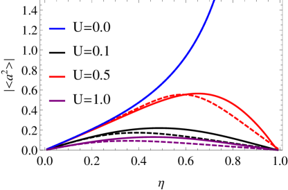
Let us move to the interacting case. We start with the single site case. We anticipate here the main result, which is exportable to the many-body part. There is a competition between the photon-photon interaction, with strength $U$, and the squeezed dissipators $L_{j}$. In the limit: $\omega,U\ll 1$, $\varrho^{*}$ relaxes to a squeezed vacuum state. On the other hand, if $\omega,U\gg 1$, then $\varrho^{*}\sim\prod_{j}{\rm e}^{-\beta^{*}(\omega n_{j}+Un_{j}(n_{j}-1))}$ with $\beta^{*}=1/T^{*}$, an effective temperature (to be defined below). This trade off explains the equilibrium statistics of the model (1) with (2) and (3). Importangly enough the parity symmetry $a_{j}\to-a_{j}$ is not broken, finding always that $\langle a_{j}\rangle=0$. Let us check this picture.

Making $H_{S}=0$, the evolution (1) is given by $\partial_{\tau}\varrho=L\varrho L^{\dagger}-1/2\{LL^{\dagger},\varrho\}$, with $L=a+\eta{\rm e}^{i\phi}a^{\dagger}$ (for the single site). Therefore $\varrho^{*}=|\xi\rangle\langle\xi|$, with $L|\xi\rangle=0$, i.e. the vacuum squeezed state. On the other hand, if $\omega,U\gg 1$, it is convenient to work in the interaction picture (with respect to the $H_{S}$). We have that,

$$VaV^{\dagger}=\sum_{n}{\rm e}^{-i(\omega+2nU)t}|n\rangle\langle n|a$$ (15)

with $V={\rm exp}[i(\omega n+Un(n-1))t]$, i.e., the Hamiltonian rotates each Fock state with a different phase. Using a Rotating Wave-like argument we can expect that the time-dependent terms average to zero. Conserving only the non-rotating terms we have that the quantum master equation (QME) (1) can be approximated by:

$$\dfrac{d\varrho}{d\tau}=\frac{1}{2}(2a\varrho a^{\dagger}-\{a^{\dagger}a,\varrho\})+\frac{\eta^{2}}{2}(2a^{\dagger}\varrho a-\{aa^{\dagger},\varrho\})$$ (16)

Identifying $\eta^{2}=\bar{n}(\omega)/(1+\bar{n}(\omega))$, with $\overline{n}(\omega)$ the Bose distribution $\overline{n}(\omega)={1}/{({\rm e}^{\beta\hbar\omega}-1)}$, the above matches the dissipators for a damped harmonic oscillator in a thermal bath with effective temperature,

$$\beta^{*}\omega=-2\ln\eta\;.$$ (17)

The above argument can be validated and refined. It is not hard to realize that, independently of the value of $U$, we have that:

$$\langle n\rangle_{\varrho^{*}}\equiv\langle a^{\dagger}a\rangle_{\varrho^{*}}=\frac{\eta^{2}}{1-\eta^{2}}$$ (18)

Through the text we use the notation $\langle\cdot\rangle_{\varrho^{*}}\equiv{\rm Tr}(\cdot\,\varrho^{*})$. Notice that by using (17) in (18) we obtain the thermal Bose distribution $\langle n\rangle_{\rho^{*}}=({\rm e}^{\beta^{*}\omega}-1)^{-1}$. Therefore, for the photon number, the state is as it would be thermal state with the temperature predicted by the previous simple argument, Eq. (17).

In obtaining a dynamical equation for other variances, as $\langle a\rangle$ and $\langle a^{2}\rangle$ we find an infinity hierarchy of equations involving higher order averages as $\langle(a^{\dagger})^{n}a^{m}\rangle$. We made use of the HFB or Gaussian approximation, as explained in section III.1. The HFB can be justified a priori as follows. We expect to obtain the Gaussian thermal state $\varrho^{*}\sim{\rm e}^{-\beta^{*}a^{\dagger}a}$ by increasing $U$. On the other hand, whenever $U=0$, the HFB is exact.

Particularizing Eqs. (5) and (7) to the single site case we can write a system of differential equations for $\langle a\rangle$,

$$\dfrac{{\rm d}\langle a\rangle}{{\rm d}t}= \left(-i\omega-\frac{1}{2}(1-\eta^{2})\right)\langle a\rangle$$

$$-2iU\Big{(}2\langle n\rangle\langle a\rangle+\langle a^{2}\rangle\langle a\rangle^{*}-2\langle a\rangle^{*}\langle a\rangle^{2}\Big{)}$$ (19)

and $\langle a^{2}\rangle$

$$\dfrac{{\rm d}\langle a^{2}\rangle}{{\rm d}t}= \left(-i(2\omega+2U+12U\langle n\rangle)-(1-\eta^{2})\right)\langle a^{2}\rangle$$

$$+8iU\langle a\rangle^{*}\langle a\rangle^{3}-\eta{\rm e}^{i\theta}$$ (20)

This, together with (18), can be solved for its steady-state.

Apart from the aforementioned transition to a thermal state, the other key result in this paper is the following. We always find that (See Appendix A for technical details):

$$\langle a\rangle_{\rho^{*}}=0\;.$$ (21)

Therefore, for the single site case and within the HFB, there is not a breaking symmetry state. Recall that the Hamiltonian (2) together with the dissipators (3) have the parity symmetry $a_{i}\to-a_{i}$. Further discussion will be given in IV.3.

The steady-state solution for $\langle a^{2}\rangle$ is given by

$$\langle a^{2}\rangle_{\varrho^{*}}=\frac{-\eta{\rm e}^{i\theta}}{(1-\eta^{2})+i2[U(6\langle n\rangle_{\varrho^{*}}+1)+\omega]}\;.$$ (22)

We see that $\langle a^{2}\rangle_{\varrho^{*}}$ approaches to zero as $U\gg 1$, while $\langle a\rangle_{\rho^{*}}$ and $\langle n\rangle_{\varrho^{*}}$ always equal their thermal averages [Cf. Eqs. (18) and (21)]. Therefore, the Gaussian approximation, in the limit $U\gg 1$, matches the thermal state $\varrho^{*}\sim{\rm e}^{-\beta^{*}a^{\dagger}a}$, as expected.

To validate all this, we perform numerical solutions, as explained in III.3. In figure 1 we show, first, that the HFB captures well the numerical result. Besides, we observe that the squeezing grows with $\eta$ whenever $U=0$ Quijandría et al. (2013). As soon as $U>0$ the state approaches a thermal state with temperature $\beta^{*}\sim-\log\eta$ [Cf. Eq. (17)]. Therefore, $\eta$ favours both squeezing ($U=0$) and high-T thermal states ($U\neq 0$). From this trade-off the maximum for $\langle a^{2}\rangle_{\varrho^{*}}$ in figure 1 is understood.

IV.3 Many body

Figure 2: HFB (left) versus Gutzwiller (right). TOP: $|\langle a^{2}\rangle|$ as a function of $\eta$ and $U/J$. BOTTOM: $\langle n\rangle$ as a function of $\eta$ for some values of $U/J$. For both, HFB and Gutzwiller, we have chosen: $\omega=-2J$ and $\theta=0$. The HFB result considers a linear array with $10$ sites and periodic boundary conditions. For the Gutzwiller solution we have taken a photon cut-off $N_{C}=60$.

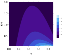
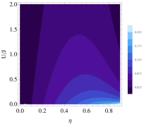
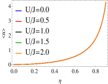
Equipped with the last results, we make a step forward and discuss the many body, i.e. more than one site. In this case, a numerical solution becomes very costly due to the violent growth of the size of the total Hilbert space. This renders the many body problem non tractable numerically. In turn, we have the Gaussian approximation which in the single site case works reasonably well [Cf. Fig. 1 ]. In App. B we also test the HFB for the two site case. Besides, the HFB approximation will be complemented within a Gutzwiller ansatz. Combining both approaches we will capture the main physics.

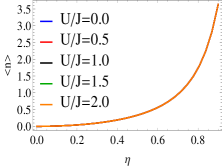
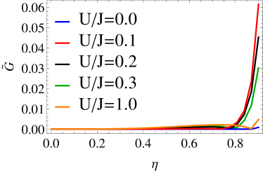
We plot in figure 2 $|\langle a_{j}^{2}\rangle|$ and $\langle a_{j}^{\dagger}a_{j}\rangle$, comparing both approximations. We are assuming translational invariance. For the HFB, systems with $N=10$ sites and periodic boundary conditions have been considered. Thus, these quantities are independent of $j$. As seen in Fig. 2 both Gutzwiller and HFB provide essentially the same results. We compute the non-Gaussianity for the Gutzwiller solution,

$$\tilde{G}:=|\langle a_{j}^{\dagger}a_{j}^{\dagger}a_{j}a_{j}\rangle-\big{(}2\langle a^{\dagger}_{j}a_{j}\rangle^{2}+\langle(a_{j}^{\dagger})^{2}\rangle\langle a_{j}^{2}\rangle-\langle a^{\dagger}_{j}\rangle^{2}\langle a_{j}\rangle^{2}\big{)}|\;,$$ (23)

where the last three terms come from computing the average $\langle a_{j}^{\dagger}a_{j}^{\dagger}a_{j}a_{j}\rangle$ with the Wick formula (4), i.e. assuming a Gaussian distribution. A value of $\tilde{G}$ greater than zero implies that the state is non-Gaussian. In figure 3 it is clearly appreciated that $\tilde{G}$ is always very small. Only in a small region for $\eta\cong 1$ and $U\cong 0.2$, $\tilde{G}$ differentiates from zero.

IV.3.1 Transition to a thermal state

Once the approximations have been tested, let us discuss the main physics occurring. We first discuss the transition to a thermal state, pretty much like for the single site [Cf. section IV.2]. In the limit of large $U$, we again rotate the state as in Eq. (15), having that $Va_{j}V^{\dagger}=\sum_{n}{\rm e}^{-i2n_{j}Ut}|n_{j}\rangle\langle n_{j}|a_{j}$ (in the interaction picture with respect to the self-interaction term). The coupling $a_{j}^{\dagger}a_{j+1}+{\rm h.c.}$ also averages to zero within the RWA argument. Therefore, in the limit $U$ large the effective master equation is as in (16) but summed over all the sites: $\partial_{t}\rho=\frac{1}{2}\sum_{l}(2a_{j}\varrho a_{j}^{\dagger}-\{a_{j}^{\dagger}a_{j},\varrho\})+\frac{\eta^{2}}{2}\sum_{j}(2a_{j}^{\dagger}\varrho a_{j}-\{a_{j}a_{j}^{\dagger},\varrho\})$. The stationary state, then reduces to a thermal state of uncoupled resonators with temperature given by (17). Further confirmation of the above picture within the HFB approximation comes from studying the $X_{ij}$ terms in the thermodynamic limit ($N\to\infty$). Assuming translational invariance it is easy to see that we can obtain a closed set of equations for the diagonal terms of (6)

$$\partial_{t}X_{ii}=-(1-\eta^{2})X_{ii}+\eta^{2}$$ (24)

which generalizes (18) to the multi-site case. In a similar fashion we obtain that,

$$\langle a^{\dagger}_{i}a_{i}\rangle=\frac{1}{{\rm e}^{\beta^{*}\omega}-1}$$ (25)

We stress that the latter is independent of $U$. This explains the non-dependence on $U$ for $a_{j}^{\dagger}a_{j}$ in figure 2.

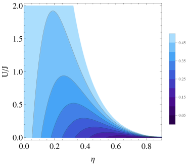
The appearance of this synthetic thermal state can be traced by computing the squeezing. For a thermal state this quadrature must equal $1/2$ (coherent state). In figure 4 we can appreciate this transition. To understand it, we must recall the non-interacting case $U=0$. There, the limit $\eta\to 1$ is a critical point where a couple of modes become a maximally entangled EPR state. In other words, the squeezing is infinite in this point. However as soon as $U\neq 0$ $\varrho^{*}$ approaches to a thermal state, with temperature given by (17), i.e. infinite as $\eta\to 1$. Therefore the squeezing becomes neglible as soon as $U\neq 0$ for such a big $\eta$. For smaller $\eta$ the thermal state has a lower temperature and the squeezing survives for higuer $U$.

Figure 3: Non-Gaussianity $\tilde{G}$ for the Gutzwiller solution (Eq. 23) as a function of $\eta$ for different values of the ratio $U/J$. Plots are shown for: $U/J=0$ (blue), $U/J=0.1$ (red), $U/J=0.2$ (black), $U/J=0.3$ (green) and $U/J=1.0$ (orange). This solution corresponds to $\omega=-2J$, $\theta=0$ and a photon cut-off $N_{C}=60$.

Figure 4: Squeezing (minimum eigenvalue of the covariance matrix) for a many-body array in the HFB approximation. The solution corresponds to a linear array with $10$ sites and periodic boundary conditions. The parameters chosen were $\omega=-2J$ and $\theta=0$. The white area in the plot corresponds to no squeezing - the eigenvalues of the covariance matrix are all greater or equal than $1/2$ (according to the discussion in Sect. IV.1).

IV.3.2 No symmetry breaking

The non dissipative BH model exhibits a $U(1)$ symmetry ($a_{j}\rightarrow a_{j}{\rm e}^{i\phi}$). The latter is broken whenever the expectation value of $a_{j}$ becomes diferent from zero (Mott insulator - superfluid transition Sachdev (2011)). In our case, Eq. (1) does not exhibit this symmetry, but it is symmetric under the parity transformation $a_{j}\to-a_{j}$. We have found that the latter symmetry is never broken, as we always obtain that $\langle a_{j}\rangle=0$.

In the non-interacting case Quijandría et al. (2013), the parity symmetry is not broken and $\langle a_{j}\rangle=0$ always holds. For the single site (section IV.2) we already learnt that this is also the case. We ask ourselves how this picture gets modified as soon as $U\neq 0$, and more sites enter in the game.

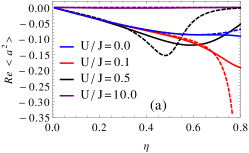
In order to provide a strong argument, we are going to proceed in two directions. First of all, we will follow the HFB approximation by solving the coupled equations (5), (6) and (7). In second place, we will adopt a Gutzwiller ansatz. Here, translational invariance will be also assumed. Even though this condition provides this ansatz of a mean field character, it is important to stress that this approach goes beyond the HFB treatment (as already mentioned, the Gutzwiller ansatz takes fully into account the interaction term). The set of parameters to investigate $(\omega/\Gamma,\theta,\eta,J/\Gamma,U/\Gamma)$ is huge. As we have already verified, the role of the on-site potential is to thermalize the state and therefore destroy the entanglement. Thus, a very favourable set of parameters is the one which maximizes the entanglement for $U/J=0$. This is achieved by setting $\omega=-2J$ and $\theta=0$ (that is, we impose that the zero momentum mode is maximally entangled (squeezed) in the absence of interaction). This seems reasonable due to the following argument. In the Bose-Hubbard model without dissipation, the ground state in the regime $U/J\rightarrow\infty$ is a Mott insulator with a well defined number of excitations per site, thus, $\langle a_{i}\rangle=0$. In the opposite limit $U/J\rightarrow 0$, the ground state is characterized by a Gutzwiller ansatz corresponding to a product state with different particle number per site Rokhsar and Kotliar (1991). Therefore, $\langle a_{i}\rangle\neq 0$. The latter, the superfluid phase, corresponds to the presence of long-range correlations. Long-range ordering (divergent entanglement) in the present setup, is achieved for $U/J=0$ and $\eta=1$. Therefore, we could expect to find a broken symmetry around this configuration. We have always found that $\langle a_{i}\rangle=0$ both in the HFB approximation and the Gutzwiller ansatz. Other parameter regimes were investigated but no symmetry breaking was found. Therefore, as we had anticipated, this model does not exhibit a phase transition.

V Conclusions

We have studied the equilibrium statistics of a Bose Hubbard model with squeezed dissipation. To set in a context, we mention that our model has not an external driving competing with driving, as for example in Le Boité et al. (2013); Grujic et al. (2013); Boité et al. (2014). The driving is, say, incoherent as introduced by the dissipators. In this sense, the physics discussed here has not any time dependence. It is the squeezing, generated via the dissipators, and the Hamiltonian competition which provides the equilibrium phases.

In summary, we have taken as a reference the limit of zero onsite repulsion ($U=0$). This linear model was shown to be critical Quijandría et al. (2013); Eisert and Prosen (2010). In this work we have shown that as soon as $U\neq 0$ correlations shrink to zero. The stationary state approaches a trivial thermal state of uncoupled oscillators. The temperature of this synthetic state is proportional to the squeezing in the dissipators, given by Eq. (17). We emphasize that the dissipators (3) are not $U(1)$-symmetric, but they conserve the parity $a_{j}\to-a_{j}$. Furthermore, it has been shown that $\langle a_{j}\rangle=0$ always. Thus, there is no condensation.

Our findings were based on two approximations, the HFB and the Gutzwiller ansatz. The HFB is a Gaussian approximation [See Sect. III.1]. The Gutzwiller assumes a factorized density matrix as explained in III.2. These approximations can be understood as complementary: the HFB accounts for long distance correlators but it is approximate in the interacting part. On the other hand,the Gutzwiller can not catch long distance correlations but it is exact in the nonlinearities. The physics of the problem treated here provides an agreement between both approximations. The equilibrium state is basically a thermal (Gaussian) state for uncoupled oscillators.

Appendix A Solutions for $\langle a\rangle$

We detail here our steps for checking that $\langle a_{i}\rangle=0$. For the single site case it is possible to argue analytically, the equations (within the HFB approximation) are:

$$\partial_{t}\langle a\rangle =\Big{[}-i\omega-\frac{1}{2}(1-\eta^{2})+2iU|\langle a\rangle|^{2}\Big{]}\langle a\rangle$$ (26)

$$-2iU\Big{(}2\langle n\rangle\langle a\rangle+\langle a^{2}\rangle\langle a\rangle^{*}\Big{)}$$

and,

$$\partial_{t}\langle a^{2}\rangle=\Big{[} -i(2\omega+2U+12U\langle n\rangle)-(1-\eta^{2})\Big{]}\langle a^{2}\rangle$$ (27)

$$+8iU|\langle a\rangle|^{2}\langle a\rangle^{2}-\eta{\rm e}^{i\theta}$$

with $\langle n\rangle=\eta^{2}/(1-\eta^{2})$ as given by Eq. (18). This is a nonlinear set of equations, we did not known how to solve the general case analytically. We are interested in the equilibrium solution. Therefore we are searching for solutions $\partial_{t}\langle a\rangle=0$ and $\partial_{t}\langle a^{2}\rangle=0$.

We realize that $\langle a\rangle=0$ is always a solution of the system, indeed for $U=0$ it is the only solution. We want to check if $\langle a\rangle\neq 0$ is also solution. Assuming continuity, we suppose that for $U\neq 0$ exists $\langle a\rangle=\epsilon$ with $|\epsilon|<<1$. Then, we linearize (26) and (27) discarding the terms with $|\langle a\rangle|^{2}$. Proceeding in this way, (27) becomes a closed equation for $\langle a^{2}\rangle$ with solution given by (22). Formula (22) is introduced in (26) obtaining a linear set for both the real and imaginary parts of $\langle a\rangle$:

$$\left(\begin{array}[]{cc}2U{\rm Im}[\langle a^{2}\rangle]-\frac{1-\eta^{2}}{2}&4U\langle n\rangle-2U{\rm Re}[\langle a^{2}\rangle]\\ -4U\langle n\rangle-2U{\rm Re}[\langle a^{2}\rangle]&-2U{\rm Im}[\langle a^{2}\rangle]-\frac{1-\eta^{2}}{2}\end{array}\right)\;\left(\begin{array}[]{c}{\rm Re}[\langle a\rangle]\\ {\rm Im}[\langle a\rangle]\end{array}\right)=0$$ (28)

In our search for a non-trivial solution, we force the determinant of the above matrix to be zero obtaining the condition:

$$|\langle a^{2}\rangle|^{2}=4\langle n\rangle^{2}+\frac{\eta^{4}}{16U^{2}\langle n\rangle^{2}}$$ (29)

A graphical solution of the above shows that this condition never holds. Indeed we can see that $4\langle n\rangle^{2}+\frac{\eta^{4}}{16U^{2}\langle n\rangle^{2}}>|\langle a^{2}\rangle|^{2}$ always.

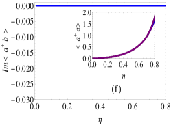
This argument was also tested numerically, searching for solutions to the full nonlinear set of equations (26) and (27). In the range explored $0<U<10$ and $0<\eta<0.99$ the only solution we found was the trivial $\langle a\rangle=0$. If we perform a mean field approximation to the many-body equations, i.e. replacing the hopping term by $J(\langle a_{j}^{\dagger}\rangle a_{j}+{\rm h.c.})$, the problem is reduced to the single site case already discussed. The only difference is that the onsite frequencies get shifted by $\omega\rightarrow\omega+J$. Then, in mean field approximation and within the HFB approximation no broken symmetry is expected. When solving the full set of HFB equations for the multisite case (5-7), we always confirmed that $\langle a_{i}\rangle=0$ for $0<U<1$ and $0<\eta<0.8$.

Appendix B Two site case: A critical analysis of the HFB approximation

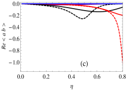
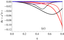
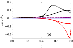
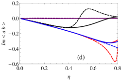
In this appendix we test the HFB for the dimer ($N=2$). We compute the second moments both numerically and within the HFB. We plot the comparison in figure (5). Some comments are relevant. Appealing to our experience with the single site, the population in each site diverges as $\eta\to 1$ in Eq. (18) [See also Fig. 5 f]. Therefore, our numerics fail in this limit. Our accuracy tests do not permit to show results for $\eta>0.8$. In this case we observe that for high nonlinearities ($U\cong 0.5$) the HFB is not accurate at intermediate values of $\eta$ ($0.4<\eta<0.8$). For higher values of $\eta$ we expect things to get better (in fact, the HFB results clearly show this behavior). A similar behavior was found for the single site case. This can be understood on the grounds of the synthetic thermal state approach developed for it. There we observed that, for low values of the nonlinearity and high values of $\eta$, the steady state exhibited the behavior of a thermal state with large temperature $\beta^{*}\sim-\ln\eta$. Increasing the value of $U$ means that $\varrho^{*}$ approaches a thermal state $\sim{\rm e}^{\-\beta\omega\sum a_{j}^{\dagger}a_{j}}$ which is gaussian [Cf. Sect. IV.2].

References

- Breuer and Petruccione (2002) H.-P. Breuer and F. Petruccione, The Theory of Open Quantum Systems (2002).
- Weiss (2008) U. Weiss, Quantum Dissipative Systems, Series in modern condensed matter physics (World Scientific, 2008).
- Rivas and Huelga (2011) Á. Rivas and S. Huelga, Open Quantum Systems: An Introduction, SpringerBriefs in Physics (Springer, 2011).
- Balescu (1975) R. Balescu, Equilibrium and nonequilibrium statistical mechanics (Wiley, 1975).
- Hänggi and Ingold (2005) P. Hänggi and G.-L. Ingold, Chaos (Woodbury, N.Y.) 15, 26105 (2005).
- Pachon et al. (2014) L. A. Pachon, J. F. Triana, D. Zueco, and P. Brumer, , 6 (2014), arXiv:1401.1418 .
- Tomadin et al. (2011) A. Tomadin, S. Diehl, and P. Zoller, Physical Review A 83, 013611 (2011).
- Tomadin et al. (2012) A. Tomadin, S. Diehl, M. D. Lukin, P. Rabl, and P. Zoller, Phys. Rev. A 86, 033821 (2012).
- Horstmann et al. (2013) B. Horstmann, J. I. Cirac, and G. Giedke, Phys. Rev. A 87, 012108 (2013).
- Diehl et al. (2010) S. Diehl, A. Tomadin, A. Micheli, R. Fazio, and P. Zoller, Phys. Rev. Lett. 105, 015702 (2010).
- Eisert and Prosen (2010) J. Eisert and T. Prosen, , 5 (2010), arXiv:1012.5013 .
- Jin et al. (2013) J. Jin, D. Rossini, R. Fazio, M. Leib, and M. Hartmann, Physical Review Letters 110, 163605 (2013).
- Ruiz-Rivas et al. (2014) J. Ruiz-Rivas, E. del Valle, C. Gies, P. Gartner, and M. J. Hartmann, , 9 (2014), arXiv:1401.5776 .
- Jin et al. (2014) J. Jin, D. Rossini, M. Leib, M. J. Hartmann, and R. Fazio, , 11 (2014), arXiv:1404.6063 .
- Le Boité et al. (2013) A. Le Boité, G. Orso, and C. Ciuti, Physical Review Letters 110, 233601 (2013).
- Grujic et al. (2013) T. Grujic, S. R. Clark, D. Jaksch, and D. G. Angelakis, Physical Review A 87, 053846 (2013).
- Boité et al. (2014) A. L. Boité, G. Orso, and C. Ciuti, (2014), arXiv:1408.1330 .
- Dalla Torre et al. (2013) E. G. Dalla Torre, J. Otterbach, E. Demler, V. Vuletic, and M. D. Lukin, Phys. Rev. Lett. 110, 120402 (2013).
- Quijandría et al. (2013) F. Quijandría, D. Porras, J. J. García-Ripoll, and D. Zueco, Phys. Rev. Lett. 111, 073602 (2013).
- Cazalilla et al. (2011) M. Cazalilla, R. Citro, T. Giamarchi, E. Orignac, and M. Rigol, Reviews of Modern Physics 83, 1405 (2011).
- Köhler and Burnett (2002) T. Köhler and K. Burnett, Physical Review A 65, 033601 (2002).
- Rey et al. (2004) A. Rey, B. Hu, E. Calzetta, A. Roura, and C. Clark, Physical Review A 69, 033610 (2004).
- Holland et al. (2001) M. Holland, J. Park, and R. Walser, Physical Review Letters 86, 1915 (2001).
- Proukakis et al. (1998) N. Proukakis, K. Burnett, and H. Stoof, Physical Review A 57, 1230 (1998).
- Griffin (1996) A. Griffin, Physical Review B 53, 9341 (1996).
- Takayoshi et al. (2010) S. Takayoshi, M. Sato, and S. Furukawa, Physical Review A 81, 053606 (2010).
- Tan (2002) S. Tan, A Quantum Optics Toolbox for Matlab 5 (2002).
- Simon et al. (1994) R. Simon, N. Mukunda, and B. Dutta, Phys. Rev. A 49, 1567 (1994).
- Sachdev (2011) S. Sachdev, Quantum phase transitions, second ed. ed. (Cambridge University Press, Cambridge, 2011).
- Rokhsar and Kotliar (1991) D. S. Rokhsar and B. G. Kotliar, Phys. Rev. B 44, 10328 (1991).