Completing the picture for the smallest eigenvalue of real Wishart matrices

Abstract

Rectangular real $N\times(N+\nu)$ matrices $W$ with a Gaussian distribution appear very frequently in data analysis, condensed matter physics and quantum field theory. A central question concerns the correlations encoded in the spectral statistics of $WW^{T}$. The extreme eigenvalues of $WW^{T}$ are of particular interest. We explicitly compute the distribution and the gap probability of the smallest non-zero eigenvalue in this ensemble, both for arbitrary fixed $N$ and $\nu$, and in the universal large $N$ limit with $\nu$ fixed. We uncover an integrable Pfaffian structure valid for all even values of $\nu\geq 0$. This extends previous results for odd $\nu$ at infinite $N$ and recursive results for finite $N$ and for all $\nu$. Our mathematical results include the computation of expectation values of half integer powers of characteristic polynomials.

Introduction. To study generic statistical features of spectra, various kinds of random matrices are used. Following Wigner and Dyson Dyson1962 , Hamiltonians of dynamical systems are modelled by real–symmetric, Hermitian or self-dual matrices in quantum chaos, many-body and mesoscopic physics. Due to universality, cf.  Guhr1998189 ; handbook and references therein, Gaussian probability densities suffice, leading to the Gaussian Orthogonal, Unitary and Symplectic Ensemble (GOE, GUE, GSE) Mehta . This concept was extended to Dirac spectra ShuryakVerbaarschot by imposing chiral symmetry as an additional constraint, resulting in the chiral ensembles chGOE, chGUE, chGSE Verbaarschot1994 . Wishart Wishart put forward random matrices to model spectra of correlation matrices in a quite different context. There are many applications in time series analysis Muirhead ; Anderson ; Chatfield (including chaotic dynamics VP ), in a wide range of fields in physics Guhr1998189 ; handbook , biology Seba , wireless communication TV and finance Plerou . In the most relevant case, $N\times(N+\nu)$ real matrices $W$ model time series such that $WW^{T}$ is the random correlation matrix. If it fluctuates around a given average correlation matrix $C$, the distribution reads

$${\mathbb{P}}_{N,\nu}(W|C)\sim\exp\left[-\mbox{Tr}WW^{T}C^{-1}/2\right]\ .$$ (1)

For $C=\leavevmode\hbox{\small 1\kern-3.8pt\normalsize 1}_{N}$, this happens to coincide with the chGOE, where $W$ and $W^{T}$ model the non–zero blocks of the Dirac operator. Closing the circle, one can also extend Wishart’s model by using non-Gaussian weights. Here and in the sequel, we focus on Eq. (1) with $C=\leavevmode\hbox{\small 1\kern-3.8pt\normalsize 1}_{N}$. Since $WW^{T}$ has positive eigenvalues, the spectrum is bounded from below. Naturally, the distribution of the smallest (non–zero) eigenvalue is of particular importance.

Much interest in the chGOE was sparked by the observation Jac that in the limit $N\to\infty$ its spectral correlators describe the Dirac spectrum in quantum field theories with real Fermions and broken chiral symmetry, see Verbaarschot:2000 for a review. Based on earlier works for finite $N$ Mahoux ; NW , the spectral density Jac and all higher density correlation functions NF95 were computed in terms of a Pfaffian determinant of a matrix kernel for all $\nu$. These quantities were shown later to be universal Klein for non-Gaussian potentials, and most recently for fixed trace ensembles in the context of quantum entanglement, see AV and references therein. Further applications of the chGOE can be found in the recent review carlo on Majorana Fermions and topological superconductors.

In an influential paper Edelman88 the condition number of a Wishart random matrix $WW^{T}$ was investigated, that is the root of the ratio of the largest over the smallest non-zero eigenvalue of $WW^{T}$. This quantity is important for a generic matrix as it quantifies the difficulty of computing its inverse. In Edelman the distribution of the smallest eigenvalue was calculated recursively in $N$ for arbitrary rectangular chGOE matrices. Closed expressions were given for quadratic matrices $\nu=0$ Edelman88 (cf. Peter93 ) and for $\nu=1,2,3$ Edelman . Later Pfaffian expressions were found in NF98 for arbitrary odd $\nu$ valid for fixed and asymptotically large $N$. A more general consideration, including correlations with $C\neq\leavevmode\hbox{\small 1\kern-3.8pt\normalsize 1}_{N}$, of the smallest eigenvalue for $\nu$ odd was given in WG . The limiting distributions of the $k$-th smallest eigenvalue were computed in DN01 , again for $\nu$ odd. These quantities are an efficient tool to test algorithms with exact chiral symmetry in lattice gauge theories Edwards , distinguishing clearly between different topologies labelled by $\nu$. In BLP the distributions for higher even $\nu>0$ were obtained from numerical chGOE simulations. Most recently efficient numerical algorithms have been applied, see e.g. SMN , in order to compute smallest eigenvalue distributions for arbitrary $\nu$ using known analytic Fredholm determinant expressions Peter06 .

It is our goal to complete the picture for the smallest chGOE eigenvalue distribution and its integral by finding explicit Pfaffian expressions for finite and infinite $N$ valid for all even $\nu$. Together with previous results this completes the integrability of this classical ensemble. A presentation with further results and more mathematical details will be given elsewhere AKWW .

Smallest eigenvalue and gap probability. First we define the quantities of interest and state the problem. In the analytic calculations below we set $C=\leavevmode\hbox{\small 1\kern-3.8pt\normalsize 1}_{N}$ in Eq. (1), and later we compare our universal large $N$ results to numerical simulations with $C\neq\leavevmode\hbox{\small 1\kern-3.8pt\normalsize 1}_{N}$. Because we are only interested in correlations of the positive eigenvalues of $WW^{T}=OXO^{T}$ contained in $X=\mbox{diag}(x_{1},\ldots,x_{N})$, we drop all normalisation constants depending on the orthogonal matrix $O$. Integrating the distribution (1) over all independent matrix elements with respect to flat Lebesgue measure we obtain the partition function expressed in terms of the eigenvalues as

$${\cal Z}_{N,\gamma}=\prod_{i=1}^{N}\int_{0}^{\infty}dx_{i}w_{\gamma}(x_{i})\ |\Delta_{N}(X)|\ ,$$ (2)

up to a known constant. Here we introduce the weight function $w_{\gamma}(x)$ and Vandermonde determinant $\Delta_{N}(X)$ stemming from the Jacobian of the diagonalisation,

$$w_{\gamma}(x) \equiv x^{\gamma}\exp[-x/2]\ ,\ \gamma\equiv{(\nu-1)/2}\ ,$$ (3)

$$\Delta_{N}(X) \equiv \prod_{1\leq i<j\leq N}(x_{j}-x_{i})=\det_{1\leq i,j\leq N}\left[x_{i}^{j-1}\right].$$ (4)

We note that $\gamma$ alternates between integer and half-integer values. The expectation value of an observable $f$ only depending on $X$ is defined as

$$\langle f(X)\,\rangle_{N,\gamma}\equiv\frac{\prod_{i=1}^{N}\int_{0}^{\infty}dx_{i}w_{\gamma}(x_{i})\ f(X)|\Delta_{N}(X)|}{{\cal Z}_{N,\gamma}}.$$ (5)

Thus the gap probability that no eigenvalue occupies the interval $[0,t]$ is given by

$${E}_{N,\gamma}(t) \equiv \frac{1}{{\cal Z}_{N,\gamma}}\prod_{i=1}^{N}\int_{t}^{\infty}dx_{i}w_{\gamma}(x_{i})\ |\Delta_{N}(X)|$$ (6)

$$= \mbox{e}^{-Nt/2}\frac{{\cal Z}_{N,0}}{{\cal Z}_{N,\gamma}}\left\langle{\det}^{\gamma}[X+t\leavevmode\hbox{\small 1\kern-3.8pt\normalsize 1}_{N}]\right\rangle_{N,0}\ .$$

It is expressed as an expectation value of a characteristic polynomial to the power $\gamma$ with respect to the weight function (3) without the pre-exponential factor, $w_{0}(x)$. This crucial identity follows from the translation invariance of the Vandermonde determinant (4).

The normalised distribution of the smallest non-zero eigenvalue, ${P}_{N,\gamma}(t)$, is obtained by differentiating Eq. (6)

$${P}_{N,\gamma}(t) \equiv -\frac{\partial{E}_{N,\gamma}(t)}{\partial t}$$

$$= t^{\gamma}\mbox{e}^{-{Nt}/{2}}\frac{N{\cal Z}_{N-1,1}}{{\cal Z}_{N,\gamma}}\left\langle{\det}^{\gamma}[X+t\leavevmode\hbox{\small 1\kern-3.8pt\normalsize 1}_{N-1}]\right\rangle_{N-1,1},$$

where the second line follows along the same steps as in Eq. (6). This relation is well known NF98 ; DN01 , with the difficulty to compute the average (also called massive partition function) for $\gamma$ half-integer, which is our main task.

To compute Eqs. (6) and ( Completing the picture for the smallest eigenvalue of real Wishart matrices) we need to know the normalising partition functions, which are given for arbitrary real $\nu>-1$ in terms of the Selberg integral, see also NN ; AK , and the expectation values. For integer $\gamma=k$ corresponding to odd $\nu=2k+1$ closed expressions of ( Completing the picture for the smallest eigenvalue of real Wishart matrices) exist NF98 , given in terms of Laguerre polynomials skew-orthogonal with respect to the weight (3). Therefore we concentrate on the case $\nu=2k$ even.

Pfaffian structure and finite $N$ results. To show that the gap probability (6) has a Pfaffian structure when $\gamma$ is half-integer let us define the following parameter dependent weight function

$$w(x;t)\equiv\exp[-\eta x/2]/\sqrt{x+t}\ .$$ (8)

It absorbs the half-integer part in the expectation value (6) when $\nu=2k$ is even. We set $\eta=1$ unless otherwise stated. The monic polynomials $R_{k}(x;t)=x^{k}+\ldots$ are defined to be skew-orthogonal with respect to the following skew-symmetric scalar product

$$\left<f,g\right>_{t}\equiv\int\limits^{\infty}_{0}\!\!dy\int\limits_{0}^{y}\!\!dx\,w(x;t)w(y;t)[f(x)g(y)-f(y)g(x)]$$ (9)

by satisfying for all $i,j=0,1,\ldots$ footnote1 the conditions

$$\left<R_{2j},R_{2i}\right>_{t} = 0=\left<R_{2j+1},R_{2i+1}\right>_{t}\$$

$$\left<R_{2j+1},R_{2i}\right>_{t} = r_{j}(t)\ \delta_{ij}\ .$$ (10)

Their normalisations $r_{j}(t)$ depend on $t$. The partition function ${\cal Z}_{N}(t)$ of this new weight (8) is defined by

$${\cal Z}_{N}(t)\equiv\prod_{i=1}^{N}\int_{0}^{\infty}dx_{i}w(x_{i};t)|\Delta_{N}(X)|=N!\prod_{i=0}^{\frac{N}{2}-1}r_{i}(t).$$ (11)

The last step holds for $N$ even Mehta . Likewise we define expectation values $\langle f(X)\rangle_{N}^{t}$, following Eq. (5). Thus for even $\nu=2k$, $k\in\mathbb{N}$, Eq. (6) reduces to

$${E}_{N,k-\frac{1}{2}}(t)=\mbox{e}^{-{Nt}/{2}}\frac{{\cal Z}_{N}(t)}{{\cal Z}_{N,k-\frac{1}{2}}}\left\langle{\det}^{k}[X+t\leavevmode\hbox{\small 1\kern-3.8pt\normalsize 1}_{N}]\right\rangle_{N}^{t},$$ (12)

given in terms of an integer power of a characteristic polynomial. While the skew-orthogonal polynomials with respect to the weight (3) are know in terms of Laguerre polynomials NF98 , the difficulty here is to determine the $t$-dependent polynomials and normalisation constants for the non-standard weight (8). They can be computed following the observation Eynard

$$R_{2j}(y,t) = \left\langle{\det}[X-y\leavevmode\hbox{\small 1\kern-3.8pt\normalsize 1}_{2j}]\right\rangle_{2j}^{t}\ ,$$ (13)

$$R_{2j+1}(y,t) = \left\langle(y+c+\mbox{Tr}X){\det}[X-y\leavevmode\hbox{\small 1\kern-3.8pt\normalsize 1}_{2j}]\right\rangle_{2j}^{t}$$ (14)

$$= (y+c)R_{2j}(y,t)-2\left.\frac{\partial}{\partial\eta}R_{2j}(y,t)\right|_{\eta=1}\!\!\!\!\!.\ \ \ \ \$$

The odd polynomials are obtained by differentiation of the weight (8), generating $\mbox{Tr}X$ in the average. Note that the $R_{2j+1}(y,t)$ are not unique Eynard , we set $c=0$ in the following. The even polynomials (13) can be calculated by mapping them back to a proper matrix integral over an auxiliary $2j\times(2j+1)$ matrix $\overline{W}$ (corresponding to $\gamma=0$),

$$R_{2j}(y,t)=C_{2j}(t)\int d\overline{W}\frac{\det[\overline{W}\overline{W}^{T}-y\leavevmode\hbox{\small 1\kern-3.8pt\normalsize 1}_{2j}]}{\det^{\frac{1}{2}}[\overline{W}\overline{W}^{T}+t\leavevmode\hbox{\small 1\kern-3.8pt\normalsize 1}_{2j}]}\mbox{e}^{-\frac{\eta}{2}\mbox{Tr}\overline{W}\overline{W}^{T}},$$ (15)

cf. WG . The known normalisation constant $C_{2j}(t)$ follows from the fact that the polynomial is monic. Without giving details Eq. (15) can be computed exactly, representing the determinants by Gaussian integrals over commuting and anti-commuting variables and by using standard bosonisation techniques SW . We arrive at

$$R^{a}_{2j}(y,t)=\frac{(2j)!\left(\text{U}_{j}(t){L}^{(a+1)}_{2j-a}(y)-\text{U}^{\prime}_{j}(t){L}^{(a)}_{2j-a}(y)\right)}{(2j-a)!\text{U}\left(\frac{2j+1}{2},\frac{3}{2},\frac{t}{2}\right)}$$ (16)

for the $a$-th derivatives of the polynomials, $\frac{\partial^{a}}{\partial y^{a}}R_{j}(y,t)\equiv R^{a}_{j}(y,t)$, $a=0,1,\ldots$ needed later. Here $\text{U}_{j}(t)\equiv\text{U}\left(\frac{2j+1}{\textbullet 2},\frac{1}{2},\frac{t}{2}\right)$ denotes the Tricomi confluent hypergeometric function, satisfying $\text{U}^{\prime}(a,b,t)=-a\text{U}(a+1,b+1,t)$ NIST . The derivative in Eq. (16) acts only on the generalised Laguerre polynomials used in monic normalisation ${L}^{(a)}_{j}(y)=y^{j}+\ldots$ They satisfy $\frac{\partial^{a}}{\partial y^{a}}{L}^{(b)}_{n}(y)=\frac{n!}{(n-a)!}{L}^{(b+a)}_{n-a}(y)$, where we set ${L}^{(b)}_{n}(y)\equiv 0$ for $n<0$. For the odd polynomials we obtain

$$R^{a}_{2j+1}(y,t)=\left(4j^{2}+4j+y\right)R^{a}_{2j}(y,t)+aR^{a-1}_{2j}(y,t)$$

$$+\frac{(2j)!/(2j-a)!}{\text{U}\left(\frac{2N+1}{2},\frac{3}{2},\frac{t}{2}\right)}\left\{t\text{U}^{\prime\prime}_{j}(t){L}^{(a)}_{2j-a}(y)+2\text{U}^{\prime}_{j}(t)\right.$$

$$\times\left[a{L}^{(a)}_{2j-a}(y)+(2j-a)y{L}^{(a+1)}_{2j-a-1}(y)+\tfrac{t}{2}{L}^{(a+1)}_{2j-a}(y)\right]$$

$$\left.-2\text{U}_{j}(t)\left[a{L}^{(a+1)}_{2j-a}(y)+(2j-a)y{L}^{(a+2)}_{2j-a-1}(y)\right]\right\},$$ (17)

and the normalisation constants in Eq. (10) read

$$r_{j}(t)=2(2j)!(2j+1)!\frac{\text{U}\left(\frac{2j+3}{2},\frac{3}{2},\frac{t}{2}\right)}{\text{U}\left(\frac{2j+1}{2},\frac{3}{2},\frac{t}{2}\right)}~{}.$$ (18)

Following NF98 with their Laguerre weight $w_{0}(x)$ in Eq. (3) replaced by our weight (8), we express the gap probability (12) as a Pfaffian determinant with our kernel consisting of the skew-orthogonal polynomials (16) and (17). In a more general setting averages of characteristic polynomials such as Eq. (12) were considered in Refs. BS ; KG for arbitrary but unspecified weights. For finite even $N$ and $\nu=2k$ with $k=2m$ even we obtain

$${E}_{N,k-\frac{1}{2}}(t)=\mathcal{C}_{N,\nu}\sqrt{t}\ \mbox{e}^{-Nt/2}\text{U}\left(\frac{N+2m+1}{2},\frac{3}{2},\frac{t}{2}\right)$$

$$\times\mbox{Pf}\left[\sum_{j=0}^{\frac{N}{2}+m-1}\frac{R^{a}_{2j+1}\left(-t,t\right)R^{b}_{2j}\left(-t,t\right)-(a\leftrightarrow b)}{r_{j}(t)}\right]_{a,b=0}^{k-1}$$ (19)

For $k\!=\!2m-1$ odd the last row (and column) inside the Pfaffian is replaced by $(-)R^{b(a)}_{N+k-2}(-t,t)/r_{N/2+m-1}(t)$, respectively (for $N$ odd cf. AKWW ). The known $t$-independent constant $\mathcal{C}_{N,\nu}$ is suppressed for simplicity, it ensures ${E}_{N,k-\frac{1}{2}}(t=0)=1$.

Figure 1: The gap probability ${E}_{N,(\nu-1)/2}(t)$ (straight lines) for finite $N=10$ and $\nu=0,2,4,6,8$ (from left to right) vs. numerical simulations (symbols) of $40000$ realisations of Wishart matrices, with $C=\leavevmode\hbox{\small 1\kern-3.8pt\normalsize 1}_{N}$.

Eq. (19) is our first main result. A similar answer can be obtained for ${P}_{N,\gamma}(t)$ for even $\nu$, given in terms of skew-orthogonal polynomials with respect to the weight $x\,w(x;t)$. This provides an explicit integrable Pfaffian structure for both ${E}_{N,\gamma}(t)$ and ${P}_{N,\gamma}(t)$. It extends the odd $\nu$ result for ${P}_{N,\gamma}(t)$ in NF98 which is given by a Pfaffian determinant as well, but with a different kernel.

For illustration we give two examples. For $\nu=0$ the Pfaffian in Eq. (19) is absent,

$${E}_{N,-\frac{1}{2}}(t)=\frac{(N-1)!\sqrt{t}\ \mbox{e}^{-Nt/2}}{2^{N-1/2}\Gamma(N/2)}\text{U}\left(\frac{N+1}{2},\frac{3}{2},\frac{t}{2}\right),$$ (20)

whereas for $\nu=2$ the kernel is absent, and only the polynomial (16) with $a=0$ contributes,

$${E}_{N,+\frac{1}{2}}(t) = \frac{\Gamma\left(\frac{N+1}{2}\right)\sqrt{t}\ \mbox{e}^{-Nt/2}}{(-1)^{N}\sqrt{2\pi}N!}$$

$$\times\left[\text{U}_{N}(t){L}_{N}^{(1)}(-t)-\text{U}^{\prime}_{N}(t){L}_{N}^{(0)}(-t)\right].$$

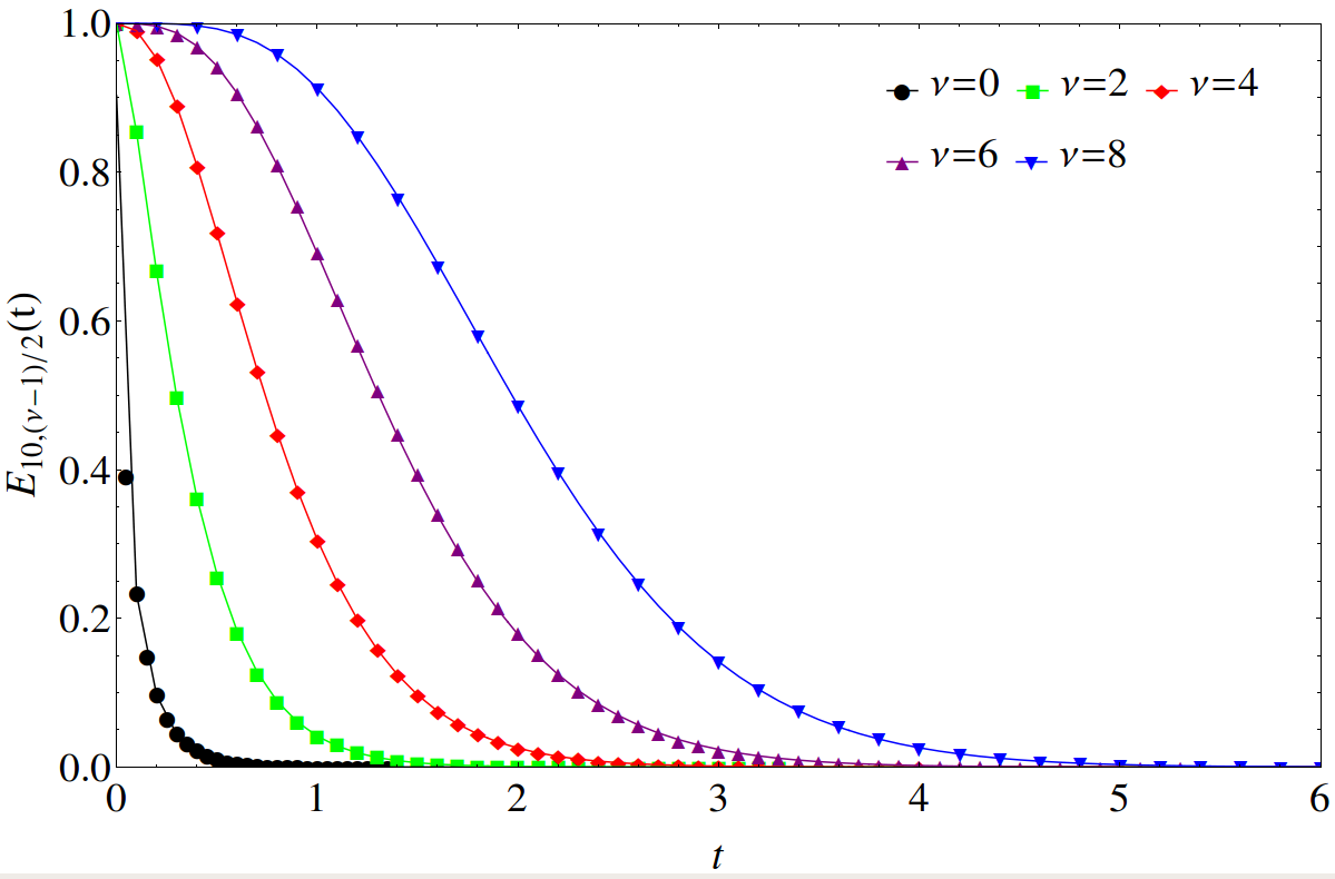
Eqs. (20) and ( Completing the picture for the smallest eigenvalue of real Wishart matrices) are compared to numerical simulations in Fig. 1. They can be matched with the finite $N$ results of Edelman for $\nu=0,2$, after differentiating them and using identities for the Tricomi function NIST .

Figure 2: The microscopic density $\rho(u)$ (30) (dashed lines) vs. the corresponding smallest eigenvalue distribution ${\cal P}_{(\nu-1)/2}(u)$ (straight lines) for $\nu=2,4,6$ (from left to right). The smallest eigenvalue nicely follows the density for all $\nu$.

Microscopic large $N$ limit. We turn to the large $N$ limit keeping $\nu$ fixed, referred to as hard edge limit. It is particularly important as the limiting density correlation functions are universal for non-Gaussian weight functions for any integer $\nu$ Klein . Because the gap probability can be expressed in terms of the limiting universal kernel Peter06 (see Eq. (36) for the corresponding density), its universality carries over to the distribution of the smallest eigenvalue. Moreover, in WG it was shown for both $\nu$ even and odd, without explicitly calculating the distributions, that the presence of a nontrivial correlation matrix in Eq. (1) does not change the limiting smallest eigenvalue distribution when the spectrum of $C$ has a finite distance to the origin.

The limiting gap probability and smallest eigenvalue distribution are defined as

$${\cal E}_{\gamma}(u)\equiv\lim_{N\to\infty}E_{N,\gamma}\left(t=\frac{u}{4N}\right),\ \frac{\partial}{\partial u}{\cal E}_{\gamma}(u)=-{\cal P}_{\gamma}(u)~{}.$$ (22)

In view of Eq. (19) we need the following asymptotic limit of the hypergeometric function,

$$\text{U}\left(aN+c,b,\frac{u}{8N}\right)\approx\frac{2\left(N^{2}{8a}/{u}\right)^{(b-1)/2}}{\Gamma\left(aN+c\right)}\text{K}_{b-1}\left(\sqrt{\frac{au}{4}}\right).$$ (23)

For half integer index the modified Bessel function of second kind simplifies, e.g. for $b=1/2,3/2,5/2$

$$K_{\pm\frac{1}{2}}(z)=\sqrt{\frac{\pi}{2z}}\ \mbox{e}^{-z},\ K_{\frac{3}{2}}(z)=(1-z^{-1})K_{\frac{1}{2}}(z)\ .$$ (24)

Inside the Pfaffian (19) the sum is replaced by an integral, $\sum_{j}\to\frac{N}{2}\int_{0}^{1}dx$, with $j=Nx/2$. The limiting skew-orthogonal polynomials follow from Eq. (23) together with the standard Laguerre asymptotic in terms of modified Bessel functions of the first kind, see e.g. NIST . This leads to the following limiting kernel inside the Pfaffian (19), independently of $N$ being even or odd,

$$\kappa_{ab}(u)\equiv\int_{0}^{u}\frac{dz}{u}z^{(a+b)/2}\left[2(b-a)\text{I}_{a}(\sqrt{z})\text{I}_{b}(\sqrt{z})\right.$$ (25)

$$\left.+(2b+1)\text{I}_{a+1}(\sqrt{z})\text{I}_{b}(\sqrt{z})-(2a+1)\text{I}_{b+1}(\sqrt{z})\text{I}_{a}(\sqrt{z})\right].$$

The final answer for the limiting gap probability reads

$${\cal E}_{k-1/2}(u)=C_{e}\ \mbox{e}^{-\sqrt{u}/2-u/8}\mbox{Pf}\left[\kappa_{ab}(u)\right]_{a,b=0}^{k-1}$$ (26)

for $\nu=2k$ with $k=2m$ even and

$${\cal E}_{k-1/2}(u)=C_{o}\ \mbox{e}^{-\sqrt{u}/2-u/8}$$ (27)

$$\times\mbox{Pf}\left[\begin{array}[]{r}\kappa_{ab}(u)\ \ \ -u^{a/2}\left[\text{I}_{a+1}\left(\sqrt{u}\right)+\text{I}_{a}\left(\sqrt{u}\right)\right]\\ u^{b/2}\left[\text{I}_{b+1}\left(\sqrt{u}\right)+\text{I}_{b}\left(\sqrt{u}\right)\right]\ \ \ \ \ \ \ \ \ \ \ \ \ \ 0\\ \end{array}\right]_{a,b=0}^{k-1}$$ (30)

for $k=2m-1$ odd. We suppress the known $u$-independent normalisation constants $C_{e/o}$.

Figure 3: The microscopic smallest eigenvalue distribution ${\cal P}_{(\nu-1)/2}(u)$ (straight lines) for $\nu=0,2,4$ (from left to right) vs. numerical simulations (symbols) of $10000$ realisations of matrices with $N=200$ and correlation matrix $C\neq\leavevmode\hbox{\small 1\kern-3.8pt\normalsize 1}_{N}$ as indicated in the inset.

The corresponding limiting result for the smallest eigenvalue distribution is

$${\cal P}_{k-1/2}(u)=\widehat{C}_{e}u^{k}(1+2/\sqrt{u})\,\mbox{e}^{-\sqrt{u}/2-u/8}\mbox{Pf}\left[\widehat{\kappa}_{ab}(u)\right]_{a,b=0}^{k-1}$$ (31)

for $\nu=2k$ with $k=2m$ even, and

$${\cal P}_{k-1/2}(u)=\widehat{C}_{o}u^{k}(1+2/\sqrt{u})\,\mbox{e}^{-\sqrt{u}/2-u/8}$$ (32)

$$\times\mbox{Pf}\left[\begin{array}[]{r}\widehat{\kappa}_{ab}(u)\ \ \ -\frac{\text{I}_{a+2}\left(\sqrt{u}\right)+\frac{\sqrt{u}}{2+\sqrt{u}}\text{I}_{a+3}\left(\sqrt{u}\right)}{u^{(a+2)/2}}\\ \frac{\text{I}_{b+2}\left(\sqrt{u}\right)+\frac{\sqrt{u}}{2+\sqrt{u}}\text{I}_{b+3}\left(\sqrt{u}\right)}{u^{(b+2)/2}}\ \ \ \ \ \ \ \ \ \ \ \ \ \ 0\\ \end{array}\right]_{a,b=0}^{k-1}$$ (35)

for $k=2m-1$ odd, suppressing again the $u$-independent normalisation constants $\widehat{C}_{e/o}$. Here $\widehat{\kappa}_{ab}(u)$ is the limiting kernel for the skew-orthogonal polynomials with respect to $x\,w(x;t)$ which is of a similar structure as Eq. (25). For $\nu=0,2$ the results (31) and (32) were known from Peter93 , AV , respectively.

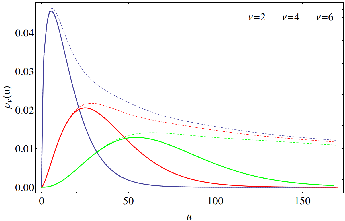
Eqs. (26) - (32) constitute our second main result and are universal. In Fig. 2 they are compared to the universal microscopic density Jac ; FNH valid for all $\nu$-values

$$\rho_{\nu}(u) = \frac{1}{4}\left(J_{\nu}(\sqrt{u})^{2}-J_{\nu-1}(\sqrt{u})J_{\nu+1}(\sqrt{u})\right)$$ (36)

$$+\frac{1}{4\sqrt{u}}J_{\nu}(\sqrt{u})\left(1-\int_{0}^{\sqrt{u}}dsJ_{\nu}(s)\right)~{}.$$

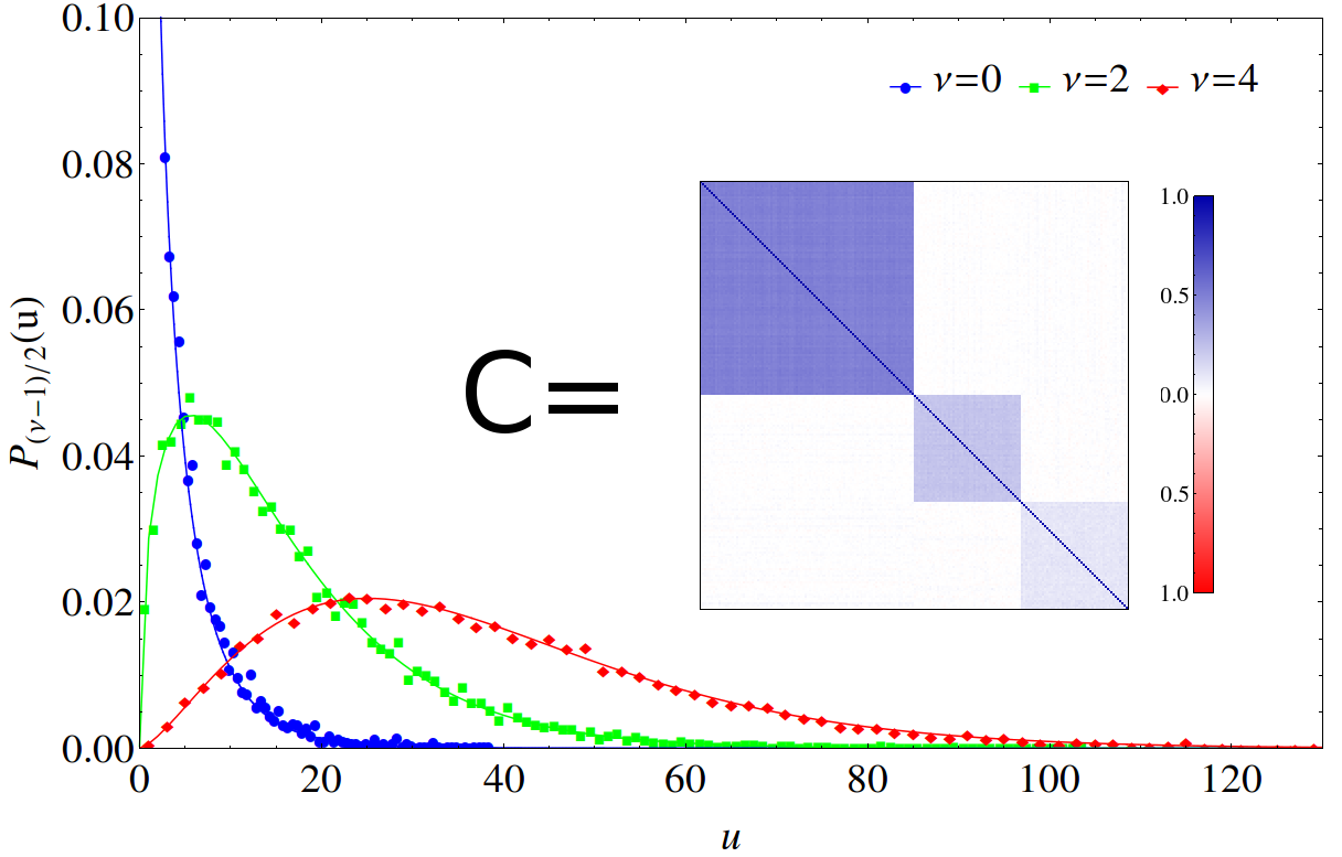
We further illustrate the universality of our results by comparing to numerical simulations with a nontrivial correlation matrix $C$ for large $N$, see Fig. 3.

Conclusions and outlook. We have computed closed expressions for the distribution of the smallest non-zero eigenvalue and its integral, the gap probability, for rectangular $N\times(N+\nu)$ real Wishart matrices with $\nu$ even, both for finite $N$ and in the universal microscopic large $N$ limit. They only depend on a single kernel instead of three different ones for the density correlation functions and are thus much simpler than these known results. We confirm our findings by numerical simulations even including a nontrivial correlation matrix $C$. This completes the calculation of all eigenvalue correlation functions in this classical ensemble of random matrices and shows its integrable structure. Furthermore, our finite $N$ results allow to analyse deviations from the universal large $N$ limit, as was very recently proposed in EGP for the chGUE.

Acknowledgements. We thank the Sonderforschungsbereich TR12 (G.A., T.G. and T.W.) and the Alexander von Humboldt-Foundation (M.K.) for support.

References

- (1) F.J. Dyson, J. Math. Phys. 6 (1962) 1199.
- (2) The Oxford Handbook of Random Matrix Theory, G. Akemann, J. Baik, P. Di Francesco (Eds.), Oxford Univ. Press, Oxford 2011.
- (3) T. Guhr, A. Mueller-Groeling, H.A. Weidenmüller, Phys. Rep. 299 (1998) 189.
- (4) M.L. Mehta, Random Matrices, Academic Press, 3rd ed., London 2004.
- (5) E.V. Shuryak and J.J.M. Verbaarschot, Nucl. Phys. A 560 (1993) 306; J.J.M. Verbaarschot, Phys. Rev. Lett. 72 (1994) 2531.
- (6) J. Verbaarschot , Phys. Rev. Lett. 72 (1994) 2531.
- (7) J. Wishart, Biometrika 20A (1928) 32.
- (8) R.J. Muirhead, Aspects of Multivariate Statistical Theory, Wiley Intersience, Hoboken, NJ 2005.
- (9) T.W. Anderson An Introduction to Multivariate Statistical Analysis, Wiley, New York 2003.
- (10) C. Chatfield, The Analysis of Time Series: An Introduction, Chapman and Hall/CRC, 6th ed., Boca Raton 2003.
- (11) Vinayak, A. Pandey, Phys. Rev. E81 (2010) 036202.
- (12) P. Šeba, Phys. Rev. Lett., 91 (2003) 198104.
- (13) A.M. Tulino, S. Verdu, J. Comm. Infor. Th. 1 (2004) 1.
- (14) V. Plerou et al., Phys. Rev. E65 (2002) 066126.
- (15) J. Verbaarschot, Nucl. Phys. B426 (1994) 559.
- (16) J.J.M. Verbaarschot, T. Wettig, Ann. Rev. Nucl. Part. Sci. 50 (2000) 343.
- (17) G. Mahoux, M. Mehta, J. Phys I France 1 (1991) 1093.
- (18) T. Nagao, M. Wadati, J. Phys. Soc. Japan 60 (1991) 2998.
- (19) T. Nagao, P.J. Forrester, Nucl. Phys. B435 [FS] (1995) 401.
- (20) B. Klein, J.J.M. Verbaarschot, Nucl. Phys. B588 (2000) 483.
- (21) G. Akemann, P. Vivo, J. Stat. Mech. 1105 (2011) P05020.
- (22) C.W.J. Beenakker, arXiv:1407.2131.
- (23) A. Edelman, SIAM J. Matrix Anal. Appl. 9 (1988) 543.
- (24) A. Edelman, Lin. Alg. Appl. 159 (1991) 55.
- (25) P.J. Forrester, Nucl. Phys. B402 (1993) 709.
- (26) T. Nagao, P.J. Forrester, Nucl. Phys. B509 [FS] (1998) 561.
- (27) T. Wirtz, T. Guhr, Phys. Rev. Lett. 111 (2013) 094101; J. Phys. A: Math. Theor. 47 (2014) 075004.
- (28) P.H. Damgaard, S.M. Nishigaki, Phys. Rev. D63 (2001) 045012.
- (29) R.G. Edwards, U.M. Heller, J. Kiskis, R. Narayanan, Phys. Rev. Lett. 82 (1999) 4188.
- (30) P.V. Buividovich, E.V. Luschevskaya, M.I. Polikarpov, Phys. Rev. D78 (2008) 074505.
- (31) S.M. Nishigaki, Phys. Rev. D86 (2012) 114505.
- (32) P.J. Forrester, Forum Math. 18 (2006) 711.
- (33) T. Wirtz, G. Akemann, T. Guhr, M. Kieburg, R. Wegner, unpublished (2014).
- (34) T. Nagao, S.M. Nishigaki, Phys. Rev. D62 (2000) 065006.
- (35) G. Akemann, E. Kanzieper, Phys. Rev. Lett. 85 (2000) 1174.
- (36) For odd an additional condition has to be imposed, , cf. Mehta .
- (37) B. Eynard, J. Phys. A. 34 (2001) 7591.
- (38) L. Schäfer, F.Wegner, Z. Phys. B 38 (1980) 113.
- (39) NIST Handbook of Mathematical Functions, F.W.J. Olver, D.W. Lozier, R.F. Boisvert, C.W. Clark (Eds.), Cambridge Univ. Press, Cambridge 2010.
- (40) A. Borodin, E. Strahov, Comm. Pure Appl. Math. 59 (2006) 161.
- (41) M. Kieburg, T. Guhr, J. Phys. A43 (2010) 135204.
- (42) P.J. Forrester, T. Nagao, G. Honner, Nucl. Phys. B553 (1999) 601.
- (43) A. Edelman, A. Guionnet, S. Péché, arXiv:1405.7590.