Analysis of Spin Financial Market by GARCH Model

Abstract

A spin model is used for simulations of financial markets. To determine return volatility in the spin financial market we use the GARCH model often used for volatility estimation in empirical finance. We apply the Bayesian inference performed by the Markov Chain Monte Carlo method to the parameter estimation of the GARCH model. It is found that volatility determined by the GARCH model exhibits ”volatility clustering” also observed in the real financial markets. Using volatility determined by the GARCH model we examine the mixture-of-distribution hypothesis (MDH) suggested for the asset return dynamics. We find that the returns standardized by volatility are approximately standard normal random variables. Moreover we find that the absolute standardized returns show no significant autocorrelation. These findings are consistent with the view of the MDH for the return dynamics.

1 Introduction

Statistical properties of asset price returns have been extensively studied and some pronounced properties are found and classified as stylized facts[1]. One of the stylized facts known for many years is that the probability distributions of returns exhibit fat-tailed distributions. This evidence indicates that asset price dynamics is not a simple Gaussian random walk. A possible origin for the fat-tailed distributions has been explained by the mixture-of-distribution hypothesis (MDH)[2] where the price return dynamics is described by a Gaussian random process with time-varying volatility. Let $r(t)$ be a return at time $t$. Then under the MDH the return is described by $r(t)=\sigma_{t}\epsilon_{t}$, where $\sigma_{t}$ is a standard deviation and $\epsilon_{t}$ is a Gaussian random number with variance 1 and mean 0. In finance $\sigma_{t}^{2}$ is also called ”volatility”. Using high-frequency financial data the MDH has been examined and the evidence on the MDH has been found[3, 4, 5, 6, 7, 8, 9].

Empirically it is well known that the volatility changes with time and exhibits persistence of the same magnitude of the volatility. This feature of the volatility is called ”volatility clustering” which is also one of the stylized facts. In order to forecast future volatility one need to use volatility models which possess the properties of return and volatility. The most successful models in empirical finance are the ARCH model[10] and its generalized version, the GARCH model[11]. Since the invention of the ARCH and GARCH models many extended models have been also proposed and applied for empirical finance. Some examples of those models are EGARCH[12], QGARCH[13, 14], GJR[15], APARCH[16] and GARCH-RE[17] models etc. See also, e.g. [18].

In physics to understand financial market dynamics a variety of agent-based models have been proposed and examined[19, 20, 21, 22, 23, 24, 25, 27, 28, 29, 30, 31, 32, 33]. It is found that to some extent those models are able to capture some of stylized facts such as fat-tailed distributions of returns and long autocorrelation times of the absolute returns.

In this study we perform simulations of financial markets in a three-state spin model[32] which is an extended version of the two-state Bornholdt model[27] and determine volatility of returns simulated in the model. In the real financial markets volatility itself is not directly observed. Therefore in order to infer the latent volatility one usually utilizes parametric models such as the GARCH model. Here we also take the same approach and use the GARCH model to determine the spin-market volatility. After determining the volatility we further examine the view of the MDH for the return dynamics of the financial spin model.

2 Three-state spin model

The model we use here is a Potts-like model[32] in which agents ( or spins $S_{i}$ ) locate on one of lattice sites, having one of three states $(1,-1,0)$. The three states $(1,-1,0)$ are assigned to ”buy”, ”sell” and ”inactive” orders respectively. The model includes two interactions which conflict each other. One is the nearest neighbor interaction which causes the ferromagnetic order or the majority effect. In other words with this interaction the agents tend to imitate their neighbor agents and as a result belong to the majority group. In the real financial markets this imitation corresponds to the herding behavior. The other interaction is a global interaction proportional to the magnitude of the magnetization, which causes the anti-ferromagnetic order or the minority effect. When the magnitude of the magnetization is big, most of spins takes 1 ( or -1 ). Such a state corresponds to ”bubble” state in the real financial markets. When the bubble state appears agents should change their spins to the minority group. By doing so agents are able to avoid future possible loss when the ”bubble” economy bursts. These two interactions conflicting each other cause a complicated dynamics. For instance we observe no single stable phase, but instead find ferromagnetic and anti-ferromagnetic phases repeatedly. We again come to this point below.

Based on the heat bath dynamics proposed by Bornholdt[27] we update spins according to the following probability.

$$P(S_{i}\rightarrow S_{i}^{\prime})=\left\{\begin{array}[]{ll}\exp\left(\lambda(h(i,S_{i}^{\prime})-\mu S_{i}S_{i}^{\prime}|M|)\right)/C&\mbox{ for }S_{i}^{\prime}=1,-1\\ \\ \exp\left(\lambda(h(i,S_{i}^{\prime})-\mu(\epsilon_{i}|M|-2\gamma K))\right)/C&\mbox{ for }S_{i}^{\prime}=0\end{array}\right.$$ (1)

where

$$h(i,S_{i}^{\prime})=\sum_{\langle i,j\rangle}\delta_{S_{j},S_{i}^{\prime}},$$ (2)

$\langle i,j\rangle$ stands for the summation over the nearest neighbors $j$ of the site $i$ and $\epsilon_{i}$ is defined by $\epsilon_{i}=2\delta_{S_{i},0}-1$ which takes 1 for $S_{i}=0$ and $-1$ for $S_{i}\neq 0$. $C$ is the normalization factor determined so that the following equation is satisfied.

$$\sum_{k=1,-1,0}P(S_{i}\rightarrow k)=1.$$ (3)

$M$ stands for the magnetization calculated by

$$M=\frac{1}{N}\sum_{i=1}^{N}S_{i},$$ (4)

where $N$ is the number of agents in the system and $K$ is the inactivity rate given by

$$K=\frac{1}{N}\sum_{i=1}^{N}\delta_{S_{i},0}.$$ (5)

The Hamiltonian of the model could be written as

$$H=-J\sum_{i}h(i,S_{i})+\sum_{i}L_{i},$$ (6)

where

$$L_{i}=\left\{\begin{array}[]{ll}\mu{\rm sign}(S_{i})S_{i}|M|&\mbox{ for }S_{i}=1,-1\\ \\ \mu(\epsilon_{i}|M|-2\gamma K)&\mbox{ for }S_{i}=0\end{array}\right.$$ (7)

and $J=1$ for a ferromagnetic coupling. The partition function $Z(\lambda,H)$ is given by

$$Z(\lambda,H)=\sum_{S_{1},...,S_{N}}\exp(-\lambda H).$$ (8)

To make an insight on the model let us consider two-state model (Ising-type model) for simplicity. For the two-state model the Hamiltonian can be written as

$$H=-J\sum_{i}h(i,S_{i})+\sum_{i}\mu{\rm sign}(S_{i})S_{i}|M|.$$ (9)

With a redefined coupling $J=2J^{\prime}$ the nearest neighbor interaction term may be rewritten as

$$H=-J^{\prime}\sum_{i}2(h(i,S_{i})-2d)+\sum_{i}\mu{\rm sign}(S_{i})S_{i}|M|,$$ (10)

where $d$ is the dimension of the model, i.e. $d=2$ in this case. Equation (10) corresponds to the usual Ising model representation as

$$H=-J\sum_{\langle i,j\rangle}S_{j}S_{i}+\sum_{i}\mu{\rm sign}(S_{i})S_{i}|M|.$$ (11)

Let $E_{l}$ be a term containing $S_{l}$ and we obtain

$$E_{l}=-(J\sum_{\langle l,j\rangle}S_{j}-\mu{\rm sign}(S_{l})|M|)S_{l}.$$ (12)

Using the mean field $\phi=\langle S_{l}\rangle$ we obtain

$$E_{l}=-(Jz\phi-\mu{\rm sign}(S_{l})|M|)S_{l},$$ (13)

where $z=2d$ is the number of the neighbor sites of an agent $S_{l}$. Each agent may interact with some other agents. In the realistic situation the number of agents from which an agent can obtain information on the markets should be limited. Therefore a very big $z$ for which the mean field approximation is appropriate may not be realistic and, certainly the infinite $z$ is not. There also exists a warning that the mean field approximation should not be used for agent models[34]. Since we already know that simulations on $d=2$ [27, 31] and on low dimensions[30] can successfully produce some similarity with the real financial markets such as the power-law return distribution, here we employ 2 dimensional lattice simulations.

Contrast to the original Ising model, a term $\mu{\rm sign}(S_{l})|M|$ behaves differently, i.e. it changes the sign depending on $S_{l}$ and $|M|$ varies with time. These features cause a more complex behavior. Setting the temperature $T$ $(\sim 1/\lambda)$ below the critical temperature $T_{c}$ and $\mu=0$, the system of this model is in the ordered phase. In addition, assuming $|M|$ is a constant, Reference [33] considered the phase diagram as a function of $|M|$ and found that the system undergoes the phase transition to the disordered phase at some critical $|M|_{c}$. In the disordered phase, $M$ fluctuates strongly, that creates a bigger volatility. On the other hand in the ordered phase the fluctuation of $M$ is small, which results in exhibiting a small volatility. When we let $|M|$ vary, the system can switch the phase to the other one repeatedly in simulations. The durations of the phases correspond to the appearance of the volatility clustering.

The introduction of $\gamma$ in (1) gives a more flexibility to the model. By varying $\gamma$ one can observe the exponential return distribution[32], in addition to the power-law distribution. Empirically the exponential return distributions have been also observed in the Indian market[35]. Since $\gamma$ can change the number of agents who participate buy-or-sell transactions, $\gamma$ might be related to tune the number of transactions or volume.

3 GARCH Model

The GARCH(p,q) model by Bollerslev[11] is given by

$$y_{t}=\sigma_{t}\epsilon_{t},$$ (14)

$$\sigma_{t}^{2}=\omega+\sum_{i=1}^{q}\alpha_{i}y_{t-i}^{2}+\sum_{i=1}^{p}\beta_{i}\sigma_{t-i}^{2},$$ (15)

where the GARCH parameters are restricted to $\omega>0$, $\alpha_{i}>0$ and $\beta_{i}>0$ to ensure a positive volatility. $\epsilon_{t}$ is an independent normal error $\sim N(0,1)$ and returns are given by $y_{t}$.

We focus on the GARCH(1,1) model where the volatility process is given by

$$\sigma_{t}^{2}=\omega+\alpha y_{t-1}^{2}+\beta\sigma_{t-1}^{2}.$$ (16)

Although the GARCH(1,1) model is the simplest, in empirical studies the GARCH(1,1) model is often chosen as the best one by comparison of information criterions such as AIC[36]. In this study the GARCH(1,1) model is denoted simply by GARCH model.

The unconditional volatility $\bar{\sigma}^{2}$ can be found by substituting $\sigma_{t}^{2}=\sigma_{t-1}^{2}=\bar{\sigma}^{2}$ and $E[y_{t-1}^{2}]=\sigma_{t}^{2}$ to (16). For $(\alpha+\beta)<1$, we obtain

$$\bar{\sigma}^{2}=\frac{\omega}{1-(\alpha+\beta)}.$$ (17)

The rate of convergence to the unconditional volatility can be measured by $\alpha+\beta$. When $\alpha+\beta$ is near 1, volatility persists very long. Empirically the value of $\alpha+\beta$ is often inferred to be close to 1.

The GARCH model includes three model parameters, $\alpha,\beta$ and $\omega$. These parameters are determined so that the model matches the observed time series data. To determine the model parameters we employ the Bayesian inference performed by the Markov Chain Monte Carlo (MCMC) method. The MCMC method we use here is the Metropolis-Hastings method with an adaptive multi-dimensional student’s t-distributions, which is shown to be very efficient for the Bayesian inference of the GARCH model[37, 38, 39, 40].

Figure 1: Magnetization $M(t)$ simulated at $\gamma=1.0$ (left) and $\gamma=0.05$ (right).

Figure 2: Return time series simulated at $\gamma=1.0$ (left) and $\gamma=0.05$ (right).

4 Simulations of three-state spin model

We use a $100\times 100$ square lattice with the periodic boundary condition and start simulations on a random configuration. The spins are updated one by one in a random order. We define ”one sweep” as $100^{2}$ updates and use one sweep as unit time. We discard the first $3\times 10^{4}$ sweeps as thermalization and then accumulate $10^{4}$ sweeps for analysis. We make simulations for two parameter sets (a):$(\lambda,\mu,\gamma)=(4.0,10.0,1.0)$ and (b):$(\lambda,\mu,\gamma)=(4.0,10.0,0.05)$, i.e. $\lambda$ and $\mu$ are fixed and $\gamma$ is varied. It is found that the power-law return distribution is obtained for $\gamma=1.0$ and the exponential return distribution for $\gamma=0.05$[32].

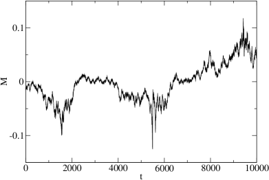
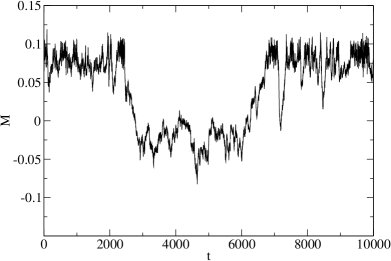
Figure 1 shows the magnetization $M(t)$ as a function of time ( sweep ). Following [31] we define the return $r(t)$ through the magnetization as

$$r(t)=M(t+1)-M(t),$$ (18)

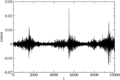
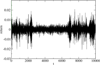
where $M(t)$ is the magnetization given by (4). Figure 2 shows time series of return $r(t)$ where we observe the intermittency of returns. As mentioned in section 2 such intermittent behavior is expected to be caused by the phase change. Namely the ordered phase where $|M|$ and its fluctuation are small corresponds to low-volatility phase. Conversely the disordered phase corresponds to high-volatility phase. These properties can also be confirmed by comparing figures 1 and 2. Since values of volatility are not obtained directly from returns we estimate them by the GARCH model as used in the volatility estimation in empirical finance.

Figure 3: Volatility time series obtained by the GARCH model: $\gamma=1.0$ (left) and $\gamma=0.05$ (right).

Figure 4: Return distribution (left) and standardized return distribution (right) simulated at $\gamma=1.0$. The red line shows the standard normal distribution.

Figure 5: Return distribution (left) and standardized return distribution (right) simulated at $\gamma=0.05$. The red line shows the standard normal distribution.

5 Volatility from the GARCH model

We apply the GARCH model for return data obtained from the financial spin model and estimate volatility corresponding to each return. The Bayesian inference of the GARCH model is performed by the Metropolis-Hastings algorithm with an adaptive multi-dimensional student’s t-distributions[37, 38, 39, 40]. In total we make $4\times 10^{4}$ Monte Carlo updates of GARCH parameters. The first $1.1\times 10^{4}$ updates are discarded as thermalization and the $2.9\times 10^{4}$ updates are used for analysis. At each update we also store the values of volatility and at the end we average the values of volatility for final output. The GARCH parameters determined by the Bayesian inference are listed in table 1. For both simulation parameters, values of $\alpha+\beta$ are found to be very close to 1, which means that the return time series obtained from those simulations have the strong persistency in volatility.

Table 1: Results of GARCH parameters. SD and SE stand for standard deviation and statistical error respectively. Statistical errors are estimated by the jackknife method. $\tau_{int}$ is the autocorrelation time defined by $\tau_{int}=1+2\sum_{i=1}^{\infty}ACF(t)$ where $ACF(t)$ stands for the autocorrelation function.

	$\alpha$	$\beta$	$\omega$
$\gamma=1.0$	0.0495	0.9508	$2.1\times 10^{-9}$
SD	0.0037	0.0013	$6\times 10^{-10}$
SE	0.00003	0.00003	$4\times 10^{-12}$
$\tau_{int}$	$1.8\pm 0.4$	$1.8\pm 0.3$	$1.8\pm 0.4$
$\gamma=0.05$	0.0836	0.9100	$8.6\times 10^{-8}$
SD	0.0055	0.0057	$1.4\times 10^{-8}$
SE	0.00003	0.00003	$8\times 10^{-11}$
$\tau_{int}$	$1.41\pm 0.05$	$1.40\pm 0.04$	$1.42\pm 0.05$

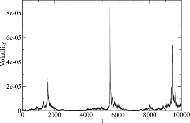
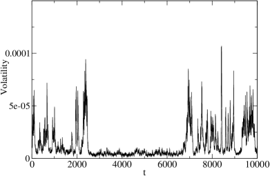
Figure 3 shows the time series of volatility obtained by the GARCH model. It is seen that there exist high-volatility and low-volatility periods. Such behavior of the volatility corresponds to ”volatility clustering” which often observed in the real financial markets.

Next we examine the view of the MDH for the return data from the financial spin model. In the MDH the return $r(t)$ is assumed to be given by $r(t)=\sigma_{t}\epsilon_{t}$, where $\sigma_{t}^{2}$ is volatility and $\epsilon_{t}$ is an independent Gaussian random variable with mean 0 and variance 1. Under this assumption the returns standardized by $\sigma_{t}$, i.e. $r(t)/\sigma_{t}$ should be standard normal random variables. Using volatility determined by the GARCH model as a proxy of the true volatility we standardize returns $r(t)$.

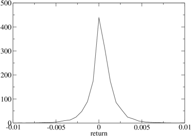
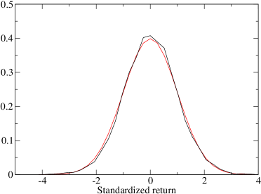
Figures 4 and 5 compare the distributions of the unstandardized and standardized returns. The unstandardized return distributions are very different from the standard normal distributions ( variance 1 and mean 0 ). On the other hand the standardized return distributions come close to the standard normal distributions that are depicted in red. The normality of the standardized returns can be further confirmed by examining variance and kurtosis.

Table 2 lists variance and kurtosis of the unstandardized and standardized returns. The variance and kurtosis of the unstandardized returns differ from the values expected for standard normal random variables, i.e. variance = 1 and kurtosis = 3. On the other hand it is remarkable that the variances of standardized returns from both simulations at $\gamma=1.0$ and 0.05 are consistent with 1. The values of kurtosis for standardized returns also come close to 3 although their values are slightly higher than 3. This small disagreement might be understood by that the GARCH model we used here, i.e. the GARCH(1,1) model with normal errors, still does not capture completely the properties of the return data from the spin financial model. The similar disagreement has been observed in the real financial markets[6].

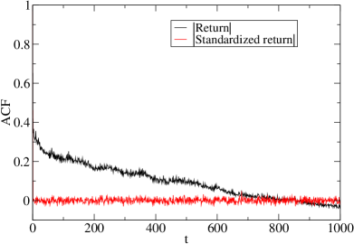
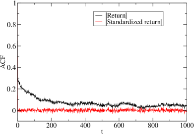
We further examine the MDH by calculating the autocorrelation function. As a stylized fact of asset returns it is known that the absolute return time series exhibits a very long correlation. However under the MDH the standardized returns are expected to be Gaussian random variables. Therefore if the MDH is hold we expect that the autocorrelation between the absolute standardized returns disappears. Figure 6 shows the autocorrelation functions of the absolute returns and absolute standardized returns. It is clear that the absolute returns show a very long correlation but the absolute standardized returns have no significant correlation. Thus this examination of the autocorrelation function also confirms the MDH for the return time series of the spin financial market. The similar behavior of the autocorrelation function on the absolute standardized returns is also observed in the real financial market[8].

Table 2: Variance and kurtosis of the unstandardized and standardized returns.

	$\gamma=1.0$		$\gamma=0.05$
	variance	kurtosis	variance	kurtosis
unstandardized	$2.7\times 10^{-6}\pm 9\times 10^{-7}$	$21\pm 9$	$1.3\times 10^{-5}\pm 2\times 10^{-6}$	$6.6\pm 0.8$
standardized	$0.997\pm 0.022$	$3.54\pm 0.09$	$0.999\pm 0.025$	$3.49\pm 0.10$

Figure 6: Autocorrelation functions of absolute returns and absolute standardized returns at $\gamma=1.0$ (left) and $\gamma=0.05$ (right).

6 Conclusions

The volatility of a financial spin model with three-states was investigated by the GARCH model. To determine volatility by the GARCH model the Bayesian inference by the MCMC method was applied. We find that volatility of the spin financial market exhibits ”volatility clustering” which is often observed in the real financial markets. In order to examine the MDH for the spin financial market we analyzed returns standardized by the volatility obtained from the GARCH model. Under the MDH the normality is expected for the standardized returns. We find that variance and kurtosis of the standardized returns are very similar to those of standard normal random variables except for a slightly higher kurtosis. The autocorrelations of the absolute standardized returns were also investigated and no significant autocorrelation between absolute standardized returns was found, which can also be expected from the MDH. From these findings it is concluded that the spin financial market we simulated here is consistent with the view of the MDH for the return dynamics.

References

- [1] Cont R 2001 Empirical Properties of Asset Returns: Stylized Facts and Statistical Issues Quantitative Finance 1 223–236
- [2] Clark P K 1973 A subordinated stochastic process model with finite variance for speculative prices Econometrica 41 135-155
- [3] Andersen T G, Bollerslev T, Diebold F X and Labys P 2000 Exchange Rate Returns Standardized by Realized Volatility are (Nealy) Gaussian Multinational Finance Journal 4 159–179
- [4] Andersen T G, Bollerslev T, Diebold F X and Ebens H 2001 The distribution of realized stock return volatility Journal of Financial Economics 61 43–76
- [5] Andersen T G, Bollerslev T and Dobrev, D 2007 No-arbitrage semi-martingale restrictions for continuous-time volatility models subject to leverage effects, jumps and i.i.d. noise: Theory and testable distributional implications Journal of Econometrics 138 125-180
- [6] Andersen T G, Bollerslev T, Frederiksen P and Nielsen M Ø 2010 Continuous-time models, realized volatilities, and testable distributional implications for daily stock returns Journal of Applied Econometrics 25 233-261
- [7] Fleming J and Paye B S 2011 High-frequency returns, jumps and the mixture of normals hypothesis Journal of Econometrics 160 119-128
- [8] Takaishi T, Chen TT and Zheng Z 2012 Analysis of Realized Volatility in Two Trading Sessions of the Japanese Stock Market Prog. Theor. Phys. Supplement 194 43-54
- [9] Takaishi T 2012 Finite-Sample Effects on the Standardized Returns of the Tokyo Stock Exchange Procedia - Social and Behavioral Sciences 65 968–973
- [10] Engle R F 1982 Autoregressive Conditional Heteroskedasticity with Estimates of the Variance of the United Kingdom inflation Econometrica 50 987–1007
- [11] Bollerslev T 1986 Generalized Autoregressive Conditional Heteroskedasticity Journal of Econometrics 31 307–327
- [12] Nelson D B 1991 Conditional Heteroskedasticity in Asset Returns: A New Approach Econometrica 59 347-370
- [13] Engle R F and Ng V 1993 Measuring and testing the impact of news on volatility Journal of Finance 48 1749-1778
- [14] Sentana E 1995 Quadratic ARCH models Review of Economic Studies 62 639-661
- [15] Glosten L R, Jaganathan R and Runkle D E 1993 On the Relation Between the Expected Value and the Volatility of the Nominal Excess on Stocks Journal of Finance 48 1779-1801
- [16] Ding Z, Granger C W J and Engle R F 1993 A long memory property of stock market returns and a new model Journal of Empirical Finance 1 83–106
- [17] Takaishi T and Chen TT 2012 Bayesian Inference of the GARCH model with Rational Errors International Proceedings of Economics Development and Research 29 303–307
- [18] Bollerslev T, Chou R Y and Kroner K F 1992 ARCH modeling in finance Journal of Econometrics 52 5–59
- [19] Cont R and Bouchaud J P 2000 Herd behaviour and aggregate fluctuations in financial markets Macroecon. Dynamics 4 170-196
- [20] Stauffer D and Penna T J P 1998 Crossover in the Cont-Bouchaud percolation model for market fluctuations Physica A 256 284–290
- [21] Sato A H and Takayasu H 1998 Dynamic numerical models of stock market price: from microscopic determinism ot macroscopic randomness Physica A 250 231–252
- [22] Lux T and Marchesi M 1999 Scaling and Criticality in a Stochastic Multi-Agent Model of a Financial Market Nature 397 498–500
- [23] Iori G 1999 Avalanche Dynamics and Trading Friction Effects on Stock Market Returns Int. J. Mod. Phys. C 10 1149–1162
- [24] da Silva L R and Stauffer D 2001 Ising-correlated clusters in the Cont-Bouchaud stock market model Physics A 294 235–238
- [25] Challet D, Marsili M and Zecchina R 2000 Statistical mechanics of system with heterogeneous agents: Minority games Phys. Rev. Lett. 84(8) 1824–1827
- [26] Raberto M, Cincotti S, Focardi S M and Marchesi M 2001 Agent-based Simulation of a Financial Market Physics A 299 319–327
- [27] Bornholdt S 2001 Expectation Bubbles in a Spin Model of Markets: Intermittency from Frustration across Scales Int. J. Mod. Phys. C 12 667–674
- [28] Sznajd-Weron K and Weron R 2002 A Simple Model of Price Formation Int. J. Mod. Phys. C 13 115–123
- [29] Sanchez J R 2002 A Simple Model for Stocks Markets Int. J. Mod. Phys. C 13 639–644
- [30] Yamano Y 2002 Bornholdt’s Spin Model of a Market Dynamics in High Dimensions Int. J. Mod. Phys. C 13 89–96
- [31] Kaizoji T, Bornholdt S and Fujiwara Y 2002 Dynamics of Price and Trading Volume in a Spin Model of Stock Markets with Heterogeneous Agents Physica A 316 441–452
- [32] Takaishi T 2005 Simulations of Financial Markets in a Potts-like Model Int. J. Mod. Phys. C 16 1311–1317
- [33] Krause S M and Bornholdt S 2011 Spin models as microfoundation of macroscopic financial market models arXiv:1103.5345
- [34] Stauffer D 2012 A Biased Review of Sociophysics J. Stat. Phys. 151 9–20
- [35] Matia K, Pal M, Salunkay H and Stanley H E 2004 Scale-dependent price fluctuations for the Indian stock market Europhys. Lett. 66 909–914
- [36] Akaike H 1973 Information theory and an extension of the maximum likelihood principle Proceedings of the 2nd International Symposium on Information Theory Petrov B N and Caski F (eds.), Akadimiai Kiado, Budapest: 267-281
- [37] Takaishi T 2009 An Adaptive Markov Chain Monte Carlo Method for GARCH Model Lecture Notes of the Institute for Computer Sciences, Social Informatics and Telecommunications Engineering. Complex Sciences Vol. 5 1424–1434
- [38] Takaishi T 2009 Bayesian Estimation of GARCH Model with an Adaptive Proposal Density New Advances in Intelligent Decision Technologies, Studies in Computational Intelligence Vol. 199 635–643
- [39] Takaishi T 2009 Bayesian Inference on QGARCH Model Using the Adaptive Construction Scheme Proceedings of 8th IEEE/ACIS International Conference on Computer and Information Science 525–529 doi:10.1109/ICIS.2009.173
- [40] Takaishi T 2010 Bayesian inference with an adaptive proposal density for GARCH models J. Phys.: Conf. Ser. 221 012011