Speeding up neighborhood search in
local Gaussian process prediction
Abstract
Recent implementations of local approximate Gaussian process models have pushed computational boundaries for non-linear, non-parametric prediction problems, particularly when deployed as emulators for computer experiments. Their flavor of spatially independent computation accommodates massive parallelization, meaning that they can handle designs two or more orders of magnitude larger than previously. However, accomplishing that feat can still require massive computational horsepower. Here we aim to ease that burden. We study how predictive variance is reduced as local designs are built up for prediction. We then observe how the exhaustive and discrete nature of an important search subroutine involved in building such local designs may be overly conservative. Rather, we suggest that searching the space radially, i.e., continuously along rays emanating from the predictive location of interest, is a far thriftier alternative. Our empirical work demonstrates that ray-based search yields predictors with accuracy comparable to exhaustive search, but in a fraction of the time—for many problems bringing a supercomputer implementation back onto the desktop.
Key words: approximate kriging, nonparametric regression, nearest neighbor, sequential design of experiments, active learning, big data
1 Introduction
Gaussian process (GP) regression is popular for response surface modeling wherever surfaces are reasonably smooth, but where otherwise little is known about the the input–output relationship. GP regression models are particularly popular as emulators for computer experiments (Sacks et al.,, 1989; Santner et al.,, 2003), whose outputs tend to exhibit both qualities. Moreover computer experiments are often deterministic, and it turns out that GPs are one of a few flexible regression approaches which can interpolate while also predicting accurately with appropriate coverage out-of-sample. Unfortunately GP regression requires dense matrix decompositions, for input–output pairs, so implementations struggle to keep up with today’s growing pace of data collection. Modern supercomputers make submitting thousands of jobs as easy as submitting one, and therefore runs is no longer a prototypically-sized computer experiment (Chen et al.,, 2013).
Most modern desktops cannot decompose dense matrices as large as , due primarily to memory constraints. They struggle to perform tens to hundreds of much smaller, decompositions required for numerical inference of unknown parameters, say by maximum likelihood, in reasonable time. Although humbly small by comparison to other literatures, like genetics or marketing, those limits define “big data” for computer experiments: the canonical models cannot cope with the modern scale of computer simulation.
A scramble is on for fast, approximate, alternatives (e.g., Kaufman et al.,, 2012; Sang and Huang,, 2012; Gramacy and Apley,, 2014), and a common theme is sparsity, leading to fast matrix decompositions. Some approaches increase data size capabilities by one-to-two orders of magnitude. Yet even those inroads are at capacity. Practitioners increasingly prefer much cruder alternatives, for example trees (Pratola et al.,, 2014; Gramacy et al.,, 2012; Chipman et al.,, 2012) which struggle to capture the smoothness of most simulators.
Another approach is to match supercomputer simulation with supercomputer emulation, e.g, using graphical processing units (GPUs, Franey et al.,, 2012), cluster, and symmetric-multiprocessor computation, and even all three together (Paciorek et al.,, 2013), for (dense matrix) GP regression. This too has led to orders of magnitude expansion in capability, but may miss the point: emulation is meant to avoid further computation. Hybrid approximate GP regression and big-computer resources have been combined to push the boundary even farther (Eidsvik et al.,, 2013). Gramacy et al., (2014b) later showed how GPUs and/or thousands of CPUs, distributed across a cluster, could be combined to handle designs as large as in about an hour.
This paper makes three contributions to this literature, focusing on a particular sparsity-inducing local GP approximation developed by Gramacy and Apley, (2014). First, we study a greedy search subroutine, applied locally and independently for each element of a potentially vast predictive grid. Each search identifies small local sub-designs by a variance reduction heuristic—the main sparsity-inducing mechanism—and we identify how it organically facilitates a desirable trade-off between local and (more) global site selection. We then observe highly regular patterns in the variance reduction surface searched in each iteration of the greedy scheme, motivating our second contribution. We propose swapping out an exhaustive discrete search for a continuous one having far narrower scope: along rays emanating from each predictive site. Our empirical work demonstrates that the new scheme yields accurate predictions in time comparable to a GPU/cluster computing implementation, yet only requires a modern desktop. Third, to acknowledge that rays can be inefficient in highly anisotropic contexts, we illustrate how a thrifty pre-scaling step from a crude global analysis leads to improved out-of-sample performance. Finally, the software modifications required are slight, and are provided in the updated laGP package for R (Gramacy,, 2013, 2014).
The remainder of the paper is outlined as follows. In Section 2 we survey the modern literature for fast approximate GP regression with an emphasis on sparsity and local search. Section 3 explores the structure of local designs, recommending the simple heuristic presented in Section 4. In Section 5 we provide implementation details and illustrations on real and simulated data from the recent literature. Section 6 concludes with a brief discussion.
2 Fast approximate Gaussian process regression
Here we review the basics of GP regression, emphasizing computational limitations and remedies separately leveraging sparsity and distributed computation. That sets the stage for a modern re-casting of a localization technique from the spatial statistics literature that is able to leverage both sparsity and big computing paradigms. Yet even that method has inefficiencies, which motivates our contribution.
2.1 Kriging and sparsity
A Gaussian process (GP) is a prior over functions (see, e.g., Stein,, 1999), with finite dimensional distributions defined parsimoniously by a mean and covariance, often paired with a error model (also Gaussian) for noisy data. However for regression applications, a likelihood perspective provides a more expedient view of the salient quantities. In a typical GP regression, data pairs , comprised of an -dimensional design and an -vector of scalar responses , is modeled as , where are a small number of parameters that relate the mean and covariance to covariates . Linear regression is a special case where and .
In the non-linear case it is typical, especially for computer experiments (e.g., Santner et al.,, 2003), to have a zero mean and therefore move all of the “modeling” into a correlation function so that where is a positive definite matrix comprised of pairwise evaluations on the rows of . Choice of determines the decay of spatial correlation throughout the input space, and thereby stationarity and smoothness. A common first choice is the so-called isotropic Gaussian: , where correlation decays very rapidly with lengthscale determined through . Since the resulting regression function is an interpolator, which is appropriate for many deterministic computer experiments. For noisy data, or for more robust modeling (protecting against numerical issues as well as inappropriate choice of covariance, e.g., assuming stationarity) of deterministic computer experiments (Gramacy and Lee,, 2012), a nugget can be added to . In this paper we will keep it simple and use the isotropic Gaussian formulation, and fix a small nugget for numerical stability. However, when appropriate we will explain why authors have made other choices, often for computational reasons. All new methodology described herein can be generalized to any correlation family that is differentiable in .
GP regression is popular because inference (for ) is easy, and (out-of-sample) prediction is highly accurate and conditionally (on ) analytic. It is common to deploy a reference prior (Berger et al.,, 2001) and obtain a marginal likelihood for
| (1) |
which has analytic derivatives, leading to fast Newton-like schemes for maximizing.
The predictive distribution , is Student- with degrees of freedom ,
| mean | (2) | ||||
| and scale | (3) |
where is the -vector whose component is . Using properties of the Student-, the variance of is . The form of , being small/zero for ’s in and expanding out in a “football shape” away from the elements of , has attractive uses in design: high variance inputs represent sensible choices for new simulations (Gramacy and Lee,, 2009).
The trouble with all this is and , appearing in several instances in Eqs. (1–3), and requiring computation for decomposing dense matrices. That limits data size to in reasonable time—less than one hour for inference and prediction on a commensurately sized -predictive-grid, say—without specialized hardware. Franey et al., (2012) show how graphical processing unit (GPU) matrix decompositions can accommodate in similar time. Paciorek et al., (2013) add an order of magnitude, to with a combination of cluster computing (with nearly 100 nodes, 16 cores each) and GPUs.
An alternative is to induce sparsity on and leverage fast sparse-matrix libraries, or to avoid large matrices all together. Kaufman et al., (2012) use a compactly supported correlation (CSC) function, , that controls the proportion of entries which are non-zero; Sang and Huang, (2012) provide a similar alternative. Snelson and Ghahramani, (2006) work with a smaller based on a reduced global design of pseudo-inputs, while Cressie and Johannesson, (2008) use a truncated basis expansion. Like the parallel computing options above, leveraging sparsity extends the dense-matrix alternatives by an order of magnitude. For example, Kaufman et al., (2012) illustrate with an cosmology dataset.
However, there is a need for bigger capability. For example, Pratola et al., (2014) choose a thrifty sum of trees model which allowed for cluster-style (message passing interface; MPI) implementation to perform inference for a 7-million sized design distributed over hundreds of computing cores. Until recently, such a large data set was well out of reach of GP based methods, whether by sparse approximation or distributed computation.
2.2 Local search
In computer experiments, where emulation or surrogate modeling emphasizes accurate prediction (2–3), Gramacy and Apley, (2014) showed how orders of magnitude faster inference and prediction can be obtained by modernizing local kriging from the spatial statistics literature (Cressie,, 1991, pp. 131–134). Focusing on quickly obtaining accurate predictive equations at a particular location, , local kriging involves choosing data subsets , based on whose values are close to . This recognizes that data far from have vanishingly small influence on prediction given the typical choices of rapidly decaying correlation functions . The simplest choice is to fill with nearest neighbors (NNs) to in , along with responses .
This is a sensible idea. As long as is determined purely by computational considerations, i.e., not by looking values, the result is a valid probability model for (Datta et al.,, 2014). For modest , prediction and inference is fast and accurate, and as gets large predictors increasingly resemble their full-data analogues with a variance that is organically inflated (higher variance for smaller ) relative to . Recently, Emory, (2009) showed that the NN version works well for a wide swath of common choices of . However, there is documented scope for improvement. Vecchia, (1988) and Stein et al., (2004) argue that the NN designs are sub-optimal—it pays to have a local design with more spread in the input space. However, finding an optimal local design , under almost any criteria, would involve a combinatorially huge search even for modest and .
Gramacy and Apley, (2014) showed how a greedy iterative search for local designs, starting with a small NN set and building up to by augmenting , for through a simple objective criteria leads to better predictions than NN. Importantly, the greedy and NN schemes can be shown to have the same computational order, , when an efficient updating scheme is deployed for each . The idea of building up designs iteratively for faster calculations is not new (Haaland and Qian,, 2011; Gramacy and Polson,, 2011), however the focus has previously been global. Gramacy and Apley,’s local search chooses an from the remaining set to maximally reduce predictive variance at . The local designs contain a mixture of NNs to and somewhat farther out “satellite” points, which we explore further in Section 3.
The resulting local predictors are at least as accurate as other sparse methods, like CSC, but incur an order of magnitude lower computational cost. Since calculations are independent for each predictive location, , prediction over a dense grid can be trivially parallelized to leverage multiple cores on a single (e.g., desktop) machine. However somewhat dissapointingly, Gramacy and Apley, also observed that the resulting greedy local predictors are not more accurate per-unit-computational cost than local NN predictors derived from an order of magnitude larger . In other words, the search for over a potentially huge number of candidates , for is expensive relative to decomposing a larger (but still small compared to ) matrix for GP inference and prediction.
Gramacy et al., (2014b) later recognized that that search, structured to independently entertain thousands of under identical criteria, is ideal for exporting to a GPU. Depending on the size of the search, improvements were 20–100 fold, leading to global improvements (over all ) of 5-20x, substantially out-pacing the accuracy-per-flop rate of a big-NN alternative. Going further, they showed how a GPU/multi-CPU/cluster scheme could combine to accurately emulate at one-million-sized designs in about an hour—a feat unmatched by other GP-based methodology.
Further savings are obtained by recognizing that searching over all candidates is overkill, whether via GPU or otherwise, since many are very far from and thus have almost no influence on prediction. Searching over NNs, say when -million yields substantial speedups, but multi-node/multi-core resources would still be required in large data contexts. Importantly, one must take care not to choose so small as to preclude entertaining the very points, well outside the NN set, which lead to improvements over NN. Considering the observed regularity of the greedy local designs, illustrated in more detail below, there does nevertheless seem to be potential for drastically shortcutting an exhaustive search without limiting scope, thereby avoiding the need for specialized (GPU) or cluster-computing resources.
3 Exploring local influence on prediction
The numbers in Figure 1 indicate local designs built up in a greedy fashion, successively choosing the next location by a reduction in variance criteria, discussed in detail shortly. Focus first on the black numbers, based on an exhaustive search. The reference predictive location, , is situated off of the input design , which is a regular grid in .
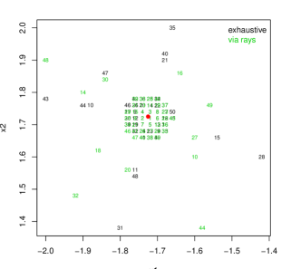
Observe that the local sub-design contains a roughly split comprising of the nearest elements in to and ones farther out. However even the farther-out elements are close relative to the full scope of the grid in . Observe that although many NNs are chosen in early iterations, the farthest-out locations are not exclusive to the final iterations of the search. As early as , a far-out excursion was made, and as late as a NN was chosen.
On first encounter, it may be surprising that having farther-out design elements helps reduce local predictive variance differentially more than points much closer in. One naturally wonders what trade-offs are being made in the objective criteria for design, and to what extent they can be attributed to a particular parameterization of . These two aspects are explored below, leading to novel technical and empirical observations, with an eye toward exploiting that trade-off for fast search in Section 4.
3.1 From global to local design
Designing to minimize predictive variance, averaged globally over the input space , is a sensible objective leading to so-called -optimal designs (see, e.g., Santner et al.,, 2003). However, minimizing over free coordinates in -dimensional space is combinatorially complex. Seo et al., (2000) showed that approximately -optimal designs can be obtained by proceeding sequentially, i.e., greedily: building up through choices of to augment to minimize variance globally. In particular, they considered choosing to minimize
where is the new variance after is added into , obtained by applying the predictive equations (2–3) with a -sized design . All quantities above, and below, depend implicitly on . Now, minimizing future variance is equivalent to maximizing a quantity proportional to a reduction in variance:
| (4) |
The designs that result are difficult to distinguish from other space-filling designs like maximin, maximum entropy, - or -optimal. The advantage is that greedy selection avoids a combinatorially huge search.
Gramacy and Apley, (2014) argued that the integrand in (4) is a sensible heuristic for local design. It tabulates a quantity proportional to reduction in variance at , obtained by choosing to add into the design, which is the dominating component in an estimate of the future mean-squared prediction error (MSPE) at that location. When applied sequentially to build up via and for , the result is again an approximate a solution to a combinatorially huge search. However, the structure of the resulting local designs , with near as well as far points, is counterintuitive [see Figure 1]. The typical rapidly decaying should substantially devalue locations far from . Therefore, considering two potential locations, an close to and farther away, one wonders: how could the latter choice, with -value modeled as vastly less correlated with than via , be preferred over the closer choice?
The answer is remarkably simple, and has little to do with the form of . The integrand in Eq. (4) looks quadratic in , the only part of the expression which measures a “distance”, in terms of correlation , between the reference predictive location and the potential new local design location . That would seem to suggest maximizing the criteria involves maximizing , i.e., choosing as close as possible to . But that’s not the only part of the expression which involves . Observe that the integrand is also quadratic in , a vector measuring “inverse distance”, via , between and the current local design . So there are two competing aims in the criteria: minimize “distance” to while maximizing “distance” (or minimizing “inverse distance”) from the existing design. Upon further reflection, that tradeoff makes sense. The value of a potential new data element depends not just on its proximity to , but also on how potentially different that information is from where we already have (lots of) it, at .
This observation also provides insight into the nature of global -optimal designs. We now recognize that the integral in Eq. (4), often thought to be essential to obtain space-filling behavior in the resulting design, is but one contributing aspect. Assuming that potential design sites for or are limited, say to a pre-defined mesh of values,111Note that this is always the case when working with a finite precision computer implementation. and that it is not possible to observe the true output at locations where you are trying to predict,222That would cause the integrand in (4) to be minimized trivially, and obliterate the need for emulation. the GP predictor prefers design sites which are somewhat spread out relative to where it will be used to predict, globally or locally, regardless of the choice of .
3.2 Ribbons and rings
Having established it is possible for the criteria to prefer new farther from , being repelled by already nearby, it is natural to wonder about the extent of that trade-off in particular examples: of iteration , choice of parameters (), and operational considerations such as how searches are initialized (a number of NNs) and any numerical considerations (i.e., nugget ). Here we restrict to the grid coinciding with the example in the previous subsection.
| , , | , , | , , | , , |
|---|---|---|---|
 |
 |
 |
 |
 |
 |
 |
 |
 |
 |
 |
 |
 |
 |
 |
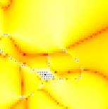 |
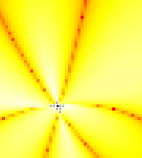
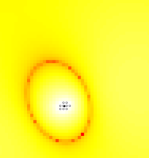
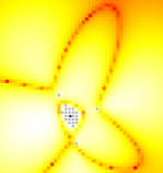
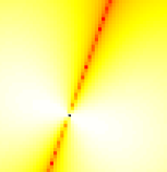
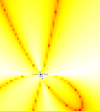
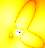
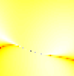
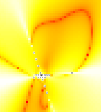
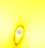
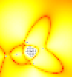
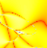
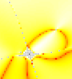
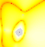
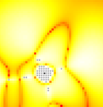
Figure 2 shows snapshots along the trajectory of four separate greedy searches (one in each column) for prediction at the same location, shown as a solid dot. The image plots show the reduction in variance criteria [integrand of (4)], with lighter shades being higher values, and open circles representing the current local design . The full set of plots for each of greedy selections are provided as supplementary material.
First some high level observations. The red ribbons and rings, carving out troughs of undesirable locations for future sampling, are fascinating. They persist, with some refinement, as greedy selections progress (down the rows), choosing elements of , the open circles. Moreover these selections, whether near to or far, impact future choices spanning great distances in both space and time, i.e., impacting many iterations into the future.
Now some lower level observations along the columns. Focusing on the first one, notice how the local design initially spans out in four rays emanating from . But eventually points off those rays are chosen, possibly forming new rays. The third column shows a similar progression, although the larger combined with smaller leads to a bigger proportion of NNs. The first and second rows in those columns show successive designs for and (however with different ), and it is interesting to see how those choices impact the resulting reduction in variance surface. In the first column, the choices “tie” a ribbon of red closer to in one corner of the design space. In the third, where the same behavior might be expected, instead the surface flattens out and a red ring is created around the new point.
The second and fourth column show more extreme behavior. In the second the large and lead to many NNs being chosen. However, eventually the design does fan out along rays, mimicking the behavior of the first and third columns. The fourth column stands out as exceptional. That search is initialized at and uses a nearly-zero nugget . The first dozen or so locations follow an arc emanating from , shown in the first two rows. Eventually, in the third row, the arc circles around on itself, creating a ring of points. However now some points off of the ring have also been selected, both near and far. The final row shows the ring converting into a spiral. More importantly, it shows a local design starting to resemble those from the other columns: NNs with satellite points positioned (loosely) along rays.
Our takeaway from this empirical analysis is that the pattern of local designs is robust to the choice of correlation parameters, although the proportion of NNs to satellite points, and the number of rays and their orientation is sensitive to those choices. We worked with a gridded design, which lent a degree of regularity to the illustration. In other experiments (not shown) we saw similar behavior as long as was space-filling. However, obviously if does not accommodate selecting local designs along rays, then an could not exhibit them. Below we suggest a searching strategy leveraging the patterns observed here, but which does not preclude discovering different local structure in a less idealized setting.
4 Exploiting local influence for efficient search
Here we exploit the partition between NNs and satellite points placed along rays observed in Section 3.2. We replace an exhaustive search amongst candidates with a continuous line search that can be solved quickly via a standard 1-d numerical optimizer, and then “snap” the solution back to the nearest element of the candidate set. Recognizing that the greedy local design pattern is sensitive to initialization and parameterization, as exemplified in Figure 2, our scheme is conservative about choosing search directions: looking along rays but not emphasizing the extension of existing ones.
Consider an existing local design and a search for along rays emanating from .
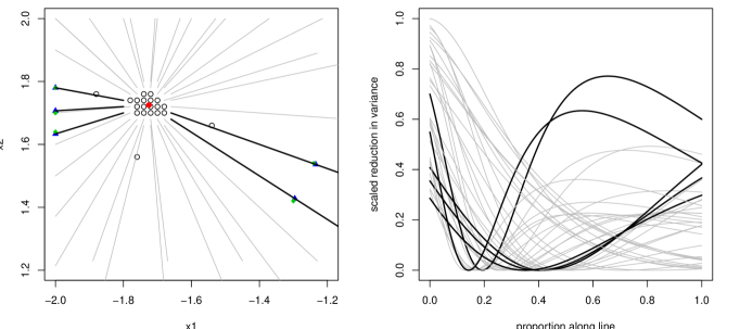
For example, the left panel of Figure 3 shows rays at iteration . Determining the start and end of the rays—i.e., the actual line segments—is discussed shortly. For each ray the corresponding 1-d graph of reduction in variance along the segment is shown in the right panel. Of the thirty five rays, five have a reduction in variance which is maximized away from its origin, at , and therefore away from the NN set. Those are shown in black, with blue triangles denoting the optima, and green diamonds indicating the closest element of the candidate set, , to that point. The right panel shows that if a random ray were chosen, the chances would be that a non NN point would be selected. For reference we note that the next satellite point is chosen by exhaustive search at .
We select the nearest candidates in to as potential starting points for a ray shooting in the opposite direction. There is no need to search between those nearest candidates and since there are, by definition, no remaining candidates there. We allow the segment to stretch to ten times the distance between the starting point and , or to the edge of the bounding box of the full candidate set . The rays in Figure 3 follow this rule. This choice allows the segments to grow in length as NNs accumulate in ; both the starts and ends of rays will be spaced farther from each other and from as increases. Although we show many rays in the figure, only a select few are considered in each iteration . These are based on a pseudo-random sequence on the NN candidates, following
Then, if the dimension of the input space is , we take closest elements to in as starting points for ray searches. The start of the sequence, , is designed to be a round robin over the nearest elements, where the scope of the “round” increases as increases, discouraging successive searches from identical starting points. Creating rays acknowledges that as the input dimension grows so too does the complexity of search, however number of rays could be a user-defined choice adjusting the speed (fewer rays is faster) and fidelity (but also cruder) as the situation recommends. We note that ray starting points could also be chosen randomly, however that would result in a stochastic local design , and therefore stochastic predictions, which would be undesirable in many contexts.
Any 1-d optimization scheme can be used to search over the convex combination
parameter , spanning the endpoints of the line segment. We use
the derivative-free Brent_fmin method
(Brent,, 1973), which is the workhorse behind R’s optimize
function, leveraging a C implementation of Fortran library
routines (http://www.netlib.org/fmm/fmin.f). A bespoke derivative-based
method could speed convergence, however we prefer the well-engineered library
routine in our setting of repeated application over for each of a potentially huge set of ’s. We recognize that
Brent_fmin’s’ initialization biases the solver towards solutions in
the interior of the search space, while we observe [see, e.g., Figures
2–3] that there is nearly always a mode at
the NN (), in addition to possibly multiple others. Therefore we check
against the mode as a post-processing step.
Optimizing over rays replaces an exhaustive discrete search with a continuous one,
providing a solution off the candidate set. So the final step
involves “snapping” onto , by
minimizing Euclidean distance. When performing that search, we explicitly
forbid the ray starting location(s) from being chosen, unless its location
agrees precisely with , i.e., unless Brent_fmin returns
. This prevents choosing a NN location known not to maximize the
search objective criteria.
Besides these modifications—pseudo random round-robin ray choice, numerical optimization over a convex combination, and snapping back to the candidate set—the proposed scheme is identical to the one described in Section 2.2. The green choices shown in Figure 1 show that the local designs based on ray search are qualitatively similar to the exhaustive ones. What remains is to demonstrate comparable out of sample predictive performance at substantially reduced computational cost.
5 Implementation and empirical comparison
The methodological developments described above, and all local GP comparators, are implemented in the laGP package on CRAN. The code is primarily in C and utilizes OpenMP for multi-core parallelization, as described by Gramacy and Apley, (2014). Our experiments distribute the local design over eight threads on a four-core hyperthreaded 2010-model iMac. GPU subroutines for parallelized exhaustive search of the reduction in variance criteria are also provided in the package, however we do not include any new runs leveraging that feature in the empirical work reported here. We will, however, compare to the timings on GPUs and multi-node implementations described by Gramacy et al., (2014b).
All local designs are coupled with local inference for the lengthscale, , via Newton-like maximization of the local posterior probabilities. We also consider second stage re-designs where sub-designs were re-calculated based on the local parameter estimates obtained from the first sub-designs, i.e., computing after . NN comparators do not benefit from a second-stage re-design, since the NN set is independent of . All exhaustive search variations use a limited set of NN candidates for each of size in order to keep computational costs manageable for those comparators. We primarily use , however there are some exceptions to match experiments reported in earlier work. No such limits are placed on ray based searches, however snapping to the nearest element of the candidate set could be sped up slightly with similarly narrowed search scope. Unless an exception is noted, each ray-based search in our experiments uses rays for -dimensional , however in the software this is a knob that can be adjusted by the user.
5.1 A synthetic 2-d data set
Consider a synthetic 2-d dataset, whose gridded input design in was used for illustrations earlier in the paper. The response follows , where .
| iMac | ||||||
|---|---|---|---|---|---|---|
| meth | stage | secs | RMSE | SD | 95%c | |
| ray | 200 | 2 | 2948.9 | 0.0002 | 0.0048 | 1.00 |
| ray | 200 | 1 | 1695.4 | 0.0004 | 0.0047 | 1.00 |
| ray | 50 | 2 | 87.8 | 0.0008 | 0.0061 | 1.00 |
| ext | 50 | 2 | 436.8 | 0.0008 | 0.0058 | 1.00 |
| ray | 50 | 1 | 45.6 | 0.0009 | 0.0061 | 1.00 |
| nn | 200 | 710.3 | 0.0010 | 0.0027 | 1.00 | |
| ext | 50 | 1 | 390.4 | 0.0010 | 0.0060 | 1.00 |
| nn | 50 | 11.5 | 0.0023 | 0.0045 | 1.00 | |
| sub | 1000 | 50.7 | 0.0369 | 0.0398 | 0.94 | |
| seconds | |||
|---|---|---|---|
| ext | rays | ||
| C/GPU | iMac | ||
| 50 | 1000 | 91 | 46 |
| 50 | 2000 | 120 | 46 |
| 128 | 2000 | 590 | 377 |
Table 1, left, summarizes a predictive experiment involving a grid of locations spaced to avoid . Since is extremely dense in the 2-d space, we opted for just one ray (rather than ) at each local design search. Using two rays gives slight improvements on RMSE, but requires nearly twice the computation time for the larger experiments. A more in-depth study of how the number of rays is related to accuracy is deferred to Section 5.4. The most important result from the table is that the ray-based method requires about 10–20% of the time compared to the exhaustive (“ext”) search, and performs at least as well by RMSE. Design by rays is also more accurate, and 10x faster than, a large NN comparator. The simple option of randomly sub-sampling a design of size 1000 (“sub”), and then performing inference and prediction under an isotropic model, requires commensurate computing resources but leads to poor accuracy results.333Estimating a separable global model on a subset of the data leads to similar accuracy/coverage results, since the data-generating mechanism has a high degree of radial symmetry, at greater computational expense required to numerically optimize over a vectorized parameter. Choosing the subset randomly also adds variability: a 95% interval for RMSE over thirty repeats is (0.0007, 0.0416). Space-filling sub-designs can substantially reduce that variability but at potentially great computational cost. For example, calculating an 1000-sized maximum entropy sub-design would cause compute times to go up by at least two orders of magnitude (with no change in mean performance) due to the multitude of calculations that would require.
Some other observations from the left-hand table include that a second stage design consistently improves accuracy, and that a large () search, which would require unreasonable computation (without a GPU) if exhaustive, is feasible via rays and leads to the best overall predictors. Although some methods report lower predictive SD than others, note that local approximations yield perfect coverage, which is typical with deterministic computer experiment data. The “sub” comparator achieves coverage close to the nominal 95% rate, but that ought not impress considering its poor RMSE results. Achieving nominal coverage is easy at the expense of accuracy, e.g., via constant and under a global Gaussian model. Achieving a high degree of accuracy at the expense of over-covering, and hence obtaining a conservative estimate of uncertainty, is a sensible tradeoff in our context.
Gramacy et al., (2014b) reported relative speedup times for a variant on the above experiment utilizing dual-socket 8-core 2.6 GHz 2013-model Intel Sandy Bridge compute cores, and up to two connected Nvidia Tesla M2090 GPU devices which massively parallelized the exhaustive search subroutine. The best times from those experiments, involving sixteen threads and both GPUs and one-stage design, are quoted on the right in Table 1. The accuracy of the predictions follow trends from the left table, however the timing information reveals that searching via rays is competitive with the exhaustive search even when that search subroutine is offloaded to a GPU. As the problem gets bigger (), the GPU exhaustive search and CPU ray-based search are competitive, but the ray method does not require limiting search to the nearby locations.
5.2 Langley Glide-back booster
Gramacy et al., presented timing results for emulation of a computer experiment simulating the lift of a rocket booster as it re-enters the atmosphere after disengaging from its payload. The design involved 37908 3-dimensional input settings and a predictive grid of size 644436. To demonstrate the supercomputing capability of local GPs on a problem of this size, they deploy exhaustive local search distributed over four identical 16-CPU-core/2-GPU nodes via the parallel library (in addition to OpenMP/CUDA) in R. Timings are presented for several different fidelities of local approximation. These numbers are shown in Table 2 alongside some new numbers of our own from a ray-based search on the iMac.
| minutes | |||||
|---|---|---|---|---|---|
| exhaust | rays | ||||
| 1x(16-CPU) | 4x(16-CPU) | 4x(16-CPU/2-GPU) | iMac | ||
| 50 | 1000 | 235 | 58 | 21 | 65 |
| 50 | 2000 | 458 | 115 | 33 | 65 |
| 50 | 10000 | 1895 | 476 | 112 | 65 |
| 128 | 2000 | - | 1832 | 190 | 1201 |
Observe that times for ray search on the iMac are in the ballpark of the exhaustive searches. Depending on and one style of search may be faster than another, however the exhaustive search clearly demands substantially more in the way of compute cycles. This a real-data experiment involved a large OOS predictive set for which no true-values of the output are known, so we were unable to explore how accuracy increases with fidelity.
5.3 The borehole data
The borehole experiment (Worley,, 1987; Morris et al.,, 1993) involves an 8-dimensional input space, and our use of it here follows the setup of Kaufman et al., (2012); more details can be found therein. We perform two similar experiments. In the first one, summarized in Table 3, we duplicate the experiment of Gramacy et al., (2014b) and perform out-of-sample prediction based on designs of increasing size . The designs and predictive sets (also of size ) are from a joint random Latin hypercube sample. As is increased so is the local design size so that there is steady reduction of out-of-sample MSE down the rows of the table. Gramacy et al., also increase , the size of the local candidate set, with , however the ray searches are not limited in this way.
| exhaustive | via rays | |||||||||
| Intel Sandy Bridge/Nvidia Tesla | iMac | Intel SB | ||||||||
| 96x CPU | 5x 2 GPUs | 1x(4-core) CPU | 96x CPU | |||||||
| seconds | mse | seconds | mse | seconds | mse | seconds | mse | |||
| 1000 | 40 | 100 | 0.48 | 4.88 | 1.95 | 4.63 | 8.00 | 6.30 | 0.39 | 6.38 |
| 2000 | 42 | 150 | 0.66 | 3.67 | 2.96 | 3.93 | 17.83 | 4.47 | 0.46 | 4.10 |
| 4000 | 44 | 225 | 0.87 | 2.35 | 5.99 | 2.31 | 40.60 | 3.49 | 0.62 | 2.72 |
| 8000 | 46 | 338 | 1.82 | 1.73 | 13.09 | 1.74 | 96.86 | 2.24 | 1.31 | 1.94 |
| 16000 | 48 | 507 | 4.01 | 1.25 | 29.48 | 1.28 | 222.41 | 1.58 | 2.30 | 1.38 |
| 32000 | 50 | 760 | 10.02 | 1.01 | 67.08 | 1.00 | 490.94 | 1.14 | 4.65 | 1.01 |
| 64000 | 52 | 1140 | 28.17 | 0.78 | 164.27 | 0.76 | 1076.22 | 0.85 | 9.91 | 0.73 |
| 128000 | 54 | 1710 | 84.00 | 0.60 | 443.70 | 0.60 | 3017.76 | 0.62 | 17.99 | 0.55 |
| 256000 | 56 | 2565 | 261.90 | 0.46 | 1254.63 | 0.46 | 5430.66 | 0.47 | 40.16 | 0.43 |
| 512000 | 58 | 3848 | 836.00 | 0.35 | 4015.12 | 0.36 | 12931.86 | 0.35 | 80.93 | 0.33 |
| 1024000 | 60 | 5772 | 2789.81 | 0.26 | 13694.48 | 0.27 | 32866.95 | 0.27 | 188.88 | 0.26 |
| 2048000 | 62 | - | - | - | - | - | - | - | 466.40 | 0.21 |
| 4096000 | 64 | - | - | - | - | - | - | - | 1215.31 | 0.19 |
| 8192000 | 66 | - | - | - | - | - | - | - | 4397.26 | 0.17 |
First focus on the timing and accuracy (MSE) results in the “iMac via rays” columns. The four columns to the left summarize the earlier experiment(s). By comparing the time column we see that the 4-core hyperthreaded iMac/rays implementation is about 2.5x times slower than the combined effort of 80 cores and 2 GPUs, or about 11.5x times slower than using more than 1500 cores. The amount of computing time for the largest run, at nine hours for more than one-million predictions on a one-million-sized design, is quite impressive for a nearly five-year-old desktop, compared to modern supercomputers (in earlier columns). However, looking at the accuracy column(s), we see that while the ray-based search is giving nearly identical results for the largest emulations, it is less accurate for the smaller ones. We attribute this to the size of the input space relative to the density of the smaller design(s), with two implications: (1) when designs are small, searching exhaustively is cheap, so a larger candidate set () relative to design size () can be entertained; (2) at the same time, since the design is sparse in high dimension when is small, the rays intersect fewer candidates, reducing the chances that the is close to the solution found along ray(s). In a large- small- setup, it may be best to search exhaustively.
The final pair of columns in Table 3 show timings and accuracies for runs with rays distributed over 96 Intel/Sandy Bridge 16-core machines. Observe how the running times are comparable to the exhaustive version, shown in column, until the pair . Neither method is fully utilizing the massively parallel potential of this supercomputer on “smaller” data. The exhaustive method is more accurate, if just slightly slower up until this point, so perhaps that method may be preferred in the “smaller” (but still huge for GPs) setting. But then the timings diverge, with rays showing big efficiency gains and nearly identical accuracy. By rays emulate more than twenty times faster. We then allowed rays to explore larger problems, to see what size data could be emulated in about an hour, ultimately finding that we can accommodate an 8x larger experiment while allowing the approximation fidelity to rise commensurately up to . This computational feat is unmatched in the computer modeling literature, whether via GPs or otherwise.
| subset iso | subset sep | rays with pre-scaled inputs | |||||||
|---|---|---|---|---|---|---|---|---|---|
| iMac | iMac | Intel SB | |||||||
| 1x(4-core) CPU, | 1x(4-core) CPU | 96x CPU | |||||||
| seconds | mse | seconds | mse | seconds | mse | seconds | mse | ||
| 1000 | 55.97 | 0.66 | 296.95 | 0.20 | 40 | 8.50 | 0.94 | 0.35 | 0.79 |
| 2000 | 55.82 | 0.38 | 220.62 | 0.11 | 42 | 19.73 | 0.38 | 0.50 | 0.47 |
| 4000 | 59.96 | 0.56 | 264.98 | 0.17 | 44 | 45.51 | 0.34 | 0.75 | 0.29 |
| 8000 | 60.04 | 0.50 | 288.19 | 0.11 | 46 | 111.14 | 0.22 | 1.46 | 0.23 |
| 16000 | 70.76 | 0.53 | 225.68 | 0.17 | 48 | 241.08 | 0.20 | 2.63 | 0.19 |
| 32000 | 89.75 | 0.50 | 362.09 | 0.13 | 50 | 547.10 | 0.16 | 4.86 | 0.15 |
| 64000 | 130.08 | 0.49 | 383.42 | 0.12 | 52 | 1208.15 | 0.13 | 9.13 | 0.13 |
| 128000 | 211.07 | 0.45 | 478.19 | 0.12 | 54 | 2732.71 | 0.11 | 19.50 | 0.12 |
| 256000 | 375.29 | 0.43 | 660.55 | 0.12 | 56 | 6235.47 | 0.11 | 41.80 | 0.11 |
| 512000 | 719.33 | 0.47 | 977.08 | 0.12 | 58 | 15474.62 | 0.10 | 82.56 | 0.10 |
| 1024000 | 1475.42 | 0.55 | 1690.75 | 0.13 | 60 | 38640.03 | 0.10 | 192.51 | 0.10 |
| 2048000 | - | - | - | - | 62 | - | - | 488.15 | 0.11 |
| 4096000 | - | - | - | - | 64 | - | - | 1234.56 | 0.11 |
| 8192000 | - | - | - | - | 66 | - | - | 4200.07 | 0.11 |
We are grateful to a referee for pointing out the importance comparing the results in Table 3 to a global GP predictor applied to a subset of the training data. In response we created Table 4 where columns 2–5 contain timings and MSE calculations obtained with random sub-designs under (estimated) isotropic and separable correlation functions. Note that although this part of the table is organized in rows for varying , the results here are (in expectation) independent of .444MSE variance decreases slightly down the rows as the testing set is increasing in size with . The borehole function is slowly varying across the input space, and highly stationary, so it is perhaps not surprising that a global isotropic GP (columns 2–3) fit on a subset compares favorably to the local ray-based alternative until . The borehole function is not uniformly sensitive to its inputs, so a global isotropic model is a poor fit, see e.g., Gramacy, (2014). The next pair of columns (4–5) show improved results with a separable model, although again these are noisy along the rows.
The final pair of columns come from a hybrid separable global model and local approximate one, via rays. Gramacy et al., (2014a) observed substantial performance boosts from pre-scaling inputs by the square-root global lengthscales estimated from data subsets. Although the local nature of inference and prediction accommodates a limited degree of nonstationarity, and thus anisotropy, if the data is highly globally anisotropic (as is the case for the borehole example), pre-scaling offers several benefits. One is statistical efficiency: global trends are best estimated on global scales. Another is computational: rays search radially, and therefore best mimic exhaustive searches when patterns in the variance reduction surface are loosely isotropic (as in Figure 2). Pre-scaling aligns the two more closely in that respect; more detailes are provided by Gramacy, (2014). The final two columns (7–8) show this hybrid approach outperforming the rest from about . Progress appears to plateau past million, due partly to rounding error/statistical noise, and partly to growing too slowly relative to in this setup.
5.4 Predictive accuracy and computation time
The comparison above duplicated a simulation setup from earlier work that was carefully designed to illustrate performance under increasing fidelity of approximation as data sizes increase. Here we consider a direct pitting of accuracy versus compute time in several views. In addition to the borehole data we consider the so-called Zhou, (1998) simulation and the piston simulation function (Kenett,, 1998; Ben-Ari and Steinberg,, 2007). The Zhou function can be applied for a range of input dimensions. Our first experiment, below, follows An and Owen, (2001) in using dimensions. We use the log of the response as the data-generating process involves products of exponentials that cause modeling challenges (and numerical instability) for larger . The piston data is 7-dimensional. For more details on both benchmarks see the library compiled by Surjanovic and Bingham, (2014), an excellent resource for benchmark problems involving computer simulation and associated applications.


Figure 4 shows six boxplots, paired vertically, with a column for each of three simulation setups. The top row summarizes compute times in seconds and bottom one has RMSEs obtained over thirty repeated Monte Carlo test and training sets. The borehole experiment used LHS training sets with K, and the other two used K. All three involved LHS testing sets of size 10000. The local approximate GP method, via rays, used for the borehole data, and for the other two. Large choices of and for the borehole experiment, relative to the others, are motivated by the smoothness observed in the previous comparison. Comparisons are drawn to random-subsample GP predictors using an isotropic correlation (“sub”), a separable version (“sub-sep”), and a rays version applied after re-scaling the inputs based on (the square root of) those estimated lengthscales.
A result common to all three experiments, echoing earlier observations, is that the variability in sub-sampled GP estimators, both by time and by RMSE, is high. Given a particular random training design, it is hard to predict how many iterations, involving expensive matrix inverses, will be required to learn the lengthscale(s). The local approximation(s) perform best in four of the six comparisons being made to sub-sampled versions with the same correlation structure. Estimating a separable global lenghscale is clearly desirable, whether for local or global emulation, if global isotropy is a poor approximation. The Zhou (1998) data is highly isotropic, so only in that case are the isotropic methods best.


Figure 5 shows the outcome of variations on Zhou (1998) experiments as input dimensions range for and the number of rays used in local search vary from one to . The image plots report averages over thirty repeats with (besides the input dimension) the same setup as described above. Since the scale of the response changes as varies, the RMSEs reported in the left pane are normalized by the minimum value obtained across the thirty repetitions. Observe that, for a fixed number of rays, RMSE deterioriates as the dimension increases. Allowing the number of rays to match keeps them steady. The color legend indicates that the performance gain is never better than 10% on the normalized RMSE scale. Also, we remark that there is no gain to having even more than rays (not shown). The right pane shows compute time growing more quickly for the number of rays than for .
6 Discussion
Approximate Gaussian process (GP) prediction is becoming essential for emulating simulation experiment output of the size generated by modern supercomputers. In this paper we focused on a local approach to emulation, building up local sub-designs containing input locations nearby to where predictions are required. By empirically studying the topology of surfaces depicting potential for reduction in predictive variance, the main objective behind the local design scheme, we discovered a regularity that was not being exploited by an exhaustive search. Instead, we suggested a continuous 1-d line search along rays emanating from the predictive location of interest, mimicking patterns of local designs observed in practice. We then showed, empirically, how the resulting ray-based designs yielded comparable out-of-sample predictive performance in a fraction of the time.
We discussed how conclusions from the exploratory analysis in Section 3 were independent of the choice of correlation function , in part justifying our use of the simple isotropic Gaussian family for our empirical work. We remarked that that choice only constrains the process locally. Global predictive properties may still be non-isotropic, and even non-stationary if parameterization is allowed to vary over the input space; see Gramacy and Apley, (2014) for further discussion. When the response surfaces are highly anisotropic on a global scale, like with the borehole data, pre-scaling the inputs based on a crude global analysis can yield substantial improvements; further discussion is offered by Gramacy et al., (2014a) and in the laGP software vignette (Gramacy,, 2014). There are many other situations in which the data might be better modeled by richer families of , and these certainly would impact local designs. In our supplementary material we provide trajectories of local designs, like the ones in Figure 2, for several relevant choices. Qualitatively however, similarities outnumber differences. Ribbons and rings are still present in the reduction in variance surface, and the designs that result are still a mix of NNs and satellite points.
Qualifications may be required in the context of smoothing noisy data, whether from stochastic simulation experiments or from spatial/geostatistical data under measurement error. In that case the covariance structure must be augmented with a nugget, which in turn must be estimated. Even in the deterministic computer experiments context, authors have argued that estimating a nugget may lead to improved out-of-sample predictive performance (e.g., Gramacy and Lee,, 2012; Andrianakis and Challenor,, 2012). Neither case has yet been adequately explored in the local approximate GP context. Although Gramacy, (2014) provides an example where locally estimated nuggets accurately capture the heteroskedastic input–output relationship in a simple example, it is clear that without further regularization applied to the rate of change of variance (spatially), both mean and variance surfaces will appear unstable (spatially), especially win low signal-to-noise contexts and in higher dimension. In particular, predictive surfaces will lack a sufficient aesthetic smoothness so as to be visually “recognizable” as (approximate) GP predictors.
Finally, while searching with rays led to big speedups and accurate approximate emulation for large designs, such schemes are not always appropriate. We saw that when designs are small and the dimension large—meaning that the density of points in the space is low—searching exhaustively is likely to lead to better out-of-sample prediction and, in the supercomputing setup, better value for a computational budget. Increasing the number of rays may help improve on accuracy, although the extra computation may not be warranted in small-to-moderately sized emulation problems. We also remark here that another disadvantage, especially in the distributed supercomputing context, is that ray-based searches can have uncertain times to convergence. We have observed that the slowest searches can require twice the number of objective (reduction in variance) evaluations than the average over a large set of problems ranging over both and . The exhaustive search, by comparison, has a deterministic runtime assuming operating system “noise” is low. Random convergence times can present a load balancing challenge when trying to make the most out of a supercomputing resource. However, as the timings in Table 3 show, the ray-based searches are so fast for the largest problems that perhaps such a small inefficiency might go unnoticed.
Acknowledgments
This work was completed in part with resources provided by the University of Chicago Research Computing Center. We are grateful for the valuable comments of an anonymous referee, which led to substantial improvements in the revised draft.
References
- An and Owen, (2001) An, J. and Owen, A. (2001). “Quasi-regression.” Journal of Complexity, 17, 4, 588–607.
- Andrianakis and Challenor, (2012) Andrianakis, I. and Challenor, P. (2012). “The effect of the nugget on Gaussian process emulators of computer models.” Computational Statistics & Data Analysis, 56, 12, 4125–4228.
- Ben-Ari and Steinberg, (2007) Ben-Ari, E. and Steinberg, D. (2007). “Modeling Data from Computer Experiments: and empirical comparison of kriging with MARS and projection pursuit regression.” Quality Engineering, 19, 4, 327–338.
- Berger et al., (2001) Berger, J., De Oliveira, V., and Sanso, B. (2001). “Objective Bayesian Analysis of Spatially Correlated Data.” Journal of the American Statistical Association, 96, 1361–1374.
- Brent, (1973) Brent, R. (1973). Algorithm for Minimization without Derivatives. Englewood Cliffs, N.J.: Prentice–Hall.
- Chen et al., (2013) Chen, H., Loeppky, J., Sacks, J., and Welch, W. (2013). “Analysis Methods for Computer Experiments: How to Assess and What Counts?” Tech. rep., University of British Columbia.
- Chipman et al., (2012) Chipman, H., Ranjan, P., and Wang, W. (2012). “Sequential Design for Computer Experiments with a Flexible Bayesian Additive Model.” Canadian Journal of Statistics, 40, 4, 663–678.
- Cressie, (1991) Cressie, N. (1991). Statistics for Spatial Data, revised edition. John Wiley and Sons, Inc.
- Cressie and Johannesson, (2008) Cressie, N. and Johannesson, G. (2008). “Fixed Rank Kriging for Very Large Data Sets.” Journal of the Royal Statistical Soceity, Series B, 70, 1, 209–226.
- Datta et al., (2014) Datta, A., Banerjee, S., Finley, A. O., and Gelfand, A. E. (2014). “Hierarchical Nearest-Neighbor Gaussian Process Models for Large Geostatistical Datasets.” Tech. rep., Univeristy of Minnesota. ArXiv:1406.7343.
- Eidsvik et al., (2013) Eidsvik, J., Shaby, B. A., Reich, B. J., Wheeler, M., and Niemi, J. (2013). “Estimation and prediction in spatial models with block composite likelihoods.” Journal of Computational and Graphical Statistics, 0, Accepted for publication, –.
- Emory, (2009) Emory, X. (2009). “The kriging update equations and their application to the selection of neighboring data.” Computational Geosciences, 13, 3, 269–280.
- Franey et al., (2012) Franey, M., Ranjan, P., and Chipman, H. (2012). “A Short Note on Gaussian Process Modeling for Large Datasets using Graphics Processing Units.” Tech. rep., Acadia University.
- Gramacy, (2014) Gramacy, R. (2014). “laGP: Large-Scale Spatial Modeling via Local Approximate Gaussian Processes in R.” Tech. rep., The University of Chicago. Available as a vignette in the laGP package.
- Gramacy et al., (2014a) Gramacy, R., Bingham, D., Holloway, J. P., Grosskopf, M. J., Kuranz, C. C., Rutter, E., Trantham, M., and Drake, P. R. (2014a). “Calibrating a large computer experiment simulating radiative shock hydrodynamics.” Tech. rep., The University of Chicago. ArXiv:1410.3293.
- Gramacy and Lee, (2012) Gramacy, R. and Lee, H. (2012). “Cases for the nugget in modeling computer experiments.” Statistics and Computing, 22, 3.
- Gramacy et al., (2014b) Gramacy, R., Niemi, J., and Weiss, R. (2014b). “Massively Parallel Approximate Gaussian Process Regression.” Tech. rep., The University of Chicago. ArXiv:1310.5182.
- Gramacy and Polson, (2011) Gramacy, R. and Polson, N. (2011). “Particle Learning of Gaussian Process Models for Sequential Design and Optimization.” Journal of Computational and Graphical Statistics, 20, 1, 102–118.
- Gramacy, (2013) Gramacy, R. B. (2013). laGP: Local approximate Gaussian process regression. R package version 1.0.
- Gramacy and Apley, (2014) Gramacy, R. B. and Apley, D. W. (2014). “Local Gaussian process approximation for large computer experiments.” Journal of Computational and Graphical Statistics. to appear; see arXiv:1303.0383.
- Gramacy and Lee, (2009) Gramacy, R. B. and Lee, H. K. H. (2009). “Adaptive Design and Analysis of Supercomputer Experiments.” Technometrics, 51, 2, 130–145.
- Gramacy et al., (2012) Gramacy, R. B., Taddy, M. A., and Wild, S. (2012). “Variable Selection and Sensitivity Analysis via Dynamic Trees with an Application to Computer Code Performance Tuning.” Annals of Applied Statistics, 7, 1, 51–80. ArXiv: 1108.4739.
- Haaland and Qian, (2011) Haaland, B. and Qian, P. (2011). “Accurate Emulators for Large-Scale Computer Experiments.” Annals of Statistics, 39, 6, 2974–3002.
- Kaufman et al., (2012) Kaufman, C., Bingham, D., Habib, S., Heitmann, K., and Frieman, J. (2012). “Efficient Emulators of Computer Experiments Using Compactly Supported Correlation Functions, With An Application to Cosmology.” Annals of Applied Statistics, 5, 4, 2470–2492.
- Kenett, (1998) Kenett, R. anmd Zacks, S. (1998). Modern Industrial Statistics: design and control of quality and reliability. Pacific Grove, CA: Duxbury Press.
- Morris et al., (1993) Morris, D., Mitchell, T., and Ylvisaker, D. (1993). “Bayesian Design and Analysis of Computer Experiments: Use of Derivatives in Surface Prediction.” Technometrics, 35, 243–255.
- Paciorek et al., (2013) Paciorek, C., Lipshitz, B., Zhuo, W., Prabhat, Kaufman, C., and Thomas, R. (2013). “Parallelizing Gaussian Process Calculations in R.” Tech. rep., University of California, Berkeley. ArXiv:1303.0383.
- Pratola et al., (2014) Pratola, M. T., Chipman, H., Gattiker, J., Higdon, D., McCulloch, R., and Rust, W. (2014). “Parallel Bayesian Additive Regression Trees.” Journal of Computational and Graphical Statistics, 23, 3, 830–852.
- Sacks et al., (1989) Sacks, J., Welch, W. J., Mitchell, T. J., and Wynn, H. P. (1989). “Design and Analysis of Computer Experiments.” Statistical Science, 4, 409–435.
- Sang and Huang, (2012) Sang, H. and Huang, J. Z. (2012). “A Full Scale Approximation of Covariance Functions for Large Spatial Data Sets.” Journal of the Royal Statistical Society: Series B, 74, 1, 111–132.
- Santner et al., (2003) Santner, T. J., Williams, B. J., and Notz, W. I. (2003). The Design and Analysis of Computer Experiments. New York, NY: Springer-Verlag.
- Seo et al., (2000) Seo, S., Wallat, M., Graepel, T., and Obermayer, K. (2000). “Gaussian Process Regression: Active Data Selection and Test Point Rejection.” In Proceedings of the International Joint Conference on Neural Networks, vol. III, 241–246. IEEE.
- Snelson and Ghahramani, (2006) Snelson, E. and Ghahramani, Z. (2006). “Sparse Gaussian Processes using Pseudo-inputs.” In Advances in Neural Information Processing Systems, 1257–1264. MIT press.
- Stein, (1999) Stein, M. L. (1999). Interpolation of Spatial Data. New York, NY: Springer.
- Stein et al., (2004) Stein, M. L., Chi, Z., and Welty, L. J. (2004). “Approximating Likelihoods for Large Spatial Data Sets.” Journal of the Royal Statistical Society, Series B, 66, 2, 275–296.
- Surjanovic and Bingham, (2014) Surjanovic, S. and Bingham, D. (2014). “Virtual Library of Simulation Experiments: Test Functions and Datasets.” Retrieved December 4, 2014, from http://www.sfu.ca/~ssurjano.
- Vecchia, (1988) Vecchia, A. (1988). “Estimation and model identification for continuous spatial processes.” Journal of the Royal Statistical Soceity, Series B, 50, 297–312.
- Worley, (1987) Worley, B. (1987). “Deterministic Uncertainty Analysis.” Tech. Rep. ORN-0628, National Technical Information Service, 5285 Port Royal Road, Springfield, VA 22161, USA.
- Zhou, (1998) Zhou, Y. (1998). “Adaptive importance sampling for integration.” Ph.D. thesis.